Implicit Finite-Horizon Approximation and Efficient Optimal Algorithms for Stochastic Shortest Path

Abstract

We introduce a generic template for developing regret minimization algorithms in the Stochastic Shortest Path (SSP) model, which achieves minimax optimal regret as long as certain properties are ensured. The key of our analysis is a new technique called implicit finite-horizon approximation, which approximates the SSP model by a finite-horizon counterpart only in the analysis without explicit implementation. Using this template, we develop two new algorithms: the first one is model-free (the first in the literature to our knowledge) and minimax optimal under strictly positive costs; the second one is model-based and minimax optimal even with zero-cost state-action pairs, matching the best existing result from (Tarbouriech et al., 2021b). Importantly, both algorithms admit highly sparse updates, making them computationally more efficient than all existing algorithms. Moreover, both can be made completely parameter-free.

1 Introduction

We study the Stochastic Shortest Path (SSP) model, where an agent aims to reach a goal state with minimum cost in a stochastic environment. SSP is well-suited for modeling many real-world applications, such as robotic manipulation, car navigation, and others. Although it is widely studied empirically (e.g., (Andrychowicz et al., 2017; Nasiriany et al., 2019)) and in optimal control theory (e.g., (Bertsekas and Tsitsiklis, 1991; Bertsekas and Yu, 2013)), it has received less attention under the regret minimization setting where a learner needs to learn the environment and improve her policy on-the-fly through repeated interaction. Specifically, the problem proceeds in $K$ episodes. In each episode, the learner starts at a fixed initial state, sequentially takes action, suffers some cost, and transits to the next state, until reaching a predefined goal state. The performance of the learner is measured by her regret, which is the difference between her total costs and that of the best policy.

Tarbouriech et al. (2020a) develop the first regret minimization algorithm for SSP with a regret bound of $\tilde{\mathcal{O}}(D^{3/2}S\sqrt{AK/c_{\min}})$, where $D$ is the diameter, $S$ is the number of states, $A$ is the number of actions, and $c_{\min}$ is the minimum cost among all state-action pairs. Cohen et al. (2020) improve over their results and give a near optimal regret bound of $\tilde{\mathcal{O}}(B_{\star}S\sqrt{AK})$, where $B_{\star}\leq D$ is the largest expected cost of the optimal policy starting from any state. Even more recently, Cohen et al. (2021) achieve minimax regret of $\tilde{\mathcal{O}}(B_{\star}\sqrt{SAK})$ through a finite-horizon reduction technique, and concurrently Tarbouriech et al. (2021b) also propose minimax optimal and parameter-free algorithms. Notably, all existing algorithms are model-based with space complexity $\Omega(S^{2}A)$. Moreover, they all update the learner’s policy through full-planning (a term taken from (Efroni et al., 2019)), incurring a relatively high time complexity.

In this work, we further advance the state-of-the-art by proposing a generic template for regret minimization algorithms in SSP (Algorithm 1), which achieves minimax optimal regret as long as some properties are ensured. By instantiating our template differently, we make the following two key algorithmic contributions:

• In Section 4, we develop the first model-free SSP algorithm called LCB-Advantage-SSP (Algorithm 2). Similar to most model-free reinforcement learning algorithms, LCB-Advantage-SSP does not estimate the transition directly, enjoys a space complexity of $\tilde{\mathcal{O}}(SA)$, and also takes only $\mathcal{O}\left(1\right)$ time to update certain statistics in each step, making it a highly efficient algorithm. It achieves a regret bound of $\tilde{\mathcal{O}}(B_{\star}\sqrt{SAK}+B_{\star}^{5}S^{2}A/c_{\min}^{4})$, which is minimax optimal when $c_{\min}>0$. Moreover, it can be made parameter-free without worsening the regret bound.

• In Section 5, we develop another simple model-based algorithm called SVI-SSP (Algorithm 3), which achieves minimax regret $\tilde{\mathcal{O}}(B_{\star}\sqrt{SAK}+B_{\star}S^{2}A)$ even when $c_{\min}=0$, matching the best existing result by Tarbouriech et al. (2021b). Notably, compared to their algorithm (as well as other model-based algorithms), SVI-SSP is computationally much more efficient since it updates each state-action pair only logarithmically many times, and each update only performs one-step planning (again, a term taken from (Efroni et al., 2019)) as opposed to full-planning (such as value iteration or extended value iteration); see more concrete time complexity comparisons in Section 5. SVI-SSP can also be made parameter-free following the idea of (Tarbouriech et al., 2021b).

We include a summary of regret bounds of all existing SSP algorithms as well as more complexity comparisons in Appendix A.

Techniques

Our main technical contribution is a new analysis framework called implicit finite-horizon approximation (Section 3), which is the key to analyze algorithms developed from our template. The high level idea is to approximate an SSP instance by a finite-horizon counterpart. However, the approximation only happens in the analysis, a key difference compared to (Chen et al., 2021; Chen and Luo, 2021; Cohen et al., 2021) that explicitly implement such an approximation in their algorithms. As a result, our method not only avoids blowing up the space complexity by a factor of the horizon, but also allows one to derive a horizon-free regret bound (more explanation to follow).

In order to achieve the minimax optimal regret, our model-free algorithm LCB-Advantage-SSP uses a key variance reduction idea via a reference-advantage decomposition by (Zhang et al., 2020b). However, crucial distinctions exist. For example, we update the reference value function more frequently instead of only one time, which helps reduce the sample complexity and improve the lower-order term in the regret bound. We also maintain an empirical upper bound on the value function in a doubling manner, which is the key to eventually make the algorithm parameter-free. On the other hand, for our model-based algorithm SVI-SSP, we adopt a special Bernstein-style bonus term and bound the learner’s total variance via recursion, taking inspiration from (Tarbouriech et al., 2021b; Zhang et al., 2020a).

Empirical Evaluation

We support our theoretical findings with experiments in Appendix H. Our model-free algorithm demonstrates a better convergence rate compared to vanilla Q learning with naive $\epsilon$-greedy exploration. Our model-based algorithm has competitive performance compared to other model-based algorithms, while spending the least amount of time in updates.

Related Work

For a detailed comparison of existing results for the same problem, we refer the readers to (Tarbouriech et al., 2021b, Table 1) as well as our Table 1. There are also several works (Rosenberg and Mansour, 2020; Chen et al., 2021; Chen and Luo, 2021) that consider the even more challenging SSP setting where the cost function is decided by an adversary and can change over time. Apart from regret minimization, Tarbouriech et al. (2021a) study the sample complexity of SSP with a generative model; Lim and Auer (2012) and Tarbouriech et al. (2020b) investigate exploration problems involving multiple goal states (multi-goal SSP).

The special case of SSP with a fixed horizon has been studied extensively, for both stochastic costs (e.g., (Azar et al., 2017; Jin et al., 2018; Efroni et al., 2019; Zanette and Brunskill, 2019; Zhang et al., 2020a)) and adversarial costs (e.g., (Neu et al., 2012; Zimin and Neu, 2013; Rosenberg and Mansour, 2019; Jin et al., 2020)). Importantly, recent works (Wang et al., 2020; Zhang et al., 2020a) find that when the cost for each episode is at most a constant, it is in fact possible to obtain a regret bound with only logarithmic dependency on the horizon. Tarbouriech et al. (2021b) generalize this concept to SSP and define horizon-free regret as a bound with only logarithmic dependence on the expected hitting time of the optimal policy starting from any state (which is bounded by $B_{\star}/c_{\min}$). They also propose the first algorithm with horizon-free regret for SSP, which is important for arguing minimax optimality even when $c_{\min}=0$. Notably, our model-based algorithm SVI-SSP also achieves horizon-free regret (but the model-free one does not).

2 Preliminaries

An SSP instance is defined by a Markov Decision Process (MDP) $M=({\mathcal{S}},{\mathcal{A}},s_{\text{init}},g,c,P)$, where ${\mathcal{S}}$ is the state space, ${\mathcal{A}}$ is the action space, $s_{\text{init}}\in{\mathcal{S}}$ is the initial state, and $g\notin{\mathcal{S}}$ is the goal state. When taking action $a$ in state $s$, the learner suffers a cost drawn in an i.i.d manner from an unknown distribution with mean $c(s,a)\in[0,1]$ and support $[c_{\min},1]$ ($c_{\min}\geq 0$), and then transits to the next state $s^{\prime}\in{\mathcal{S}}^{+}={\mathcal{S}}\cup\{g\}$ with probability $P_{s,a}(s^{\prime})$. We assume that the transition $P$ and the cost mean $c$ are unknown to the learner, while all other parameters are known.

The learning process goes as follows: the learner interacts with the environment for $K$ episodes. In the $k$-th episode, the learner starts in initial state $s_{\text{init}}$, sequentially takes an action, suffers a cost, and transits to the next state until reaching the goal state $g$. More formally, at the $i$-th step of the $k$-th episode, the learner observes the current state $s^{k}_{i}$ (with $s^{k}_{1}=s_{\text{init}}$), takes action $a^{k}_{i}$, suffers a cost $c^{k}_{i}$, and transits to the next state $s^{k}_{i+1}\sim P_{s^{k}_{i},a^{k}_{i}}$. An episode ends when the current state is $g$, and we define the length of episode $k$ as $I_{k}$, such that $s^{k}_{I_{k}+1}=g$.

Learning Objective

At a high level, the learner’s goal is to reach the goal with a small total cost. To this end, we focus on proper policies — a (stationary and deterministic) policy $\pi:{\mathcal{S}}\rightarrow{\mathcal{A}}$ is a mapping that assigns an action $\pi(s)$ to each state $s\in{\mathcal{S}}$, and it is proper if the goal is reached with probability $1$ when following $\pi$ (that is, taking action $\pi(s)$ whenever in state $s$). Given a proper policy $\pi$, one can define the cost-to-go function $V^{\pi}:{\mathcal{S}}\rightarrow[0,\infty)$ as $V^{\pi}(s)=\mathbb{E}\left[\left.\sum_{i=1}^{I}c_{i}\right|P,\pi,s_{1}=s\right],$ where the expectation is with respect to the randomness of the cost $c_{i}$ incurred at state-action pair $(s_{i},\pi(s_{i}))$, next state $s_{i+1}\sim P_{s_{i},\pi(s_{i})}$, and the number of steps $I$ before reaching $g$. The optimal proper policy $\pi^{\star}$ is then defined as a policy such that $V^{\pi^{\star}}(s)=\min_{\pi\in\Pi}V^{\pi}(s)$ for all $s\in{\mathcal{S}}$, where $\Pi$ is the set of all proper policies assumed to be nonempty. The formal objective of the learner is then to minimize her regret against $\pi^{\star}$, the difference between her total cost and that of the optimal proper policy, defined as

$$R_{K}=\sum_{k=1}^{K}\sum_{i=1}^{I_{k}}c^{k}_{i}-K\cdot V^{\star}(s_{\text{init}}),$$

where we use $V^{\star}$ as a shorthand for $V^{\pi^{\star}}$. The minimax optimal regret is known to be $\tilde{\mathcal{O}}(B_{\star}\sqrt{SAK})$, where $B_{\star}=\max_{s\in{\mathcal{S}}}V^{\star}(s)$, and $S=|{\mathcal{S}}^{+}|$ and $A=|{\mathcal{A}}|$ are the numbers of states (including the goal state) and actions respectively (Cohen et al., 2020).

Bellman Optimality Equation

For a proper policy $\pi$, the corresponding action-value function $Q^{\pi}:{\mathcal{S}}\times{\mathcal{A}}\rightarrow[0,\infty)$ is defined as $Q^{\pi}(s,a)=c(s,a)+\mathbb{E}_{s^{\prime}\sim P_{s,a}}[V^{\pi}(s^{\prime})]$. Similarly, we use $Q^{\star}$ as a shorthand for $Q^{\pi^{\star}}$. it is known that $\pi^{\star}$ satisfies the Bellman optimality equation: $V^{\star}(s)=\min_{a\in{\mathcal{A}}}Q^{\star}(s,a)$ for all $s\in{\mathcal{S}}$ (Bertsekas and Tsitsiklis, 1991).

Assumption on $c_{\min}$

Similar to many previous works, our analysis requires $c_{\min}$ being known and strictly positive. When $c_{\min}$ is unknown or known to be $0$, a simple workaround is to solve a modified SSP instance with all observed costs clipped to $\epsilon$ if they are below some $\epsilon>0$, so that $c_{\min}=\epsilon>0$. Then the regret in this modified SSP is similar to that in the original SSP up to an additive term of order $\mathcal{O}\left(\epsilon K\right)$ (Tarbouriech et al., 2020a). Therefore, throughout the paper we assume that $c_{\min}$ is known and strictly positive unless explicitly stated otherwise.

Other Notations

For simplicity, we use $C_{K}=\sum_{k=1}^{K}\sum_{i=1}^{I_{k}}c^{k}_{i}$ in the analysis to denote the total costs suffered by the learner over $K$ episodes. For a function $X:{\mathcal{S}}^{+}\rightarrow\mathbb{R}$ and a distribution $P$ over ${\mathcal{S}}^{+}$, denote by $PX=\mathbb{E}_{S\sim P}[X(S)]$, $PX^{2}=\mathbb{E}_{S\sim P}[X(S)^{2}]$, and $\mathbb{V}(P,X)=\textsc{Var}_{S\sim P}[X(S)]$ the expectation, second moment, and variance of $X(S)$ respectively where $S$ is drawn from $P$. For a scalar $x$, define $(x)_{+}=\max\{x,0\}$, and denote by $\lceil x\rceil_{2}=2^{\lceil\log_{2}x\rceil}$ and $\lfloor x\rfloor_{2}=2^{\lfloor\log_{2}x\rfloor}$ the closest power of two upper and lower bounding $x$ respectively. For an integer $m$, $[m]$ denotes the set $\{1,\ldots,m\}$. In pseudocode, $x\overset{+}{\leftarrow}y$ is a shorthand for the increment operation $x\leftarrow x+y$.

3 Implicit Finite-Horizon Approximation

In this section, we introduce our main analytical technique, that is, implicitly approximating the SSP problem with a finite-horizon counterpart. We start with a general template of our algorithms shown in Algorithm 1. For notational convenience, we concatenate state-action-cost trajectories of all episodes as one single sequence $(s_{t},a_{t},c_{t})$ for $t=1,2,\ldots,T$, where $s_{t}\in{\mathcal{S}}$ is one of the non-goal state, $a_{t}\in{\mathcal{A}}$ is the action taken at $s_{t}$, and $c_{t}$ is the resulting cost incurred by the learner. Note that the goal state $g$ is never included in this sequence (since no action is taken there), and we also use the notation $s_{t}^{\prime}\in{\mathcal{S}}^{+}$ to denote the next-state following $(s_{t},a_{t})$, so that $s_{t+1}$ is simply $s_{t}^{\prime}$ unless $s_{t}^{\prime}=g$ (in which case $s_{t+1}$ is reset to the initial state $s_{\text{init}}$); see Line 1.

Algorithm 1 A General Algorithmic Template for SSP

Initialize: $t\leftarrow 0$, $s_{1}\leftarrow s_{\text{init}}$, $Q(s,a)\leftarrow 0$ for all $(s,a)\in{\mathcal{S}}\times{\mathcal{A}}$.

for $k=1,\ldots,K$ do

       repeat

            4321 Increment time step $t\overset{+}{\leftarrow}1$. Take action $a_{t}=\operatorname*{argmin}_{a}Q(s_{t},a)$, suffer cost $c_{t}$, transit to and observe $s^{\prime}_{t}$. Update $Q$ (so that it satisfies Property 1 and Property 2). if $s_{t}^{\prime}\neq g$ then $s_{t+1}\leftarrow s^{\prime}_{t}$; else $s_{t+1}\leftarrow s_{\text{init}}$, break.

            

      

Record $T\leftarrow t$ (that is, the total number of steps).

The template follows a rather standard idea for many reinforcement learning algorithms: maintain an (optimistic) estimate $Q$ of the optimal action-value function $Q^{\star}$, and act greedily by taking the action with the smallest estimate: $a_{t}=\operatorname*{argmin}_{a}Q(s_{t},a)$; see Line 1. The key of the analysis is often to bound the estimation error $Q^{\star}(s_{t},a_{t})-Q(s_{t},a_{t})$, which is relatively straightforward in a discounted setting (where the discount factor controls the growth of the error) or a finite-horizon setting (where the error vanishes after a fixed number of steps), but becomes highly non-trivial for SSP due to the lack of similar structures.

A natural idea is to explicitly solve a discounted problem or a finite-horizon problem that approximates the original SSP well enough. Unfortunately, both approaches are problematic: approximating an undiscounted MDP by a discounted one often leads to suboptimal regret (Wei et al., 2020); on the other hand, while explicitly approximating SSP with a finite-horizon problem can lead to optimal regret (Chen et al., 2021; Cohen et al., 2021), it greatly increases the space complexity of the algorithm, and also produces non-stationary policies, which is unnatural and introduces unnecessary complexity since the optimal policy in SSP is stationary.

Therefore, we propose to approximate the original SSP instance $M$ with a finite-horizon counterpart $\widetilde{M}$ implicitly (that is, only in the analysis). We defer the formal definition of $\widetilde{M}$ to Appendix C, which is similar to those in (Chen et al., 2021; Cohen et al., 2021) and corresponds to interacting with the original SSP for $H$ steps (for some integer $H$) and then teleporting to the goal. All we need in the analysis are the optimal value function $V^{\star}_{h}$ and optimal action-value function $Q^{\star}_{h}$ of $\widetilde{M}$ for each step $h\in[H]$, which can be defined recursively without resorting to the definition of $\widetilde{M}$:

$$Q^{\star}_{h}(s,a)=c(s,a)+P_{s,a}V^{\star}_{h-1},\qquad V^{\star}_{h}(s)=\min_{a}Q^{\star}_{h}(s,a),$$ (1)

with $Q^{\star}_{0}(s,a)=0$ for all $(s,a)$. Intuitively, $Q^{\star}_{H}$ approximates $Q^{\star}$ well when $H$ is large enough. This is formally summarized in the lemma below, whose proof is similar to prior works (see Appendix C).

Lemma 1.

For any value of $H$, $Q^{\star}_{H}(s,a)\leq Q^{\star}(s,a)$ holds for all $(s,a)$. For any $\beta\in(0,1)$, if $H\geq\frac{4B_{\star}}{c_{\min}}\ln(2/\beta)+1$, then $Q^{\star}(s,a)\leq Q^{\star}_{H}(s,a)+B_{\star}\beta$ holds for all $(s,a)$.

In the remaining discussion, we fix a particular value of $H$. To carry out the regret analysis, we now specify two general requirements of the estimate $Q$. Let $Q_{t}$ be the value of $Q$ at the beginning of time step $t$ (that is, the value used in finding $a_{t}$). Then $Q_{t}$ needs to satisfy:

Property 1 (Optimism).

With high probability, $Q_{t}(s,a)\leq Q^{\star}(s,a)$ holds for all $(s,a)$ and $t\geq 1$.

Property 2 (Recursion).

There exists a “bonus overhead” $\xi_{H}>0$ and an absolute constant $d>0$ such that the following holds with high probability:

$$\sum_{t=1}^{T}(\mathring{Q}(s_{t},a_{t})-Q_{t}(s_{t},a_{t}))_{+}\leq\xi_{H}+\left(1+\frac{d}{H}\right)\sum_{t=1}^{T}(\mathring{V}(s_{t})-Q_{t}(s_{t},a_{t}))_{+},$$

for $\mathring{Q}=Q^{\star}_{h}$ and $\mathring{V}=V^{\star}_{h-1}$ ($h=1,\ldots,H$) as well as $\mathring{Q}=Q^{\star}$ and $\mathring{V}=V^{\star}$.

Property 1 is standard and can usually be ensured by using a certain “bonus” term derived from concentration equalities in the update. These bonus terms on $(s_{t},a_{t})$ accumulate into some bonus overhead in the final regret bound, which is exactly the role of $\xi_{H}$ in Property 2. In both of our algorithms, $\xi_{H}$ has a leading-order term $\tilde{\mathcal{O}}(\sqrt{B_{\star}SAC_{K}})$ and a lower-order term that increases in $H$.

Property 2 is a key property that provides a recursive form of the estimation error and allows us to connect it to the finite-horizon approximation. This is illustrated through the following two lemmas.

Lemma 2.

Property 2 implies $\sum_{t=1}^{T}(Q^{\star}_{H}(s_{t},a_{t})-Q_{t}(s_{t},a_{t}))_{+}\leq\mathcal{O}\left(H\xi_{H}\right)$.

Proof.

With $\mathring{Q}=Q^{\star}_{H}$ and $\mathring{V}=V^{\star}_{H-1}$, Property 2 implies

$$\sum_{t=1}^{T}(Q^{\star}_{H}(s_{t},a_{t})-Q_{t}(s_{t},a_{t}))_{+} \leq\xi_{H}+\left(1+\frac{d}{H}\right)\sum_{t=1}^{T}(V^{\star}_{H-1}(s_{t})-Q_{t}(s_{t},a_{t}))_{+}$$

$$\leq\xi_{H}+\left(1+\frac{d}{H}\right)\sum_{t=1}^{T}(Q^{\star}_{H-1}(s_{t},a_{t})-Q_{t}(s_{t},a_{t}))_{+},$$

where in the last step we use the optimality of $V^{\star}_{H-1}$ from Eq. (1). Repeatedly applying this argument, we eventually arrive at $\sum_{t=1}^{T}(Q^{\star}_{H}(s_{t},a_{t})-Q_{t}(s_{t},a_{t}))_{+}\leq H\left(1+\frac{d}{H}\right)^{H}\xi_{H}+\left(1+\frac{d}{H}\right)^{H}\sum_{t=1}^{T}(Q^{\star}_{0}(s_{t},a_{t})-Q_{t}(s_{t},a_{t}))_{+}=\mathcal{O}\left(H\xi_{H}\right)$, where the last step uses the facts $Q^{\star}_{0}(s_{t},a_{t})=0$ and $\left(1+\frac{d}{H}\right)^{H}\leq e^{d}$ (an absolute constant). ∎

Lemma 3.

For any $\beta\in(0,1)$, if $H\geq\frac{4B_{\star}}{c_{\min}}\ln(2/\beta)+1$, then Property 1 and Property 2 together imply $\sum_{t=1}^{T}Q^{\star}(s_{t},a_{t})-V^{\star}(s_{t})=\mathcal{O}\left(\beta C_{K}+\xi_{H}\right)$.

Proof.

Applying Property 2 with $\mathring{Q}=Q^{\star}$ and $\mathring{V}=V^{\star}$, we have $\sum_{t=1}^{T}(Q^{\star}(s_{t},a_{t})-Q_{t}(s_{t},a_{t}))_{+}\leq\xi_{H}+\left(1+\frac{d}{H}\right)\sum_{t=1}^{T}(V^{\star}(s_{t})-Q_{t}(s_{t},a_{t}))_{+}$. Now note that by Property 1, the Bellman optimality equation $V^{\star}(s_{t})=\min_{a}Q^{\star}(s_{t},a)$, and the fact $Q_{t}(s_{t},a_{t})=\min_{a}Q_{t}(s_{t},a)$ (by the definition of $a_{t}$), the arguments within the clipping operation $(\cdot)_{+}$ are all non-negative and thus the clipping can be removed. Rearranging terms then gives

$$\sum_{t=1}^{T}Q^{\star}(s_{t},a_{t})-V^{\star}(s_{t}) \leq\xi_{H}+\frac{d}{H}\sum_{t=1}^{T}(V^{\star}(s_{t})-Q_{t}(s_{t},a_{t}))$$

$$\leq\xi_{H}+\frac{d}{H}\sum_{t=1}^{T}(Q^{\star}(s_{t},a_{t})-Q_{t}(s_{t},a_{t})). V^{\star}$$ (optimality of )

It remains to bound the last term using the finite-horizon approximation $Q^{\star}_{H}$ as a proxy:

$$\sum_{t=1}^{T}(Q^{\star}(s_{t},a_{t})-Q_{t}(s_{t},a_{t})) =\sum_{t=1}^{T}(Q^{\star}(s_{t},a_{t})-Q^{\star}_{H}(s_{t},a_{t})+Q^{\star}_{H}(s_{t},a_{t})-Q_{t}(s_{t},a_{t}))$$

$$=\mathcal{O}\left(TB_{\star}\beta+H\xi_{H}\right),$$

where the last step uses Lemma 1 and Lemma 2. Importantly, this term is finally scaled by $d/H$, which, together with the fact $\frac{TB_{\star}}{H}\leq c_{\min}T\leq C_{K}$, proves the claimed bound. ∎

Readers familiar with the literature might already recognize the term $\sum_{t=1}^{T}Q^{\star}(s_{t},a_{t})-V^{\star}(s_{t})$ considered in Lemma 3, which is closely related to the regret. Indeed, with this lemma, we can conclude a regret bound for our generic algorithm.

Theorem 1.

For any $\beta\in(0,1)$, if $H\geq\frac{4B_{\star}}{c_{\min}}\ln(2/\beta)+1$, then Algorithm 1 ensures (with high probability) $R_{K}=\tilde{\mathcal{O}}\left(\sqrt{B_{\star}C_{K}}+B_{\star}+\beta C_{K}+\xi_{H}\right)$.

Proof.

We first decompose the regret as follows, which holds generally for any algorithm:

$$R_{K} =\sum_{k=1}^{K}\left(\sum_{i=1}^{I_{k}}c^{k}_{i}-V^{\star}(s^{k}_{1})\right)$$

$$\leq\sum_{k=1}^{K}\sum_{i=1}^{I_{k}}\left(c^{k}_{i}-V^{\star}(s^{k}_{i})+V^{\star}(s^{k}_{i+1})\right)=\sum_{t=1}^{T}(c_{t}-V^{\star}(s_{t})+V^{\star}(s^{\prime}_{t}))$$

$$=\sum_{t=1}^{T}(c_{t}-c(s_{t},a_{t}))+\sum_{t=1}^{T}(V^{\star}(s^{\prime}_{t})-P_{s_{t},a_{t}}V^{\star})+\sum_{t=1}^{T}(Q^{\star}(s_{t},a_{t})-V^{\star}(s_{t})).$$ (2)

The first and the second term are the sum of a martingale difference sequence (since $s_{t}^{\prime}$ is drawn from $P_{s_{t},a_{t}}$) and can be bounded by $\tilde{\mathcal{O}}\left(\sqrt{C_{K}}\right)$ and $\tilde{\mathcal{O}}\left(\sqrt{B_{\star}C_{K}}+B_{\star}\right)$ respectively using concentration inequalities; see Lemma 4, Lemma 35, and Lemma 5. The third term can be bounded using Lemma 3 directly, which finishes the proof. ∎

To get a sense of the regret bound in Theorem 1, first note that since $1/\beta$ only appears in a logarithmic term of the required lower bound of $H$, one can pick $\beta$ to be small enough so that the term $\beta C_{K}$ is dominated by others. Moreover, if $\xi_{H}$ is $\tilde{\mathcal{O}}(\sqrt{B_{\star}SAC_{K}})$ plus some lower-order term $\rho_{H}$ (which as mentioned is the case for our algorithms), then by solving a quadratic of $\sqrt{C_{K}}$, the regret bound of Theorem 1 implies $R_{K}=\tilde{\mathcal{O}}(B_{\star}\sqrt{SAK}+\rho_{H})$, which is minimax optimal (ignoring $\rho_{H}$)!

Based on this analytical technique, it remains to design algorithms satisfying the two required properties. In the following sections, we provide two such examples, leading to the first model-free SSP algorithm and an improved model-based SSP algorithm.

4 The First Model-free Algorithm: LCB-Advantage-SSP

Algorithm 2 LCB-Advantage-SSP

Parameters: horizon $H$, threshold $\theta^{\star}$, and failure probability $\delta\in(0,1)$.

Define: ${\mathcal{L}}^{\star}=\{E_{j}\}_{j\in\mathbb{N}^{+}}$ where $E_{j}=\sum_{i=1}^{j}e_{i}$, $e_{1}=H$ and $e_{j+1}=\lfloor(1+1/H)e_{j}\rfloor$.

Initialize: $t\leftarrow 0$, $s_{1}\leftarrow s_{\text{init}}$, $B\leftarrow 1$, for all $(s,a),N(s,a)\leftarrow 0,M(s,a)\leftarrow 0$.

Initialize: for all $(s,a),Q(s,a)\leftarrow 0,V(s)\leftarrow 0,V^{\text{\rm ref}}(s)\leftarrow V(s),\widehat{C}(s,a)\leftarrow 0$.

Initialize: for all $(s,a),\mu^{\text{ref}}(s,a)\leftarrow 0,\sigma^{\text{ref}}(s,a)\leftarrow 0,\mu(s,a)\leftarrow 0,\sigma(s,a)\leftarrow 0$, $v(s,a)\leftarrow 0$.

for $k=1,\ldots,K$ do

       repeat

            4321 Increment time step $t\overset{+}{\leftarrow}1$. Take action $a_{t}=\operatorname*{argmin}_{a}Q(s_{t},a)$, suffer cost $c_{t}$, transit to and observe $s^{\prime}_{t}$. Increment visitation counters: $n=N(s_{t},a_{t})\overset{+}{\leftarrow}1,m=M(s_{t},a_{t})\overset{+}{\leftarrow}1$. Update global accumulators: $\mu^{\text{ref}}(s_{t},a_{t})\overset{+}{\leftarrow}V^{\text{\rm ref}}(s^{\prime}_{t}),\;\sigma^{\text{ref}}(s_{t},a_{t})\overset{+}{\leftarrow}V^{\text{\rm ref}}(s^{\prime}_{t})^{2}$,   $\widehat{C}(s_{t},a_{t})\overset{+}{\leftarrow}c_{t}$. Update local accumulators: $v(s_{t},a_{t})\overset{+}{\leftarrow}V(s^{\prime}_{t}),\;\mu(s_{t},a_{t})\overset{+}{\leftarrow}V(s^{\prime}_{t})-V^{\text{\rm ref}}(s^{\prime}_{t}),\;\sigma(s_{t},a_{t})\overset{+}{\leftarrow}(V(s^{\prime}_{t})-V^{\text{\rm ref}}(s^{\prime}_{t}))^{2}$. if $n\in{\mathcal{L}}^{\star}$ then

                  98765 Compute $\iota\leftarrow 256\ln^{6}(4SAB_{\star}^{8}n^{5}/\delta)$, cost estimator $\widehat{c}=\frac{\widehat{C}(s_{t},a_{t})}{n}$, bonuses $b^{\prime}\leftarrow 2\sqrt{\frac{B^{2}\iota}{m}}+\sqrt{\frac{\widehat{c}\iota}{n}}+\frac{\iota}{n}$ and $b\leftarrow$

$$\sqrt{\frac{\nicefrac{{\sigma^{\text{ref}}(s_{t},a_{t})}}{{n}}-(\nicefrac{{\mu^{\text{ref}}(s_{t},a_{t})}}{{n}})^{2}}{n}\iota}+\sqrt{\frac{\nicefrac{{\sigma(s_{t},a_{t})}}{{m}}-(\nicefrac{{\mu(s_{t},a_{t})}}{{m}})^{2}}{m}\iota}+\left(\frac{4B}{n}+\frac{3B}{m}\right)\iota+\sqrt{\frac{\widehat{c}\iota}{n}}.$$

$Q(s_{t},a_{t})\leftarrow\max\left\{\widehat{c}+\frac{v(s_{t},a_{t})}{m}-b^{\prime},Q(s_{t},a_{t})\right\}$. $Q(s_{t},a_{t})\leftarrow\max\left\{\widehat{c}+\frac{\mu^{\text{ref}}(s_{t},a_{t})}{n}+\frac{\mu(s_{t},a_{t})}{m}-b,Q(s_{t},a_{t})\right\}$. $V(s_{t})\leftarrow\min_{a}Q(s_{t},a)$. if $V(s_{t})>B$ then  $B\leftarrow 2V(s_{t})$.

                  10 Reset local accumulators: $v(s_{t},a_{t})\leftarrow 0,\mu(s_{t},a_{t})\leftarrow 0,\sigma(s_{t},a_{t})\leftarrow 0,M(s_{t},a_{t})\leftarrow 0$.

            11if $\sum_{a}N(s_{t},a)$ is a power of two not larger than $\theta^{\star}$ then  $V^{\text{\rm ref}}(s_{t})\leftarrow V(s_{t})$.

             if $s_{t}^{\prime}\neq g$ then $s_{t+1}\leftarrow s^{\prime}_{t}$; else $s_{t+1}\leftarrow s_{\text{init}}$, break.

            

      

In this section, we present a model-free algorithm (the first in the literature) called LCB-Advantage-SSP that falls into our generic template and satisfies the required properties. It is largely inspired by the state-of-the-art model-free algorithm UCB-Advantage (Zhang et al., 2020b) for the finite-horizon problem. The pseudocode is shown in Algorithm 2, with only the lines instantiating the update rule of the $Q$ estimates numbered. Importantly, the space complexity of this algorithm is only $\mathcal{O}\left(SA\right)$ since we do not estimate the transition directly or conduct explicit finite-horizon reduction, and the time complexity is only $\mathcal{O}\left(1\right)$ in each step.

Specifically, for each state-action pair $(s,a)$, we divide the samples received when visiting $(s,a)$ into consecutive stages of exponentially increasing length, and only update $Q(s,a)$ at the end of a stage. The number of samples $e_{j}$ in stage $j$ is defined through $e_{1}=H$ and $e_{j+1}=\lfloor(1+1/H)e_{j}\rfloor$ for some parameter $H$. Further define ${\mathcal{L}}^{\star}=\{E_{j}\}_{j\in\mathbb{N}^{+}}$ with $E_{j}=\sum_{i=1}^{j}e_{i}$, which contains all the indices indicating the end of some stage. As mentioned, the algorithm only updates $Q(s,a)$ when the total number of visits to $(s,a)$ falls into the set ${\mathcal{L}}^{\star}$ (Line 2). The algorithm also maintains an estimate $V$ for $V^{\star}$, which always satisfies $V(s)=\min_{a}Q(s,a)$ (Line 5), and importantly another reference value function $V^{\text{\rm ref}}$ whose role and update rule are to be discussed later.

In addition, some local and global accumulators are maintained in the algorithm. Local accumulators only store information related to the current stage. These include: $M(s,a)$, the number of visits to $(s,a)$ within the current stage; $v(s,a)$, the cumulative value of $V(s^{\prime})$ within the current stage, where $s^{\prime}$ represents the next state after each visit to $(s,a)$; and finally $\mu(s,a)$ and $\sigma(s,a)$, the cumulative values of $V(s^{\prime})-V^{\text{\rm ref}}(s^{\prime})$ and its square respectively within the current stage (Line 2). These local accumulators are reset to zero at the end of each stage (Line 2).

On the other hand, global accumulators store information related to all stages and are never reset. These include: $N(s,a)$, the number of visits to $(s,a)$ from the beginning; $\widehat{C}(s,a)$, total cost incurs at $(s,a)$ from the beginning; and $\mu^{\text{ref}}(s,a)$ and $\sigma^{\text{ref}}(s,a)$, the cumulative value of $V^{\text{\rm ref}}(s^{\prime})$ and its square respectively from the beginning, where again $s^{\prime}$ represents the next state after each visit to $(s,a)$ (Line 2).

We are now ready to describe the update rule of $Q$. The first update, Line 5, is intuitively based on the equality $Q^{\star}(s,a)=c(s,a)+P_{s,a}V^{\star}$ and uses $v(s,a)/M(s,a)$ as an estimate for $P_{s,a}V^{\star}$ together with a (negative) bonus $b^{\prime}$ derived from Azuma’s inequality (Line 5). As mentioned, the bonus is necessary to ensure Property 1 (optimism) so that $Q$ is always a lower confidence bound of $Q^{\star}$ (hence the name “LCB”). Note that this update only uses data from the current stage (roughly $1/H$ fraction of the entire data collected so far), which leads to an extra $\sqrt{H}$ factor in the regret.

To address this issue, Zhang et al. (2020b) introduce a variance reduction technique via a reference-advantage decomposition, which we borrow here leading to the second update rule in Line 5. This is intuitively based on the decomposition $P_{s,a}V^{\star}=P_{s,a}V^{\text{\rm ref}}+P_{s,a}(V^{\star}-V^{\text{\rm ref}})$, where $P_{s,a}V^{\text{\rm ref}}$ is approximated by $\mu^{\text{ref}}(s,a)/N(s,a)$ and $P_{s,a}(V^{\star}-V^{\text{\rm ref}})$ is approximated by $\mu(s,a)/M(s,a)$. In addition, a “variance-aware” bonus term $b$ is applied, which is derived from a tighter Freedman’s inequality (Line 5). The reference function $V^{\text{\rm ref}}$ is some snapshot of the past value of $V$, and is guaranteed to be $\mathcal{O}(c_{\min})$ close to $V^{\star}$ on a particular state as long as the number of visits to this state exceeds some threshold $\theta^{\star}=\tilde{\mathcal{O}}\left(B_{\star}^{2}H^{3}SA/c_{\min}^{2}\right)$ (Line 2). Overall, this second update rule not only removes the extra $\sqrt{H}$ factor as in (Zhang et al., 2020b), but also turns some terms of order $\tilde{\mathcal{O}}(\sqrt{T})$ into $\tilde{\mathcal{O}}(\sqrt{C_{K}})$ in our context, which is important for obtaining the optimal regret.

Despite the similarity, we emphasize several key differences between our algorithm and that of (Zhang et al., 2020b). First, (Zhang et al., 2020b) maintains a different $Q$ estimate for each step of an episode (which is natural for a finite-horizon problem), while we only maintain one $Q$ estimate (which is natural for SSP). Second, we update the reference function $V^{\text{\rm ref}}(s)$ whenever the number of visits to $s$ doubles (while still below the threshold $\theta^{\star}$; see Line 2), instead of only updating it once as in (Zhang et al., 2020b). We show in Lemma 8 that this helps reduce the sample complexity and leads to a smaller lower-order term in the regret. Third, since there is no apriori known upper bound on $V$ (unlike the finite-horizon setting), we maintain an empirical upper bound $B$ (in a doubling manner) such that $V(s)\leq B\leq 2B_{\star}$ (Line 5), which is further used in computing the bonus terms $b$ and $b^{\prime}$. This is important for eventually developing a parameter-free algorithm.

In Appendix D, we show that Algorithm 2 indeed satisfies the two required properties.

Theorem 2.

Let $H=\lceil\frac{4B_{\star}}{c_{\min}}\ln(\frac{2}{\beta})+1\rceil_{2}$ for $\beta=\frac{c_{\min}}{2B_{\star}^{2}SAK}$ and $\theta^{\star}=\tilde{\mathcal{O}}\left(\frac{B_{\star}^{2}H^{3}SA}{c_{\min}^{2}}\right)$ be defined in Lemma 8, then Algorithm 2 satisfies Property 1 and Property 2 with $d=3$ and $\xi_{H}=\tilde{\mathcal{O}}\left(\sqrt{B_{\star}SAC_{K}}+\frac{B_{\star}^{2}H^{3}S^{2}A}{c_{\min}}\right)$.

Proof Sketch.

The proof of Property 1 largely follows the analysis of (Zhang et al., 2020b, Proposition 4) for the designed bonuses. To prove Property 2, similarly to (Zhang et al., 2020b) we can show:

$$\sum_{t=1}^{T}(\mathring{Q}(s_{t},a_{t})-Q_{t}(s_{t},a_{t}))_{+}\lesssim\xi_{H}+\sum_{t=1}^{T}\frac{1}{m_{t}}\sum_{i=1}^{m_{t}}P_{s_{\check{l}_{t,i}},a_{\check{l}_{t,i}}}(\mathring{V}-V_{\check{l}_{t,i}})_{+},$$

where $m_{t}$ is the value of $m$ used in computing $Q_{t}(s_{t},a_{t})$, and $\check{l}_{t,i}$ is the $i$-th time step the agent visits $(s_{t},a_{t})$ among those $m_{t}$ steps. Now it suffices to show that $\sum_{t=1}^{T}\frac{1}{m_{t}}\sum_{i=1}^{m_{t}}P_{s_{\check{l}_{t,i}},a_{\check{l}_{t,i}}}(\mathring{V}-V_{\check{l}_{t,i}})_{+}\lesssim(1+\frac{3}{H})\sum_{t=1}^{T}(\mathring{V}(s_{t})-V_{t}(s_{t}))_{+}$, which is proven in Lemma 13. ∎

As a direct corollary of Theorem 1, we arrive at the following regret guarantee.

Theorem 3.

With the same parameters as in Theorem 2, with probability at least $1-60\delta$, Algorithm 2 ensures $R_{K}=\tilde{\mathcal{O}}\left(B_{\star}\sqrt{SAK}+\frac{B_{\star}^{5}S^{2}A}{c_{\min}^{4}}\right)$.

We make several remarks on our results. First, while Algorithm 2 requires setting the two parameters $H$ and $\theta^{\star}$ in terms of $B_{\star}$ to obtain the claimed regret bound, one can in fact achieve the exact same bound without knowing $B_{\star}$ by slightly changing the algorithm. The high level idea is to first apply the doubling trick from Tarbouriech et al. (2021b) to determine an upper bound on $B_{\star}$, then try logarithmically many different values of $H$ and $\theta^{\star}$ simultaneously, each leading to a different update rule for $Q$ and $V^{\text{\rm ref}}$. This only increases the time and space complexity by a logarithmic factor, without hurting the regret (up to log factors). Details are deferred to Section D.5.

Second, as mentioned in Section 2, when $c_{\min}$ is unknown or $c_{\min}=0$, one can clip all observed costs to $\epsilon$ if they are below $\epsilon>0$, which introduces an additive regret term of order $\mathcal{O}\left(\epsilon K\right)$. By picking $\epsilon$ to be of order $K^{-1/5}$, our bound becomes $\tilde{\mathcal{O}}\left(K^{4/5}\right)$ ignoring other parameters. Although most existing works suffer the same issue, this is certainly undesirable, and our second algorithm to be introduced in the next section completely avoids this issue by having only logarithmic dependence on $1/c_{\min}$.

Finally, we point out that, just as in the finite-horizon case, the variance reduction technique is crucial for obtaining the minimax optimal regret. For example, if one instead uses an update rule similar to the (suboptimal) Q-learning algorithm of (Jin et al., 2018), then this is essentially equivalent to removing the second update (Line 5) of our algorithm. While this still satisfies Property 2, the bonus overhead $\xi_{H}$ would be $\sqrt{H}$ times larger, resulting in a suboptimal leading term in the regret.

5 An Optimal and Efficient Model-based Algorithm: SVI-SSP

In this section, we propose a simple model-based algorithm called SVI-SSP (Sparse Value Iteration for SSP) following our template, which not only achieves the minimax optimal regret even when $c_{\min}=0$, matching the state-of-the-art by a recent work (Tarbouriech et al., 2021b), but also admits highly sparse updates, making it more efficient than all existing model-based algorithms. The pseudocode is in Algorithm 3, again with only the lines instantiating the update rule for $Q$ numbered.

Similar to Algorithm 2, SVI-SSP divides samples of each $(s,a)$ into consecutive stages of (roughly) exponentially increasing length, and only update $Q(s,a)$ at the end of a stage (Line 3). However, the number of samples $e_{j}$ in stage $j$ is defined slightly differently through $e_{j}=\lfloor\widetilde{e}_{j}\rfloor,\widetilde{e}_{1}=1$, and $\widetilde{e}_{j+1}=\widetilde{e}_{j}+\frac{1}{H}e_{j}$ for some parameter $H$. In the long run, this is almost the same as the scheme used in Algorithm 2, but importantly, it forces more frequent updates at the beginning — for example, one can verify that $e_{1}=\cdots=e_{H}=1$, meaning that $Q(s,a)$ is updated every time $(s,a)$ is visited for the first $H$ visits. This slight difference turns out to be important to ensure that the lower-order term in the regret has no $\text{poly}(H)$ dependence, as shown in Lemma 16 and further discussed in Remark 3. More intuition on the design of this update scheme is provided in Section E.1.

The update rule for $Q$ is very simple (Line 3). It is again based on the equality $Q^{\star}(s,a)=c(s,a)+P_{s,a}V^{\star}$, but this time uses $\bar{P}_{s,a}V-b$ as an approximation for $P_{s,a}V^{\star}$, where $\bar{P}_{s,a}$ is the empirical transition directly calculated from two counters $n(s,a)$ and $n(s,a,s^{\prime})$ (number of visits to $(s,a)$ and $(s,a,s^{\prime})$ respectively), $V$ is such that $V(s)=\min_{a}Q(s,a)$, and $b$ is a special bonus term (Line 3) adopted from (Tarbouriech et al., 2021b; Zhang et al., 2020a) which ensures that $Q$ is an optimistic estimate of $Q^{\star}$ and also helps remove $\text{poly}(H)$ dependence in the regret.

Algorithm 3 SVI-SSP

Parameters: horizon $H$, value function upper bound $B$, and failure probability $\delta\in(0,1)$.

Define: ${\mathcal{L}}=\{E_{j}\}_{j\in\mathbb{N}^{+}}$, where $E_{j}=\sum_{i=1}^{j}e_{i},e_{j}=\lfloor\widetilde{e}_{j}\rfloor$, and $\widetilde{e}_{1}=1,\widetilde{e}_{j+1}=\widetilde{e}_{j}+\frac{1}{H}e_{j}$.

Initialize: $t\leftarrow 0,s_{1}\leftarrow s_{\text{init}}$.

Initialize: for all $(s,a,s^{\prime}),n(s,a,s^{\prime})\leftarrow 0,n(s,a)\leftarrow 0$, $Q(s,a)\leftarrow 0$, $V(s)\leftarrow 0$, $\widehat{C}(s,a)\leftarrow 0$.

for $k=1,\ldots,K$ do

       repeat

            21 Increment time step $t\overset{+}{\leftarrow}1$. Take action $a_{t}=\operatorname*{argmin}_{a}Q(s_{t},a)$, suffer cost $c_{t}$, transit to and observe $s^{\prime}_{t}$. Update accumulators: $n=n(s_{t},a_{t})\overset{+}{\leftarrow}1,n(s_{t},a_{t},s^{\prime}_{t})\overset{+}{\leftarrow}1$, $\widehat{C}(s_{t},a_{t})\overset{+}{\leftarrow}c_{t}$. if $n\in{\mathcal{L}}$ then

                  6543 Update empirical transition: $\bar{P}_{s_{t},a_{t}}(s^{\prime})\leftarrow\frac{n(s_{t},a_{t},s^{\prime})}{n}$ for all $s^{\prime}$. Compute $\iota\leftarrow 20\ln\frac{2SAn}{\delta}$, cost estimator $\widehat{c}\leftarrow\frac{\widehat{C}(s,a)}{n}$, and bonus $b\leftarrow\max\Big{\{}7\sqrt{\frac{\mathbb{V}(\bar{P}_{s_{t},a_{t}},V)\iota}{n}},\frac{49B\iota}{n}\Big{\}}+\sqrt{\frac{\widehat{c}\iota}{n}}$. $Q(s_{t},a_{t})\leftarrow\max\{\widehat{c}+\bar{P}_{s_{t},a_{t}}V-b,Q(s_{t},a_{t})\}$. $V(s_{t})\leftarrow\operatorname*{argmin}_{a}Q(s_{t},a)$.

            if $s_{t}^{\prime}\neq g$ then $s_{t+1}\leftarrow s^{\prime}_{t}$; else $s_{t+1}\leftarrow s_{\text{init}}$, break.

            

      

SVI-SSP exhibits a unique structure compared to existing algorithms. In each update, it modifies only one entry of $Q$ (similarly to model-free algorithms), while other model-based algorithms such as (Tarbouriech et al., 2021b) perform value iteration for every entry of $Q$ repeatedly until convergence (concrete time complexity comparisons to follow). We emphasize that our implicit finite-horizon analysis is indeed the key to enable us to derive a regret guarantee for such a sparse value iteration algorithm. Specifically, in Appendix E, we show that SVI-SSP satisfies the two required properties.

Theorem 4.

If $B\geq B_{\star}$ and $H=\lceil\frac{4B}{c_{\min}}\ln(\frac{2}{\beta})+1\rceil_{2}$ for $\beta=\frac{c_{\min}}{2B^{2}SAK}$, then Algorithm 3 satisfies Property 1 and Property 2 with $d=1$ and $\xi_{H}=\tilde{\mathcal{O}}(\sqrt{B_{\star}SAC_{K}}+BS^{2}A+\beta C_{K})$, where the dependence on $H$ in $\xi_{H}$ is hidden in logarithmic terms.

Proof Sketch.

The proof of Property 1 largely follows the analysis of (Tarbouriech et al., 2021b, Lemma 15). To prove Property 2, we first show $\sum_{t=1}^{T}(\mathring{Q}(s_{t},a_{t})-Q_{t}(s_{t},a_{t}))_{+}\lesssim\xi_{H}+\sum_{t=1}^{T}P_{t}(\mathring{V}-V_{l_{t}})_{+}$, where $l_{t}$ is the last time step $Q(s_{t},a_{t})$ is updated. Then, the remaining main steps are shown below with all details deferred to the corresponding key lemmas:

$$\sum_{t=1}^{T}P_{t}(\mathring{V}-V_{l_{t}})_{+} \lesssim\left(1+\frac{1}{H}\right)\sum_{t=1}^{T}P_{t}(\mathring{V}-V_{t})_{+}$$ (Lemma 16)

$$\lesssim\left(1+\frac{1}{H}\right)\sum_{t=1}^{T}(\mathring{V}(s_{t})-V_{t}(s_{t}))_{+}+\left(1+\frac{1}{H}\right)\sum_{t=1}^{T}(P_{t}-\mathbb{I}_{s^{\prime}_{t}})(\mathring{V}-V_{t})_{+}$$

$$\lesssim\left(1+\frac{1}{H}\right)\sum_{t=1}^{T}(\mathring{V}(s_{t})-V_{t}(s_{t}))_{+}+\xi_{H},$$ (Lemma 22 and Lemma 21)

which completes the proof. ∎

Again, as a direct corollary of Theorem 1, we arrive at the following regret guarantee.

Theorem 5.

With the same parameters as in Theorem 4, with probability at least $1-12\delta$, Algorithm 3 ensures $R_{K}=\tilde{\mathcal{O}}(B_{\star}\sqrt{SAK}+BS^{2}A)$.

Setting $B=B_{\star}$, our bound becomes $\tilde{\mathcal{O}}(B_{\star}\sqrt{SAK}+B_{\star}S^{2}A)$, which is minimax optimal even when $c_{\min}$ is unknown or $c_{\min}=0$ (this is because the dependence on $1/c_{\min}$ is only logarithmic, and one can clip all observed costs to $\epsilon$ if they are below $\epsilon=1/K$ in this case without introducing $\text{poly}(K)$ overhead to the regret). When $B_{\star}$ is unknown, we can use the same doubling trick from Tarbouriech et al. (2021b) to obtain almost the same bound (with only the lower-order term increased to $\tilde{\mathcal{O}}\left(B_{\star}^{3}S^{3}A\right)$); see Section E.5 for details.

Comparison with EB-SSP (Tarbouriech et al., 2021b)

Our regret bounds match exactly the state-of-the-art by Tarbouriech et al. (2021b). Thanks to the sparse update, however, SVI-SSP has a much better time complexity. Specifically, for SVI-SSP, each $(s,a)$ is updated at most $\tilde{\mathcal{O}}(H)=\tilde{\mathcal{O}}(\nicefrac{{B_{\star}}}{{c_{\min}}})$ times (Lemma 16), and each update takes $\mathcal{O}(S)$ time, leading to total complexity $\tilde{\mathcal{O}}(\nicefrac{{B_{\star}S^{2}A}}{{c_{\min}}})$. On the other hand, for EB-SSP, although each $(s,a)$ only causes $\tilde{\mathcal{O}}(1)$ updates, each update runs value iteration on all entries of $Q$ until convergence, which takes $\tilde{\mathcal{O}}(\nicefrac{{B_{\star}^{2}S^{2}}}{{c_{\min}^{2}}})$ iterations (see their Appendix C) and leads to total complexity $\tilde{\mathcal{O}}(\nicefrac{{B_{\star}^{2}S^{5}A}}{{c_{\min}^{2}}})$, much larger than ours.

Comparison with ULCVI (Cohen et al., 2021)

Another recent work by Cohen et al. (2021) using explicit finite-horizon approximation also achieves minimax regret but requires the knowledge of some hitting time of the optimal policy. Without this knowledge, their bound has a large $1/c_{\min}^{4}$ dependence in the lower-order term just as our model-free algorithm. Our results in this section show that implicit finite-horizon approximation has advantage over explicit approximation apart from reducing space complexity: the former does not necessarily introduce $\text{poly}{(H)}$ dependence even for the lower-order term, while the latter does under the current analysis.

Appendix A A Summary of Existing Bounds

Table 1: Summary of existing regret minimization algorithms for SSP with their best achievable bounds (assuming necessary prior knowledge). Here, $D,S,A$ are the diameter, number of states, and number of actions of the MDP, $T_{\star}$ is the maximum expected hitting time of the optimal policy over all states, $B_{\star}$ is the maximum expected costs of the optimal policy over all states, and $K$ is the number of episodes.

Algorithm	Regret Bound
UC-SSP [Tarbouriech et al., 2020a]	$\tilde{\mathcal{O}}\left(DS\sqrt{DAK/c_{\min}}+S^{2}AD^{2}\right)$
Bernstein-SSP [Cohen et al., 2020]	$\tilde{\mathcal{O}}\left(B_{\star}S\sqrt{AK}+\sqrt{B_{\star}^{3}S^{2}A^{2}/c_{\min}}\right)$
ULCVI [Cohen et al., 2021]	$\tilde{\mathcal{O}}\left(B_{\star}\sqrt{SAK}+T_{\star}^{4}S^{2}A\right)$
EB-SSP [Tarbouriech et al., 2021b]	$\tilde{\mathcal{O}}\left(B_{\star}\sqrt{SAK}+B_{\star}S^{2}A\right)$
LCB-Advantage-SSP (Ours)	$\tilde{\mathcal{O}}\left(B_{\star}\sqrt{SAK}+B_{\star}^{5}S^{2}A/c_{\min}^{4}\right)$
SVI-SSP (Ours)	$\tilde{\mathcal{O}}\left(B_{\star}\sqrt{SAK}+B_{\star}S^{2}A\right)$

A summary of existing regret minimization algorithms for SSP and their regret bounds is shown in Table 1. Note that although LCB-Advantage-SSP has a larger lower order term depending on $\tilde{\mathcal{O}}(1/c_{\min}^{4})$ among the minimax optimal algorithms, it actually nearly matches that of ULCVI when $T_{\star}$ is unknown, in which case their algorithm is run with $T_{\star}$ replaced by its upper bound $B_{\star}/c_{\min}$.

Time Complexity

When $c_{\min}=0$, the cost perturbation trick is applied (see paragraph “Assumption on $c_{\min}$” in Section 2 for more details) and $1/c_{\min}$ becomes a $K$-dependent quantity. This leads to a worse $K$-dependent time complexity for all algorithms in Table 1 except ULCVI. In fact, this seems to be a shared limitation of all algorithms that learns a stationary policy. On the other hand, when $T_{\star}$ is known, ULCVI (which learns a non-stationary policy) gives a better time complexity with no polynomial dependency on $K$. How to learn a stationary policy while avoiding $K$-dependent time complexity when $c_{\min}=0$ is an interesting future direction.

Appendix B Preliminaries for the Appendix

Extra Notations in Appendix

Denote by $\Delta_{{\mathcal{X}}}$ the simplex over set ${\mathcal{X}}$. For conciseness, throughout the appendix, we use the following notational shorthands:

• $\mathbb{I}_{s}(s^{\prime})=\mathbb{I}\{s=s^{\prime}\}$;

• $P_{t}=P_{s_{t},a_{t}}$;

• for a function $f_{t}:{\mathcal{S}}\times{\mathcal{A}}\rightarrow\mathbb{R}$, we often abuse the notation and use $f_{t}$ to denote $f_{t}(s_{t},a_{t})$ when there is no confusion from the context; in fact, in Lemma 9 and Lemma 18, we also use $f_{t}$ to denote $f_{t}(s,a)$ for a particular $(s,a)$ pair;

• ${\mathcal{V}}_{H}=\{(Q^{\star},V^{\star})\}\cup\{(Q^{\star}_{h},V^{\star}_{h-1})\}_{h=1}^{H}$.

Note that for any $(\mathring{Q},\mathring{V})\in{\mathcal{V}}_{H}$, we have $\mathring{Q}(s,a)=c(s,a)+P_{s,a}\mathring{V}$, $\mathring{V}(s)\in[0,B_{\star}]$, $\mathring{V}(g)=0$ and $\mathring{V}(s)\leq\min_{a}\mathring{Q}(s,a)$. Throughout the paper, $\tilde{\mathcal{O}}\left(\cdot\right)$ also hides dependence on $\ln(1/\delta)$ and $\ln T$ where $\delta\in(0,e^{-1}]$ is some failure probability, and $T$ is a random variable but can be bounded by $\frac{C_{K}}{c_{\min}}$ under strictly positive costs. We include a summary of most notations in Table 2.

Table 2: Explanation of the notations

$\beta$	precision of the implicit finite horizon approximation;
$Q_{t},V_{t}$	accumulators $Q,V$ at the beginning of time step $t$;
$Q^{\star},V^{\star}$	optimal value functions of the SSP instance;
$Q^{\star}_{h},V^{\star}_{h}$	optimal value functions of taking $h$ steps in the SSP instance and then teleporting to the goal state; see Eq. (1)
$C_{K}$	total costs the agent suffers in $K$ episodes;
$V^{\text{\rm ref}}_{t}$	reference value function at the beginning of time step $t$;
$V^{\text{\rm REF}}$	reference value function at the end of learning; see Lemma 8
$C_{\text{\rm REF}}$	costs in regret of using reference value function; see Lemma 8
$C_{\text{\rm REF, 2}}$	another costs in the regret of using reference value function; see Lemma 8
$B_{t}$	an upper bound of estimated value function $V_{t}$;
$\widehat{c}_{t}(s,a)$	cost estimator used in the last update of $Q_{t}(s,a)$;
$n_{t}(s,a)$	the number of visits to $(s,a)$ before the current stage;
$m_{t}(s,a)$	the number of visits to $(s,a)$ in the last stage;
$b_{t}(s,a),b^{\prime}_{t}(s,a)$	bonus terms used in the last update of $Q_{t}(s,a)$;
$l_{t,i}(s,a)$	the $i$-th time step the agent visits $(s,a)$ among those $n_{t}(s,a)$ steps before the current stage;
$\check{l}_{t,i}(s,a)$	the $i$-th time step the agent visits $(s,a)$ among those $m_{t}(s,a)$ steps within the last stage;
$l_{t}(s,a)$	the last time step the agent visits $(s,a)$ before the current stage;
$\iota_{t}(s,a)$	logarithmic terms used in the last update of $Q_{t}(s,a)$;
$\varepsilon_{t}$	indicator of whether time step $t$ is in the first stage of $(s_{t},a_{t})$;
$\nu_{t}$	empirical variance of the advantage (i.e., the difference between the estimate value function and the reference value function) at time step $t$; see Eq. (4)
$\nu^{\text{ref}}_{t}$	empirical variance of the reference value function at time step $t$; see Eq. (5)
$\bar{P}_{t,s,a}$	empirical transition at $(s,a)$ at the beginning of the current stage of $(s,a)$;
$e_{j},E_{j}$	the length of the $j$-th stage and the total length of the first $j$ stages;

Truncating the Interaction

An important question in SSP is whether the algorithm halts in a finite number of steps. To implicitly show this, we do the following trick throughout the analysis. Fix any positive integer $T^{\prime}$ and explicitly stop the algorithm after $T^{\prime}$ steps. Our analysis will show that in this case the regret $R_{K}$ is bounded by something independent of $T^{\prime}$, which then allows us to take $T^{\prime}$ to infinity and recover the original setting while maintaining the same bound. This also implicitly shows that the algorithm must halt in a finite number of steps.

Appendix C Omitted Details for Section 3

In this section, we provide omitted details and proofs for Section 3. We first introduce the class of finite horizon MDPs used in the approximation: given an SSP model $M=({\mathcal{S}},{\mathcal{A}},s_{\text{init}},g,c,P)$, we consider the costs of interacting with $M$ for at most $H$ steps and then directly teleporting to the goal state. Specifically, we define a finite-horizon SSP $\widetilde{M}=(\widetilde{{\mathcal{S}}},{\mathcal{A}},\widetilde{s}_{\text{init}},g,\widetilde{c},\widetilde{P})$ as follows:

• $\widetilde{{\mathcal{S}}}={\mathcal{S}}\times[H],\widetilde{s}_{\text{init}}=(s_{\text{init}},1)$ and the goal state $g$ remains the same;

• transition from $(s,h)$ to $(s^{\prime},h^{\prime})$ is only possible when $h^{\prime}=h+1$, and the transition follows the original MDP: $\widetilde{P}((s^{\prime},h+1)|(s,h),a)=P(s^{\prime}|s,a)$ for $h\in[H-1]$ and $\widetilde{P}(g|(s,H),a)=1$;

• mean cost function also follows the original MDP: $\widetilde{c}_{k}((s,h),a)=c_{k}(s,a)$.

We also define $Q^{\star}_{0}(s,a)=V^{\star}_{0}(s)=0,Q^{\star}_{h}(s,a)=\widetilde{Q}^{\star}((s,H-h+1),a),V^{\star}_{h}(s)=\widetilde{V}^{\star}(s,H-h+1)$ for $h\in[H]$, where $\widetilde{Q}^{\star}$ and $\widetilde{V}^{\star}$ are optimal state-action and state value functions in $\widetilde{M}$. Then, it is straightforward to verify that $Q^{\star}_{h}$ and $V^{\star}_{h}$ satisfy Eq. (1). Since $M$ is equivalent to $\widetilde{M}$ with $H=\infty$, intuitively we should have $Q^{\star}(s,a)\approx Q^{\star}_{H}(s,a)$ for a sufficiently large $H$. The formal statement, shown in Lemma 1, is proven below:

Proof of Lemma 1.

By definition $Q^{\star}_{h}(s,a)\leq Q^{\star}(s,a)$ holds for all $(s,a)\in{\mathcal{S}}\times{\mathcal{A}}$ and $h\in[H]$, since $\widetilde{M}$ is a truncated version of $M$. Therefore, $V^{\star}_{h}(s)\leq B_{\star}$ holds, and the expected hitting time (the number of steps needed to reach the goal) of the optimal policy in $\widetilde{M}$ starting from any $(s,h)$ is upper bounded by $\frac{B_{\star}}{c_{\min}}$. By [Rosenberg and Mansour, 2020, Lemma 6], when $h\geq\frac{4B_{\star}}{c_{\min}}\ln\frac{2}{\beta}$, the probability of not reaching $g$ in $h$ steps is at most $\beta$. Denote by ${\widetilde{\pi}^{\star}}_{L}$ the optimal policy of $\widetilde{M}$, and $\pi^{\star}_{L}$ a non-stationary policy in $M$ which follows ${\widetilde{\pi}^{\star}}_{L}$ for the first $H$ steps, and then follows $\pi^{\star}$ afterwards. We have for any $s\in{\mathcal{S}},V^{\star}(s)-V^{\star}_{H-1}(s)\leq V^{\pi^{\star}_{L}}(s)-V^{{\widetilde{\pi}^{\star}}_{L}}_{H-1}(s)\leq B_{\star}\beta$, where we apply $H\geq\frac{4B_{\star}}{c_{\min}}\ln\frac{2}{\beta}+1,V^{\star}(s)\leq V^{{\widetilde{\pi}^{\star}}_{L}}(s)$ and $V^{\star}_{H-1}(s)=V^{{\widetilde{\pi}^{\star}}_{L}}_{H-1}(s)$. Finally, $Q^{\star}(s,a)-Q^{\star}_{H}(s,a)=P_{s,a}(V^{\star}-V^{\star}_{H-1})\leq B_{\star}\beta$. ∎

Lemma 4.

With probability at least $1-2\delta$, $\sum_{t=1}^{T}c_{t}-c(s_{t},a_{t})=\tilde{\mathcal{O}}\left(\sqrt{C_{K}}\right)$.

Proof.

By Eq. (24) of Lemma 35, $\left\|{c}\right\|_{\infty}\in[0,1]$, and Lemma 36 with $\alpha=1$, with probability at least $1-2\delta$:

$$\sum_{t=1}^{T}c_{t}-c(s_{t},a_{t})=\tilde{\mathcal{O}}\left(\sqrt{\sum_{t=1}^{T}\mathbb{E}[c_{t}^{2}]}\right)=\tilde{\mathcal{O}}\left(\sqrt{\sum_{t=1}^{T}c(s_{t},a_{t})}\right)=\tilde{\mathcal{O}}\left(\sqrt{C_{K}}\right).$$

∎

The next lemma is used in the proof of Theorem 1, which shows that the sum of the variances of the optimal value function is of order $\tilde{\mathcal{O}}(B_{\star}C_{K})$. It is also useful in bounding the overhead of Bernstein-style confidence interval (see Lemma 11 and [Cohen et al., 2020, Lemma 4.7] for example).

Lemma 5.

With probability at least $1-2\delta$, $\sum_{t=1}^{T}\mathbb{V}(P_{s_{t},a_{t}},V^{\star})=\tilde{\mathcal{O}}\left(B_{\star}^{2}+B_{\star}C_{K}\right)$.

Proof.

Note that:

$$\sum_{t=1}^{T}\mathbb{V}(P_{s_{t},a_{t}},V^{\star})=\sum_{t=1}^{T}P_{s_{t},a_{t}}(V^{\star})^{2}-(P_{s_{t},a_{t}}V^{\star})^{2}$$

$$=\sum_{k=1}^{K}\sum_{i=1}^{I_{k}}P_{s^{k}_{i},a^{k}_{i}}(V^{\star})^{2}-V^{\star}(s^{k}_{i})^{2}+\sum_{k=1}^{K}\sum_{i=1}^{I_{k}}V^{\star}(s^{k}_{i})^{2}-(P_{s^{k}_{i},a^{k}_{i}}V^{\star})^{2}$$

$$\leq\sum_{k=1}^{K}\sum_{i=1}^{I_{k}}P_{s^{k}_{i},a^{k}_{i}}(V^{\star})^{2}-V^{\star}(s^{k}_{i+1})^{2}+\sum_{k=1}^{K}\sum_{i=1}^{I_{k}}Q^{\star}(s^{k}_{i},a^{k}_{i})^{2}-(P_{s^{k}_{i},a^{k}_{i}}V^{\star})^{2}. V^{\star}(s^{k}_{I_{k}+1})=0 V^{\star}(s^{k}_{i})\leq Q^{\star}(s^{k}_{i},a^{k}_{i})$$ ( and )

For the first term, by Eq. (24) of Lemma 35 with $V^{\star}(s)\leq B_{\star}$ and Lemma 30 with $X=V^{\star}(S^{\prime}),S^{\prime}\sim P_{s_{t},a_{t}}$, we have with probability at least $1-\delta$,

$$\sum_{k=1}^{K}\sum_{i=1}^{I_{k}}P_{s^{k}_{i},a^{k}_{i}}(V^{\star})^{2}-V^{\star}(s^{k}_{i+1})^{2} =\tilde{\mathcal{O}}\left(\sqrt{\sum_{t=1}^{T}\mathbb{V}(P_{s_{t},a_{t}},(V^{\star})^{2})}+B_{\star}^{2}\right)$$

$$=\tilde{\mathcal{O}}\left(B_{\star}\sqrt{\sum_{t=1}^{T}\mathbb{V}(P_{s_{t},a_{t}},V^{\star})}+B_{\star}^{2}\right).$$

For the second term, note that:

$$\sum_{k=1}^{K}\sum_{i=1}^{I_{k}}Q^{\star}(s^{k}_{i},a^{k}_{i})^{2}-(P_{s^{k}_{i},a^{k}_{i}}V^{\star})^{2}=\sum_{k=1}^{K}\sum_{i=1}^{I_{k}}\left(Q^{\star}(s^{k}_{i},a^{k}_{i})-P_{s^{k}_{i},a^{k}_{i}}V^{\star}\right)\left(Q^{\star}(s^{k}_{i},a^{k}_{i})+P_{s^{k}_{i},a^{k}_{i}}V^{\star}\right)$$

$$\leq\sum_{k=1}^{K}\sum_{i=1}^{I_{k}}3B_{\star}c(s^{k}_{i},a^{k}_{i}). Q^{\star}(s,a)\leq 2B_{\star} V^{\star}(s)\leq B_{\star} (s,a)\in{\mathcal{S}}\times{\mathcal{A}}$$ ( and for any )

Therefore, $\sum_{t=1}^{T}\mathbb{V}(P_{s_{t},a_{t}},V^{\star})=\tilde{\mathcal{O}}\left(B_{\star}\sqrt{\sum_{t=1}^{T}\mathbb{V}(P_{s_{t},a_{t}},V^{\star})}+B_{\star}^{2}+B_{\star}\sum_{k=1}^{K}\sum_{i=1}^{I_{k}}c(s^{k}_{i},a^{k}_{i})\right)$. By Lemma 25 with $x=\sum_{t=1}^{T}\mathbb{V}(P_{s_{t},a_{t}},V^{\star})$ and Lemma 36, we have with probability at least $1-\delta$,

$$\sum_{t=1}^{T}\mathbb{V}(P_{s_{t},a_{t}},V^{\star})=\tilde{\mathcal{O}}\left(B_{\star}^{2}+B_{\star}\sum_{k=1}^{K}\sum_{i=1}^{I_{k}}c(s^{k}_{i},a^{k}_{i})\right)=\tilde{\mathcal{O}}\left(B_{\star}^{2}+B_{\star}C_{K}\right).$$

∎

Appendix D Omitted Details for Section 4

Before we present the proof of Theorem 3 (Section D.3), we first quantify the sample complexity of the reference value function (Section D.1) and prove the two required properties (Section D.2).

Extra Notations

Denote by $Q_{t}(s,a)$, $V_{t}(s)$, $V^{\text{\rm ref}}_{t}(s)$, $B_{t}$, $N_{t}(s,a)$ the value of $Q(s,a)$, $V(s)$, $V^{\text{\rm ref}}(s)$, $B$, $N(s,a)$ at the beginning of time step $t$. Define $N_{t}(s)=\sum_{a}N_{t}(s,a)$. Denote by $n_{t}(s,a),m_{t}(s,a),b_{t}(s,a),b^{\prime}_{t}(s,a),\iota_{t}(s,a),\widehat{c}_{t}(s,a)$ the value of $n,m,b,b^{\prime},\iota,\widehat{c}$ used in computing $Q_{t}(s,a)$. Note that, these are not necessarily their values at time step $t$. For example, $n_{t}(s,a)$ is the number of visits to $(s,a)$ before the current stage (not before time $t$); $m_{t}(s,a)$ the number of visits to $(s,a)$ in the last stage; $b_{t}(s,a)$ and $b^{\prime}_{t}(s,a)$ are the bonuses used in the last update of $Q_{t}(s,a)$; and $\widehat{c}_{t}(s,a)$ is the cost estimator used in the last update of $Q_{t}(s,a)$ ($b_{t}(s,a)$, $b^{\prime}_{t}(s,a)$ and $\widehat{c}_{t}(s,a)$ are $0$ when $n_{t}(s,a)=0$). Denote by $l_{t,i}(s,a)$ the $i$-th time step the agent visits $(s,a)$ among those $n_{t}(s,a)$ steps before the current stage, and by $\check{l}_{t,i}(s,a)$ the $i$-th time step the agent visits $(s,a)$ among those $m_{t}(s,a)$ steps within the last stage. With these notations, we have by the update rule of the algorithm:

$$\begin{split}Q_{t}(s,a)&=\max\Bigg{\{}Q_{t-1}(s,a),\;\;\widehat{c}_{t}(s,a)+\frac{1}{m_{t}}\sum_{i=1}^{m_{t}}V_{\check{l}_{t,i}}(s^{\prime}_{\check{l}_{t,i}})-b^{\prime}_{t},\\ &\widehat{c}_{t}(s,a)+\frac{1}{n_{t}}\sum_{i=1}^{n_{t}}V^{\text{\rm ref}}_{l_{t,i}}(s^{\prime}_{l_{t,i}})+\frac{1}{m_{t}}\sum_{i=1}^{m_{t}}(V_{\check{l}_{t,i}}(s^{\prime}_{\check{l}_{t,i}})-V^{\text{\rm ref}}_{\check{l}_{t,i}}(s^{\prime}_{\check{l}_{t,i}}))-b_{t}\Bigg{\}},\end{split}$$ (3)

where $m_{t}$ represents $m_{t}(s,a)$, $\check{l}_{t,i}$ represents $\check{l}_{t,i}(s,a)$, and similarly for $n_{t}$, $l_{t,i}$, $b_{t}$ and $b_{t}^{\prime}$.

We also define two empirical variances at time step $t$ as:

$$\nu_{t}=\frac{1}{m_{t}}\sum_{i=1}^{m_{t}}(V_{\check{l}_{t,i}}(s^{\prime}_{\check{l}_{t,i}})-V^{\text{\rm ref}}_{\check{l}_{t,i}}(s^{\prime}_{\check{l}_{t,i}}))^{2}-\left(\frac{1}{m_{t}}\sum_{i=1}^{m_{t}}V_{\check{l}_{t,i}}(s^{\prime}_{\check{l}_{t,i}})-V^{\text{\rm ref}}_{\check{l}_{t,i}}(s^{\prime}_{\check{l}_{t,i}})\right)^{2}$$ (4)

and

$$\nu^{\text{ref}}_{t}=\frac{1}{n_{t}}\sum_{i=1}^{n_{t}}V^{\text{\rm ref}}_{l_{t,i}}(s^{\prime}_{l_{t,i}})^{2}-\left(\frac{1}{n_{t}}\sum_{i=1}^{n_{t}}V^{\text{\rm ref}}_{l_{t,i}}(s^{\prime}_{l_{t,i}})\right)^{2}.$$ (5)

Here, $\nu_{t}$ and $\nu^{\text{ref}}_{t}$ should be treated as a function of state-action pair $(s,a)$, so that $m_{t}$, $n_{t}$, $\check{l}_{t,i}$, and $l_{t,i}$ in the formulas all represent $m_{t}(s,a)$, $n_{t}(s,a)$, $\check{l}_{t,i}(s,a)$, and $l_{t,i}(s,a)$. Except for Lemma 9, this input $(s,a)$ is simply $(s_{t},a_{t})$.

Further define $\varepsilon_{t}=\mathbb{I}\{n_{t}>0\}=\mathbb{I}\{m_{t}>0\}$, and $0/0$ to be $0$ so that formula in the form $\frac{1}{n_{t}}\sum_{i=1}^{n_{t}}X_{l_{t,i}}$ is treated as $0$ if $n_{t}=0$ (similarly for $m_{t}$).

D.1 Sample Complexity for Reference Value Function

In this section, we assume $H=\lceil\frac{4B_{\star}}{c_{\min}}\ln(\frac{2}{\beta})+1\rceil_{2}$ for some $\beta>0$ (the form used in Theorem 2). We show that to obtain a reference value with precision $\rho\geq 2B_{\star}\beta$ at state $s$ (that is, $|V^{\text{\rm ref}}(s)-V^{\star}(s)|\leq\rho$), $\tilde{\mathcal{O}}\left(\frac{B_{\star}^{2}H^{3}SA}{\rho^{2}}\right)$ number of visits to state $s$ is sufficient (Corollary 6). Moreover, the total costs appeared in regret for a reference value function with maximum precision $\rho$ is $\tilde{\mathcal{O}}\left(\frac{B_{\star}^{2}H^{3}S^{2}A}{\rho}\right)$ (Lemma 8). Note that if we only update the reference value function once as in Zhang et al. [2020b], instead of applying our “smoother” update, the total costs become $\tilde{\mathcal{O}}\left(\frac{B_{\star}^{2}H^{3}S^{2}A}{\rho^{2}}\right)$.

Lemma 6.

With probability at least $1-8\delta$, Algorithm 2 ensures for any non-negative weights $\{w_{t}\}_{t=1}^{T}$,

$$\sum_{t=1}^{T}w_{t}(Q^{\star}(s_{t},a_{t})-Q_{t}(s_{t},a_{t}))\leq B_{\star}\left\|{w}\right\|_{1}\beta+\tilde{\mathcal{O}}\left(H^{2}SAB_{\star}\left\|{w}\right\|_{\infty}+B_{\star}\sqrt{H^{3}SA\left\|{w}\right\|_{\infty}\left\|{w}\right\|_{1}}\right).$$

Proof.

Define $w^{(0)}_{t}=w_{t}$ and $w^{(h+1)}_{t+1}=\sum_{t^{\prime}=1}^{T}\sum_{i=1}^{m_{t^{\prime}}}\frac{w^{(h)}_{t^{\prime}}}{m_{t^{\prime}}}\mathbb{I}\{t=\check{l}_{t^{\prime},i}\}$. We first argue the following properties related to $w^{(h)}_{t}$ and vector $w^{(h)}=(w^{(h)}_{1},\ldots,w^{(h)}_{T})$. Denote by $j_{t}$ the stage to which time step $t$ belongs. When $t=\check{l}_{t^{\prime},i}$, we have $m_{t^{\prime}}=e_{j_{t}}$. Therefore,

$$\sum_{t^{\prime}=1}^{T}\sum_{i=1}^{m_{t^{\prime}}}\frac{1}{m_{t^{\prime}}}\mathbb{I}\{t=\check{l}_{t^{\prime},i}\}\leq\frac{e_{j_{t}+1}}{e_{j_{t}}}\leq 1+\frac{1}{H},$$

and thus, $\left\|{w^{(h)}}\right\|_{\infty}\leq(1+\frac{1}{H})\left\|{w^{(h-1)}}\right\|_{\infty}\leq\cdots\leq(1+\frac{1}{H})^{h}\left\|{w}\right\|_{\infty}$. Moreover,

$$\left\|{w^{(h+1)}}\right\|_{1}=\sum_{t=1}^{T}\sum_{t^{\prime}=1}^{T}\sum_{i=1}^{m_{t^{\prime}}}\frac{w^{(h)}_{t^{\prime}}}{m_{t^{\prime}}}\mathbb{I}\{t=\check{l}_{t^{\prime},i}\}=\sum_{t^{\prime}=1}^{T}w^{(h)}_{t^{\prime}}\sum_{i=1}^{m_{t^{\prime}}}\sum_{t=1}^{T}\frac{\mathbb{I}\{t=\check{l}_{t^{\prime},i}\}}{m_{t^{\prime}}}\leq\left\|{w^{(h)}}\right\|_{1},$$

and thus $\left\|{w^{(h)}}\right\|_{1}\leq\left\|{w}\right\|_{1}$ for any $h$. Also note that for any $\{X_{t}\}_{t}$ such that $X_{t}\geq 0$:

$$\sum_{t=1}^{T}\frac{w^{(h)}_{t}}{m_{t}}\sum_{i=1}^{m_{t}}X_{\check{l}_{t,i}}=\sum_{t^{\prime}=1}^{T}\sum_{t=1}^{T}\frac{w^{(h)}_{t}}{m_{t}}\sum_{i=1}^{m_{t}}X_{t^{\prime}}\mathbb{I}\{t^{\prime}=\check{l}_{t,i}\}=\sum_{t^{\prime}=1}^{T}w^{(h+1)}_{t^{\prime}+1}X_{t^{\prime}}.$$ (6)

Next, for a fixed $(s,a)$, by Lemma 34, with probability at least $1-\frac{\delta}{SA}$, when $n_{t}(s,a)>0$:

$$\left|c(s,a)-\widehat{c}_{t}(s,a)\right|\leq 2\sqrt{\frac{2\widehat{c}_{t}(s,a)}{n_{t}(s,a)}\ln\frac{2SAn_{t}(s,a)}{\delta}}+\frac{19\ln\frac{2SAn_{t}(s,a)}{\delta}}{n_{t}(s,a)}\leq\sqrt{\frac{\widehat{c}_{t}(s,a)\iota_{t}}{n_{t}(s,a)}}+\frac{\iota_{t}}{n_{t}(s,a)}.$$ (7)

Taking a union bound, we have Eq. (7) holds for all $(s,a)$ when $n_{t}(s,a)>0$ with probability at least $1-\delta$. Then by definition of $b^{\prime}_{t}$, we have

$$c(s_{t},a_{t})-\widehat{c}_{t}(s_{t},a_{t})\leq\mathbb{I}\{m_{t}=0\}+b^{\prime}_{t}.$$ (8)

Now we are ready to prove the lemma. First, we condition on Lemma 9, which happens with probability at least $1-7\delta$. Then for any $h\in\{0,\ldots,H-1\},\mathring{Q}=Q_{H-h},\mathring{V}=Q_{H-h-1}$ we have:

$$\sum_{t=1}^{T}w^{(h)}_{t}(\mathring{Q}(s_{t},a_{t})-Q_{t}(s_{t},a_{t}))_{+}$$

$$\leq\sum_{t=1}^{T}w^{(h)}_{t}(c(s_{t},a_{t})-\widehat{c}_{t}(s_{t},a_{t}))_{+}+w^{(h)}_{t}\left(P_{t}\mathring{V}-\frac{1}{m_{t}}\sum_{i=1}^{m_{t}}V_{\check{l}_{t,i}}(s^{\prime}_{\check{l}_{t,i}})\right)_{+}+w^{(h)}_{t}b^{\prime}_{t} \mathring{Q}(s,a)=c(s,a)+P_{s,a}\mathring{V}$$ (by Eq. (3) and )

$$\leq\sum_{t=1}^{T}2B_{\star}w^{(h)}_{t}\mathbb{I}\{m_{t}=0\}+\sum_{t=1}^{T}w^{(h)}_{t}\left(\frac{1}{m_{t}}\sum_{i=1}^{m_{t}}P_{\check{l}_{t,i}}\mathring{V}-\frac{1}{m_{t}}\sum_{i=1}^{m_{t}}V_{\check{l}_{t,i}}(s^{\prime}_{\check{l}_{t,i}})\right)_{+}+2w^{(h)}_{t}b^{\prime}_{t}. P_{t}=P_{\check{l}_{t,i}} P_{t}\mathring{V}\leq B_{\star}\mathbb{I}\{m_{t}=0\}+\frac{1}{m_{t}}\sum_{i=1}^{m_{t}}P_{\check{l}_{t,i}}\mathring{V}$$ (Eq. (8), and )

Since $e_{1}=H$, we have $\sum_{t=1}^{T}w^{(h)}_{t}\mathbb{I}\{m_{t}=0\}\leq SAH\left\|{w^{(h)}}\right\|_{\infty}$. Moreover, by Eq. (24) of Lemma 35 with $X_{t}=\mathring{V}(s^{\prime}_{t})$, we have with probability at least $1-\frac{\delta}{H}$: $\frac{1}{m_{t}}\sum_{i=1}^{m_{t}}P_{\check{l}_{t,i}}\mathring{V}\leq\frac{1}{m_{t}}\sum_{i=1}^{m_{t}}\mathring{V}(s^{\prime}_{\check{l}_{t,i}})+\tilde{\mathcal{O}}\left(\frac{B_{\star}\varepsilon_{t}}{\sqrt{m_{t}}}\right)$. Plugging these back to the previous inequality and using the definition of $b^{\prime}_{t}$ gives:

$$\sum_{t=1}^{T}w^{(h)}_{t}(\mathring{Q}(s_{t},a_{t})-Q_{t}(s_{t},a_{t}))_{+}$$

$$\leq 2HSAB_{\star}\left\|{w^{(h)}}\right\|_{\infty}+\sum_{t=1}^{T}\frac{w^{(h)}_{t}}{m_{t}}\sum_{i=1}^{m_{t}}\left(\mathring{V}(s^{\prime}_{\check{l}_{t,i}})-V_{\check{l}_{t,i}}(s^{\prime}_{\check{l}_{t,i}})\right)_{+}+\tilde{\mathcal{O}}\left(\frac{B_{\star}w^{(h)}_{t}\varepsilon_{t}}{\sqrt{m_{t}}}+\frac{w^{(h)}_{t}\varepsilon_{t}}{n_{t}}\right)$$

$$\leq 3HSAB_{\star}\left\|{w^{(h)}}\right\|_{\infty}+\tilde{\mathcal{O}}\left(B_{\star}\sqrt{HSA\left\|{w^{(h)}}\right\|_{\infty}\left\|{w}\right\|_{1}}\right)+\sum_{t=1}^{T}w^{(h+1)}_{t+1}\left(\mathring{V}(s^{\prime}_{t})-V_{t}(s^{\prime}_{t})\right)_{+}$$ (Eq. (6) and Lemma 14)

$$\leq\tilde{\mathcal{O}}\left(HSAB_{\star}\left\|{w^{(h)}}\right\|_{\infty}+B_{\star}\sqrt{HSA\left\|{w^{(h)}}\right\|_{\infty}\left\|{w}\right\|_{1}}\right)+\sum_{t=1}^{T}w^{(h+1)}_{t}(\mathring{Q}(s_{t},a_{t})-Q_{t}(s_{t},a_{t}))_{+},$$

where in the last inequality we apply:

$$\sum_{t=1}^{T}w^{(h+1)}_{t+1}\left(\mathring{V}(s^{\prime}_{t})-V_{t}(s^{\prime}_{t})\right)_{+}\leq\sum_{t=1}^{T}w^{(h+1)}_{t+1}(\mathring{V}(s^{\prime}_{t})-V_{t+1}(s^{\prime}_{t}))_{+}+\tilde{\mathcal{O}}\left(\left\|{w^{(h)}}\right\|_{\infty}SB_{\star}\right) \sum_{t=1}^{T}V_{t+1}(s^{\prime}_{t})-V_{t}(s^{\prime}_{t})$$ (apply Lemma 28 on )

$$\leq\sum_{t=1}^{T}w^{(h+1)}_{t}(\mathring{V}(s_{t})-V_{t}(s_{t}))_{+}+\tilde{\mathcal{O}}\left(\left\|{w^{(h)}}\right\|_{\infty}SB_{\star}\right) (\mathring{V}(s^{\prime}_{t})-V_{t+1}(s^{\prime}_{t}))_{+}\leq(\mathring{V}(s_{t+1})-V_{t+1}(s_{t+1}))_{+} w_{T+1}^{(h+1)}=0$$ ( and )

$$\leq\sum_{t=1}^{T}w_{t}^{(h+1)}(\mathring{Q}(s_{t},a_{t})-Q_{t}(s_{t},a_{t}))_{+}+\tilde{\mathcal{O}}\left(\left\|{w^{(h)}}\right\|_{\infty}SB_{\star}\right). \mathring{V}(s_{t})\leq\mathring{Q}(s_{t},a_{t}) V_{t}(s_{t})=Q_{t}(s_{t},a_{t})$$ ( and )

By a union bound, the inequality above holds for $\mathring{Q}=Q_{H-h},\mathring{V}=Q_{H-h-1}$ for all $h\in\{0,\ldots,H-1\}$ with probability at least $1-\delta$. Applying the inequality above recursively starting from $h=0$, and by $Q^{\star}_{0}(s,a)-Q_{t}(s,a)\leq 0$, $(1+\frac{1}{H})^{H}\leq 3$:

$$\sum_{t=1}^{T}w_{t}(Q^{\star}_{H}(s_{t},a_{t})-Q_{t}(s_{t},a_{t}))_{+}=\tilde{\mathcal{O}}\left(H^{2}SAB_{\star}\left\|{w}\right\|_{\infty}+B_{\star}\sqrt{H^{3}SA\left\|{w}\right\|_{\infty}\left\|{w}\right\|_{1}}\right).$$

Therefore, by Lemma 1,

$$\sum_{t=1}^{T}w_{t}(Q^{\star}(s_{t},a_{t})-Q_{t}(s_{t},a_{t})) =\sum_{t=1}^{T}w_{t}(Q^{\star}(s_{t},a_{t})-Q^{\star}_{H}(s_{t},a_{t})+Q^{\star}_{H}(s_{t},a_{t})-Q_{t}(s_{t},a_{t}))$$

$$\leq B_{\star}\left\|{w}\right\|_{1}\beta+\tilde{\mathcal{O}}\left(H^{2}SAB_{\star}\left\|{w}\right\|_{\infty}+B_{\star}\sqrt{H^{3}SA\left\|{w}\right\|_{\infty}\left\|{w}\right\|_{1}}\right).$$

∎

Now by Lemma 6 with $w_{t}=\mathbb{I}\{V^{\star}(s_{t})-V_{t}(s_{t})\geq\rho\}$ for some threshold $\rho$, we can bound the sample complexity of obtaining a value function with precision $\rho$ (Corollary 6), which is used to determine the value of $\theta^{\star}$ (Lemma 8). However, one caveat here is that the bound in Lemma 6 has logarithmic dependency on $T$ from $\iota_{t}$, which should not appear in the definition of $\theta^{\star}$ since $T$ is a random variable. To deal with this, we obtain a loose bound on $T$ in the following lemma.

Lemma 7.

With probability at least $1-13\delta$, $T=\tilde{\mathcal{O}}(B_{\star}K/c_{\min}+B_{\star}^{2}H^{3}SA/c_{\min}^{2})$.

Proof.

By Lemma 6 with $w_{t}=1$, we have with probability at least $1-8\delta$:

$$\sum_{t=1}^{T}Q^{\star}(s_{t},a_{t})-Q_{t}(s_{t},a_{t})=B_{\star}T\beta+\tilde{\mathcal{O}}\left(H^{2}SAB_{\star}+B_{\star}\sqrt{H^{3}SAT}\right).$$

Now by Eq. (2), Lemma 4, Lemma 35, and Lemma 5, with probability at least $1-5\delta$,

$$R_{K} \leq\sum_{t=1}^{T}(c_{t}-c(s_{t},a_{t}))+\sum_{t=1}^{T}(V^{\star}(s^{\prime}_{t})-P_{s_{t},a_{t}}V^{\star})+\sum_{t=1}^{T}(Q^{\star}(s_{t},a_{t})-V^{\star}(s_{t}))$$

$$\leq\tilde{\mathcal{O}}(\sqrt{B_{\star}C_{K}}+B_{\star})+\sum_{t=1}^{T}(Q^{\star}(s_{t},a_{t})-Q_{t}(s_{t},a_{t})) V_{t}=Q_{t}(s_{t},a_{t})$$ ( and Lemma 9)

$$=B_{\star}T\beta+\tilde{\mathcal{O}}\left(H^{2}SAB_{\star}+B_{\star}\sqrt{H^{3}SAT}\right). C_{K}\leq T$$ ()

Further using $c_{\min}T-KB_{\star}\leq R_{K}$, $B_{\star}\beta\leq\frac{c_{\min}}{2}$, and Lemma 25 proves the statement. ∎

Corollary 6.

With probability at least $1-13\delta$, Algorithm 2 ensures for any $\rho\geq 2B_{\star}\beta$:

$$\sum_{t=1}^{T}\mathbb{I}\left\{V^{\star}(s_{t})-V_{t}(s_{t})\geq\rho\right\}=\tilde{\mathcal{O}}\left(\frac{B_{\star}^{2}H^{3}SA}{\rho^{2}}\right)\triangleq U_{\rho}-1,$$

and for any $s\in{\mathcal{S}}$, $N_{t}(s)\geq U_{\rho}$ implies $0\leq V^{\star}(s)-V_{t}(s)\leq\rho$.

Proof.

We can assume $\rho\leq B_{\star}$ since $\sum_{t=1}^{T}\mathbb{I}\{V^{\star}(s_{t})-V_{t}(s_{t})\geq\rho\}=0$ when $\rho>B_{\star}$. By Lemma 6 with $w_{t}=\mathbb{I}\{V^{\star}(s_{t})-V_{t}(s_{t})\geq\rho\}$, $\rho w_{t}\leq w_{t}(V^{\star}(s_{t})-V_{t}(s_{t}))$, $\rho\geq 2B_{\star}\beta$, and $V^{\star}(s_{t})-V_{t}(s_{t})\leq Q^{\star}(s_{t},a_{t})-Q_{t}(s_{t},a_{t})$, we have with probability at least $1-8\delta$:

$$\rho\left\|{w}\right\|_{1} \leq\sum_{t=1}^{T}w_{t}(V^{\star}(s_{t})-V_{t}(s_{t}))\leq\frac{\rho}{2}\left\|{w}\right\|_{1}+\tilde{\mathcal{O}}\left(H^{2}SAB_{\star}+B_{\star}\sqrt{H^{3}SA\left\|{w}\right\|_{1}}\right).$$

Therefore, by Lemma 25 and Lemma 7, $\left\|{w}\right\|_{1}=\tilde{\mathcal{O}}\left(\frac{H^{2}SAB_{\star}}{\rho}+\frac{B_{\star}^{2}H^{3}SA}{\rho^{2}}\right)$, which has no logarithmic dependency on $T$. We prove the second statement by contradiction: suppose $N_{t}(s)\geq U_{\rho}$ and $V^{\star}(s)-V_{t}(s)>\rho$. Then since $V_{t}$ is non-decreasing in $t$, $N_{t}(s)\leq\left\|{w}\right\|_{1}$. Thus, $U_{\rho}\leq N_{t}(s)\leq\left\|{w}\right\|_{1}<U_{\rho}$, a contradiction. ∎

Lemma 8.

Define $\beta_{i}=\frac{B_{\star}}{2^{i}},\widetilde{N}_{0}=0,\widetilde{N}_{i}=U_{\beta_{i}}$ (defined in Corollary 6) for $i\geq 1$ and $q^{\star}=\inf\{i:\beta_{i}\leq c_{\min}\}$. Define $V^{\text{\rm REF}}=V^{\text{\rm ref}}_{T+1},\theta^{\star}=\lceil\widetilde{N}_{q^{\star}}\rceil_{2}$, and $B^{\text{\rm ref}}_{t}$ such that:

$$B^{\text{\rm ref}}_{t}(s) =\sum_{i=1}^{q^{\star}}\beta_{i-1}\mathbb{I}\{\lceil\widetilde{N}_{i-1}\rceil_{2}\leq N_{t}(s)<\lceil\widetilde{N}_{i}\rceil_{2}\}.$$

Then with probability at least $1-13\delta$, $V^{\text{\rm REF}}(s)-V^{\text{\rm ref}}_{t}(s)\leq B^{\text{\rm ref}}_{t}(s)$, and

$$\sum_{t=1}^{T}V^{\text{\rm REF}}(s_{t})-V^{\text{\rm ref}}_{t}(s_{t}) \leq\sum_{t=1}^{T}B^{\text{\rm ref}}_{t}(s_{t})=\tilde{\mathcal{O}}\left(\frac{B_{\star}^{2}H^{3}S^{2}A}{c_{\min}}\right)\triangleq C_{\text{\rm REF}},$$

$$\sum_{t=1}^{T}\left(V^{\text{\rm REF}}(s_{t})-V^{\text{\rm ref}}_{t}(s_{t})\right)^{2} \leq\sum_{t=1}^{T}B^{\text{\rm ref}}_{t}(s_{t})^{2}=\tilde{\mathcal{O}}\left(B_{\star}^{2}H^{3}S^{2}A\right)\triangleq C_{\text{\rm REF, 2}}.$$

Proof.

We condition on Corollary 6, which happens with probability at least $1-13\delta$. By Corollary 6 with $\rho=\beta_{i}$ for each $i\in[q^{\star}]$, we have $V^{\text{\rm REF}}(s)-V^{\text{\rm ref}}_{t}(s)\leq B^{\text{\rm ref}}_{t}(s)$. Moreover, $B^{\text{\rm ref}}_{t}(s)^{2}=\sum_{i=1}^{q^{\star}}\beta_{i-1}^{2}\mathbb{I}\{\lceil\widetilde{N}_{i-1}\rceil_{2}\leq N_{t}(s)<\lceil\widetilde{N}_{i}\rceil_{2}\}$. Thus,

$$\sum_{t=1}^{T}B^{\text{\rm ref}}_{t}(s_{t})\leq\sum_{s}\sum_{i=1}^{q^{\star}}\beta_{i-1}\lceil\widetilde{N}_{i}\rceil_{2}=\tilde{\mathcal{O}}\left(\sum_{s}\sum_{i=1}^{q^{\star}}\frac{B_{\star}^{2}H^{3}SA}{\beta_{i}}\right)=\tilde{\mathcal{O}}\left(\frac{B_{\star}^{2}H^{3}S^{2}A}{\beta_{q^{\star}}}\right).$$

$$\sum_{t=1}^{T}B^{\text{\rm ref}}_{t}(s_{t})^{2}\leq\sum_{s}\sum_{i=1}^{q^{\star}}\beta_{i-1}^{2}\lceil\widetilde{N}_{i}\rceil_{2}=\tilde{\mathcal{O}}\left(\sum_{s}\sum_{i=1}^{q^{\star}}B_{\star}^{2}H^{3}SA\right)=\tilde{\mathcal{O}}\left(B_{\star}^{2}H^{3}S^{2}A\right).$$

∎

D.2 Proofs of Required Properties

In this section, we prove Property 1 and Property 2 of Algorithm 2.

Lemma 9.

With probability at least $1-7\delta$, Algorithm 2 ensures $Q_{t}(s,a)\leq Q_{t+1}(s,a)\leq Q^{\star}(s,a)$ for any $(s,a)\in{\mathcal{S}}\times{\mathcal{A}},t\geq 1$.

Proof.

We fix a pair $(s,a)$, and denote $n_{t},m_{t},l_{t,i},\check{l}_{t,i},b_{t},b^{\prime}_{t},\iota_{t}$ as shorthands of the corresponding functions evaluated at $(s,a)$. The first inequality is by the update rule of $Q_{t}$. Next, we prove $Q_{t}(s,a)\leq Q^{\star}(s,a)$ by induction on $t$. It is clearly true when $t=1$. For the induction step, the statement is clearly true when $n_{t}=m_{t}=0$. When $n_{t}>0$, it suffices to consider two update rules, that is, the last two terms in the max operator of Eq. (3). For the second update rule, note that,

$$\widehat{c}_{t}(s,a)+\frac{1}{n_{t}}\sum_{i=1}^{n_{t}}V^{\text{\rm ref}}_{l_{t,i}}(s^{\prime}_{l_{t,i}})+\frac{1}{m_{t}}\sum_{i=1}^{m_{t}}\left(V_{\check{l}_{t,i}}(s^{\prime}_{\check{l}_{t,i}})-V^{\text{\rm ref}}_{\check{l}_{t,i}}(s^{\prime}_{\check{l}_{t,i}})\right)-b_{t}$$

$$=\widehat{c}_{t}(s,a)+\frac{1}{n_{t}}\sum_{i=1}^{n_{t}}P_{s,a}V^{\text{\rm ref}}_{l_{t,i}}+\frac{1}{m_{t}}\sum_{i=1}^{m_{t}}P_{s,a}\left(V_{\check{l}_{t,i}}-V^{\text{\rm ref}}_{\check{l}_{t,i}}\right)$$

$$\qquad\qquad+\underbrace{\frac{1}{n_{t}}\sum_{i=1}^{n_{t}}\left(\mathbb{I}_{s^{\prime}_{l_{t,i}}}-P_{s,a}\right)V^{\text{\rm ref}}_{l_{t,i}}}_{\chi_{1}}+\underbrace{\frac{1}{m_{t}}\sum_{i=1}^{m_{t}}\left(\mathbb{I}_{s^{\prime}_{\check{l}_{t,i}}}-P_{s,a}\right)\left(V_{\check{l}_{t,i}}-V^{\text{\rm ref}}_{\check{l}_{t,i}}\right)}_{\chi_{2}}-b_{t}.$$ (9)

Define $C^{\prime}_{t}=\lceil\ln(B_{\star}^{4}n_{t})\rceil^{2}\leq\min\{4\ln^{2}(B_{\star}^{4}n_{t}),B_{\star}^{8}n_{t}^{2}\}$ (in general, we can set $C^{\prime}_{t}=\lceil\ln(\widetilde{B}^{4}n_{t})\rceil^{2}$ for some $\widetilde{B}\geq B_{\star}$). For $\chi_{1}$, by Eq. (24) of Lemma 35 with $b=B_{\star}^{2}$ and $C\leq C^{\prime}_{t}$, we have with probability at least $1-\frac{\delta}{SA}$:

$$|\chi_{1}|=\left|\frac{1}{n_{t}}\sum_{i=1}^{n_{t}}\left(\mathbb{I}_{s^{\prime}_{l_{t,i}}}-P_{s,a}\right)V^{\text{\rm ref}}_{l_{t,i}}\right|\leq 4\ln^{3}\left(\frac{4SAB_{\star}^{8}n_{t}^{5}}{\delta}\right)\left(\sqrt{\frac{8\sum_{i=1}^{n_{t}}\mathbb{V}(P_{s,a},V^{\text{\rm ref}}_{l_{t,i}})}{n^{2}_{t}}}+\frac{5B_{t}}{n_{t}}\right),$$

Note that (recall that $\nu^{\text{ref}}_{t}$ represents $\nu^{\text{ref}}_{t}(s,a)$)

$$\frac{1}{n_{t}}\sum_{i=1}^{n_{t}}\mathbb{V}(P_{s,a},V^{\text{\rm ref}}_{l_{t,i}})-\nu^{\text{ref}}_{t}=\chi_{3}+\chi_{4}+\chi_{5},$$ (10)

where

$$\chi_{3} =\frac{1}{n_{t}}\sum_{i=1}^{n_{t}}\left(P_{s,a}(V^{\text{\rm ref}}_{l_{t,i}})^{2}-V^{\text{\rm ref}}_{l_{t,i}}(s^{\prime}_{l_{t,i}})^{2}\right),\quad\chi_{4}=\left(\frac{1}{n_{t}}\sum_{i=1}^{n_{t}}V^{\text{\rm ref}}_{l_{t,i}}(s^{\prime}_{l_{t,i}})\right)^{2}-\left(\frac{1}{n_{t}}\sum_{i=1}^{n_{t}}P_{s,a}V^{\text{\rm ref}}_{l_{t,i}}\right)^{2},$$

$$\chi_{5} =\left(\frac{1}{n_{t}}\sum_{i=1}^{n_{t}}P_{s,a}V^{\text{\rm ref}}_{l_{t,i}}\right)^{2}-\frac{1}{n_{t}}\sum_{i=1}^{n_{t}}(P_{s,a}V^{\text{\rm ref}}_{l_{t,i}})^{2}.$$

By Eq. (24) of Lemma 35 with $b=B_{\star}^{2}$ and $C\leq C^{\prime}_{t}$, and Lemma 30 with $\left\|{V^{\text{\rm ref}}_{l_{t,i}}}\right\|_{\infty}\leq B_{t}$, with probability at least $1-\frac{2\delta}{SA}$,

$$|\chi_{3}| \leq\frac{4\ln^{3}(4SAB_{\star}^{8}n_{t}^{5}/\delta)}{n_{t}}\left(\sqrt{8\sum_{i=1}^{n_{t}}\mathbb{V}(P_{s,a},(V^{\text{\rm ref}}_{l_{t,i}})^{2})}+5B_{t}^{2}\right)$$

$$\leq\frac{4\ln^{3}(4SAB_{\star}^{8}n_{t}^{5}/\delta)}{n_{t}}\left(2B_{t}\sqrt{8\sum_{i=1}^{n_{t}}\mathbb{V}(P_{s,a},V^{\text{\rm ref}}_{l_{t,i}})}+5B_{t}^{2}\right).$$ (11)

$$|\chi_{4}| \leq\left|\frac{1}{n_{t}}\sum_{i=1}^{n_{t}}V^{\text{\rm ref}}_{l_{t,i}}(s^{\prime}_{l_{t,i}})+\frac{1}{n_{t}}\sum_{i=1}^{n_{t}}P_{s,a}V^{\text{\rm ref}}_{l_{t,i}}\right|\left|\frac{1}{n_{t}}\sum_{i=1}^{n_{t}}V^{\text{\rm ref}}_{l_{t,i}}(s^{\prime}_{l_{t,i}})-\frac{1}{n_{t}}\sum_{i=1}^{n_{t}}P_{s,a}V^{\text{\rm ref}}_{l_{t,i}}\right|$$

$$\leq 2B_{t}\cdot\frac{4\ln^{3}(4SAB_{\star}^{8}n_{t}^{5}/\delta)}{n_{t}}\left(\sqrt{8\sum_{i=1}^{n_{t}}\mathbb{V}(P_{s,a},V^{\text{\rm ref}}_{l_{t,i}})}+5B_{t}\right).$$ (12)

Moreover, $\chi_{5}\leq 0$ by Cauchy-Schwarz inequality. Therefore,

$$\frac{1}{n_{t}}\sum_{i=1}^{n_{t}}\mathbb{V}(P_{s,a},V^{\text{\rm ref}}_{l_{t,i}})-\nu^{\text{ref}}_{t}\leq\frac{4B_{t}\ln^{3}(4SAB_{\star}^{8}n_{t}^{5}/\delta)}{n_{t}}\left(4\sqrt{8\sum_{i=1}^{n_{t}}\mathbb{V}(P_{s,a},V^{\text{\rm ref}}_{l_{t,i}})}+15B_{t}\right).$$

Applying Lemma 25 with $x=\sum_{i=1}^{n_{t}}\mathbb{V}(P_{s,a},V^{\text{\rm ref}}_{l_{t,i}})$, we obtain:

$$\frac{1}{n_{t}}\sum_{i=1}^{n_{t}}\mathbb{V}(P_{s,a},V^{\text{\rm ref}}_{l_{t,i}})\leq 2\nu^{\text{ref}}_{t}+\frac{4216B_{t}^{2}\ln^{6}\frac{4SAB_{\star}^{8}n_{t}^{5}}{\delta}}{n_{t}}.$$

Thus, $\left|\frac{1}{n_{t}}\sum_{i=1}^{n_{t}}\left(\mathbb{I}_{s^{\prime}_{l_{t,i}}}-P_{s,a}\right)V^{\text{\rm ref}}_{l_{t,i}}\right|\leq\sqrt{\frac{\nu^{\text{ref}}_{t}}{n_{t}}\iota_{t}}+\frac{3B_{t}\iota_{t}}{n_{t}}$. By similar arguments, $|\chi_{2}|\leq\sqrt{\frac{\nu_{t}}{m_{t}}\iota_{t}}+\frac{3B_{t}\iota_{t}}{m_{t}}$ with probability at least $1-\frac{3\delta}{SA}$. Finally, by Eq. (7) and $B_{t}\geq 1$, we have $\widehat{c}_{t}(s,a)-c(s,a)\leq\sqrt{\frac{\widehat{c}_{t}(s,a)\iota}{n_{t}}}+\frac{B_{t}\iota}{n_{t}}$. Therefore,

$$|\widehat{c}_{t}(s,a)-c(s,a)|+|\chi_{1}|+|\chi_{2}|\leq b_{t}.$$ (13)

Plugging Eq. (13) back to Eq. (9), and by the non-decreasing property of $V^{\text{\rm ref}}_{t}$ and $V_{\check{l}_{t,i}}(s)\leq V^{\star}(s)$ for any $s\in{\mathcal{S}}^{+}$:

$$\widehat{c}_{t}(s,a)+\frac{1}{n_{t}}\sum_{i=1}^{n_{t}}V^{\text{\rm ref}}_{l_{t,i}}(s^{\prime}_{l_{t,i}})+\frac{1}{m_{t}}\sum_{i=1}^{m_{t}}\left(V_{\check{l}_{t,i}}(s^{\prime}_{\check{l}_{t,i}})-V^{\text{\rm ref}}_{\check{l}_{t,i}}(s^{\prime}_{\check{l}_{t,i}})\right)-b_{t}$$

$$\leq c(s,a)+\frac{1}{n_{t}}\sum_{i=1}^{n_{t}}P_{s,a}V^{\text{\rm ref}}_{l_{t,i}}+\frac{1}{m_{t}}\sum_{i=1}^{m_{t}}P_{s,a}\left(V_{\check{l}_{t,i}}-V^{\text{\rm ref}}_{\check{l}_{t,i}}\right)\leq c(s,a)+P_{s,a}V^{\star}=Q^{\star}(s,a).$$

For the first update rule, by Eq. (24) of Lemma 35 with $b=K$ and $C\leq C^{\prime}_{t}$, with probability at least $1-\frac{\delta}{SA}$, $\frac{1}{m_{t}}\sum_{i=1}^{m_{t}}V_{\check{l}_{t,i}}(s^{\prime}_{\check{l}_{t,i}})-P_{\check{l}_{t,i}}V_{\check{l}_{t,i}}\leq 2\sqrt{\frac{B_{t}^{2}\iota_{t}}{m_{t}}}$. Therefore, by Eq. (7):

$$\widehat{c}_{t}(s,a)+\frac{1}{m_{t}}\sum_{i=1}^{m_{t}}V_{\check{l}_{t,i}}(s^{\prime}_{\check{l}_{t,i}})-b^{\prime}_{t}\leq c(s,a)+\frac{1}{m_{t}}\sum_{i=1}^{m_{t}}P_{\check{l}_{t,i}}V_{\check{l}_{t,i}}\leq c(s,a)+P_{s,a}V^{\star}=Q^{\star}(s,a).$$

Combining two cases, we have $Q_{t}(s,a)\leq Q^{\star}(s,a)$ for the fixed $(s,a)$. By a union bound over $(s,a)\in{\mathcal{S}}\times{\mathcal{A}}$, we have $Q_{t}(s,a)\leq Q^{\star}(s,a)$ for any $(s,a)\in{\mathcal{S}}\times{\mathcal{A}},t\geq 1$. ∎

Remark 1.

Note that the statement of Lemma 9 still holds if we use “compute $\iota\leftarrow 256\ln^{6}(4SA\widetilde{B}^{8}n^{5}/\delta)$” in Line 5 of Algorithm 2 for some $\widetilde{B}\geq B_{\star}$. This is useful in deriving the parameter-free version of Algorithm 2 in Section D.5; see Line 4 of Algorithm 4.

Proof of Theorem 2.

Property 1 is satisfied by Lemma 9. For Property 2, we conditioned on Lemma 9, Lemma 8, Lemma 10, and Lemma 11, which holds with probability at least $1-50\delta$. Then, for any $(\mathring{Q},\mathring{V})\in{\mathcal{V}}_{H}$:

$$\sum_{t=1}^{T}(\mathring{Q}(s_{t},a_{t})-Q_{t}(s_{t},a_{t}))_{+}$$

$$\leq\sum_{t=1}^{T}\left(c(s_{t},a_{t})-\widehat{c}_{t}(s_{t},a_{t})+P_{t}\mathring{V}-\frac{1}{n_{t}}\sum_{i=1}^{n_{t}}V^{\text{\rm ref}}_{l_{t,i}}(s^{\prime}_{l_{t,i}})-\frac{1}{m_{t}}\sum_{i=1}^{m_{t}}\left(V_{\check{l}_{t,i}}(s^{\prime}_{\check{l}_{t,i}})-V^{\text{\rm ref}}_{\check{l}_{t,i}}(s^{\prime}_{\check{l}_{t,i}})\right)+b_{t}\right)_{+} \mathring{Q}(s,a)=c(s,a)+P_{s,a}\mathring{V}$$ (by Eq. (3) and )

$$\leq\sum_{t=1}^{T}2B_{\star}\mathbb{I}\{m_{t}=0\}+\sum_{t=1}^{T}\left(\frac{1}{m_{t}}\sum_{i=1}^{m_{t}}P_{\check{l}_{t,i}}\mathring{V}-\frac{1}{n_{t}}\sum_{i=1}^{n_{t}}P_{l_{t,i}}V^{\text{\rm ref}}_{l_{t,i}}-\frac{1}{m_{t}}\sum_{i=1}^{m_{t}}P_{\check{l}_{t,i}}\left(V_{\check{l}_{t,i}}-V^{\text{\rm ref}}_{\check{l}_{t,i}}\right)\right)_{+}+2b_{t} P_{t}\mathring{V}\leq B_{\star}\mathbb{I}\{m_{t}=0\}+\frac{1}{m_{t}}\sum_{i=1}^{m_{t}}P_{\check{l}_{t,i}}\mathring{V}$$ ( and Eq. (13))

$$\leq 2B_{\star}HSA+\sum_{t=1}^{T}\frac{1}{n_{t}}\sum_{i=1}^{n_{t}}P_{l_{t,i}}\left(V^{\text{\rm REF}}-V^{\text{\rm ref}}_{l_{t,i}}\right)+\frac{1}{m_{t}}\sum_{i=1}^{m_{t}}P_{\check{l}_{t,i}}(\mathring{V}-V_{\check{l}_{t,i}})_{+}+2b_{t}. \sum_{t=1}^{T}\mathbb{I}\{m_{t}=0\}\leq SAH P_{t}=P_{l_{t,i}}=P_{\check{l}_{t,i}} V^{\text{\rm ref}}_{\check{l}_{t,i}}(s)\leq V^{\text{\rm REF}}(s) s\in{\mathcal{S}}$$ (, , and for any (Lemma 8))

By Lemma 12 and Lemma 10,

$$\sum_{t=1}^{T}\frac{1}{n_{t}}\sum_{i=1}^{n_{t}}P_{l_{t,i}}\left(V^{\text{\rm REF}}-V^{\text{\rm ref}}_{l_{t,i}}\right)=\tilde{\mathcal{O}}\left(\sum_{t=1}^{T}P_{t}(V^{\text{\rm REF}}-V^{\text{\rm ref}}_{t})\right)=\tilde{\mathcal{O}}\left(C_{\text{\rm REF}}\right).$$

Moreover, by Lemma 13, with probability at least $1-\frac{\delta}{H+1}$,

$$\frac{1}{m_{t}}\sum_{i=1}^{m_{t}}P_{\check{l}_{t,i}}(\mathring{V}-V_{\check{l}_{t,i}})_{+}\leq\left(1+\frac{1}{H}\right)^{2}\sum_{t=1}^{T}(\mathring{V}(s_{t})-V_{t}(s_{t}))_{+}+\tilde{\mathcal{O}}\left(B_{\star}(H+S)\right).$$

Plugging these back, and by $(1+\frac{1}{H})^{2}\leq 1+\frac{3}{H}$, Lemma 11 and Lemma 8, we get:

$$\sum_{t=1}^{T}(\mathring{Q}(s_{t},a_{t})-Q_{t}(s_{t},a_{t}))_{+}\leq\tilde{\mathcal{O}}\left(B_{\star}HSA+C_{\text{\rm REF}}\right)+\left(1+\frac{1}{H}\right)^{2}\sum_{t=1}^{T}(\mathring{V}(s_{t})-V_{t}(s_{t}))_{+}+2\sum_{t=1}^{T}b_{t}$$

$$\leq\left(1+\frac{3}{H}\right)\sum_{t=1}^{T}(\mathring{V}(s_{t})-V_{t}(s_{t}))_{+}+\tilde{\mathcal{O}}\left(\sqrt{B_{\star}SAC_{K}}+\sqrt{SAHc_{\min}C_{K}}+\frac{B_{\star}^{2}H^{3}S^{2}A}{c_{\min}}\right).$$

Taking a union bound over $(\mathring{Q},\mathring{V})\in{\mathcal{V}}_{H}$ and using $H=\tilde{\mathcal{O}}\left(\frac{B_{\star}}{c_{\min}}\right)$ proves the claim. ∎

D.3 Proof of Theorem 3

Proof.

By Theorem 1 and Theorem 2, with probability at least $1-60\delta$ and $\beta=\frac{c_{\min}}{2B_{\star}^{2}SAK}$:

$$C_{K}-KV^{\star}(s_{\text{init}})=R_{K}\leq\tilde{\mathcal{O}}\left(\beta C_{K}+\sqrt{B_{\star}SAC_{K}}+\frac{B_{\star}^{2}H^{3}S^{2}A}{c_{\min}}\right).$$

Then by $V^{\star}(s_{\text{init}})\leq B_{\star},\beta\leq\frac{1}{2}$ and Lemma 25, we have $C_{K}=\tilde{\mathcal{O}}\left(B_{\star}K\right)$. Substituting this back and by $\beta\leq\frac{c_{\min}}{B_{\star}K},H=\tilde{\mathcal{O}}(B_{\star}/c_{\min})$, we get $R_{K}=\tilde{\mathcal{O}}\left(B_{\star}\sqrt{SAK}+\frac{B_{\star}^{5}S^{2}A}{c_{\min}^{4}}\right)$. ∎

D.4 Extra Lemmas for Section 4

In this section, we gives proofs of auxiliary lemmas used in Section 4. Lemma 10 quantifies the cost of using reference value function. Lemma 11 quantifies the cost of using the variance-aware bonus terms $b_{t}$. Lemma 12, Lemma 13, and Lemma 14 deal with the bias induced by the sparse update scheme.

Lemma 10.

With probability at least $1-9\delta$, $\sum_{t=1}^{T}P_{t}\left(V^{\text{\rm REF}}-V^{\text{\rm ref}}_{t}\right)\leq\sum_{t=1}^{T}P_{t}B^{\text{\rm ref}}_{t}=\tilde{\mathcal{O}}\left(C_{\text{\rm REF}}\right)$, where $C_{\text{\rm REF}}$ is defined in Lemma 8.

Proof.

By Lemma 8, Lemma 36, Lemma 28 and $B^{\text{\rm ref}}_{t+1}(s^{\prime}_{t})\leq B^{\text{\rm ref}}_{t+1}(s_{t+1})$ in each step:

$$\sum_{t=1}^{T}P_{t}\left(V^{\text{\rm REF}}-V^{\text{\rm ref}}_{t}\right) \leq\sum_{t=1}^{T}P_{t}B^{\text{\rm ref}}_{t}\leq 2\sum_{t=1}^{T}B^{\text{\rm ref}}_{t}(s^{\prime}_{t})+\tilde{\mathcal{O}}\left(B_{\star}\right)$$

$$=\tilde{\mathcal{O}}\left(\sum_{t=1}^{T}B^{\text{\rm ref}}_{t}(s_{t})+SB_{\star}\right)=\tilde{\mathcal{O}}\left(C_{\text{\rm REF}}\right).$$

∎

Lemma 11.

With probability at least $1-21\delta$,

$$\sum_{t=1}^{T}b_{t}=\tilde{\mathcal{O}}\left(\sqrt{B_{\star}SAC_{K}}+B_{\star}H^{2}S^{\frac{3}{2}}A+\sqrt{SAHc_{\min}C_{K}}\right).$$

Proof.

We condition on Lemma 8, which holds with probability at least $1-8\delta$. By Eq. (14) and Eq. (15) of Lemma 14,

$$\sum_{t=1}^{T}b_{t} \leq\sum_{t=1}^{T}\sqrt{\frac{\nu^{\text{ref}}_{t}\varepsilon_{t}}{n_{t}}\iota_{t}}+\sqrt{\frac{\nu_{t}\varepsilon_{t}}{m_{t}}\iota_{t}}+B_{\star}\sum_{t}\left(\frac{4\varepsilon_{t}}{n_{t}}+\frac{3\varepsilon_{t}}{m_{t}}\right)\iota_{t}+\sqrt{\frac{\widehat{c}_{t}\varepsilon_{t}\iota_{t}}{n_{t}}}$$

$$=\tilde{\mathcal{O}}\left(\sum_{t=1}^{T}\sqrt{\frac{\nu^{\text{ref}}_{t}\varepsilon_{t}}{n_{t}}}+\sqrt{\frac{\nu_{t}\varepsilon_{t}}{m_{t}}}+B_{\star}HSA+\sqrt{\frac{\widehat{c}_{t}\varepsilon_{t}}{n_{t}}}\right).$$

Note that by Eq. (10), Eq. (11) and Eq. (12), when $n_{t}>0$, with probability at least $1-2\delta$,

$$\nu^{\text{ref}}_{t}-\frac{1}{n_{t}}\sum_{i=1}^{n_{t}}\mathbb{V}(P_{l_{t,i}},V^{\text{\rm ref}}_{l_{t,i}})\leq|\chi_{3}|+|\chi_{4}|-\chi_{5}$$

$$\leq\tilde{\mathcal{O}}\left(\frac{B_{t}}{n_{t}}\sqrt{\sum_{i=1}^{n_{t}}\mathbb{V}(P_{l_{t,i}},V^{\text{\rm ref}}_{l_{t,i}})}+\frac{B_{t}^{2}}{n_{t}}\right)+\frac{1}{n_{t}}\sum_{i=1}^{n_{t}}(P_{l_{t,i}}V^{\text{\rm ref}}_{l_{t,i}})^{2}-\left(\frac{1}{n_{t}}\sum_{i=1}^{n_{t}}P_{l_{t,i}}V^{\text{\rm ref}}_{l_{t,i}}\right)^{2}$$

$$\overset{\text{(i)}}{=}\tilde{\mathcal{O}}\left(\frac{B_{t}}{n_{t}}\sqrt{\sum_{i=1}^{n_{t}}\mathbb{V}(P_{l_{t,i}},V^{\text{\rm ref}}_{l_{t,i}})}+\frac{B_{t}^{2}}{n_{t}}+\frac{B_{\star}}{n_{t}}\sum_{i=1}^{n_{t}}P_{l_{t,i}}B^{\text{\rm ref}}_{l_{t,i}}\right)$$

$$\leq\frac{1}{n_{t}}\sum_{i=1}^{n_{t}}\mathbb{V}(P_{l_{t,i}},V^{\text{\rm ref}}_{l_{t,i}})+\tilde{\mathcal{O}}\left(\frac{B_{t}^{2}}{n_{t}}+\frac{B_{\star}}{n_{t}}\sum_{i=1}^{n_{t}}P_{l_{t,i}}B^{\text{\rm ref}}_{l_{t,i}}\right),$$ (AM-GM Inequality)

where in (i) we apply:

$$\frac{1}{n_{t}}\sum_{i=1}^{n_{t}}(P_{l_{t,i}}V^{\text{\rm ref}}_{l_{t,i}})^{2}-\left(\frac{1}{n_{t}}\sum_{i=1}^{n_{t}}P_{l_{t,i}}V^{\text{\rm ref}}_{l_{t,i}}\right)^{2}\leq(P_{t}V^{\text{\rm REF}})^{2}-\left(\frac{1}{n_{t}}\sum_{i=1}^{n_{t}}P_{l_{t,i}}V^{\text{\rm ref}}_{l_{t,i}}\right)^{2} V^{\text{\rm ref}}_{l_{t,i}}(s)\leq V^{\text{\rm REF}}(s) s\in{\mathcal{S}}$$ ( for any )

$$\leq\frac{2B_{\star}}{n_{t}}\sum_{i=1}^{n_{t}}P_{l_{t,i}}\left(V^{\text{\rm REF}}-V^{\text{\rm ref}}_{l_{t,i}}\right)\leq\frac{2B_{\star}}{n_{t}}\sum_{i=1}^{n_{t}}P_{l_{t,i}}B^{\text{\rm ref}}_{l_{t,i}}. \left\|{V^{\text{\rm REF}}}\right\|_{\infty}\leq B_{\star}$$ ( and Lemma 8)

Therefore, $\nu^{\text{ref}}_{t}-\frac{2}{n_{t}}\sum_{i=1}^{n_{t}}\mathbb{V}(P_{l_{t,i}},V^{\text{\rm ref}}_{l_{t,i}})=\tilde{\mathcal{O}}\left(\frac{B_{t}^{2}}{n_{t}}+\frac{B_{\star}}{n_{t}}\sum_{i=1}^{n_{t}}P_{l_{t,i}}B^{\text{\rm ref}}_{l_{t,i}}\right)$, and

$$\nu^{\text{ref}}_{t}-2\mathbb{V}(P_{t},V^{\star})=\nu^{\text{ref}}_{t}-\frac{2}{n_{t}}\sum_{i=1}^{n_{t}}\mathbb{V}(P_{l_{t,i}},V^{\text{\rm ref}}_{l_{t,i}})+\frac{2}{n_{t}}\sum_{i=1}^{n_{t}}(\mathbb{V}(P_{l_{t,i}},V^{\text{\rm ref}}_{l_{t,i}})-\mathbb{V}(P_{l_{t,i}},V^{\star})) P_{t}=P_{l_{t,i}}$$ ()

$$\overset{\text{(i)}}{\leq}\tilde{\mathcal{O}}\left(\frac{B_{\star}^{2}}{n_{t}}+\frac{B_{\star}}{n_{t}}\sum_{i=1}^{n_{t}}P_{l_{t,i}}B^{\text{\rm ref}}_{l_{t,i}}\right)+\frac{4B_{\star}}{n_{t}}\sum_{i=1}^{n_{t}}P_{l_{t,i}}\left(V^{\star}-V^{\text{\rm ref}}_{l_{t,i}}\right)$$

$$=\tilde{\mathcal{O}}\left(\frac{B_{\star}^{2}}{n_{t}}+\frac{B_{\star}}{n_{t}}\sum_{i=1}^{n_{t}}P_{l_{t,i}}B^{\text{\rm ref}}_{l_{t,i}}+B_{\star}\beta_{q^{\star}}\right), V^{\star}(s)-V^{\text{\rm ref}}_{l_{t,i}}(s)\leq B^{\text{\rm ref}}_{l_{t,i}}(s)+\beta_{q^{\star}},\forall s$$ ()

where in (i) we apply the bound for $\nu^{\text{ref}}_{t}-\frac{2}{n_{t}}\sum_{i=1}^{n_{t}}\mathbb{V}(P_{l_{t,i}},V^{\text{\rm ref}}_{l_{t,i}})$, $B_{t}\leq B_{\star}$ and

$$\mathbb{V}(P_{l_{t,i}},V^{\text{\rm ref}}_{l_{t,i}})-\mathbb{V}(P_{l_{t,i}},V^{\star})\leq(P_{l_{t,i}}V^{\star})^{2}-(P_{l_{t,i}}V^{\text{\rm ref}}_{l_{t,i}})^{2}\leq 2B_{\star}P_{l_{t,i}}(V^{\star}-V^{\text{\rm ref}}_{l_{t,i}}).$$

Plugging the inequality above back, we have with probability at least $1-11\delta$,

$$\sum_{t=1}^{T}\sqrt{\frac{\nu^{\text{ref}}_{t}}{n_{t}}}=\tilde{\mathcal{O}}\left(\sum_{t=1}^{T}\sqrt{\frac{\mathbb{V}(P_{t},V^{\star})}{n_{t}}}+\frac{B_{\star}}{n_{t}}+\frac{1}{n_{t}}\sqrt{B_{\star}\sum_{i=1}^{n_{t}}P_{l_{t,i}}B^{\text{\rm ref}}_{l_{t,i}}}+\sqrt{\frac{B_{\star}\beta_{q^{\star}}}{n_{t}}}\right)$$

$$=\tilde{\mathcal{O}}\left(\sqrt{SA\sum_{t=1}^{T}\mathbb{V}(P_{t},V^{\star})}+B_{\star}SA+\sqrt{\sum_{t=1}^{T}\frac{B_{\star}}{n_{t}}}\sqrt{\sum_{t=1}^{T}\frac{1}{n_{t}}\sum_{i=1}^{n_{t}}P_{l_{t,i}}B^{\text{\rm ref}}_{l_{t,i}}}+\sqrt{B_{\star}\beta_{q^{\star}}SAT}\right)$$ (Lemma 14 and Cauchy-Schwarz inequality)

$$=\tilde{\mathcal{O}}\left(\sqrt{B_{\star}SAC_{K}}+B_{\star}SA+\sqrt{B_{\star}SAC_{\text{\rm REF}}}+\sqrt{B_{\star}\beta_{q^{\star}}SAT}\right).$$ (Lemma 5, Lemma 14, Lemma 12 and Lemma 10)

Moreover,

$$\sum_{t=1}^{T}\sqrt{\frac{\nu_{t}}{m_{t}}} \leq\sum_{t=1}^{T}\frac{\sqrt{\sum_{i=1}^{m_{t}}(V_{\check{l}_{t,i}}(s^{\prime}_{\check{l}_{t,i}})-V^{\text{\rm ref}}_{\check{l}_{t,i}}(s^{\prime}_{\check{l}_{t,i}}))^{2}}}{m_{t}}\leq\sum_{t=1}^{T}\frac{\sqrt{\sum_{i=1}^{m_{t}}(V^{\star}(s^{\prime}_{\check{l}_{t,i}})-V^{\text{\rm ref}}_{\check{l}_{t,i}}(s^{\prime}_{\check{l}_{t,i}}))^{2}}}{m_{t}}$$

$$=\tilde{\mathcal{O}}\left(\sum_{t=1}^{T}\frac{\sqrt{\sum_{i=1}^{m_{t}}B^{\text{\rm ref}}_{\check{l}_{t,i}}(s^{\prime}_{\check{l}_{t,i}})^{2}}}{m_{t}}+\frac{\sqrt{\sum_{i=1}^{m_{t}}\beta_{q^{\star}}^{2}}}{m_{t}}\right) V^{\star}(s^{\prime}_{\check{l}_{t,i}})-V^{\text{\rm ref}}_{\check{l}_{t,i}}(s^{\prime}_{\check{l}_{t,i}})\leq B^{\text{\rm ref}}_{\check{l}_{t,i}}(s^{\prime}_{\check{l}_{t,i}})+\beta_{q^{\star}} (a+b)^{2}\leq 2a^{2}+2b^{2} \sqrt{x+y}\leq\sqrt{x}+\sqrt{y}$$ (, , and )

$$=\tilde{\mathcal{O}}\left(\sqrt{\sum_{t=1}^{T}\frac{1}{m_{t}}}\sqrt{\sum_{t=1}^{T}\frac{1}{m_{t}}\sum_{i=1}^{m_{t}}B^{\text{\rm ref}}_{\check{l}_{t,i}}(s^{\prime}_{\check{l}_{t,i}})^{2}}+\sum_{t=1}^{T}\sqrt{\frac{\beta_{q^{\star}}^{2}}{m_{t}}}\right).$$ (Cauchy-Schwarz inequality)

Note that by Lemma 12, Lemma 28, $B^{\text{\rm ref}}_{t+1}(s^{\prime}_{t})\leq B^{\text{\rm ref}}_{t+1}(s_{t+1})$ and Lemma 8:

$$\sum_{t=1}^{T}\frac{1}{m_{t}}\sum_{i=1}^{m_{t}}B^{\text{\rm ref}}_{\check{l}_{t,i}}(s^{\prime}_{\check{l}_{t,i}})^{2}\leq\left(1+\frac{1}{H}\right)\sum_{t=1}^{T}B^{\text{\rm ref}}_{t}(s^{\prime}_{t})^{2}$$

$$=\tilde{\mathcal{O}}\left(\sum_{t=1}^{T}B^{\text{\rm ref}}_{t+1}(s^{\prime}_{t})+SB_{\star}^{2}\right)=\tilde{\mathcal{O}}\left(\sum_{t=1}^{T}B^{\text{\rm ref}}_{t}(s_{t})+SB_{\star}^{2}\right)=\tilde{\mathcal{O}}\left(C_{\text{\rm REF, 2}}\right).$$

Plugging this back to the last inequality, and by Lemma 14, we have:

$$\sum_{t=1}^{T}\sqrt{\frac{\nu_{t}}{m_{t}}} =\tilde{\mathcal{O}}\left(\sqrt{SAHC_{\text{\rm REF, 2}}}+\sqrt{SAH\beta_{q^{\star}}^{2}T}\right).$$

Finally, by Cauchy-Schwarz inequality, Eq. (15), Eq. (7) and Lemma 36:

$$\sum_{t=1}^{T}\sqrt{\frac{\widehat{c}_{t}\varepsilon_{t}}{n_{t}}} =\tilde{\mathcal{O}}\left(\sqrt{SA\sum_{t=1}^{T}\widehat{c}_{t}\varepsilon_{t}}\right)=\tilde{\mathcal{O}}\left(\sqrt{SA\left(\sum_{t=1}^{T}c(s_{t},a_{t})+\sum_{t=1}^{T}(\widehat{c}_{t}-c(s_{t},a_{t}))\varepsilon_{t}\right)}\right)$$

$$=\tilde{\mathcal{O}}\left(\sqrt{SAC_{K}}+\sqrt{SA\sum_{t=1}^{T}\sqrt{\frac{\widehat{c}_{t}\varepsilon_{t}}{n_{t}}}}+SA\right).$$

Solving a quadratic equation gives $\sum_{t=1}^{T}\sqrt{\frac{\widehat{c}_{t}\varepsilon_{t}}{n_{t}}}=\tilde{\mathcal{O}}\left(\sqrt{SAC_{K}}+SA\right)$. Putting everything together, and by $\beta_{q^{\star}}=\mathcal{O}\left(c_{\min}\right),\beta_{q^{\star}}T=\mathcal{O}\left(c_{\min}T\right)=\mathcal{O}\left(C_{K}\right)$:

$$\sum_{t=1}^{T}b_{t} =\tilde{\mathcal{O}}\left(\sqrt{B_{\star}SAC_{K}}+\sqrt{B_{\star}SAC_{\text{\rm REF}}}+\sqrt{SAHC_{\text{\rm REF, 2}}}+\sqrt{SAHc_{\min}C_{K}}+B_{\star}HSA\right)$$

$$=\tilde{\mathcal{O}}\left(\sqrt{B_{\star}SAC_{K}}+B_{\star}H^{2}S^{\frac{3}{2}}A+\sqrt{SAHc_{\min}C_{K}}\right). H=\Omega\left(\frac{B_{\star}}{c_{\min}}\right) C_{\text{\rm REF}},C_{\text{\rm REF, 2}}$$ ( and definition of (Lemma 8))

∎

Lemma 12 (bias of the update scheme).

Assuming $X_{t}\geq 0$, we have:

$$\sum_{t=1}^{T}\frac{1}{m_{t}}\sum_{i=1}^{m_{t}}X_{\check{l}_{t,i}}\leq\left(1+\frac{1}{H}\right)\sum_{t=1}^{T}X_{t},\qquad\sum_{t=1}^{T}\frac{1}{n_{t}}\sum_{i=1}^{n_{t}}X_{l_{t,i}}=\mathcal{O}\left(\ln(T)\sum_{t=1}^{T}X_{t}\right).$$

Proof.

For the first inequality, denote by $j_{t}$ the stage to which time step $t$ belongs. When $t^{\prime}=\check{l}_{t,i}$, we have $m_{t}=e_{j_{t^{\prime}}}$. Therefore, $\sum_{t=1}^{T}\sum_{i=1}^{m_{t}}\frac{1}{m_{t}}\mathbb{I}\{t^{\prime}=\check{l}_{t,i}\}\leq\frac{e_{j_{t^{\prime}}+1}}{e_{j_{t^{\prime}}}}\leq 1+\frac{1}{H}$, and

$$\sum_{t=1}^{T}\frac{1}{m_{t}}\sum_{i=1}^{m_{t}}X_{\check{l}_{t,i}} =\sum_{t=1}^{T}\frac{1}{m_{t}}\sum_{i=1}^{m_{t}}\sum_{t^{\prime}=1}^{T}X_{t^{\prime}}\mathbb{I}\{t^{\prime}=\check{l}_{t,i}\}=\sum_{t^{\prime}=1}^{T}X_{t^{\prime}}\sum_{t=1}^{T}\sum_{i=1}^{m_{t}}\frac{\mathbb{I}\{t^{\prime}=\check{l}_{t,i}\}}{m_{t}}\leq\left(1+\frac{1}{H}\right)\sum_{t^{\prime}=1}^{T}X_{t^{\prime}}.$$

For the second inequality:

$$\sum_{t=1}^{T}\frac{1}{n_{t}}\sum_{i=1}^{n_{t}}X_{l_{t,i}} =\sum_{t=1}^{T}\frac{1}{n_{t}}\sum_{i=1}^{n_{t}}\sum_{t^{\prime}=1}^{T}X_{t^{\prime}}\mathbb{I}\{t^{\prime}=l_{t,i}\}=\sum_{t^{\prime}=1}^{T}X_{t^{\prime}}\sum_{t=1}^{T}\sum_{i=1}^{n_{t}}\frac{\mathbb{I}\{t^{\prime}=l_{t,i}\}}{n_{t}}$$

$$\leq\sum_{t^{\prime}=1}^{T}X_{t^{\prime}}\sum_{z:t^{\prime}\leq E_{z-1}\leq T}\frac{e_{z}}{E_{z-1}}=\mathcal{O}\left(\ln(T)\sum_{t^{\prime}=1}^{T}X_{t^{\prime}}\right).$$

∎

Lemma 13.

Assuming $X_{t}:{\mathcal{S}}^{+}\rightarrow[0,B]$ is monotonic in $t$ (i.e., $X_{t}(s)$ is non-increasing or non-decreasing in $t$ for any $s\in{\mathcal{S}}^{+}$) and $X_{t}(g)=0$, with probability at least $1-\delta$,

$$\sum_{t=1}^{T}\frac{1}{m_{t}}\sum_{i=1}^{m_{t}}P_{\check{l}_{t,i}}X_{\check{l}_{t,i}}\leq\left(1+\frac{1}{H}\right)^{2}\sum_{t=1}^{T}X_{t}(s_{t})+\tilde{\mathcal{O}}\left(B(H+S)\right).$$

Proof.

By Lemma 12, Lemma 36 and Lemma 28, $X_{t+1}(s^{\prime}_{t})\leq X_{t+1}(s_{t+1})$ in each step,

$$\sum_{t=1}^{T}\frac{1}{m_{t}}\sum_{i=1}^{m_{t}}P_{\check{l}_{t,i}}X_{\check{l}_{t,i}} \leq\left(1+\frac{1}{H}\right)\sum_{t=1}^{T}P_{t}X_{t}\leq\left(1+\frac{1}{H}\right)^{2}\sum_{t=1}^{T}X_{t}(s^{\prime}_{t})+\tilde{\mathcal{O}}\left(BH\right)$$

$$\leq\left(1+\frac{1}{H}\right)^{2}\sum_{t=1}^{T}X_{t}(s_{t})+\tilde{\mathcal{O}}\left(B(H+S)\right).$$

∎

Lemma 14.

For any non-negative weights $\{w_{t}\}_{t}$, and $\alpha\in(0,1)$, we have:

$$\sum_{t=1}^{T}\frac{w_{t}\varepsilon_{t}}{n_{t}^{\alpha}}=\mathcal{O}\left((\left\|{w}\right\|_{\infty}SA)^{\alpha}\left\|{w}\right\|_{1}^{1-\alpha}\right),\quad\sum_{t=1}^{T}\frac{w_{t}\varepsilon_{t}}{m_{t}^{\alpha}}=\mathcal{O}\left((\left\|{w}\right\|_{\infty}HSA)^{\alpha}\left\|{w}\right\|_{1}^{1-\alpha}\ln\frac{\left\|{w}\right\|_{\infty}}{\left\|{w}\right\|_{1}}\right).$$

Moreover, when $w_{t}=v(s_{t},a_{t})$ for some $v$,

$$\sum_{t=1}^{T}\frac{w_{t}\varepsilon_{t}}{n_{t}^{\alpha}}=\tilde{\mathcal{O}}\left(\sum_{(s,a)}v(s,a)N_{T+1}(s,a)^{1-\alpha}\right),\quad\sum_{t=1}^{T}\frac{w_{t}\varepsilon_{t}}{m_{t}^{\alpha}}=\tilde{\mathcal{O}}\left(H^{\alpha}\sum_{(s,a)}v(s,a)N_{T+1}(s,a)^{1-\alpha}\right).$$

In case $w_{t}=1$ for all $t$, it holds that:

$$\sum_{t=1}^{T}\frac{\varepsilon_{t}}{n_{t}^{\alpha}}=\tilde{\mathcal{O}}\left((SA)^{\alpha}T^{1-\alpha}\right),\quad\sum_{t=1}^{T}\frac{\varepsilon_{t}}{m_{t}^{\alpha}}=\tilde{\mathcal{O}}\left((SAH)^{\alpha}T^{1-\alpha}\right),$$ (14)

when $0<\alpha<1$, and

$$\sum_{t=1}^{T}\frac{\varepsilon_{t}}{n_{t}}=\mathcal{O}\left(SA\ln T\right),\quad\sum_{t=1}^{T}\frac{\varepsilon_{t}}{m_{t}}=\mathcal{O}\left(SAH\ln T\right),$$ (15)

when $\alpha=1$.

Proof.

Define $\mathfrak{n}(s,a,j)=\sum_{t:(s_{t},a_{t})=(s,a),n_{t}=E_{j}}w_{t}$, $\mathfrak{n}(s,a)=\sum_{j\geq 0}\mathfrak{n}(s,a,j)$. Then, $\sum_{(s,a)}\mathfrak{n}(s,a)=\left\|{w}\right\|_{1}$, $\mathfrak{n}(s,a,j)\leq\left\|{w}\right\|_{\infty}e_{j+1}\leq\left(1+\frac{1}{H}\right)\left\|{w}\right\|_{\infty}e_{j}$. Moreover, by definitions of $e_{j}$ and $E_{j}$,

$$\sum_{j\geq 1}\mathbb{I}\left\{\left(1+\frac{1}{H}\right)\left\|{w}\right\|_{\infty}E_{j-1}\leq\mathfrak{n}(s,a)\right\}=\mathcal{O}\left(H\ln\frac{\left\|{w}\right\|_{1}}{\left\|{w}\right\|_{\infty}}\right).$$ (16)

$$\sum_{j\geq 1}e_{j}\mathbb{I}\left\{\left(1+\frac{1}{H}\right)\left\|{w}\right\|_{\infty}E_{j-1}\leq\mathfrak{n}(s,a)\right\}=\mathcal{O}(\mathfrak{n}(s,a)/\left\|{w}\right\|_{\infty}).$$ (17)

Since $\frac{1}{E_{j}^{\alpha}}$ and $\frac{1}{e_{j}^{\alpha}}$ is decreasing, by “moving weights to earlier terms” (from $\mathfrak{n}(s,a,j)$ to $\mathfrak{n}(s,a,i)$ for $i<j$),

$$\sum_{t=1}^{T}\frac{w_{t}\varepsilon_{t}}{n_{t}^{\alpha}} =\sum_{(s,a)}\sum_{j\geq 1}\frac{\mathfrak{n}(s,a,j)}{E_{j}^{\alpha}}\leq\sum_{(s,a)}\sum_{j\geq 1}\left(1+\frac{1}{H}\right)\left\|{w}\right\|_{\infty}\frac{e_{j}\mathbb{I}\left\{\left(1+\frac{1}{H}\right)\left\|{w}\right\|_{\infty}E_{j-1}\leq\mathfrak{n}(s,a)\right\}}{E_{j}^{\alpha}}$$

$$=\mathcal{O}\left(\sum_{(s,a)}\left\|{w}\right\|_{\infty}\left(\frac{\mathfrak{n}(s,a)}{\left\|{w}\right\|_{\infty}}\right)^{1-\alpha}\right) \sum_{j=1}^{J}\frac{e_{j}}{E_{j}^{\alpha}}=\mathcal{O}\left(E_{J}^{1-\alpha}\right)$$ ( and Eq. (17))

$$=\mathcal{O}\left((\left\|{w}\right\|_{\infty}SA)^{\alpha}\left\|{w}\right\|_{1}^{1-\alpha}\right),$$ (Hölder’s inequality)

$$\sum_{t=1}^{T}\frac{w_{t}\varepsilon_{t}}{m_{t}^{\alpha}} =\sum_{(s,a)}\sum_{j\geq 1}\frac{\mathfrak{n}(s,a,j)}{e_{j}^{\alpha}}\leq\sum_{(s,a)}\sum_{j\geq 1}\left(1+\frac{1}{H}\right)\left\|{w}\right\|_{\infty}e_{j}^{1-\alpha}\mathbb{I}\left\{\left(1+\frac{1}{H}\right)\left\|{w}\right\|_{\infty}E_{j-1}\leq\mathfrak{n}(s,a)\right\}$$

$$\leq\left(1+\frac{1}{H}\right)\left\|{w}\right\|_{\infty}\left(\sum_{(s,a)}\sum_{j\geq 1}\mathbb{I}\left\{\left\|{w}\right\|_{\infty}E_{j-1}\leq\mathfrak{n}(s,a)\right\}\right)^{\alpha}\left(\sum_{(s,a)}\frac{\mathfrak{n}(s,a)}{\left\|{w}\right\|_{\infty}}\right)^{1-\alpha}$$ (Hölder’s inequality and Eq. (17) )

$$=\mathcal{O}\left((\left\|{w}\right\|_{\infty}HSA)^{\alpha}\left\|{w}\right\|_{1}^{1-\alpha}\ln\frac{\left\|{w}\right\|_{1}}{\left\|{w}\right\|_{\infty}}\right).$$ (Eq. (16))

In case $w_{t}=1$ and $\alpha\in(0,1)$, we have $\left\|{w}\right\|_{\infty}=1,\left\|{w}\right\|_{1}=T$, and Eq. (14) is proved. When $w_{t}=v(s_{t},a_{t})$ for some $v$, $\mathfrak{n}(s,a,j)\leq v(s,a)e_{j+1}\mathbb{I}\{j\leq J_{s,a}\}$, where $J_{s,a}$ is such that $E_{J_{s,a}}=n_{T}(s,a)$. Thus,

$$\sum_{t=1}^{T}\frac{w_{t}\varepsilon_{t}}{n_{t}^{\alpha}} \leq\sum_{(s,a)}v(s,a)\sum_{j=1}^{J_{s,a}}\frac{e_{j+1}}{E_{j}^{\alpha}}=\mathcal{O}\left(\sum_{(s,a)}v(s,a)\sum_{j=1}^{J_{s,a}}\frac{e_{j}}{E_{j}^{\alpha}}\right)=\mathcal{O}\left(\sum_{(s,a)}v(s,a)N_{T+1}(s,a)^{1-\alpha}\right).$$

$$\sum_{t=1}^{T}\frac{w_{t}\varepsilon_{t}}{m_{t}^{\alpha}} \leq\sum_{(s,a)}v(s,a)\sum_{j=1}^{J_{s,a}}\frac{e_{j+1}}{e_{j}^{\alpha}}=\mathcal{O}\left(\sum_{(s,a)}v(s,a)\sum_{j=1}^{J_{s,a}}e_{j}^{1-\alpha}\right)$$

$$=\tilde{\mathcal{O}}\left(\sum_{(s,a)}v(s,a)J_{s,a}^{\alpha}\left(\sum_{j=1}^{J_{s,a}}e_{j}\right)^{1-\alpha}\right)=\tilde{\mathcal{O}}\left(H^{\alpha}\sum_{(s,a)}v(s,a)N_{T+1}(s,a)^{1-\alpha}\right). J_{s,a}=\tilde{\mathcal{O}}\left(H\right) e_{j}$$ (Hölder’s inequality and by how grows)

In case $\alpha=1$, we have:

$$\sum_{t=1}^{T}\frac{\varepsilon_{t}}{n_{t}} \leq\sum_{(s,a)}\sum_{j:0<E_{j-1}\leq T}\frac{e_{j}}{E_{j-1}}=\mathcal{O}\left(SA\ln T\right).$$

$$\sum_{t=1}^{T}\frac{\varepsilon_{t}}{m_{t}} \leq\sum_{(s,a)}\sum_{j:0<E_{j-1}\leq T}\left(1+\frac{1}{H}\right)=\mathcal{O}\left(SAH\ln T\right).$$

∎

D.5 Parameter free algorithm

Algorithm 4 LCB-Advantage-SSP with an upper bound on $B_{\star}$

Parameter: initial value function upper bound $\widetilde{B}\geq B_{\star}$, failure probability $\delta\in(0,1)$.

Define: ${\mathcal{L}}_{p}=\{E_{p,j}\}_{j\in\mathbb{N}^{+}}$ where $E_{p,j}=\sum_{i=1}^{j}e_{p,i}$, $e_{p,1}=H_{p}$ and $e_{p,j+1}=\lfloor(1+1/H_{p})e_{p,j}\rfloor$.

Initialize: $t\leftarrow 0$, $s_{1}\leftarrow s_{\text{init}}$, $B\leftarrow 1$, for all $(s,a),p\in{\mathcal{P}},N(s,a)\leftarrow 0,M_{p}(s,a)\leftarrow 0$.

Initialize: for all $(s,a),r\in{\mathcal{R}},Q(s,a)\leftarrow 0,V(s)\leftarrow 0,V^{\text{\rm ref}}_{r}(s)\leftarrow V(s)$, $\widehat{C}(s,a)\leftarrow 0$.

Initialize: for all $(s,a),p\in{\mathcal{P}},r\in{\mathcal{R}}$, $\mu^{\text{ref}}_{p,r}(s,a)\leftarrow 0$, $\sigma^{\text{ref}}_{p,r}(s,a)\leftarrow 0$, $\mu_{p,r}(s,a)\leftarrow 0$, $\sigma_{p,r}(s,a)\leftarrow 0$, $v_{p}(s,a)\leftarrow 0$.

for $k=1,\ldots,K$ do

       repeat

            1 Increment time step $t\overset{+}{\leftarrow}1$. Take action $a_{t}=\operatorname*{argmin}_{a}Q(s_{t},a)$, suffer cost $c_{t}$, transit to and observe $s^{\prime}_{t}$. Update global accumulators: $n=N(s_{t},a_{t})\overset{+}{\leftarrow}1$, $\widehat{C}(s_{t},a_{t})\overset{+}{\leftarrow}c_{t}$. Compute $\iota\leftarrow 256\ln^{6}(4SA\widetilde{B}^{8}n^{5}\cdot 8N_{\beta}^{2}/\delta)$, $\widehat{c}\leftarrow\frac{\widehat{C}(s_{t},a_{t})}{n}$. for $p\in{\mathcal{P}}$ do

                   for $r\in{\mathcal{R}}$ do

                        2 Update reference value accumulators: $\mu^{\text{ref}}_{p,r}(s_{t},a_{t})\overset{+}{\leftarrow}V^{\text{\rm ref}}_{r}(s^{\prime}_{t}),\;\sigma^{\text{ref}}_{p,r}(s_{t},a_{t})\overset{+}{\leftarrow}V^{\text{\rm ref}}_{r}(s^{\prime}_{t})^{2},\;\mu_{p,r}(s_{t},a_{t})\overset{+}{\leftarrow}V(s^{\prime}_{t})-V^{\text{\rm ref}}_{r}(s^{\prime}_{t}),\;\sigma_{p,r}(s_{t},a_{t})\overset{+}{\leftarrow}(V(s^{\prime}_{t})-V^{\text{\rm ref}}_{r}(s^{\prime}_{t}))^{2}$.

                  43Update accumulators: $v_{p}(s_{t},a_{t})\overset{+}{\leftarrow}V(s^{\prime}_{t}),\;m_{p}=M_{p}(s_{t},a_{t})\overset{+}{\leftarrow}1$. if $n\in{\mathcal{L}}_{p}$ then

                         for $r\in{\mathcal{R}}$ do

                              5 $b_{p,r}\leftarrow\sqrt{\frac{\nicefrac{{\sigma^{\text{ref}}_{p,r}(s_{t},a_{t})}}{{n}}-(\nicefrac{{\mu^{\text{ref}}_{p,r}(s_{t},a_{t})}}{{n}})^{2}}{n}\iota}+\sqrt{\frac{\nicefrac{{\sigma_{p,r}(s_{t},a_{t})}}{{m_{p}}}-(\nicefrac{{\mu_{p,r}(s_{t},a_{t})}}{{m_{p}}})^{2}}{m_{p}}\iota}+\left(\frac{4B}{n}+\frac{3B}{m_{p}}\right)\iota+\sqrt{\frac{\widehat{c}\iota}{n}}$. $Q(s_{t},a_{t})\leftarrow\max\left\{\widehat{c}+\frac{\mu^{\text{ref}}_{p,r}(s_{t},a_{t})}{n}+\frac{\mu_{p,r}(s_{t},a_{t})}{m_{p}}-b_{p,r},Q(s_{t},a_{t})\right\}$. Reset local accumulators: $\mu_{p,r}(s_{t},a_{t})\leftarrow 0,\;\sigma_{p,r}(s_{t},a_{t})\leftarrow 0$.

                        6Compute bonus $b^{\prime}_{p}\leftarrow 2\sqrt{\frac{B^{2}\iota}{m_{p}}}+\sqrt{\frac{\widehat{c}\iota}{n}}+\frac{\iota}{n}$. $Q(s_{t},a_{t})\leftarrow\max\left\{\widehat{c}+\frac{v_{p}(s_{t},a_{t})}{m_{p}}-b^{\prime}_{p},Q(s_{t},a_{t})\right\}$. Reset local accumulators: $v_{p}(s_{t},a_{t})\leftarrow 0,\;M_{p}(s_{t},a_{t})\leftarrow 0$.

                  

            $V(s_{t})\leftarrow\min_{a}Q(s_{t},a)$. if $V(s_{t})>B$ then  $B\leftarrow 2V(s_{t})$.

            7 if $\sum_{a}N(s_{t},a)=2^{r}$ for some $r\in{\mathcal{R}}$ then  $V^{\text{\rm ref}}_{r^{\prime}}(s_{t})\leftarrow V(s_{t}),\;\forall r^{\prime}\geq r$.

             if $s_{t}^{\prime}\neq g$ then $s_{t+1}\leftarrow s^{\prime}_{t}$; else $s_{t+1}\leftarrow s_{\text{init}}$, break.

            

      

In this section, we present a parameter-free model-free algorithm (Algorithm 5) that achieves the same regret guarantee as Algorithm 2 (up to log factors). The high level idea is to first apply the doubling trick from Tarbouriech et al. [2021b] to determine an upper bound on $B_{\star}$, then try logarithmically many different values of $H$ and $\theta^{\star}$ simultaneously, each leading to a different update rule for $Q$ and $V^{\text{\rm ref}}$.

D.5.1 An upper bound on $B_{\star}$ is available

We first introduce Algorithm 4, which is a sub-algorithm that achieves the desired regret bound when we have an upper bound $\widetilde{B}\geq B_{\star}$. In this case, we only need to determine the appropriate value of $H$ and $\theta^{\star}$. Define $N_{\beta}=\lceil\log_{2}(1/\beta)\rceil$ with $\beta=\frac{c_{\min}}{2\widetilde{B}^{2}SAK}$, $H_{p}=2^{p}$ for $p\in{\mathcal{P}}$ with ${\mathcal{P}}=[N_{\beta}]$, and $\mathcal{H}=\{H_{p}\}_{p\in{\mathcal{P}}}$. Define ${\mathcal{R}}=[8N_{\beta}]$. Here, $\mathcal{H}$ and $\{2^{r}\}_{r\in{\mathcal{R}}}$ constitute the search range of $H$ and $\theta^{\star}$.

For each $p,r$, we maintain accumulators $\mu^{\text{ref}}_{p,r},\sigma^{\text{ref}}_{p,r},\mu_{p,r},\sigma_{p,r},v_{p},m_{p}$ similar to $\mu^{\text{ref}},\sigma^{\text{ref}},\mu,\sigma,v,m$ in Algorithm 2 (Line 4 and Line 4). For each $(s,a)\in{\mathcal{S}}\times{\mathcal{A}}$ and $p\in{\mathcal{P}}$, we divide the samples received into consecutive stages, where the length of the $j$-th stage is $e_{p,j}$ with $e_{p,1}=H_{p},e_{p,j+1}=\lfloor(1+\frac{1}{H_{p}})e_{p,j}\rfloor$. Also define the indices indicating the end of a stage for a given $p$ as ${\mathcal{L}}_{p}=\{E_{p,j}\}_{j\in\mathbb{N}^{+}}$ with $E_{p,j}=\sum_{i=1}^{j}e_{p,i}$. We update $Q(s,a)$ only when the number of visits to $(s,a)$ falls into ${\mathcal{L}}_{p}$ for some $p\in{\mathcal{P}}$ (Line 4), and there are two types of update rules similar to Algorithm 2 (Line 4 and Line 4). We also maintain $|{\mathcal{R}}|$ reference value functions, each with different final precision (Line 4). We show that the way we combine different update rules enable us to apply analysis of Algorithm 2 w.r.t any choice of $(p,r)\in{\mathcal{P}}\times{\mathcal{R}}$. Notably, we can proceed with $(p^{\star},r^{\star})$ with $H_{p^{\star}}=H,2^{r^{\star}}=\theta^{\star}$, which gives us the same regret bound as Algorithm 2 without knowing $B_{\star}$.

Now we introduce some notations only used in this section. When it is clear from the context, we ignore dependency on $p$, and define $n_{t}(s,a),m_{t}(s,a),l_{t,i}(s,a),\check{l}_{t,i}(s,a),\widehat{c}_{t}(s,a)$ similarly as before for a given $p$. Denote by $V^{\text{\rm ref}}_{r,t}(s)$ the value of $V^{\text{\rm ref}}_{r}(s)$ at the beginning of time step $t$, and by $b_{p,r,t}(s,a),b^{\prime}_{p,t}(s,a)$ the value of $b_{p,r}(s,a),b^{\prime}_{p}(s,a)$ in $Q_{t}(s,a)$. Also define:

$$\overline{Q}_{p,r,t}(s,a) =\widehat{c}_{t}(s,a)+\frac{1}{n_{t}}\sum_{i=1}^{n_{t}}V^{\text{\rm ref}}_{r,l_{t,i}}(s^{\prime}_{l_{t,i}})+\frac{1}{m_{t}}\sum_{i=1}^{m_{t}}\left(V_{\check{l}_{t,i}}(s^{\prime}_{\check{l}_{t,i}})-V^{\text{\rm ref}}_{r,\check{l}_{t,i}}(s^{\prime}_{\check{l}_{t,i}})\right)-b_{p,r,t}.$$

$$\overline{Q}^{\prime}_{p,t}(s,a) =\widehat{c}_{t}(s,a)+\frac{1}{m_{t}}\sum_{i=1}^{m_{t}}V_{\check{l}_{t,i}}(s^{\prime}_{\check{l}_{t,i}})-b^{\prime}_{p,t}.$$

Note that for any $(s,a)\in{\mathcal{S}}\times{\mathcal{A}},t>1$,

$$Q_{t}(s,a)=\max\left\{\max_{p,r}\overline{Q}_{p,r,t}(s,a),\max_{p}\overline{Q}^{\prime}_{p,t}(s,a),Q_{t-1}(s,a)\right\}.$$ (18)

Next, we prove the key lemma of Algorithm 4, which shows that $Q_{t}$ is an optimistic estimator of $Q^{\star}$.

Lemma 15.

With probability at least $1-7\delta$, Algorithm 4 with input $\widetilde{B}\geq B_{\star}$ ensures $Q_{t}(s,a)\leq Q_{t+1}(s,a)\leq Q^{\star}(s,a)$ for any $(s,a)\in{\mathcal{S}}\times{\mathcal{A}}$.

Proof.

The first inequality is by the update rule of $Q_{t}$. Next, we prove $Q_{t}(s,a)\leq Q^{\star}(s,a)$ by induction on $t$. It is clearly true when when $t=1$. For the induction step, note that for any $p,r$, the proof of Lemma 9 still proceeds to conclude that $\overline{Q}_{p,r,t}(s,a)\leq Q^{\star}(s,a)$ and $\overline{Q}^{\prime}_{p,t}(s,a)\leq Q^{\star}(s,a)$, where we substitute $b_{t}$ with $b_{p,r,t}$, $b^{\prime}_{t}$ with $b^{\prime}_{p,t}$, and $V^{\text{\rm ref}}_{t}$ with $V^{\text{\rm ref}}_{r,t}$ (also note Remark 1). Thus, by a union bound over $8N_{\beta}^{2}$ update rules, the computation of $\iota$ (Line 5), and Eq. (18), the claim is proved. ∎

Theorem 7.

With probability at least $1-60\delta$, Algorithm 4 with input $\widetilde{B}\geq B_{\star}$ ensures $R_{K}=\tilde{\mathcal{O}}\left(B_{\star}\sqrt{SAK}+\frac{B_{\star}^{5}S^{2}A}{c_{\min}^{4}}\right)$.

Proof.

Define $V^{\text{\rm ref}}=V^{\text{\rm ref}}_{r^{\star}},V^{\text{\rm REF}}=V^{\text{\rm ref}}_{r^{\star},T+1},b_{t}=b_{p^{\star},r^{\star},t},b^{\prime}_{t}=b^{\prime}_{p^{\star},t},H=H_{p^{\star}}$, and $n_{t}$, $m_{t}$, $l_{t,i}$, $\check{l}_{t,i}$ are defined for $p^{\star}$. We have Lemma 12, Lemma 6, Corollary 6, Lemma 8, Lemma 10, Lemma 11 and Theorem 2 holds for Algorithm 4. Following the steps in the proof of Theorem 3 gives the desired result. ∎

D.5.2 Without knowledge of $B_{\star}$

Algorithm 5 LCB-Advantage-SSP without knowledge of $B_{\star}$

Parameter: failure probability $\delta\in(0,1)$.

Define: ${\mathcal{L}}_{p}=\{E_{p,j}\}_{j\in\mathbb{N}^{+}}$ where $E_{p,j}=\sum_{i=1}^{j}e_{p,i}$, $e_{p,1}=H_{p}$ and $e_{p,j+1}=\lfloor(1+1/H_{p})e_{p,j}\rfloor$.

Initialize: $\widetilde{B}\leftarrow K$, $C\leftarrow 0$.

Initialize: $t\leftarrow 0$, $s_{1}\leftarrow s_{\text{init}}$, $B\leftarrow 1$, for all $(s,a),p\in{\mathcal{P}},N(s,a)\leftarrow 0,M_{p}(s,a)\leftarrow 0$.

Initialize: for all $(s,a),r\in{\mathcal{R}},Q(s,a)\leftarrow 0,V(s)\leftarrow 0,V^{\text{\rm ref}}_{r}(s)\leftarrow V(s),\widehat{C}(s,a)\leftarrow 0$.

Initialize: for all $(s,a),p\in{\mathcal{P}},r\in{\mathcal{R}}$, $\mu^{\text{ref}}_{p,r}(s,a)\leftarrow 0$, $\sigma^{\text{ref}}_{p,r}(s,a)\leftarrow 0$, $\mu_{p,r}(s,a)\leftarrow 0$, $\sigma_{p,r}(s,a)\leftarrow 0$, $v_{p}(s,a)\leftarrow 0$.

for $k=1,\ldots,K$ do

       repeat

             Increment time step $t\overset{+}{\leftarrow}1$. Take action $a_{t}=\operatorname*{argmin}_{a}Q(s_{t},a)$, suffer cost $c_{t}$, transit to and observe $s^{\prime}_{t}$. Update global accumulators: $n=N(s_{t},a_{t})\overset{+}{\leftarrow}1$, $\widehat{C}(s_{t},a_{t})\overset{+}{\leftarrow}c_{t}$, $C\overset{+}{\leftarrow}c_{t}$. Compute $\iota\leftarrow 256\ln^{6}(4SA\widetilde{B}^{8}n^{5}\cdot 8N_{\beta}^{2}/\delta)$, $\widehat{c}\leftarrow\frac{\widehat{C}(s_{t},a_{t})}{n}$. for $p\in{\mathcal{P}}$ do

                   for $r\in{\mathcal{R}}$ do

                         Update reference value accumulators: $\mu^{\text{ref}}_{p,r}(s_{t},a_{t})\overset{+}{\leftarrow}V^{\text{\rm ref}}_{r}(s^{\prime}_{t}),\;\sigma^{\text{ref}}_{p,r}(s_{t},a_{t})\overset{+}{\leftarrow}V^{\text{\rm ref}}_{r}(s^{\prime}_{t})^{2},\;\mu_{p,r}(s_{t},a_{t})\overset{+}{\leftarrow}V(s^{\prime}_{t})-V^{\text{\rm ref}}_{r}(s^{\prime}_{t}),\;\sigma_{p,r}(s_{t},a_{t})\overset{+}{\leftarrow}(V(s^{\prime}_{t})-V^{\text{\rm ref}}_{r}(s^{\prime}_{t}))^{2}$.

                  Update accumulators: $v_{p}(s_{t},a_{t})\overset{+}{\leftarrow}V(s^{\prime}_{t}),\;m_{p}=M_{p}(s_{t},a_{t})\overset{+}{\leftarrow}1$. if $n\in{\mathcal{L}}_{p}$ then

                         for $r\in{\mathcal{R}}$ do

                               $b_{p,r}\leftarrow\sqrt{\frac{\nicefrac{{\sigma^{\text{ref}}_{p,r}(s_{t},a_{t})}}{{n}}-(\nicefrac{{\mu^{\text{ref}}_{p,r}(s_{t},a_{t})}}{{n}})^{2}}{n}\iota}+\sqrt{\frac{\nicefrac{{\sigma_{p,r}(s_{t},a_{t})}}{{m_{p}}}-(\nicefrac{{\mu_{p,r}(s_{t},a_{t})}}{{m_{p}}})^{2}}{m_{p}}\iota}+\left(\frac{4B}{n}+\frac{3B}{m_{p}}\right)\iota+\sqrt{\frac{\widehat{c}\iota}{n}}$. $Q(s_{t},a_{t})\leftarrow\max\left\{\widehat{c}+\frac{\mu^{\text{ref}}_{p,r}(s_{t},a_{t})}{n}+\frac{\mu_{p,r}(s_{t},a_{t})}{m_{p}}-b_{p,r},Q(s_{t},a_{t})\right\}$. Reset local accumulators: $\mu_{p,r}(s_{t},a_{t})\leftarrow 0,\;\sigma_{p,r}(s_{t},a_{t})\leftarrow 0$.

                        Compute bonus $b^{\prime}_{p}\leftarrow 2\sqrt{\frac{B^{2}\iota}{m_{p}}}+\sqrt{\frac{\widehat{c}\iota}{n}}+\frac{\iota}{n}$. $Q(s_{t},a_{t})\leftarrow\max\left\{\widehat{c}+\frac{v_{p}(s_{t},a_{t})}{m_{p}}-b^{\prime}_{p},Q(s_{t},a_{t})\right\}$. Reset local accumulators: $v_{p}(s_{t},a_{t})\leftarrow 0,\;M_{p}(s_{t},a_{t})\leftarrow 0$.

                  

            $V(s_{t})\leftarrow\min_{a}Q(s_{t},a)$. if $V(s_{t})>B$ then  $B\leftarrow 2V(s_{t})$.

             if $\sum_{a}N(s_{t},a)=2^{r}$ for some $r\in{\mathcal{R}}$ then  $V^{\text{\rm ref}}_{r^{\prime}}(s_{t})\leftarrow V(s_{t}),\;\forall r^{\prime}\geq r$.

             if $B>\widetilde{B}$ or $C>\widetilde{B}K+x\left(\widetilde{B}\sqrt{SAK}+\frac{\widetilde{B}^{5}S^{2}A}{c_{\min}^{4}}\right)$ then

                   $\widetilde{B}\leftarrow 2\widetilde{B}$, $C\leftarrow 0$. $B\leftarrow 1$, for all $(s,a),p\in{\mathcal{P}},N(s,a)\leftarrow 0,M_{p}(s,a)\leftarrow 0$. for all $(s,a),r\in{\mathcal{R}},Q(s,a)\leftarrow 0,V(s)\leftarrow 0,V^{\text{\rm ref}}_{r}(s)\leftarrow V(s),\widehat{C}(s,a)\leftarrow 0$. for all $(s,a),p\in{\mathcal{P}},r\in{\mathcal{R}}$, $\mu^{\text{ref}}_{p,r}(s,a)\leftarrow 0$, $\sigma^{\text{ref}}_{p,r}(s,a)\leftarrow 0$, $\mu_{p,r}(s,a)\leftarrow 0$, $\sigma_{p,r}(s,a)\leftarrow 0$, $v_{p}(s,a)\leftarrow 0$.

            if $s_{t}^{\prime}\neq g$ then $s_{t+1}\leftarrow s^{\prime}_{t}$; else $s_{t+1}\leftarrow s_{\text{init}}$, break.

            

      

Now we introduce our parameter-free algorithm that achieves the desired regret bound without knowledge of $B_{\star}$. The main idea is to determine an upper bound on $B_{\star}$ using a doubling trick from [Tarbouriech et al., 2021b], and then run Algorithm 4 as a sub-algorithm. We divide the learning process into epochs indexed by $\phi$. We maintain value function upper bound $\widetilde{B}$ and cost accumulator $C$ recording the total costs suffered in current epoch. In epoch $\phi$, we execute Algorithm 4 with value function upper bound $\widetilde{B}$. Moreover, we start a new epoch whenever:

1. $B>\widetilde{B}$,

2. or $C>\widetilde{B}K+x\left(\widetilde{B}\sqrt{SAK}+\frac{\widetilde{B}^{5}S^{2}A}{c_{\min}^{4}}\right)$.

Here, $x$ is a large enough constant determined by Theorem 7, so that when $\widetilde{B}\geq B_{\star}$, we have with probability at least $1-60\delta$:

$$C-V^{\star}(s_{\text{init}}^{\phi})-(K-1)V^{\star}(s_{\text{init}})\leq x\left(\widetilde{B}\sqrt{SAK}+\frac{\widetilde{B}^{5}S^{2}A}{c_{\min}^{4}}\right),$$

where $s_{\text{init}}^{\phi}$ is the initial state of epoch $\phi$ (note that Theorem 3 still holds when the initial state is changing over episodes). Moreover, we double the value of $\widetilde{B}$ whenever a new epoch starts. We summarize ideas above in Algorithm 5.

Theorem 8.

With probability at least $1-60\delta$, Algorithm 5 ensures $R_{K}=\tilde{\mathcal{O}}\left(B_{\star}\sqrt{SAK}+\frac{B_{\star}^{5}S^{2}A}{c_{\min}^{4}}\right)$.

Proof.

Denote by $B_{\phi}$ the value of $B$ in epoch $\phi$, and by $C_{\phi}$ the value of $C$ at the end of epoch $\phi$. Define $\phi^{\star}=\inf_{\phi}\{B_{\phi}\geq B_{\star}\}$. Clearly $B_{\phi}\leq\max\{2B_{\star},K\}$ for $\phi\leq\phi^{\star}$. By Theorem 7, with probability at least $1-60\delta$, there is at most $\phi^{\star}$ epochs since the condition of starting a new epoch will never be triggered in epoch $\phi^{\star}$, and the regret in epoch $\phi^{\star}$ is properly bounded:

$$C_{\phi^{\star}}-V^{\star}(s_{\text{init}}^{\phi^{\star}})-(K-1)V^{\star}(s_{\text{init}})=\tilde{\mathcal{O}}\left(\widetilde{B}_{\phi^{\star}}\sqrt{SAK}+\frac{\widetilde{B}_{\phi^{\star}}^{5}S^{2}A}{c_{\min}^{4}}\right)=\tilde{\mathcal{O}}\left(B_{\star}\sqrt{SAK}+\frac{B_{\star}^{5}S^{2}A}{c_{\min}^{4}}\right).$$

Conditioned on the event that there are at most $\phi^{\star}$ epochs, we partition the regret into two parts: the total costs suffered before epoch $\phi^{\star}$, and the regret starting from epoch $\phi^{\star}$. It suffices to bound the total costs before epoch $\phi^{\star}$ assuming $K\leq B_{\star}$ (otherwise $\phi^{\star}=1$). By the update scheme of $\widetilde{B}$, we have at most $\lceil\log_{2}B_{\star}\rceil+1$ epochs before epoch $\phi^{\star}$. Moreover, by the second condition of starting a new epoch, the accumulated cost in epoch $\phi<\phi^{\star}$ is bounded by:

$$C_{\phi}\leq K\widetilde{B}_{\phi}+\tilde{\mathcal{O}}\left(\widetilde{B}_{\phi}\sqrt{SAK}+\widetilde{B}_{\phi}S^{2}A\right)=\tilde{\mathcal{O}}\left(\frac{B_{\star}^{5}S^{2}A}{c_{\min}^{4}}\right).$$

Combining these two parts, we get:

$$R_{K} =\sum_{\phi=1}^{\phi^{\star}-1}C_{\phi}+(C_{\phi^{\star}}-V^{\star}(s_{\text{init}}^{\phi^{\star}})-(K-1)V^{\star}(s_{\text{init}}))+(V^{\star}(s_{\text{init}}^{\phi^{\star}})-V^{\star}(s_{\text{init}}))$$

$$=\tilde{\mathcal{O}}\left(B_{\star}\sqrt{SAK}+\frac{B_{\star}^{5}S^{2}A}{c_{\min}^{4}}\right),$$

where we assume $C_{\phi^{\star}}=0$ and $s_{\text{init}}^{\phi^{\star}}=s_{\text{init}}$ if there are less than $\phi^{\star}$ epochs. ∎

Appendix E Omitted Details for Section 5

Extra Notations

Denote by $Q_{t}(s,a),V_{t}(s)$ the value of $Q(s,a),V(s)$ at the beginning of time step $t$, $V_{0}(s)=0$, and $b_{t}(s,a),n_{t}(s,a),\bar{P}_{t,s,a}(s^{\prime}),\iota_{t}(s,a)$, $\widehat{c}_{t}(s,a)$ the value of $b,n,\bar{P}_{s,a}(s^{\prime}),\iota,\widehat{c}$ used in computing $Q_{t}(s,a)$ (note that $b_{t}(s,a)=0$ and $\widehat{c}_{t}(s,a)=0$ if $n_{t}(s,a)=0$). Denote by $l_{t}(s,a)$ the last time step the agent visits $(s,a)$ among those $n_{t}(s,a)$ steps before the current stage, and $l_{t}(s,a)=t$ if the first visit to $(s,a)$ is at time step $t$. Also define $\bar{P}_{t}=\bar{P}_{t,s_{t},a_{t}}$ and $n^{+}_{t}(s,a)=\max\{1,n_{t}(s,a)\}$. With these notations, we have by the update rule of the algorithm:

$$Q_{t}(s,a)=\max\{Q_{t-1}(s,a),\widehat{c}_{t}(s,a)+\bar{P}_{t,s,a}V_{l_{t}}-b_{t}\},$$ (19)

where $b_{t}$ represents $b_{t}(s,a)$, and $l_{t}$ represents $l_{t}(s,a)$ for notational convenience.

Before proving Theorem 5 (Section E.3), we first show some basic properties of our proposed update scheme (Section E.1), and proves the two required properties for Algorithm 3 (Section E.2).

E.1 Properties of Proposed Update Scheme

In this section, we prove that our proposed update scheme has the desired properties, that is, it suffers constant cost independent of $H$, while maintaining sparse update in the long run similar to the update scheme of Algorithm 2 (Lemma 16). We also quantify the bias induced by the sparse update compared to full-planning (that is, update every state-action pair at every time step) in Lemma 17.

Lemma 16.

The proposed update scheme satisfies the following:

1. For $\{X_{t}\}_{t\geq 0}$ such that $X_{t}\in[0,\mathring{B}]$ and $t<t^{\prime},(s_{t},a_{t})=(s_{t^{\prime}},a_{t^{\prime}})$ implies $X_{t}\geq X_{t^{\prime}}$, we have: $\sum_{t=1}^{T}X_{l_{t}}\leq\mathring{B}SA+(1+\frac{1}{H})\sum_{t=1}^{T}X_{t}$.

2. Denote $i^{\star}_{h}=\inf\{i\geq\mathbb{N}^{+}:e_{i}\geq h\}$ for $h\in\mathbb{N}^{+}$. Then $i^{\star}_{h}=\mathcal{O}(H\ln(h))$.

Proof.

For any given $n\in\mathbb{N}^{+}$, define $y_{n}$ as the index of the end of last stage, that is, the largest element in ${\mathcal{L}}$ that is smaller than $n$ (also define $y_{1}=1$). For the first property, we first prove by induction that for any $j\in\mathbb{N}^{+}$, there exist non-negative weights $\{w_{n,i}\}_{n,i}$ such that:

1. For all $n\leq E_{j}$, $\sum_{i=1}^{y_{n}}w_{n,i}=\mathbb{I}\{n>1\}$, and $w_{n,i}=0$ for $i>y_{n}$.

2. $\sum_{n=1}^{E_{j}}w_{n,i}\leq 1+\frac{1}{H}$ for any $i\leq E_{j}$.

3. $\widetilde{e}_{j+1}+\sum_{n=1}^{E_{j}}\sum_{n^{\prime}=1}^{E_{j}}w_{n,n^{\prime}}=(1+1/H)E_{j}$.

To give some intuition, we can imagine a continuous process where we process index $n$ at time step $n$. Indices are divided into consecutive stages, and there are $e_{j}$ indices in the $j$-th stage. At index $n$ we need to consume $1$ unit of energy accumulated up to the last stage (that is, up to index $y_{n}$) and then contributes $(1+\frac{1}{H})$ energy to the future stages. We can think of $\widetilde{e}_{j}$ as the available amount of energy at the beginning of stage $j$ (accumulated from indices up to $E_{j-1}$), and $e_{j}$ as the amount of energy consumed in stage $j$ (one unit by each index in stage $j$). The assignment of energy consumption is represented by $\{w_{n,i}\}$, where $w_{n,i}$ is the amount of energy consumed by index $n$ which is contributed by index $i$. The result we are going to prove by induction states that the process described above can proceed indefinitely.

The base case of $j=1$ is clearly true by $w_{1,i}=0$ for any $i\in\mathbb{N}^{+}$ and $\widetilde{e}_{2}=1+\frac{1}{H}$. For the induction step, by the third property, there are in total $(1+\frac{1}{H})E_{j}$ energy contributed by indices up to $E_{j}$, where $\widetilde{e}_{j+1}$ is the amount of energy available to use for stages starting from $j+1$, and $\sum_{n=1}^{E_{j}}\sum_{n^{\prime}=1}^{E_{j}}w_{n,n^{\prime}}$ is the amount of energy consumed by indices up to $E_{j}$ (we use one of the possible assignments of $\{w_{n,i}\}_{n,i}$ for $n\leq E_{j}$ from the previous induction step). We can easily distribute $e_{j+1}$ weights (from $\widetilde{e}_{j+1}$) to indices in stage $j+1$ so that $\sum_{i=1}^{y_{n}}w_{n,i}=1$ and $w_{n,i}=0$ for $i>y_{n}$ for all $E_{j}<n\leq E_{j+1}$ (note that $y_{n}=E_{j}$ in this range), and $\sum_{n=1}^{E_{j+1}}w_{n,i}\leq 1+\frac{1}{H}$ for any $i\leq E_{j+1}$. Moreover,

$$\widetilde{e}_{j+2}+\sum_{n=1}^{E_{j+1}}\sum_{n^{\prime}=1}^{E_{j+1}}w_{n,n^{\prime}} =\widetilde{e}_{j+1}+\frac{1}{H}e_{j+1}+\sum_{n=1}^{E_{j}}\sum_{n^{\prime}=1}^{E_{j}}w_{n,n^{\prime}}+e_{j+1}$$

$$=\left(1+\frac{1}{H}\right)E_{j}+\left(1+\frac{1}{H}\right)e_{j+1}=\left(1+\frac{1}{H}\right)E_{j+1}.$$

Thus, the induction step also holds. We are now ready to prove the first property. Denote by $t_{i}(s,a)$ the time step of the $i$-th visit to $(s,a)$, and by $N(s,a)$ the total number of visits to $(s,a)$ in $K$ episodes. We have

$$\sum_{t=1}^{T}X_{l_{t}} =\sum_{(s,a)}\sum_{n=1}^{N(s,a)}X_{t_{y_{n}}(s,a)}\leq\sum_{(s,a)}X_{t_{1}(s,a)}+\sum_{(s,a)}\sum_{n=2}^{N(s,a)}\sum_{i=1}^{y_{n}}w_{n,i}X_{t_{i}(s,a)} y_{1}=1 X_{t_{i}(s,a)} i \{w_{n,i}\}_{n,i}$$ (, is non-increasing in , and is from the induction result)

$$\leq\mathring{B}SA+\sum_{(s,a)}\sum_{i=1}^{N(s,a)}X_{t_{i}(s,a)}\sum_{n=1}^{N(s,a)}w_{n,i}\leq\mathring{B}SA+\left(1+\frac{1}{H}\right)\sum_{(s,a)}\sum_{i=1}^{N(s,a)}X_{t_{i}(s,a)} X_{t_{1}(s,a)}\leq\mathring{B} \sum_{n=1}^{N(s,a)}w_{n,i}\leq 1+\frac{1}{H}$$ ( and )

$$=\mathring{B}SA+\left(1+\frac{1}{H}\right)\sum_{t=1}^{T}X_{t}.$$

For the second property, note that $i^{\star}_{h}=\inf\{i\in\mathbb{N}^{+}:\widetilde{e}_{i}\geq h\}$ since $h$ is an interger. Moreover,

$$\widetilde{e}_{i+1}=\left(1+\frac{1}{H}\right)\widetilde{e}_{i}+\frac{1}{H}(e_{i}-\widetilde{e}_{i})\geq\left(1+\frac{1}{H}\right)\widetilde{e}_{i}-\frac{1}{H}\implies\widetilde{e}_{i+1}-1\geq\left(1+\frac{1}{H}\right)(\widetilde{e}_{i}-1)$$

$$\implies\widetilde{e}_{i}\geq(\widetilde{e}_{i^{\star}_{2}}-1)\left(1+\frac{1}{H}\right)^{i-i^{\star}_{2}}+1\geq\left(1+\frac{1}{H}\right)^{i-i^{\star}_{2}}+1,\quad\forall i\geq i^{\star}_{2}.$$

Therefore, $i^{\star}_{h}\leq\inf_{i}\{i\geq i^{\star}_{2}:(1+1/H)^{i-i^{\star}_{2}}+1\geq h\}=i^{\star}_{2}+\mathcal{O}(H\ln(h))$. Also, by inspecting $e_{i}$ for small $i$ we observe that $i^{\star}_{2}=\mathcal{O}(H)$, which implies that $i^{\star}_{h}=\mathcal{O}(H\ln(h))$. ∎

Remark 2.

Lemma 16 implies that there are at most $\mathcal{O}(\min\{SAH\ln T,ST\})$ updates in $T$ steps.

Remark 3.

Note that the update scheme in [Zhang et al., 2020b] (also used in Algorithm 2) induces a constant cost of order $\tilde{\mathcal{O}}(B_{\star}HSA)$, which ruins the horizon free regret. This is because their update scheme collects $H$ samples before the first update. On the contrary, our update scheme updates frequently at the beginning, but has the same update frequency as that of [Zhang et al., 2020b] in the long run. This reduces the constant cost to $\tilde{\mathcal{O}}(B_{\star}SA)$ while maintaining the $\tilde{\mathcal{O}}(SAH)$ time complexity.

The following lemma quantifies the dominating bias introduced by the sparse update.

Lemma 17 (bias of the update scheme).

$\sum_{t=1}^{T}P_{t}(V_{t}-V_{l_{t}})\leq B_{\star}SA+\frac{1}{H}\sum_{t=1}^{T}P_{t}(V^{\star}-V_{t})$ and $\sum_{t=1}^{T}\mathbb{V}(P_{t},V_{t}-V_{l_{t}})\leq\tilde{\mathcal{O}}\left(B_{\star}^{2}SA\right)+\frac{B_{\star}}{H}\sum_{t=1}^{T}P_{t}(V^{\star}-V_{t})$.

Proof.

For the first statement, we apply Lemma 16 and $P_{t}=P_{l_{t}}$ to obtain

$$\sum_{t=1}^{T}P_{t}(V_{t}-V_{l_{t}})=\sum_{t=1}^{T}P_{l_{t}}(V^{\star}-V_{l_{t}})-\sum_{t=1}^{T}P_{t}(V^{\star}-V_{t})\leq B_{\star}SA+\frac{1}{H}\sum_{t=1}^{T}P_{t}(V^{\star}-V_{t}).$$

Similarly, for the second statement

$$\sum_{t=1}^{T}\mathbb{V}(P_{t},V_{t}-V_{l_{t}}) \leq\sum_{t=1}^{T}P_{t}(V_{t}-V_{l_{t}})^{2}\leq B_{\star}\sum_{t=1}^{T}P_{t}(V_{t}-V_{l_{t}})$$

$$\leq B_{\star}^{2}SA+\frac{B_{\star}}{H}\sum_{t=1}^{T}P_{t}(V^{\star}-V_{t}).$$

∎

E.2 Proofs of Required Properties

In this section, we prove Property 1 (Lemma 18) and Property 2 of Algorithm 3, where Lemma 19 proves a preliminary form of Property 2.

Lemma 18.

With probability at least $1-\delta$, $Q_{t}(s,a)\leq Q_{t+1}(s,a)\leq Q^{\star}(s,a)$, for any $(s,a)\in{\mathcal{S}}\times{\mathcal{A}},t\geq 1$.

Proof.

The first inequality is clearly true by the update rule. Next, we prove $Q_{t}(s,a)\leq Q^{\star}(s,a)$. By Eq. (19), it is clearly true when $n_{t}(s,a)=0$. When $n_{t}(s,a)>0$, by Lemma 31: (here, $l_{t},\iota_{t}$ is a shorthand of $l_{t}(s,a),\iota_{t}(s,a)$):

$$\widehat{c}_{t}(s,a)+\bar{P}_{t,s,a}V_{l_{t}}-b_{t}(s,a)=\widehat{c}_{t}(s,a)+f(\bar{P}_{t,s,a},V_{l_{t}},n_{t}(s,a),B,\iota_{t})-\sqrt{\frac{\widehat{c}_{t}(s,a)\iota_{t}}{n_{t}(s,a)}}$$

$$\leq c(s,a)+f(\bar{P}_{t,s,a},V^{\star},n_{t}(s,a),B,\iota_{t})+\frac{\iota_{t}}{n_{t}(s,a)}$$ (Eq. (20))

$$=c(s,a)+\bar{P}_{t,s,a}V^{\star}-\max\left\{7\sqrt{\frac{\mathbb{V}(\bar{P}_{t,s,a},V^{\star})\iota_{t}}{n_{t}(s,a)}},\frac{49B\iota_{t}}{n_{t}(s,a)}\right\}+\frac{\iota_{t}}{n_{t}(s,a)}$$

$$\leq Q^{\star}(s,a)+(\bar{P}_{t,s,a}-P_{s,a})V^{\star}-3\sqrt{\frac{\mathbb{V}(\bar{P}_{t,s,a},V^{\star})\iota_{t}}{n_{t}(s,a)}}-\frac{24B\iota_{t}}{n_{t}(s,a)}+\frac{B\iota_{t}}{n_{t}(s,a)} B\geq B_{\star}\geq 1 Q^{\star}(s,a)=c(s,a)+P_{s,a}V^{\star} \max\{a,b\}\geq\frac{a+b}{2}$$ (, and )

$$\leq Q^{\star}(s,a)+(2\sqrt{2}-3)\sqrt{\frac{\mathbb{V}(\bar{P}_{t,s,a},V^{\star})\iota_{t}}{n_{t}(s,a)}}+(20-24)\frac{B\iota_{t}}{n_{t}(s,a)}\leq Q^{\star}(s,a).$$ (Lemma 34)

∎

Lemma 19.

With probability at least $1-9\delta$, for all $(\mathring{Q},\mathring{V})\in{\mathcal{V}}_{H}$

$$\sum_{t=1}^{T}(\mathring{Q}(s_{t},a_{t})-Q_{t}(s_{t},a_{t}))_{+}\leq\left(1+\frac{1}{H}\right)\sum_{t=1}^{T}(\mathring{V}(s_{t})-V_{t}(s_{t}))_{+}$$

$$\qquad+\tilde{\mathcal{O}}\left(\sqrt{B_{\star}SAC_{K}}+BS^{2}A+\sqrt{\frac{B_{\star}S^{2}A}{H}\sum_{t=1}^{T}V^{\star}(s_{t})-V_{t}(s_{t})}\right).$$

Proof.

We first prove useful properties related to the cost estimator. For a fixed $(s,a)$, by Lemma 34, with probability at least $1-\frac{\delta}{SA}$, when $n_{t}(s,a)>0$:

$$\left|c(s,a)-\widehat{c}_{t}(s,a)\right|\leq 2\sqrt{\frac{2\widehat{c}_{t}(s,a)}{n_{t}(s,a)}\ln\frac{2SA}{\delta}}+\frac{19\ln\frac{2SA}{\delta}}{n_{t}(s,a)}\leq\sqrt{\frac{\widehat{c}_{t}(s,a)\iota_{t}}{n_{t}(s,a)}}+\frac{\iota_{t}}{n_{t}(s,a)}.$$ (20)

Taking a union bound, we have Eq. (20) holds for all $(s,a)$ when $n_{t}(s,a)>0$ with probability at least $1-\delta$. Then by definition of $b_{t}$, we have

$$c(s_{t},a_{t})-\widehat{c}_{t}(s_{t},a_{t})\leq\mathbb{I}\{n_{t}=0\}+b_{t}.$$ (21)

Note that with probability at least $1-2\delta$, for all $(\mathring{Q},\mathring{V})\in{\mathcal{V}}_{H}$,

$$\sum_{t=1}^{T}(\mathring{Q}(s_{t},a_{t})-Q_{t}(s_{t},a_{t}))_{+}\leq\sum_{t=1}^{T}(c(s_{t},a_{t})-\widehat{c}_{t}(s_{t},a_{t})+P_{t}\mathring{V}-\bar{P}_{t}V_{l_{t}})_{+}+b_{t} \mathring{Q}(s_{t},a_{t})=c(s_{t},a_{t})+P_{t}\mathring{V}$$ ( and Eq. (19))

$$\leq\sum_{t=1}^{T}\mathbb{I}\{n_{t}=0\}+\sum_{t=1}^{T}\left[(P_{t}(\mathring{V}-V_{l_{t}})+(P_{t}-\bar{P}_{t})V^{\star}+(P_{t}-\bar{P}_{t})(V_{l_{t}}-V^{\star}))_{+}+2b_{t}\right]$$

$$\leq SA+\sum_{t=1}^{T}\left[P_{t}(\mathring{V}-V_{l_{t}})_{+}+\tilde{\mathcal{O}}\left(\sqrt{\frac{\mathbb{V}(P_{t},V^{\star})}{n^{+}_{t}}}+\sqrt{\frac{S\mathbb{V}(P_{t},V^{\star}-V_{l_{t}})}{n^{+}_{t}}}+\frac{SB_{\star}}{n^{+}_{t}}\right)+2b_{t}\right]. (x+y)_{+}\leq(x)_{+}+(y)_{+}$$ (, Lemma 34, and Lemma 23)

Note that:

$$\sum_{t=1}^{T}P_{t}(\mathring{V}-V_{l_{t}})_{+}\leq\left(1+\frac{1}{H}\right)\sum_{t=1}^{T}P_{t}(\mathring{V}-V_{t})_{+}+B_{\star}SA P_{l_{t}}=P_{t}$$ ( and Lemma 16)

$$=B_{\star}SA+\left(1+\frac{1}{H}\right)\sum_{t=1}^{T}\left((\mathring{V}(s^{\prime}_{t})-V_{t}(s^{\prime}_{t}))_{+}+(P_{t}-\mathbb{I}_{s^{\prime}_{t}})(\mathring{V}-V_{t})_{+}\right)$$

$$\leq\mathcal{O}\left(B_{\star}SA\right)+\left(1+\frac{1}{H}\right)\sum_{t=1}^{T}\left((\mathring{V}(s_{t})-V_{t}(s_{t}))_{+}+(P_{t}-\mathbb{I}_{s^{\prime}_{t}})(\mathring{V}-V_{t})_{+}\right). (\mathring{V}(s^{\prime}_{t})-V_{t+1}(s^{\prime}_{t}))_{+}\leq(\mathring{V}(s_{t+1})-V_{t+1}(s_{t+1}))_{+}$$ (Lemma 28 and )

Plugging this back to the previous inequality, and by Cauchy-Schwarz inequality and Lemma 24:

$$\sum_{t=1}^{T}(\mathring{Q}(s_{t},a_{t})-Q_{t}(s_{t},a_{t}))_{+}\leq\left(1+\frac{1}{H}\right)\sum_{t=1}^{T}\left((\mathring{V}(s_{t})-V_{t}(s_{t}))_{+}+(P_{t}-\mathbb{I}_{s^{\prime}_{t}})(\mathring{V}-V_{t})_{+}+b_{t}\right)$$

$$\qquad+\tilde{\mathcal{O}}\left(\sqrt{SA\sum_{t=1}^{T}\mathbb{V}(P_{t},V^{\star})}+\sqrt{S^{2}A\sum_{t=1}^{T}\mathbb{V}(P_{t},V^{\star}-V_{l_{t}})}+B_{\star}S^{2}A\right).$$

Next, we bound the term $\sum_{t=1}^{T}(P_{t}-\mathbb{I}_{s^{\prime}_{t}})(\mathring{V}-V_{t})_{+}$. We condition on Lemma 20, which holds with probability at least $1-\delta$. Then, for a given $(\mathring{Q},\mathring{V})\in{\mathcal{V}}_{H}$, by Lemma 22 with $X_{t}=(\mathring{V}-V_{t})_{+}/B_{\star}$, we have with probability $1-\frac{\delta}{H+1}$ ($F_{T},Y_{T}$, and $\zeta_{T}$ are defined in Lemma 22):

$$B_{\star}F_{T}(0) =\sum_{t=1}^{T}(P_{t}-\mathbb{I}_{s^{\prime}_{t}})(\mathring{V}-V_{t})_{+}\leq B_{\star}(\sqrt{3Y_{T}\zeta_{T}}+4\zeta_{T})=\tilde{\mathcal{O}}\left(\sqrt{B_{\star}^{2}Y_{T}}+B_{\star}\right)$$

$$=\tilde{\mathcal{O}}\left(\sqrt{B_{\star}^{2}\left(S+1+\sum_{t=1}^{T}(X_{t}(s_{t})-P_{t}X_{t})_{+}\right)}+B_{\star}\right)$$

$$=\tilde{\mathcal{O}}\left(\sqrt{B_{\star}^{2}S+B_{\star}\sum_{t=1}^{T}(\mathring{V}(s_{t})-V_{t}(s_{t})-P_{t}(\mathring{V}-V_{t}))_{+}}+B_{\star}\right). (x)_{+}-(y)_{+}\leq(x-y)_{+}$$ ()

$$\overset{\text{(i)}}{=}\tilde{\mathcal{O}}\left(\sum_{t=1}^{T}b_{t}+B_{\star}S\sqrt{A}+\sqrt{\frac{B_{\star}}{H}\sum_{t=1}^{T}P_{t}(V^{\star}-V_{t})}\right)$$

$$\qquad+\tilde{\mathcal{O}}\left(\sqrt{SA\sum_{t=1}^{T}\mathbb{V}(P_{t},V^{\star})}+\sqrt{S^{2}A\sum_{t=1}^{T}\mathbb{V}(P_{t},V^{\star}-V_{l_{t}})}\right),$$

where in (i) we apply:

$$\sqrt{B_{\star}\sum_{t=1}^{T}(\mathring{V}(s_{t})-V_{t}(s_{t})-P_{t}(\mathring{V}-V_{t}))_{+}}\leq\sqrt{B_{\star}\left(\sum_{t=1}^{T}2b_{t}+\frac{P_{t}(V^{\star}-V_{t})}{H}\right)}$$

$$\qquad+\tilde{\mathcal{O}}\left(\sqrt{B_{\star}\left(\sqrt{SA\sum_{t=1}^{T}\mathbb{V}(P_{t},V^{\star})}+\sqrt{S^{2}A\sum_{t=1}^{T}\mathbb{V}(P_{t},V^{\star}-V_{l_{t}})}\right)}+B_{\star}S\sqrt{A}\right) \sqrt{x+y}\leq\sqrt{x}+\sqrt{y}$$ (Lemma 20 and )

$$\leq 2\sum_{t=1}^{T}b_{t}+\sqrt{\frac{B_{\star}}{H}\sum_{t=1}^{T}P_{t}(V^{\star}-V_{t})}+\tilde{\mathcal{O}}\left(\sqrt{SA\sum_{t=1}^{T}\mathbb{V}(P_{t},V^{\star})}+\sqrt{S^{2}A\sum_{t=1}^{T}\mathbb{V}(P_{t},V^{\star}-V_{l_{t}})}+B_{\star}S\sqrt{A}\right). \sqrt{x+y}\leq\sqrt{x}+\sqrt{y}$$ (AM-GM inequality and )

Hence, by a union bound, the bound above for $\sum_{t=1}^{T}(P_{t}-\mathbb{I}_{s^{\prime}_{t}})(\mathring{V}-V_{t})_{+}$ holds for all $(\mathring{Q},\mathring{V})\in{\mathcal{V}}_{H}$ with probability at least $1-\delta$, and with probability at least $1-4\delta$, for all $(\mathring{Q},\mathring{V})\in{\mathcal{V}}_{H}$,

$$\sum_{t=1}^{T}(\mathring{Q}(s_{t},a_{t})-Q_{t}(s_{t},a_{t}))_{+}\leq\left(1+\frac{1}{H}\right)\sum_{t=1}^{T}(\mathring{V}(s_{t})-V_{t}(s_{t}))_{+}+\tilde{\mathcal{O}}\left(B_{\star}S^{2}A+\sum_{t=1}^{T}b_{t}\right)$$

$$\qquad+\tilde{\mathcal{O}}\left(\sqrt{SA\sum_{t=1}^{T}\mathbb{V}(P_{t},V^{\star})}+\sqrt{S^{2}A\sum_{t=1}^{T}\mathbb{V}(P_{t},V^{\star}-V_{l_{t}})}+\sqrt{\frac{B_{\star}}{H}\sum_{t=1}^{T}P_{t}(V^{\star}-V_{t})}\right)$$

$$\leq\left(1+\frac{1}{H}\right)\sum_{t=1}^{T}(\mathring{V}(s_{t})-V_{t}(s_{t}))_{+}+\tilde{\mathcal{O}}\left(BS^{2}A+\sqrt{SA\sum_{t=1}^{T}\mathbb{V}(P_{t},V^{\star})}\right)$$

$$\qquad+\tilde{\mathcal{O}}\left(\sqrt{S^{2}A\sum_{t=1}^{T}\mathbb{V}(P_{t},V^{\star}-V_{l_{t}})}+\sqrt{\frac{B_{\star}SA}{H}\sum_{t=1}^{T}P_{t}(V^{\star}-V_{t})}+\sqrt{SAC_{K}}\right).$$ (Lemma 21)

Note that:

$$\sqrt{S^{2}A\sum_{t=1}^{T}\mathbb{V}(P_{t},V^{\star}-V_{l_{t}})}$$

$$=\tilde{\mathcal{O}}\left(\sqrt{B_{\star}S^{2}A\sqrt{SA\sum_{t=1}^{T}\mathbb{V}(P_{t},V^{\star})}+B^{2}S^{4}A^{2}+\frac{B_{\star}S^{2}A}{H}\sum_{t=1}^{T}P_{t}(V^{\star}-V_{t})+B_{\star}S^{2}A\sqrt{SAC_{K}}}\right)$$ (Lemma 21)

$$=\tilde{\mathcal{O}}\left(\sqrt{B_{\star}S^{2}A\sqrt{SA\sum_{t=1}^{T}\mathbb{V}(P_{t},V^{\star})}}+BS^{2}A+\sqrt{\frac{B_{\star}S^{2}A}{H}\sum_{t=1}^{T}P_{t}(V^{\star}-V_{t})}+\sqrt{SAC_{K}}\right) \sqrt{x+y}\leq\sqrt{x}+\sqrt{y}$$ ( and AM-GM inequality)

$$=\tilde{\mathcal{O}}\left(\sqrt{SA\sum_{t=1}^{T}\mathbb{V}(P_{t},V^{\star})}+BS^{2}A+\sqrt{\frac{B_{\star}S^{2}A}{H}\sum_{t=1}^{T}P_{t}(V^{\star}-V_{t})}+\sqrt{SAC_{K}}\right).$$ (AM-GM inequality)

Plug this back to the previous inequality, and then by Lemma 5

$$\sum_{t=1}^{T}(\mathring{Q}(s_{t},a_{t})-Q_{t}(s_{t},a_{t}))_{+} \leq\left(1+\frac{1}{H}\right)\sum_{t=1}^{T}(\mathring{V}(s_{t})-V_{t}(s_{t}))_{+}$$

$$+\tilde{\mathcal{O}}\left(\sqrt{B_{\star}SAC_{K}}+BS^{2}A+\sqrt{\frac{B_{\star}S^{2}A}{H}\sum_{t=1}^{T}P_{t}(V^{\star}-V_{t})}\right).$$

Finally, applying Lemma 36, Lemma 28 and $(V^{\star}-V_{t+1})(s^{\prime}_{t})\leq(V^{\star}-V_{t+1})(s_{t+1})$, the claim is proved by

$$\sum_{t=1}^{T}P_{t}(V^{\star}-V_{t})\leq\tilde{\mathcal{O}}\left(B_{\star}\right)+2\sum_{t=1}^{T}(V^{\star}(s^{\prime}_{t})-V_{t}(s^{\prime}_{t}))\leq\tilde{\mathcal{O}}\left(SB_{\star}\right)+2\sum_{t=1}^{T}(V^{\star}(s_{t})-V_{t}(s_{t})).$$

∎

Proof of Theorem 4.

Property 1 is proved in Lemma 18. For Property 2, by Lemma 19, it suffices to bound $\sum_{t=1}^{T}V^{\star}(s_{t})-V_{t}(s_{t})$. By Lemma 19, $V^{\star}_{h-1}(s_{t})\leq Q^{\star}_{h}(s_{t},a_{t})$, and $V_{t}(s_{t})=Q_{t}(s_{t},a_{t})$, we have with probability at least $1-9\delta$, for all $\mathring{Q}=Q^{\star}_{h},\mathring{V}=V^{\star}_{h-1},h\in[H]$:

$$\sum_{t=1}^{T}(Q^{\star}_{h}(s_{t},a_{t})-Q_{t}(s_{t},a_{t}))_{+}\leq\left(1+\frac{1}{H}\right)\sum_{t=1}^{T}(Q^{\star}_{h-1}(s_{t},a_{t})-Q_{t}(s_{t},a_{t}))_{+}$$

$$\qquad+\tilde{\mathcal{O}}\left(\sqrt{B_{\star}SAC_{K}}+BS^{2}A+\sqrt{\frac{B_{\star}S^{2}A}{H}\sum_{t=1}^{T}V^{\star}(s_{t})-V_{t}(s_{t})}\right),\quad\forall h\in[H].$$

Applying the inequality above recursively starting from $h=H$ and by $Q^{\star}_{0}(s,a)=0,(1+\frac{1}{H})^{H}\leq 3$ we have:

$$\sum_{t=1}^{T}(Q^{\star}_{H}(s_{t},a_{t})-Q_{t}(s_{t},a_{t}))_{+}=\tilde{\mathcal{O}}\left(H\left(\sqrt{B_{\star}SAC_{K}}+BS^{2}A\right)+\sqrt{B_{\star}HS^{2}A\sum_{t=1}^{T}V^{\star}(s_{t})-V_{t}(s_{t})}\right).$$

Then by Lemma 1 with $H=\lceil\frac{4B}{c_{\min}}\ln(\frac{2}{\beta})+1\rceil_{2}$:

$$\sum_{t=1}^{T}V^{\star}(s_{t})-V_{t}(s_{t}) \leq\sum_{t=1}^{T}(Q^{\star}(s_{t},a_{t})-Q^{\star}_{H}(s_{t},a_{t}))+\sum_{t=1}^{T}(Q^{\star}_{H}(s_{t},a_{t})-Q_{t}(s_{t},a_{t}))$$

$$\leq B_{\star}\beta T+\tilde{\mathcal{O}}\left(H\left(\sqrt{B_{\star}SAC_{K}}+BS^{2}A\right)+\sqrt{BHS^{2}A\sum_{t=1}^{T}V^{\star}(s_{t})-V_{t}(s_{t})}\right).$$

Solving a quadratic equation w.r.t $\sum_{t=1}^{T}V^{\star}(s_{t})-V_{t}(s_{t})$ (Lemma 25), we have:

$$\sum_{t=1}^{T}V^{\star}(s_{t})-V_{t}(s_{t})\leq B_{\star}\beta T+\tilde{\mathcal{O}}\left(H\left(\sqrt{B_{\star}SAC_{K}}+BS^{2}A\right)\right).$$

Plug this back to the bound of Lemma 19 and by AM-GM inequality, we have for all $(\mathring{Q},\mathring{V})\in{\mathcal{V}}_{H}$:

$$\sum_{t=1}^{T}(\mathring{Q}(s_{t},a_{t})-Q_{t}(s_{t},a_{t}))_{+}$$

$$\leq\left(1+\frac{1}{H}\right)\sum_{t=1}^{T}(\mathring{V}(s_{t})-V_{t}(s_{t}))_{+}+\frac{B_{\star}\beta T}{H}+\tilde{\mathcal{O}}\left(\sqrt{B_{\star}SAC_{K}}+BS^{2}A\right).$$

Moreover, by $H\geq\frac{B_{\star}}{c_{\min}}$, we have $\frac{B_{\star}\beta T}{H}\leq\beta c_{\min}T\leq\beta C_{K}$. Hence, Property 2 is satisfied with $d=1,\xi_{H}=\beta C_{K}+\tilde{\mathcal{O}}(\sqrt{B_{\star}SAC_{K}}+BS^{2}A)$ with probability at least $1-9\delta$. ∎

E.3 Proof of Theorem 5

Proof.

By Theorem 1 and Theorem 4, with probability at least $1-12\delta$:

$$C_{K}-KV^{\star}(s_{\text{init}})=R_{K}\leq\beta C_{K}+\tilde{\mathcal{O}}\left(\sqrt{B_{\star}SAC_{K}}+BS^{2}A\right).$$

Then by $V^{\star}(s_{\text{init}})\leq B_{\star},\beta\leq\frac{1}{2}$ and Lemma 25, we have $C_{K}=\tilde{\mathcal{O}}\left(B_{\star}K\right)$. Substituting this back and by $\beta\leq\frac{c_{\min}}{B_{\star}K},H=\tilde{\mathcal{O}}(B_{\star}/c_{\min})$, we get $R_{K}=\tilde{\mathcal{O}}\left(B_{\star}\sqrt{SAK}+BS^{2}A\right)$. ∎

E.4 Extra Lemmas for Section 5

In this section, we give full proofs of auxiliary lemmas used in Section 5. Notably, Lemma 20 and Lemma 21 bound the additional terms appears in the recursion in Lemma 19. Lemma 22 gives recursion-based analysis on bounding the sum of martingale difference sequence, which is the key in obtaining horizon-free regret.

Lemma 20.

With probability at least $1-\delta$, we have for all $(\mathring{Q},\mathring{V})\in{\mathcal{V}}_{H}$,

$$\sum_{t=1}^{T}((\mathbb{I}_{s_{t}}-P_{t})(\mathring{V}-V_{t}))_{+}\leq\sum_{t=1}^{T}2b_{t}+\frac{P_{t}(V^{\star}-V_{t})}{H}$$

$$\qquad+\tilde{\mathcal{O}}\left(\sqrt{SA\sum_{t=1}^{T}\mathbb{V}(P_{t},V^{\star})}+\sqrt{S^{2}A\sum_{t=1}^{T}\mathbb{V}(P_{t},V^{\star}-V_{l_{t}})}+B_{\star}S^{2}A\right).$$

Proof.

With probability at least $1-\delta$, for all $(\mathring{Q},\mathring{V})\in{\mathcal{V}}_{H}$,

$$\sum_{t=1}^{T}(\mathring{V}(s_{t})-V_{t}(s_{t})-P_{t}(\mathring{V}-V_{t}))_{+}\leq\sum_{t=1}^{T}(\mathring{Q}(s_{t},a_{t})-P_{t}\mathring{V}+P_{t}V_{t}-V_{t}(s_{t}))_{+}$$

$$\leq\sum_{t=1}^{T}(c(s_{t},a_{t})+P_{t}V_{l_{t}}-V_{t}(s_{t}))_{+}+P_{t}(V_{t}-V_{l_{t}}) \mathring{Q}(s_{t},a_{t})=c(s_{t},a_{t})+P_{t}\mathring{V} (x+y)_{+}\leq(x)_{+}+(y)_{+} V_{t} t$$ (, , and is increasing in )

$$\leq B_{\star}SA+\sum_{t=1}^{T}(c(s_{t},a_{t})-\widehat{c}_{t}(s_{t},a_{t}))_{+}+((P_{t}-\bar{P}_{t})V_{l_{t}})_{+}+b_{t}+\frac{1}{H}P_{t}(V^{\star}-V_{t}) V_{t}(s_{t})=Q_{t}(s_{t},a_{t})$$ (, Eq. (19), and Lemma 17)

$$\leq 2B_{\star}SA+\sum_{t=1}^{T}((P_{t}-\bar{P}_{t})V^{\star}+(P_{t}-\bar{P}_{t})(V_{l_{t}}-V^{\star}))_{+}+2b_{t}+\frac{1}{H}P_{t}(V^{\star}-V_{t}).$$ (Eq. (21))

Now by Lemma 34 and Lemma 23, we have with probability at least $1-\delta$: $(P_{t}-\bar{P}_{t})V^{\star}=\mathcal{O}\left(\sqrt{\frac{\mathbb{V}(P_{t},V^{\star})}{n^{+}_{t}}}+\frac{B_{\star}}{n^{+}_{t}}\right)$ and $(P_{t}-\bar{P}_{t})(V_{l_{t}}-V^{\star})=\tilde{\mathcal{O}}\left(\sqrt{\frac{S\mathbb{V}(P_{t},V^{\star}-V_{l_{t}})}{n^{+}_{t}}}+\frac{SB_{\star}}{n^{+}_{t}}\right)$. Plugging these back to the previous inequality, we have for all $(\mathring{Q},\mathring{V})\in{\mathcal{V}}_{H}$:

$$\sum_{t=1}^{T}(\mathring{V}(s_{t})-V_{t}(s_{t})-P_{t}(\mathring{V}-V_{t}))_{+}$$

$$\leq 2B_{\star}SA+\sum_{t=1}^{T}\tilde{\mathcal{O}}\left(\sqrt{\frac{\mathbb{V}(P_{t},V^{\star})}{n^{+}_{t}}}+\sqrt{\frac{S\mathbb{V}(P_{t},V^{\star}-V_{l_{t}})}{n^{+}_{t}}}+\frac{SB_{\star}}{n^{+}_{t}}\right)+2b_{t}+\frac{1}{H}P_{t}(V^{\star}-V_{t})$$

$$\leq\tilde{\mathcal{O}}\left(\sqrt{SA\sum_{t=1}^{T}\mathbb{V}(P_{t},V^{\star})}+\sqrt{S^{2}A\sum_{t=1}^{T}\mathbb{V}(P_{t},V^{\star}-V_{l_{t}})}+B_{\star}S^{2}A\right)+\sum_{t=1}^{T}2b_{t}+\frac{P_{t}(V^{\star}-V_{t})}{H}.$$ (Cauchy-Schwarz inequality and Lemma 24)

This completes the proof. ∎

Lemma 21.

With probability at least $1-3\delta$,

$$\sum_{t=1}^{T}b_{t}=\tilde{\mathcal{O}}\left(BS^{3/2}A+\sqrt{SA\sum_{t=1}^{T}\mathbb{V}(P_{t},V^{\star})}+\sqrt{\frac{B_{\star}SA}{H}\sum_{t=1}^{T}P_{t}(V^{\star}-V_{t})}+\sqrt{SAC_{K}}\right),$$

$$\sum_{t=1}^{T}\mathbb{V}(P_{t},V^{\star}-V_{l_{t}})=\tilde{\mathcal{O}}\left(B_{\star}\sqrt{SA\sum_{t=1}^{T}\mathbb{V}(P_{t},V^{\star})}+B^{2}S^{2}A+\frac{B_{\star}}{H}\sum_{t=1}^{T}P_{t}(V^{\star}-V_{t})+B_{\star}\sqrt{SAC_{K}}\right).$$

Proof.

First note that:

$$\sum_{t=1}^{T}b_{t} \overset{\text{(i)}}{=}\tilde{\mathcal{O}}\left(BSA+\sum_{t=1}^{T}\sqrt{\frac{\mathbb{V}(\bar{P}_{t},V_{l_{t}})}{n^{+}_{t}}}+\sqrt{\frac{\widehat{c}_{t}}{n^{+}_{t}}}\right)\overset{\text{(ii)}}{=}\tilde{\mathcal{O}}\left(BSA+\sum_{t=1}^{T}\sqrt{\frac{\mathbb{V}(P_{t},V_{l_{t}})}{n^{+}_{t}}}+\frac{B_{\star}\sqrt{S}}{n^{+}_{t}}+\sqrt{\frac{\widehat{c}_{t}}{n^{+}_{t}}}\right).$$

where in (i) we apply $\max\{a,b\}\leq a+b$ and Lemma 24, and in (ii) we have with probability at least $1-\delta$,

$$\mathbb{V}(\bar{P}_{t},V_{l_{t}})=\bar{P}_{t}(V_{l_{t}}-\bar{P}_{t}V_{l_{t}})^{2}\leq\bar{P}_{t}(V_{l_{t}}-P_{t}V_{l_{t}})^{2} \frac{\sum_{i}p_{i}x_{i}}{\sum_{i}p_{i}}=\operatorname*{argmin}_{z}\sum_{i}p_{i}(x_{i}-z)^{2}$$ ()

$$=\mathbb{V}(P_{t},V_{l_{t}})+(P_{t}-\bar{P}_{t})(V_{l_{t}}-P_{t}V_{l_{t}})^{2}$$

$$\leq\mathbb{V}(P_{t},V_{l_{t}})+\tilde{\mathcal{O}}\left(\sum_{s^{\prime}}\left(\sqrt{\frac{P_{t}(s^{\prime})}{n^{+}_{t}}}+\frac{1}{n^{+}_{t}}\right)(V_{l_{t}}(s^{\prime})-P_{t}V_{l_{t}})^{2}\right)$$ (Lemma 34)

$$\leq\mathbb{V}(P_{t},V_{l_{t}})+\tilde{\mathcal{O}}\left(B_{\star}\sqrt{\frac{S\mathbb{V}(P_{t},V_{l_{t}})}{n^{+}_{t}}}+\frac{SB_{\star}^{2}}{n^{+}_{t}}\right)=\tilde{\mathcal{O}}\left(\mathbb{V}(P_{t},V_{l_{t}})+\frac{SB_{\star}^{2}}{n^{+}_{t}}\right).$$ (Cauchy-Schwarz inequality and AM-GM inequality)

Thus, by Lemma 29, Cauchy-Schwarz inequality, and Lemma 24, we have:

$$\sum_{t=1}^{T}b_{t} =\tilde{\mathcal{O}}\left(BS^{3/2}A+\sum_{t=1}^{T}\sqrt{\frac{\mathbb{V}(P_{t},V^{\star})}{n^{+}_{t}}}+\sum_{t=1}^{T}\sqrt{\frac{\mathbb{V}(P_{t},V^{\star}-V_{l_{t}})}{n^{+}_{t}}}+\sqrt{\frac{\widehat{c}_{t}}{n^{+}_{t}}}\right)$$

$$=\tilde{\mathcal{O}}\left(BS^{3/2}A+\sqrt{SA\sum_{t=1}^{T}\mathbb{V}(P_{t},V^{\star})}+\sqrt{SA\sum_{t=1}^{T}\mathbb{V}(P_{t},V^{\star}-V_{l_{t}})}+\sqrt{SAC_{K}}\right),$$ (22)

where in the last inequality we apply:

$$\sum_{t=1}^{T}\sqrt{\frac{\widehat{c}_{t}}{n^{+}_{t}}}\leq\sqrt{SA\left(\sum_{t=1}^{T}c(s_{t},a_{t})+\sum_{t=1}^{T}(c(s_{t},a_{t})-\widehat{c}_{t})\right)}$$ (Cauchy-Schwarz inequality and Lemma 24)

$$\leq\sqrt{SA\left(2C_{K}+\tilde{\mathcal{O}}\left(1\right)+\sum_{t=1}^{T}\sqrt{\frac{\widehat{c}_{t}\iota_{t}}{n^{+}_{t}}}+\frac{\iota_{t}}{n^{+}_{t}}\right)}=\tilde{\mathcal{O}}\left(\sqrt{SAC_{K}}+\sqrt{SA\sum_{t=1}^{T}\sqrt{\frac{\widehat{c}_{t}}{n^{+}_{t}}}}+SA\right),$$ (Lemma 36 and Eq. (20))

and by Lemma 25 we obtain: $\sum_{t=1}^{T}\sqrt{\frac{\widehat{c}_{t}}{n^{+}_{t}}}=\tilde{\mathcal{O}}(\sqrt{SAC_{K}}+SA)$. Applying Lemma 22 with $X_{t}(s)=(V^{\star}(s)-V_{t}(s))/B_{\star}$, we have with probability at least $1-\delta$ ($G_{T},Y_{T}$, and $\zeta_{T}$ are defined in Lemma 22),

$$\sum_{t=1}^{T}\mathbb{V}(P_{t},V^{\star}-V_{t})=B_{\star}^{2}G_{T}(0)\leq 3B_{\star}^{2}Y_{T}+9B_{\star}^{2}\zeta_{T}\leq 3B_{\star}\sum_{t=1}^{T}((\mathbb{I}_{s_{t}}-P_{t})(V^{\star}-V_{t}))_{+}+\tilde{\mathcal{O}}\left(SB_{\star}^{2}\right).$$

By Lemma 20 and Eq. (22), with probability at least $1-\delta$,

$$\sum_{t=1}^{T}((\mathbb{I}_{s_{t}}-P_{t})(V^{\star}-V_{t}))_{+}\leq\sum_{t=1}^{T}2b_{t}+\frac{1}{H}P_{t}(V^{\star}-V_{t})$$

$$\qquad+\tilde{\mathcal{O}}\left(\sqrt{SA\sum_{t=1}^{T}\mathbb{V}(P_{t},V^{\star})}+\sqrt{S^{2}A\sum_{t=1}^{T}\mathbb{V}(P_{t},V^{\star}-V_{l_{t}})}+B_{\star}S^{2}A\right).$$

$$=\tilde{\mathcal{O}}\left(BS^{2}A+\sqrt{SA\sum_{t=1}^{T}\mathbb{V}(P_{t},V^{\star})}+\sqrt{S^{2}A\sum_{t=1}^{T}\mathbb{V}(P_{t},V^{\star}-V_{l_{t}})}+\frac{1}{H}\sum_{t=1}^{T}P_{t}(V^{\star}-V_{t})+\sqrt{SAC_{K}}\right)$$

$$\overset{\text{(i)}}{=}\tilde{\mathcal{O}}\left(BS^{2}A+\sqrt{SA\sum_{t=1}^{T}\mathbb{V}(P_{t},V^{\star})}+\sqrt{S^{2}A\sum_{t=1}^{T}\mathbb{V}(P_{t},V^{\star}-V_{t})}+\frac{1}{H}\sum_{t=1}^{T}P_{t}(V^{\star}-V_{t})+\sqrt{SAC_{K}}\right),$$

where in (i) we apply

$$\sqrt{S^{2}A\sum_{t=1}^{T}\mathbb{V}(P_{t},V^{\star}-V_{l_{t}})}=\tilde{\mathcal{O}}\left(\sqrt{S^{2}A\sum_{t=1}^{T}\mathbb{V}(P_{t},V^{\star}-V_{t})}+\sqrt{S^{2}A\sum_{t=1}^{T}\mathbb{V}(P_{t},V_{t}-V_{l_{t}})}\right) \textsc{Var}[X+Y]\leq 2\textsc{Var}[X]+2\textsc{Var}[Y] \sqrt{x+y}\leq\sqrt{x}+\sqrt{y}$$ ( and )

$$=\tilde{\mathcal{O}}\left(\sqrt{S^{2}A\sum_{t=1}^{T}\mathbb{V}(P_{t},V^{\star}-V_{t})}+\sqrt{S^{2}A\left(B_{\star}^{2}SA+\frac{B_{\star}}{H}\sum_{t=1}^{T}P_{t}(V^{\star}-V_{t})\right)}\right)$$ (Lemma 17)

$$=\tilde{\mathcal{O}}\left(\sqrt{S^{2}A\sum_{t=1}^{T}\mathbb{V}(P_{t},V^{\star}-V_{t})}+B_{\star}S^{2}A+\frac{1}{H}\sum_{t=1}^{T}P_{t}(V^{\star}-V_{t})\right). \sqrt{x+y}\leq\sqrt{x}+\sqrt{y}$$ ( and AM-GM Inequality)

Plugging the bound on $\sum_{t=1}^{T}((\mathbb{I}_{s_{t}}-P_{t})(V^{\star}-V_{t}))_{+}$ back, we have

$$\sum_{t=1}^{T}\mathbb{V}(P_{t},V^{\star}-V_{t}) =\tilde{\mathcal{O}}\left(B^{2}S^{2}A+B_{\star}\sqrt{SA\sum_{t=1}^{T}\mathbb{V}(P_{t},V^{\star})}+B_{\star}\sqrt{S^{2}A\sum_{t=1}^{T}\mathbb{V}(P_{t},V^{\star}-V_{t})}\right)$$

$$\qquad+\tilde{\mathcal{O}}\left(\frac{B_{\star}}{H}\sum_{t=1}^{T}P_{t}(V^{\star}-V_{t})+B_{\star}\sqrt{SAC_{K}}\right).$$

Solving a quadratic inequality w.r.t $\sum_{t=1}^{T}\mathbb{V}(P_{t},V^{\star}-V_{t})$ (Lemma 25), we obtain

$$\sum_{t=1}^{T}\mathbb{V}(P_{t},V^{\star}-V_{t})=\tilde{\mathcal{O}}\left(B^{2}S^{2}A+B_{\star}\sqrt{SA\sum_{t=1}^{T}\mathbb{V}(P_{t},V^{\star})}+\frac{B_{\star}}{H}\sum_{t=1}^{T}P_{t}(V^{\star}-V_{t})+B_{\star}\sqrt{SAC_{K}}\right),$$

and by $\textsc{Var}[X+Y]\leq 2\textsc{Var}[X]+2\textsc{Var}[Y]$ and Lemma 17,

$$\sum_{t=1}^{T}\mathbb{V}(P_{t},V^{\star}-V_{l_{t}}) =\tilde{\mathcal{O}}\left(\sum_{t=1}^{T}\mathbb{V}(P_{t},V^{\star}-V_{t})+\mathbb{V}(P_{t},V_{t}-V_{l_{t}})\right)$$

$$=\tilde{\mathcal{O}}\left(B_{\star}\sqrt{SA\sum_{t=1}^{T}\mathbb{V}(P_{t},V^{\star})}+B^{2}S^{2}A+\frac{B_{\star}}{H}\sum_{t=1}^{T}P_{t}(V^{\star}-V_{t})+B_{\star}\sqrt{SAC_{K}}\right).$$

Moreover, by $\sqrt{x+y}\leq\sqrt{x}+\sqrt{y}$ and AM-GM inequality:

$$\sqrt{SA\sum_{t=1}^{T}\mathbb{V}(P_{t},V^{\star}-V_{l_{t}})}$$

$$=\tilde{\mathcal{O}}\left(\sqrt{B_{\star}SA\sqrt{SA\sum_{t=1}^{T}\mathbb{V}(P_{t},V^{\star})}}+BS^{3/2}A+\sqrt{\frac{B_{\star}SA}{H}\sum_{t=1}^{T}P_{t}(V^{\star}-V_{t})}+\sqrt{B_{\star}SA\sqrt{SAC_{K}}}\right)$$

$$=\tilde{\mathcal{O}}\left(\sqrt{SA\sum_{t=1}^{T}\mathbb{V}(P_{t},V^{\star})}+BS^{3/2}A+\sqrt{\frac{B_{\star}SA}{H}\sum_{t=1}^{T}P_{t}(V^{\star}-V_{t})}+\sqrt{SAC_{K}}\right).$$

Plug this back to Eq. (22):

$$\sum_{t=1}^{T}b_{t}=\tilde{\mathcal{O}}\left(BS^{3/2}A+\sqrt{SA\sum_{t=1}^{T}\mathbb{V}(P_{t},V^{\star})}+\sqrt{\frac{B_{\star}SA}{H}\sum_{t=1}^{T}P_{t}(V^{\star}-V_{t})}+\sqrt{SAC_{K}}\right).$$

∎

Lemma 22.

Suppose $X_{t}:{\mathcal{S}}^{+}\rightarrow[0,1]$ is monotonic in $t$ (that is, $X_{t}(s)$ is non-decreasing or non-increasing in $t$ for all $s\in{\mathcal{S}}^{+}$), and $X_{t}(g)=0$. Define:

$$F_{n}(d)=\sum_{t=1}^{n}P_{t}X_{t}^{2^{d}}-(X_{t}(s^{\prime}_{t}))^{2^{d}},\quad G_{n}(d)=\sum_{t=1}^{n}\mathbb{V}(P_{t},X_{t}^{2^{d}}).$$

Then with probability at least $1-\delta$, for all $n\in\mathbb{N}^{+}$ simultaneously, $G_{n}(0)\leq 3Y_{n}+9\zeta_{n},F_{n}(0)\leq\sqrt{3Y_{n}\zeta_{n}}+4\zeta_{n}$, where $Y_{n}=S+1+\sum_{t=1}^{n}(X_{t}(s_{t})-P_{t}X_{t})_{+},\zeta_{n}=32\ln^{3}\frac{4n^{4}}{\delta}$.

Proof.

Note that:

$$G_{n}(d) =\sum_{t=1}^{n}P_{t}X_{t}^{2^{d+1}}-(P_{t}X_{t}^{2^{d}})^{2}\leq\sum_{t=1}^{n}P_{t}X_{t}^{2^{d+1}}-(P_{t}X_{t})^{2^{d+1}} x^{p} p>1$$ ( is convex for )

$$=\sum_{t=1}^{n}P_{t}X_{t}^{2^{d+1}}-X_{t}(s^{\prime}_{t})^{2^{d+1}}+\sum_{t=1}^{n}X_{t}(s^{\prime}_{t})^{2^{d+1}}-X_{t}(s_{t})^{2^{d+1}}+\sum_{t=1}^{n}X_{t}(s_{t})^{2^{d+1}}-(P_{t}X_{t})^{2^{d+1}}$$

$$\overset{\text{(i)}}{\leq}F_{n}(d+1)+S+1+2^{d+1}(X_{t}(s_{t})-P_{t}X_{t})_{+}\leq F(d+1)+2^{d+1}Y_{n},$$

where in (i) we apply Lemma 26 and,

$$\sum_{t=1}^{n}X_{t}(s^{\prime}_{t})^{2^{d+1}}-X_{t}(s_{t})^{2^{d+1}}=\sum_{t=1}^{n}X_{t}(s^{\prime}_{t})^{2^{d+1}}-X_{t+1}(s^{\prime}_{t})^{2^{d+1}}+\sum_{t=1}^{n}X_{t+1}(s^{\prime}_{t})^{2^{d+1}}-X_{t}(s_{t})^{2^{d+1}}$$

$$\leq S+\sum_{t=1}^{n}X_{t+1}(s_{t+1})^{2^{d+1}}-X_{t}(s_{t})^{2^{d+1}}=S+X_{n+1}(s_{n+1})^{2^{d+1}}-X_{1}(s_{1})^{2^{d+1}}\leq S+1. X_{t+1}(s^{\prime}_{t})\leq X_{t+1}(s_{t+1})$$ (Lemma 28 and )

For a fixed $d,n$, by Eq. (23) of Lemma 35, with probability $1-\frac{\delta}{2n^{2}\lceil\log_{2}n+1\rceil}$,

$$F_{n}(d)\leq\sqrt{G_{n}(d)\zeta_{n}}+\zeta_{n}\leq\sqrt{(F_{n}(d+1)+2^{d+1}Y_{n})\zeta_{n}}+\zeta_{n}.$$

Taking a union bound on $d=0,\ldots,\lceil\log_{2}n\rceil$, and by Lemma 27 with $\lambda_{1}=n,\lambda_{2}=\sqrt{\zeta_{n}},\lambda_{3}=Y_{n},\lambda_{4}=\zeta_{n}$, we have:

$$F_{n}(1)\leq\max\{(\sqrt{\zeta_{n}}+\sqrt{2\zeta_{n}})^{2},\sqrt{8Y_{n}\zeta_{n}}+\zeta_{n}\}\leq\max\{6\zeta_{n},\sqrt{8Y_{n}\zeta_{n}}+\zeta_{n}\}.$$

Therefore, $G_{n}(0)\leq F_{n}(1)+2Y_{n}\leq\max\{6\zeta_{n},Y_{n}+9\zeta_{n}\}+2Y_{n}\leq 3Y_{n}+9\zeta_{n}$, and $F_{n}(0)\leq\sqrt{G_{n}(0)\zeta_{n}}+\zeta_{n}\leq\sqrt{3Y_{n}\zeta_{n}}+4\zeta_{n}$. Taking a union bound over $n\in\mathbb{N}^{+}$ proves the claim. ∎

Lemma 23.

Given $X_{t}:{\mathcal{S}}^{+}\rightarrow\mathbb{R}$ with $\left\|{X_{t}}\right\|_{\infty}\leq B$, with probability at least $1-\delta$, it holds that for all $t\geq 1$ simultaneously: $(P_{t}-\bar{P}_{t})X_{t}=\tilde{\mathcal{O}}\left(\sqrt{\frac{S\mathbb{V}(P_{t},X_{t})}{n^{+}_{t}}}+\frac{SB}{n^{+}_{t}}\right).$

Proof.

For a fixed $(s,a)\in{\mathcal{S}}\times{\mathcal{A}}$, by Lemma 34, with probability $1-\frac{\delta}{SA}$, for any $t\geq 1$ such that $(s_{t},a_{t})=(s,a)$:

$$(P_{t}-\bar{P}_{t})X_{t}=\sum_{s^{\prime}}(P_{t}(s^{\prime})-\bar{P}_{t}(s^{\prime}))(X_{t}(s^{\prime})-P_{t}X_{t}) \sum_{s^{\prime}}P_{t}(s^{\prime})-\bar{P}_{t}(s^{\prime})=0$$ ()

$$=\tilde{\mathcal{O}}\left(\sum_{s^{\prime}}\left(\sqrt{\frac{P_{t}(s^{\prime})}{n^{+}_{t}}}+\frac{1}{n^{+}_{t}}\right)|X_{t}(s^{\prime})-P_{t}X_{t}|\right)=\tilde{\mathcal{O}}\left(\sqrt{\frac{S\mathbb{V}(P_{t},X_{t})}{n^{+}_{t}}}+\frac{SB}{n^{+}_{t}}\right).$$

Taking a union bound over $(s,a)\in{\mathcal{S}}\times{\mathcal{A}}$, the statement is proved. ∎

Lemma 24.

$\sum_{t=1}^{T}\frac{1}{n^{+}_{t}}=\mathcal{O}(SA\ln T)$.

Proof.

Define $J_{s,a}$ such that $E_{J_{s,a}}=n_{T}(s,a)$. It is easy to see that $e_{j+1}/e_{j}\leq 2$. Then,

$$\sum_{t=1}^{T}\frac{1}{n^{+}_{t}}\leq SA+\sum_{(s,a)}\sum_{j=1}^{J_{s,a}}\frac{e_{j+1}}{E_{j}}\leq SA+2\sum_{(s,a)}\sum_{j=1}^{J_{s,a}}\frac{e_{j}}{E_{j}}=\mathcal{O}\left(SA\ln T\right).$$

∎

E.5 Parameter-free Algorithm

Algorithm 6 SVI-SSP without knowledge of $B_{\star}$

Parameters: failure probability $\delta\in(0,1)$.

Define: ${\mathcal{L}}=\{E_{j}\}_{j\in\mathbb{N}^{+}}$, where $E_{j}=\sum_{i=1}^{j}e_{i},e_{j}=\lfloor\widetilde{e}_{j}\rfloor$, and $\widetilde{e}_{1}=1,\widetilde{e}_{j+1}=\widetilde{e}_{j}+\frac{1}{H}e_{j}$.

Initialize: $B\leftarrow\frac{\sqrt{K}}{S^{3/2}A^{1/2}},H\leftarrow\lceil\frac{4B}{c_{\min}}\ln\frac{4B^{2}SAK}{c_{\min}}\rceil_{2},C\leftarrow 0,t\leftarrow 0,s_{1}\leftarrow s_{\text{init}}$.

Initialize: for all $(s,a,s^{\prime}),n(s,a,s^{\prime})\leftarrow 0,n(s,a)\leftarrow 0$, $Q(s,a)\leftarrow 0$, $V(s)\leftarrow 0$, $\widehat{C}(s,a)\leftarrow 0$.

for $k=1,\ldots,K$ do

       repeat

             Increment time step $t\overset{+}{\leftarrow}1$. Take action $a_{t}=\operatorname*{argmin}_{a}Q(s_{t},a)$, suffer cost $c_{t}$, transit to and observe $s^{\prime}_{t}$. Update visitation counters: $n=n(s_{t},a_{t})\overset{+}{\leftarrow}1,n(s_{t},a_{t},s^{\prime}_{t})\overset{+}{\leftarrow}1$. Update cost accumulator $C\overset{+}{\leftarrow}c_{t}$, $\widehat{C}(s,a)\leftarrow c_{t}$. if $n\in{\mathcal{L}}$ then

                   Update empirical transition: $\bar{P}_{s_{t},a_{t}}(s^{\prime})\leftarrow\frac{n(s_{t},a_{t},s^{\prime})}{n}$ for all $s^{\prime}$. Compute $\iota\leftarrow\ln\frac{2SAn}{\delta}$, $\widehat{c}\leftarrow\frac{\widehat{C}(s_{t},a_{t})}{n}$, and bonus $b\leftarrow\max\Big{\{}7\sqrt{\frac{\mathbb{V}(\bar{P}_{s_{t},a_{t}},V)\iota}{n}},\frac{49B\iota}{n}\Big{\}}$. $Q(s_{t},a_{t})\leftarrow\max\{\widehat{c}+\bar{P}_{s_{t},a_{t}}V-b,Q(s_{t},a_{t})\}$. $V(s_{t})\leftarrow\operatorname*{argmin}_{a}Q(s_{t},a)$.

            if $\left\|{V}\right\|_{\infty}>B$ or $C>KB+x(B\sqrt{SAK}+BS^{2}A)$ then

                   $B\leftarrow 2B,H\leftarrow\lceil\frac{4B}{c_{\min}}\ln\frac{4B^{2}SAK}{c_{\min}}\rceil_{2},C\leftarrow 0$, and update $x$. $n(s,a,s^{\prime})\leftarrow 0,n(s,a)\leftarrow 0$, $Q(s,a)\leftarrow 0$, $V(s)\leftarrow 0$, $\widehat{C}(s,a)\leftarrow 0$ for all $(s,a,s^{\prime})$.

            if $s_{t}^{\prime}\neq g$ then $s_{t+1}\leftarrow s^{\prime}_{t}$; else $s_{t+1}\leftarrow s_{\text{init}}$, break.

            

      

Following [Tarbouriech et al., 2021b], we divide the learning process into epochs indexed by $\phi$. We maintain value function upper bound $B$ initialized with $\frac{\sqrt{K}}{S^{3/2}A^{1/2}}$ and cost accumulator $C$ recording the total costs suffered in the current epoch. In epoch $\phi$, we execute an instance of Algorithm 3 with value function upper bound $B$. Moreover, we start a new epoch whenever:

1. $\left\|{V}\right\|_{\infty}>B$,

2. or $C>KB+x(B\sqrt{SAK}+BS^{2}A)$.

Here, $x$ is a large enough constant determined by Theorem 5, so that when $B\geq B_{\star}$, we have with probability at least $1-12\delta$:

$$C-V^{\star}(s_{\text{init}}^{\phi})-(K-1)V^{\star}(s_{\text{init}})\leq x(B_{\star}\sqrt{SAK}+BS^{2}A),$$

where $s_{\text{init}}^{\phi}$ is the initial state of epoch $\phi$ (note that Theorem 5 still holds when the initial state is changing over episodes). Moreover, we double the value of $B$ whenever a new epoch starts. We summarize ideas above in Algorithm 6.

Theorem 9.

With probability at least $1-12\delta$, Algorithm 6 ensures $R_{K}=\tilde{\mathcal{O}}(B_{\star}\sqrt{SAK}+B_{\star}^{3}S^{3}A)$.

Proof.

Denote by $B_{\phi}$ the value of $B$ in epoch $\phi$, and by $C_{\phi}$ the value of $C$ at the end of epoch $\phi$. Define $\phi^{\star}=\inf_{\phi}\{B_{\phi}\geq B_{\star}\}$. Clearly $B_{\phi}\leq\max\{2B_{\star},\sqrt{K}/S^{3/2}A^{1/2}\}$ for $\phi\leq\phi^{\star}$. By Theorem 5, with probability at least $1-12\delta$, there is at most $\phi^{\star}$ epochs since the condition of starting a new epoch will never be triggered in epoch $\phi^{\star}$, and the regret in epoch $\phi^{\star}$ is properly bounded:

$$C_{\phi^{\star}}-V^{\star}(s_{\text{init}}^{\phi^{\star}})-(K-1)V^{\star}(s_{\text{init}})=\tilde{\mathcal{O}}\left(B_{\star}\sqrt{SAK}+B_{\phi^{\star}}S^{2}A\right)=\tilde{\mathcal{O}}\left(B_{\star}\sqrt{SAK}+B_{\star}S^{2}A\right).$$

Conditioned on the event that there are at most $\phi^{\star}$ epochs, we partition the regret into two parts: the total costs suffered before epoch $\phi^{\star}$, and the regret starting from epoch $\phi^{\star}$. It suffices to bound the total costs before epoch $\phi^{\star}$ assuming $K\leq B_{\star}^{2}S^{3}A$ (otherwise $\phi^{\star}=1$). By the update scheme of $B$, we have at most $\lceil\log_{2}B_{\star}\rceil+1$ epochs before epoch $\phi^{\star}$. Moreover, by the second condition of starting a new epoch, the accumulated cost in epoch $\phi<\phi^{\star}$ is bounded by:

$$C_{\phi}\leq KB_{\phi}+\tilde{\mathcal{O}}\left(B_{\phi}\sqrt{SAK}+B_{\phi}S^{2}A\right)=\tilde{\mathcal{O}}\left(B_{\star}^{3}S^{3}A\right).$$

Combining these two parts, we get:

$$R_{K} =\sum_{\phi=1}^{\phi^{\star}-1}C_{\phi}+(C_{\phi^{\star}}-V^{\star}(s_{\text{init}}^{\phi^{\star}})-(K-1)V^{\star}(s_{\text{init}}))+(V^{\star}(s_{\text{init}}^{\phi^{\star}})-V^{\star}(s_{\text{init}}))$$

$$=\tilde{\mathcal{O}}\left(B_{\star}\sqrt{SAK}+B_{\star}^{3}S^{3}A\right),$$

where we assume $C_{\phi^{\star}}=0$ and $s_{\text{init}}^{\phi^{\star}}=s_{\text{init}}$ if there are less than $\phi^{\star}$ epochs. ∎

Appendix F Auxiliary Lemmas

Lemma 25.

If $x\leq(a\sqrt{x}+b)\ln^{p}(cx)$ for some $a,b,c>0$ and absolute constant $p\geq 0$, then $x=\tilde{\mathcal{O}}(a^{2}+b)$. Specifically, $x\leq a\sqrt{x}+b$ implies $x\leq(a+\sqrt{b})^{2}\leq 2a^{2}+2b$.

Lemma 26.

For any $a,b\in[0,1]$ and $k\in\mathbb{N}^{+}$, we have: $a^{k}-b^{k}\leq k(a-b)_{+}$.

Proof.

$a^{k}-b^{k}=(a-b)(\sum_{i=1}^{k}a^{i-1}b^{k-i})\leq(a-b)_{+}\cdot\sum_{i=1}^{k}1=k(a-b)_{+}$. ∎

Lemma 27.

([Zhang et al., 2020a, Lemma 11]) Let $\lambda_{1},\lambda_{2},\lambda_{4}\geq 0,\lambda_{3}\geq 1$ and $i^{\prime}=\log_{2}(\lambda_{1})$. Let $a_{1},a_{2},\ldots,a_{i^{\prime}}$ be non-negative reals such that $a_{i}\leq\lambda_{1}$ and $a_{i}\leq\lambda_{2}\sqrt{a_{i+1}+2^{i+1}\lambda_{3}}+\lambda_{4}$ for any $1\leq i\leq i^{\prime}$. Then, $a_{1}\leq\max\{(\lambda_{2}+\sqrt{\lambda_{2}^{2}+\lambda_{4}})^{2},\lambda_{2}\sqrt{8\lambda_{3}}+\lambda_{4}\}$.

Lemma 28.

Assume $v_{t}:{\mathcal{S}}^{+}\rightarrow[0,B]$ is monotonic in $t$ (i.e., $v_{t}(s)$ is non-increasing or non-decreasing in $t$ for any $s\in{\mathcal{S}}^{+}$). Then, for any state sequence $\{s_{t}\}_{t=1}^{n},n\in\mathbb{N}^{+}$, we have: $|\sum_{t=1}^{n}v_{t+1}(s_{t})-v_{t}(s_{t})|\leq SB$.

Proof.

$$\left|\sum_{t=1}^{n}v_{t+1}(s_{t})-v_{t}(s_{t})\right|\leq\sum_{s\in{\mathcal{S}}^{+}}\left|\sum_{t=1}^{n}(v_{t+1}(s)-v_{t}(s))\mathbb{I}\{s_{t}=s\}\right|$$

$$\leq\sum_{s\in{\mathcal{S}}^{+}}\left|\sum_{t=1}^{n}v_{t+1}(s)-v_{t}(s)\right|\leq\sum_{s\in{\mathcal{S}}^{+}}\left|v_{n+1}(s)-v_{1}(s)\right|\leq SB. v_{t}(s) t$$ ( is monotonic in )

∎

Lemma 29.

([Cohen et al., 2021, Lemma C.3]) For any two random variables $X,Y$ with $\textsc{Var}[X]<\infty,\textsc{Var}[Y]<\infty$. We have: $\sqrt{\textsc{Var}[X]}-\sqrt{\textsc{Var}[Y]}\leq\sqrt{\textsc{Var}[X-Y]}$.

Lemma 30.

For any two random variables $X,Y$, we have:

$$\textsc{Var}[XY]\leq 2\textsc{Var}[X]\left\|{Y}\right\|_{\infty}^{2}+2(\mathbb{E}[X])^{2}\textsc{Var}[Y].$$

Consequently, $\left\|{X}\right\|_{\infty}\leq C$ implies $\textsc{Var}[X^{2}]\leq 4C^{2}\textsc{Var}[X]$.

Proof.

First note that for any two random variables $U,V$, we have $\textsc{Var}[U+V]\leq 2\textsc{Var}[U]+2\textsc{Var}[V]$. Now let $U=(X-\mathbb{E}[X])Y$ and $V=\mathbb{E}[X]Y$, we have:

$$\textsc{Var}[XY] \leq 2\textsc{Var}[(X-\mathbb{E}[X])Y]+2\textsc{Var}[\mathbb{E}[X]Y]\leq 2\mathbb{E}[(X-\mathbb{E}[X])^{2}Y^{2}]+2(\mathbb{E}[X])^{2}\textsc{Var}[Y]$$

$$\leq 2\textsc{Var}[X]\left\|{Y}\right\|^{2}_{\infty}+2(\mathbb{E}[X])^{2}\textsc{Var}[Y].$$

∎

Lemma 31.

([Tarbouriech et al., 2021b, Lemma 14]) Define $\Upsilon=\{v\in[0,B]^{{\mathcal{S}}^{+}}:v(g)=0\}$. Let $f:\Delta_{{\mathcal{S}}^{+}}\times\Upsilon\times\mathbb{R}^{+}\times\mathbb{R}^{+}\times\mathbb{R}^{+}\rightarrow\mathbb{R}^{+}$ with $f(p,v,n,B,\iota)=pv-\max\Big{\{}c_{1}\sqrt{\frac{\mathbb{V}(p,v)\iota}{n}},c_{2}\frac{B\iota}{n}\Big{\}}$, with $c_{1}=7$ and $c_{2}=49$. Then $f$ satisfies for all $p\in\Delta_{{\mathcal{S}}^{+}},v\in\Upsilon$ and $n,\iota>0$,

1. $f(p,v,n,B,\iota)$ is non-decreasing in $v(s)$, that is,

   $$\forall v,v^{\prime}\in\Upsilon,v(s)\leq v^{\prime}(s),\forall s\in{\mathcal{S}}^{+}\implies f(p,v,n,B,\iota)\leq f(p,v^{\prime},n,B,\iota);$$

2. $f(p,v,n,B,\iota)\leq pv-\frac{c_{1}}{2}\sqrt{\frac{\mathbb{V}(p,v)\iota}{n}}-\frac{c_{2}}{2}\frac{B\iota}{n}\leq pv-3\sqrt{\frac{\mathbb{V}(p,v)\iota}{n}}-24\frac{B\iota}{n}$.

Lemma 32.

([Jaksch et al., 2010, Lemma 19], [Cohen et al., 2020, Lemma B.18]) For any sequence of numbers $z_{1},\ldots,z_{n}$ with $0\leq z_{t}\leq Z_{t-1}=\max\{1,\sum_{i=1}^{t-1}z_{i}\}$:

$$\sum_{t=1}^{n}\frac{z_{t}}{Z_{t-1}}\leq 2\ln Z_{n},\quad\sum_{t=1}^{n}\frac{z_{t}}{\sqrt{Z_{t-1}}}\leq 3\sqrt{Z_{n}}.$$

Appendix G Concentration Inequalities

Lemma 33.

([Cohen et al., 2020, Theorem D.1]) Let $\{X_{t}\}_{t}$ be a martingale difference sequence such that $|X_{t}|\leq B$. Then with probability at least $1-\delta$,

$$\left|\sum_{t=1}^{n}X_{t}\right|\leq B\sqrt{n\ln\frac{2n}{\delta}},\quad\forall n\geq 1.$$

Lemma 34.

Let $\{X_{t}\}_{t}$ be a sequence of i.i.d random variables with mean $\mu$, variance $\sigma^{2}$, and $0\leq X_{t}\leq B$. Then with probability at least $1-\delta$, the following holds for all $n\geq 1$ simultaneously:

$$\left|\sum_{t=1}^{n}(X_{t}-\mu)\right| \leq 2\sqrt{2\sigma^{2}n\ln\frac{2n}{\delta}}+2B\ln\frac{2n}{\delta}.$$

$$\left|\sum_{t=1}^{n}(X_{t}-\mu)\right| \leq 2\sqrt{2\hat{\sigma}^{2}_{n}n\ln\frac{2n}{\delta}}+19B\ln\frac{2n}{\delta}.$$

where $\hat{\sigma}_{n}^{2}=\frac{1}{n}\sum_{t=1}^{n}X_{t}^{2}-(\frac{1}{n}\sum_{t=1}^{n}X_{t})^{2}$.

Proof.

For a fixed $n$, the first inequality holds with probability at least $1-\frac{\delta}{4n^{2}}$ by Freedman’s inequality. Then by [Efroni et al., 2021, Lemma 19], with probability at least $1-\frac{\delta}{4n^{2}}$, $|\sigma-\hat{\sigma}_{n}|\leq\sqrt{\frac{36B^{2}\ln(2n/\delta)}{n^{+}}}$. Therefore, $\sqrt{n}\sigma=\sqrt{n}\hat{\sigma}_{n}+\sqrt{n}(\sigma-\hat{\sigma}_{n})\leq\sqrt{n}\hat{\sigma}_{n}+6B\sqrt{\ln(2n/\delta)}$. Plugging this back to the first inequality gives the second inequality. ∎

Lemma 35.

(Strengthened Freedman’s inequality) Let $X_{1:\infty}$ be a martingale difference sequence with respect to a filtration $\{{\mathcal{F}}_{t}\}_{t}$ such that $\mathbb{E}[X_{t}|{\mathcal{F}}_{t-1}]=0$. Suppose $B_{t}\in[1,b]$ for a fixed constant $b$, $B_{t}\in{\mathcal{F}}_{t-1}$ and $X_{t}\leq B_{t}$ almost surely. Then for a given $n$, with probability at least $1-\delta$:

$$\left|\sum_{t=1}^{n}X_{t}\right|\leq C\big{(}\sqrt{8V_{1,n}\ln\left(2C/\delta\right)}+5B_{1,n}\ln\left(2C/\delta\right)\big{)},$$ (23)

and with probability at least $1-\delta$ we have for all $1\leq l\leq n$ simultaneously

$$\left|\sum_{t=l}^{l+n-1}X_{t}\right|\leq C\big{(}\sqrt{8V_{l,n}\ln\left(4Cn^{3}/\delta\right)}+5B_{l,n}\ln\left(4Cn^{3}/\delta\right)\big{)}\leq 8CB_{l,n}\sqrt{n}\ln(4Cn^{3}/\delta),$$ (24)

where $V_{l,n}=\sum_{t=l}^{l+n-1}\mathbb{E}[X_{t}^{2}|{\mathcal{F}}_{t-1}],B_{l,n}=\max_{l\leq t<l+n}B_{t}$, and $C=\lceil\ln(b)\rceil\lceil\ln(nb^{2})\rceil$.

Proof.

Eq. (23) is simply from applying [Lee et al., 2020, Theorem 2.2] to $\{X_{t}\}_{t}$ and $\{-X_{t}\}_{t}$. Fix some $l,n\geq 1$. Eq. (24) holds with probability at least $1-\frac{\delta}{2n^{3}}$ by Eq. (23). By a union bound (first sum over $l$, then sum over $n$), the statement is proved. ∎

Lemma 36.

Given $\alpha\geq 1$ and a martingale sequence $\{X_{t}\}_{t}$ such that $X_{t}\in{\mathcal{F}}_{t},0\leq X_{t}\leq B$, with probability at least $1-\delta$:

$$\sum_{t=1}^{n}\mathbb{E}[X_{t}|{\mathcal{F}}_{t-1}]\leq\left(1+\frac{1}{\alpha}\right)\sum_{t=1}^{n}X_{t}+8B\alpha\ln\frac{2n}{\delta},\quad\forall n\geq 1.$$

Proof.

Define $Y_{t}=\mathbb{E}[X_{t}|{\mathcal{F}}_{t-1}]-X_{t}$. For a given $n$, by Freedman’s inequality, with probability at least $1-\frac{\delta}{2n^{2}}$:

$$\sum_{t=1}^{n}Y_{t}\leq\eta\sum_{t=1}^{n}\mathbb{E}[(X_{t}-\mathbb{E}[X_{t}|{\mathcal{F}}_{t-1}])^{2}|{\mathcal{F}}_{t-1}]+\frac{2\ln(2n/\delta)}{\eta}\leq B\eta\mathbb{E}[X_{t}|{\mathcal{F}}_{t-1}]+\frac{2\ln(2n/\delta)}{\eta},$$

for some $\eta<\frac{1}{B}$. Reorganizng terms, we get when $\eta=\frac{1}{2B\alpha}<\frac{1}{B}$ (note that $B\eta\leq\frac{1}{2}$):

$$\sum_{t=1}^{n}\mathbb{E}[X_{t}|{\mathcal{F}}_{t-1}] \leq\frac{1}{1-B\eta}\left(\sum_{t=1}^{n}X_{t}+\frac{2\ln(2n/\delta)}{\eta}\right)\leq(1+2B\eta)\sum_{t=1}^{n}X_{t}+\frac{4\ln(2n/\delta)}{\eta}$$

$$\leq\left(1+\frac{1}{\alpha}\right)\sum_{t=1}^{n}X_{t}+8B\alpha\ln\frac{2n}{\delta}. \frac{1}{1-x}\leq 1+2x x\in[0,\frac{1}{2}]$$ ( when )

By a union bound over $n$, we obtain the desired bound. ∎

Appendix H Experiments

In this section, we benchmark known SSP algorithms empirically. We consider two environments, RandomMDP and GridWorld. In RandomMDP, there are 5 states and 2 actions, and both transition and cost function are chosen uniformly at random. In GridWorld, there are $12$ states (including the goal state) and 4 actions (LEFT, RIGHT, UP, DOWN) forming a $3\times 4$ grid. The agent starts at the upper left corner of the grid, and the goal state is at the lower right corner of the grid. Taking each action initiates an attempt to moves one step towards the indicated direction with probability $0.85$, and moves randomly towards the other three directions with probability $0.15$. The movement attempt fails if the agent tries to move out of the grid, and in this case the agent stays at the same position. The cost is $1$ for each state-action pair. In our experiments, $B_{\star}\approx 1.5$ and $c_{\min}\approx 0.04$ in RandomMDP, and $B_{\star}\approx 6$ and $c_{\min}=1$ in GridWorld.

We implement two model-free algorithms: Q-learning with $\epsilon$-greedy exploration [Yu and Bertsekas, 2013] and LCB-Advantage-SSP, and five model-based algorithms: UC-SSP [Tarbouriech et al., 2020a], Bernstein-SSP [Cohen et al., 2020], ULCVI [Cohen et al., 2021], EB-SSP [Tarbouriech et al., 2021b], and SVI-SSP. For each algorithm, we optimize hyper-parameters for the best possible results. Moreover, instead of incorporating the logarithmic terms from confidence intervals suggested by the theory, we treat it as a hyper-parameter $\iota$ and search its best value. The hyper-parameters used in the experiments are shown in Table 4. All experiments are performed in Google Cloud Platform on a compute engine with machine type “e2-medium”.

The plot of accumulated regret is shown in Figure 1. Q-learning with $\epsilon$-greedy exploration suffers linear regret, indicating that naive $\epsilon$-greedy exploration is inefficient. UC-SSP and SVI-SSP show competitive results in both environments. SVI-SSP also consistently outperforms EB-SSP, both of which are minimax-optimal and horizon-free.

In Table 3, we also show the time spent in updates (policy, accumulators, etc) in the whole learning process for each algorithm. Our model-based algorithm SVI-SSP spends least time in updates among all algorithms, confirming our theoretical arguments. ULCVI and UC-SSP spend most time in updates, which is reasonable since these two algorithms computes a new policy in each episode, instead of exponentially sparse updates.

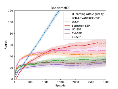
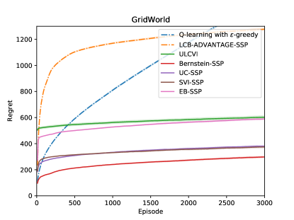
Figure 1: Accumulated regret of each algorithm on RandomMDP (left) and GridWorld (right) in $3000$ episodes. Each plot is an average of 500 repeated runs, and the shaded area is 95% confidence interval. Dotted lines represent model-free algorithms and solid lines represent model-based algorithms.

Table 3: Average time (in seconds) spent in updates in $3000$ episodes for each algorithm. Our model-based algorithm SVI-SSP is the most efficient algorithm.

	RandomMDP	GridWorld
Q-learning with $\epsilon$-greedy	0.3385	0.3773
LCB-Advantage-SSP	0.3517	0.3982
UC-SSP	14.4472	8.6886
Bernstein-SSP	0.2918	0.4656
ULCVI	15.7128	22.8062
EB-SSP	0.2319	0.4619
SVI-SSP	0.1207	0.1419

Table 4: Hyper-parameters used in the experiments. We search the best parameters for each algorithm.

	Algorithm	Parameters
RandomMDP	Q-learning with $\epsilon$-greedy	$\epsilon=0.05$
	LCB-Advantage-SSP	$H=5,\iota=0.05,\theta^{\star}=4096$
	UC-SSP	$\iota=1.0$
	Bernstein-SSP	$\iota=2.0$
	ULCVI	$H=80,\iota=2.0$
	EB-SSP	$\iota=0.05$
	SVI-SSP	$H=15,\iota=0.05$
GridWorld	Q-learning with $\epsilon$-greedy	$\epsilon=0.05$
	LCB-Advantage-SSP	$H=5,\iota=0.1,\theta^{\star}=4096$
	UC-SSP	$\iota=0.5$
	Bernstein-SSP	$\iota=0.5$
	ULCVI	$H=100,\iota=1.0$
	EB-SSP	$\iota=0.01$
	SVI-SSP	$H=10,\iota=0.01$

References

- Andrychowicz et al. [2017] Marcin Andrychowicz, Filip Wolski, Alex Ray, Jonas Schneider, Rachel Fong, Peter Welinder, Bob McGrew, Josh Tobin, OpenAI Pieter Abbeel, and Wojciech Zaremba. Hindsight experience replay. In Advances in Neural Information Processing Systems, volume 30, 2017.
- Azar et al. [2017] Mohammad Gheshlaghi Azar, Ian Osband, and Rémi Munos. Minimax regret bounds for reinforcement learning. In International Conference on Machine Learning, pages 263–272. PMLR, 2017.
- Bertsekas and Tsitsiklis [1991] Dimitri P Bertsekas and John N Tsitsiklis. An analysis of stochastic shortest path problems. Mathematics of Operations Research, 16(3):580–595, 1991.
- Bertsekas and Yu [2013] Dimitri P Bertsekas and Huizhen Yu. Stochastic shortest path problems under weak conditions. Lab. for Information and Decision Systems Report LIDS-P-2909, MIT, 2013.
- Chen and Luo [2021] Liyu Chen and Haipeng Luo. Finding the stochastic shortest path with low regret: The adversarial cost and unknown transition case. In International Conference on Machine Learning, 2021.
- Chen et al. [2021] Liyu Chen, Haipeng Luo, and Chen-Yu Wei. Minimax regret for stochastic shortest path with adversarial costs and known transition. In Conference On Learning Theory, 2021.
- Cohen et al. [2020] Alon Cohen, Haim Kaplan, Yishay Mansour, and Aviv Rosenberg. Near-optimal regret bounds for stochastic shortest path. In Proceedings of the 37th International Conference on Machine Learning, volume 119, pages 8210–8219. PMLR, 2020.
- Cohen et al. [2021] Alon Cohen, Yonathan Efroni, Yishay Mansour, and Aviv Rosenberg. Minimax regret for stochastic shortest path. In Neural Information Processing Systems, 2021.
- Efroni et al. [2019] Yonathan Efroni, Nadav Merlis, Mohammad Ghavamzadeh, and Shie Mannor. Tight regret bounds for model-based reinforcement learning with greedy policies. In Advances in Neural Information Processing Systems, volume 32. Curran Associates, Inc., 2019.
- Efroni et al. [2021] Yonathan Efroni, Nadav Merlis, Aadirupa Saha, and Shie Mannor. Confidence-budget matching for sequential budgeted learning. In International Conference on Machine Learning, 2021.
- Jaksch et al. [2010] Thomas Jaksch, Ronald Ortner, and Peter Auer. Near-optimal regret bounds for reinforcement learning. Journal of Machine Learning Research, 11(4), 2010.
- Jin et al. [2018] Chi Jin, Zeyuan Allen-Zhu, Sebastien Bubeck, and Michael I Jordan. Is Q-learning provably efficient? In Advances in neural information processing systems, pages 4863–4873, 2018.
- Jin et al. [2020] Chi Jin, Tiancheng Jin, Haipeng Luo, Suvrit Sra, and Tiancheng Yu. Learning adversarial Markov decision processes with bandit feedback and unknown transition. In Proceedings of the 37th International Conference on Machine Learning, pages 4860–4869, 2020.
- Lee et al. [2020] Chung-Wei Lee, Haipeng Luo, Chen-Yu Wei, and Mengxiao Zhang. Bias no more: high-probability data-dependent regret bounds for adversarial bandits and MDPs. In Advances in Neural Information Processing Systems, volume 33, pages 15522–15533. Curran Associates, Inc., 2020.
- Lim and Auer [2012] Shiau Hong Lim and Peter Auer. Autonomous exploration for navigating in MDPs. In Conference on Learning Theory, pages 40–1. JMLR Workshop and Conference Proceedings, 2012.
- Nasiriany et al. [2019] Soroush Nasiriany, Vitchyr Pong, Steven Lin, and Sergey Levine. Planning with goal-conditioned policies. In Advances in Neural Information Processing Systems, volume 32. Curran Associates, Inc., 2019.
- Neu et al. [2012] Gergely Neu, Andras Gyorgy, and Csaba Szepesvári. The adversarial stochastic shortest path problem with unknown transition probabilities. In Artificial Intelligence and Statistics, pages 805–813, 2012.
- Rosenberg and Mansour [2019] Aviv Rosenberg and Yishay Mansour. Online convex optimization in adversarial Markov decision processes. In Proceedings of the 36th International Conference on Machine Learning, pages 5478–5486, 2019.
- Rosenberg and Mansour [2020] Aviv Rosenberg and Yishay Mansour. Stochastic shortest path with adversarially changing costs. arXiv preprint arXiv:2006.11561, 2020.