Convergence of a Lagrangian–Eulerian scheme via weak asymptotic analysis for one-dimensional hyperbolic problems

Abstract

In this paper, we study both convergence and bounded variation properties of a new fully discrete conservative Lagrangian–Eulerian scheme to the entropy solution in the sense of Kruzhkov (scalar case) by using a weak asymptotic analysis. We discuss theoretical developments on the conception of no-flow curves for hyperbolic problems within scientific computing. The resulting algorithms have been proven to be effective to study nonlinear wave formations and rarefaction interactions. We present experiments to a study based on the use of the Wasserstein distance to show the effectiveness of the no-flow curves approach in the cases of shock interaction with an entropy wave related to the inviscid Burgers’ model problem and to a $2\times 2$ nonlocal traffic flow symmetric system of type Keyfitz–Kranzer.

1 Introduction

In this work, we present a fully discrete Lagrangian–Eulerian scheme, and its numerical analysis by a weak asymptotic method, for the computational treatment of first-order hyperbolic partial differential equations given by

$$\frac{\partial u}{\partial t}+\frac{\partial H(u)}{\partial x}=0,\quad x\in\mathbb{R},\quad t\in\mathbb{R}^{+},\quad\quad\quad u(x,0)=u_{0}(x),$$ (1.1)

where $u=u(x,t):\mathbb{R}\times\mathbb{R}^{+}\to\Omega\subset\mathbb{R}$ and $H:\Omega\to\mathbb{R}$.

To give a brief summary about the previous works that lead us to obtain the new method developed in this paper, we cite first [16]. In that article, an innovative locally conservative scheme was developed for the scalar parabolic convection-dominated convection–diffusion model problem of two-phase, immiscible, incompressible flow in porous media, the Locally Conservative Eulerian–Lagrangian Method (LCELM). This scheme was related to the divergence form of the parabolic flow equation, where the use of a space-time divergence form allowed the localization of the transport and the desired local conservation property could also be localized. Such a scheme was very competitive from a computational point of view for scalar nonlinear transport problems in heterogeneous porous media. To the best of our knowledge, the LCELM procedure was the first work in the literature to introduce a space-time local conservation (by physical and geometric arguments), a region where the mass conservation takes place (locally), which was coined as integral tube along with the so-called integral curves for scalar parabolic convection-diffusion models in porous media transport problems (see Eqs. (5.4a)-(5.4b) in [16]). Moreover, so-called integral curves were associated with points on the boundary (usually vertices) of the finite elements in that framework.

In this work, the fully discrete Lagrangian–Eulerian formulation is based on the new and substantial improvement interpretation of the integral tube, which is now subject to condition $O\left(\frac{H(u)}{u}\right)\propto\left[\frac{\Delta x}{\Delta t}\right]\to 0$ (called no-flow curves [7]), where the quantities $u$ and $H(u)$ come from the scalar initial value problem (1.1) and under a suitable stability estimate that is very effective in computing practice; as a result, we also obtain a weak CFL condition that does not depend on the derivative of the flux function $H(u)$, but only on the introduced no-flow curves. This simple and interesting technique is the key ingredient of the Lagrangian–Eulerian framework that provides information about the local wave propagation speed. This issue is not discussed in [16]. In addition, the no-flow curves reveal to be also a desingularization analysis tool for the construction of computationally stable schemes [6, 5, 7]. In [7], the authors also discussed a new reinterpretation of the Lagrangian–Eulerian no-flow curves as an anti-diffusion term into the viscosity coefficient defined by the quantity $O\left(\frac{H(u)}{u}\right)$, with a distinct identification to the Finite Volume framework. Here we are interested in the design of novel fully-discrete schemes based on the new concept no-flow curves subject to $O\left(\frac{H(u)}{u}\right)\propto\left[\frac{\Delta x}{\Delta t}\right]\to 0$ which is substantially different in theory foundations from the previous and relevant LCELM method.

The idea of how the fully discrete explicit locally conservative Lagrangian–Eulerian scheme works is outlined in the following three basic steps, for each time step, from $t^{n}$ to $t^{n+1}$. First, by using a space-time divergence form of model (1.1) we obtain an exact construction of the set of ODE modeling the so-called no-flow curves (see Figure 1). Second, by integrating the underlying conservation law (in divergence form) over the special region in the space-time domain (see region $D_{j}^{n,n+1}(x,t)$ in Figure 1), where the conservation of the mass flux takes place, we get the Lagrangian–Eulerian conservation relations. Third, by combining steps one and two, we perform an evolution (Lagrangian) step in time, from a primal grid to a nonstaggered grid and turn back by means of the final (Eulerian) projection step with a piecewise linear reconstruction (see Figure 2). A key hallmark of such method is the dynamic tracking forward of no-flow curves subject to $O\left(\frac{H(u)}{u}\right)\propto\left[\frac{\Delta x}{\Delta t}\right]\to 0$, per time step. The scheme is free of local Riemann problem solutions and does not use adaptive space-time discretization. This is a considerable improvement compared to the classical backward tracking over time of the characteristic curves over each time step interval, which is based on the strong form of the problem and that are not reversible for systems in general.

To analyze the properties of the explicit Lagrangian–Eulerian scheme, we use recent improvements on the weak asymptotic analysis (see [2, 3, 10]), which was first defined in a distinct framework by [13]. The weak asymptotic solutions are consistent with the traditional solutions in one-dimensional and multi-D (see also [2, 3, 5]). The weak asymptotic analysis has been used to study the existence of solutions for scalar equations and systems of hyperbolic equations, giving solutions a new meaning (see [2, 3, 11, 14, 12, 13, 15, 21, 22, 23, 25] and the references therein). An interesting aspect of this theory is that it makes it possible to prove the existence (and, for the scalar case, the uniqueness) of a solution by means of numerical methods.

In a previous work [5], we defined a weak asymptotic solution for a scalar equation (1.1) and outlined the proof of stability of the numerical method used. Weak asymptotic methods aim to investigate the nonlinear phenomena that appear in evolutionary equations (see [2, 3, 10]). In addition, they have been used in explicit calculations by several authors to study wave interactions inside the solutions to Riemann or Cauchy problems when these solutions involve nonclassical products of Heaviside functions, $\delta$-Dirac distributions, and even their derivatives. In [2], the authors show how one can construct families of continuous functions which asymptotically satisfy scalar equations with discontinuous nonlinearities and systems having irregular solutions. Through a weak asymptotic analysis, it has been proven, for scalar equations, that the initial value problem is well posed in the $L^{1}$ sense for the approximate solutions constructed. It was possible to demonstrate that the family of solutions obtained from the method satisfies Kruzhkov entropy, which provided a better understanding of the mathematical computations for the construction of accurate numerical schemes satisfying classical and entropy (Kruzhkov) solutions. It turns out that, beside the applications in nontrivial models of hyperbolic conservation laws, the convergent Lagrangian–Eulerian scheme via the weak asymptotic method treat such models with computational efficiency. From this theory, we obtain explicit estimates for the stability condition, and these estimates are numerically implemented and give very good numerical solutions as we see in the Section 4.

The proposed weak asymptotic analysis in this work, together with the Lagrangian–Eulerian approach [4, 5, 6, 7], fits in properly with the classical theory while improving the mathematical computations for the construction of new accurate numerical schemes, given by Proposition 3.1, where convergence, existence, and stability are established. In the classical treatment for proving convergence of a numerical scheme, first it is proved that the approximate solutions, generated by the numerical scheme, are of finite total variation (or bounded variation), actually, for scalar equations are proved that the total variation are not increasing. This condition gives the compact embedding of $BV$ functions in $L^{1}$; one can use the Helly’s selection theorem to show pointwise convergence of the generated sequence of solutions. After, it is proved that the generated sequence is a weak solution for the scalar equations and, finally, it is proved that the solution satisfies an entropy criterion, the most commom used is the Kruzhkov entropy condition, see [18]. The treatment used in the weak asymptotic analysis is very similar to the previous steps. To prove the main properties of the numerical scheme it is proved that the numerical scheme generates a solution with bounded total variation, also it is used a similar argument of Helly’s selection theorem, see Appendix C. Using the asymptotic theory, the solution to the proposed scheme is obtained as a family of functions, $\{u(\cdot,t,\epsilon)\}_{\epsilon}$, bounded in $\mathbb{L}^{1}(\mathbb{S}^{1})$ uniformly in parameter $\epsilon$ of the model (1.1)). The main difference is the kind of limit that is taken in solution in Equation $(\ref{weaksol})$. For instance, our approach allows us to deal with the reconstruction (accomplished by means of robust choices of slope limiters) of variable $u$ of Eq. $(\ref{noLi})$ in the (numerical) flux terms. We also give sufficient conditions for a total variation nonincreasing (Section 3.1) through a suitable semidiscrete formulation of Eq. $(\ref{noLi})$. In addition, we obtain the maximum principle and the entropy (Kruzhkov) solution to model $(\ref{noLi})$ thanks to a suitable interpretation of the approximate solutions provided by the analysis presented in Section 3.2. The weak asymptotic theory handles reconstructions easily and opens new possibilities for the design of new methods for hyperbolic problems under a weak CFL-type stability depending on the no-flow curves associated with the novel Lagrangian–Eulerian approach instead of using estimates on the eigenvalues, the weak asymptotic theory fits very well with the Lagragian-Eulerian scheme and it is a very promissor technique to be used to prove convergence for improved numerical methods of Lagrangian-Eulerian class.

The rest of this paper is structured as follows. Section 2 introduces the Lagrangian–Eulerian scheme. Section 3 presents the convergence of the numerical method via the weak asymptotic analysis. We propose a scheme to find a solution to $(\ref{noLi})$ and prove that the resulting solution converges to the weak solution of $(\ref{noLi})$. We demonstrate that the numerical scheme obtained in Section 2 is compatible with that used in the weak asymptotic analysis. Section 3.1 proves that our scheme has a total variation nonincreasing property for the solution. To complete our analysis, Section 3.2 demonstrates that the obtained solution satisfies the maximum principle and Kruzhkov entropy solution. Appendix A shows evidence that the reconstructions used in this study are Lipschitz continuous. Section 4 shows and discusses a set of representative computational results, including numerical studies with the W1 distance. Section 5 summarizes our concluding remarks.

2 Lagrangian–Eulerian scheme

To construct the fully discrete Lagrangian–Eulerian scheme, we first consider the scalar one-dimensional (1D) Cauchy problem (1.1) in its divergent form

$$\nabla\cdot\left[\begin{array}[]{c}H(u)\\ u\end{array}\right]=0,\quad t>0,\quad x\in\mathbb{R},\qquad u(x,0)=u_{0}(x),\quad x\in\mathbb{R},\quad\text{ where }\nabla=\left(\frac{\partial}{\partial x},\frac{\partial}{\partial t}\right).$$ (2.1)

For the sake of clarity and completeness, we sketch in what follows the main three steps of the Lagrangian–Eulerian approach, namely, the construction of the set of ODE modeling the no-flow curves (Section 2.1), the Lagrangian–Eulerian conservation relations (Section 2.2) and the final projection step by piecewise linear reconstruction (Section 2.3), along with an evolution algorithm of the fully discrete nonstaggered Lagrangian-Eulerian method. As in the Lagrangian–Eulerian schemes present in [4, 5, 6, 7], local conservation is obtained by integrating the conservation law over the region in the space-time domain where the conservation of mass flux takes place.

2.1 Lagrangian–Eulerian no-flow curves

Consider the Lagrangian–Eulerian control volumes

$${D_{j}^{n,n+1}}=\{(x,t)\,\,/\,\,\sigma^{n}_{j-\frac{1}{2}}(t)\leq x\leq\sigma^{n}_{j+\frac{1}{2}}(t),\,\,t^{n}\leq t\leq t^{n+1}\},$$ (2.2)

where $\sigma_{j\pm\frac{1}{2}}^{n}(t)$ are the Lagrangian–Eulerian no-flow curves such that $\sigma_{j\pm\frac{1}{2}}^{n}(t^{n})=x_{j\pm\frac{1}{2}}^{n}$ and subject to $O\left(\frac{H(u)}{u}\right)\propto\left[\frac{\Delta x}{\Delta t}\right]\to 0$ [5, 6, 7] along with $u$ and $H(u)$ given from (2.1). These curves correspond to the lateral boundaries of domain ${D_{j}^{n,n+1}}$ in (2.2), and we define $\bar{x}_{j\pm\frac{1}{2}}^{n}:=\sigma_{j\pm\frac{1}{2}}^{n}(t^{n+1})$ as their endpoints in time $t^{n+1}$. For each control volume, $h_{j}^{n}$ is defined as $h_{j}^{n}=x_{j+\frac{1}{2}}^{n}-x_{j-\frac{1}{2}}^{n}$.

The numerical scheme is expected to satisfy certain type of mass conservation (due to the inherent nature of the conservation law) from time $t^{n}$ in the space domain $[x_{j-\frac{1}{2}}^{n},x_{j+\frac{1}{2}}^{n}]$ to time $t^{n+1}$ in the space domain $[\bar{x}_{j-\frac{1}{2}}^{n+1},\bar{x}_{j+\frac{1}{2}}^{n+1}]$; see also [16] for original motivation foundations on models for the flow of fluids and the transport of mass conservation in porous geologic media. Based on this, the flux through curves $\sigma_{j\pm\frac{1}{2}}^{n}(t)$ must be zero. With the integration of (1.1) and the Divergence Theorem, and because the line integrals over curves $\sigma_{j\pm\frac{1}{2}}^{n}(t)$ vanish,

$$\int_{\bar{x}_{j-\frac{1}{2}}^{n+1}}^{\bar{x}_{j+\frac{1}{2}}^{n+1}}u(x,t^{n+1})dx=\int_{x_{j-\frac{1}{2}}^{n}}^{x_{j+\frac{1}{2}}^{n}}u(x,t^{n})dx.$$ (2.3)

Here curves $\sigma_{j\pm\frac{1}{2}}^{n}(t)$ are not straight lines in general but rather solutions to the set of local nonlinear differential equations (as in [7, 6] for systems): $\frac{d}{dt}[\sigma_{j\pm\frac{1}{2}}^{n}(t)]=\frac{H(u)}{u}$, for $t^{n}<t\leq t^{n+1},$ with the initial condition $\sigma_{j\pm\frac{1}{2}}^{n}(t^{n})=x_{j\pm\frac{1}{2}}^{n}$, assuming $u\neq 0$ (for the sake of presentation). This construction follows naturally from the finite volume formulation of the linear Lagrangian–Eulerian scheme (see Figure 1) as a building block to construct local approximations for $\frac{H(u)}{u}$, such as $f_{j\pm\frac{1}{2}}^{n}=\frac{H(U_{j\pm\frac{1}{2}}^{n})}{U_{j\pm\frac{1}{2}}^{n}}$, with the initial condition $\sigma_{j\pm\frac{1}{2}}^{n}(t^{n})=x_{j\pm\frac{1}{2}}^{n}$.

Remark 2.1.

In fact, distinct and high-order approximations are also acceptable for $\frac{d}{dt}[\sigma_{j\pm\frac{1}{2}}^{n}(t)]$ and can be regarded as ingredients to improve the accuracy of the new family of Lagrangian–Eulerian methods.

Eq. (2.3) defines the mass conservation but in a different mesh cell-centered in points $\bar{x}_{j+\frac{1}{2}}^{n}$ of width $h_{j}^{n+1}$ defined by $h^{n+1}_{j}=h^{n}_{j}+(f^{n}_{j+\frac{1}{2}}-f^{n}_{j-\frac{1}{2}})\Delta t$, which gives us $\frac{h^{n}_{j}}{h^{n+1}_{j}}=1-\frac{{f^{n}_{j+\frac{1}{2}}-f^{n}_{j-\frac{1}{2}}}}{{h^{n+1}_{j}}}\Delta t.$ Along the linear approximations of $f_{j\pm\frac{1}{2}}^{n}$, we have that $\bar{x}_{j\pm\frac{1}{2}}=x_{j\pm\frac{1}{2}}+f^{n}_{j\pm\frac{1}{2}}\Delta t$.

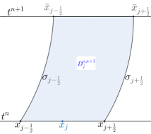
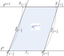
Figure 1: Left: No flow region ${D_{j}^{n,n+1}}$. Right: Linear approximation for ${D_{j}^{n,n+1}}$.

2.2 Conservation relations

Equation (2.3) defines a local mass balance between space intervals at times $t^{n}$ and $t^{n+1}$. By defining

$$\overline{U}_{j}^{n+1}:=\frac{1}{h_{j}^{n+1}}\int_{\bar{x}_{j-\frac{1}{2}}^{n+1}}^{\bar{x}_{j+\frac{1}{2}}^{n+1}}u(x,t^{n+1})dx,\quad\text{and}\quad U_{j}^{n}:=\frac{1}{h^{n}_{j}}\int_{x_{j-\frac{1}{2}}^{n}}^{x_{j+\frac{1}{2}}^{n}}u(x,t^{n})dx,$$

the discrete version of Eq. (2.3) is given by

$$\overline{U}_{j}^{n+1}=\frac{1}{h_{j}^{n+1}}\int_{\bar{x}_{j-\frac{1}{2}}^{n+1}}^{\bar{x}_{j+\frac{1}{2}}^{n+1}}u(x,t^{n+1})dx=\frac{1}{h_{j}^{n+1}}\int_{x_{j-\frac{1}{2}}^{n}}^{x_{j+\frac{1}{2}}^{n}}u(x,t^{n})dx=\frac{h^{n}_{j}}{h_{j}^{n+1}}U_{j}^{n}.$$ (2.4)

Solutions $\sigma_{j\pm\frac{1}{2}}^{n}(t)$ to the differential system are also obtained using linear approximations $L(x,t)$. A piecewise constant numerical data is reconstructed into a piecewise linear approximation (although high-order reconstructions are acceptable) by means of MUSCL-type interpolants $L_{j}(x,t)=u_{j}(t)+(x-x_{j})\frac{1}{h^{n}_{j}}u^{\prime}_{j}$.

Remark 2.2.

For the numerical derivative $\frac{1}{h^{n}_{j}}u^{\prime}_{j}$, there are many choices of slope limiters (see, e.g., [6, 4]). Even though selecting such slope limiters a priori is quite hard, this choice is based on the underlying model problem under study.

The approximation of $U^{n}_{j-\frac{1}{2}}$ is

$$\begin{array}[]{ll}U^{n}_{j-\frac{1}{2}}&=\frac{1}{h^{n}_{j}}\int_{x_{j-1}^{n}}^{x_{j}^{n}}L(x,t)dx=\frac{1}{h^{n}_{j}}\left(\int_{x_{j-1}^{n}}^{x_{j-\frac{1}{2}}^{n}}L_{j-1}(x,t)dx+\int_{x_{j-\frac{1}{2}}^{n}}^{x_{j}^{n}}L_{j}(x,t)dx\right)\\ \\ &=\frac{1}{2}(U^{n}_{j-1}+U^{n}_{j})+\frac{1}{8}({U_{j}^{n}}^{\prime}-{U_{j-1}^{n}}^{\prime}).\end{array}$$ (2.5)

2.3 Projection step

Next, for a partition with constant spacing ($h^{n}_{j}=h,\forall j$), we obtain the resulting projection formula as follows:

$$U_{j}^{n+1}=\frac{1}{h}\left(c_{-1,j}\overline{U}_{j-1}^{n+1}+c_{0,j}\overline{U}_{j}^{n+1}+c_{+1,j}\overline{U}_{j+1}^{n+1}\right),$$ (2.6)

where the projection coefficients are

$$c_{-1,j}=f^{+}(U^{n}_{j-\frac{1}{2}})\Delta t,\quad c_{+1,j}=f^{-}(U^{n}_{j+\frac{1}{2}})\Delta t,\quad c_{0,j}=h-c_{-1,j}-c_{+1,j},$$ (2.7)

and $f^{+}$, $f^{-}$ defined as

$$f^{+}=\max(f,0)\quad\text{ and }\quad f^{-}=\max(-f,0).$$ (2.8)

Figure 2: Projection to original mesh.

Note that, for function $f$, we have $f=f^{+}-f^{-}$ and $|f|=f^{+}+f^{-}.$ Here $\Delta t$ is obtained under a weak CFL condition, that does not depend on the derivative of the flux function $H(u)$, but only based in the so-called no-flow curves $f^{n}_{j-\frac{1}{2}}$,

$${\max_{j}\left\{|f^{n}_{j-\frac{1}{2}}\,\Delta t|\right\}\leq\frac{h}{2},}$$ (2.9)

which is taken by construction of the method. We note that, in the linear case, when $a(x,t)=a>0$ (or $a<0$), numerical scheme (2.4)–(2.6) is a generalization of the upwind scheme. However, our scheme can provide an approximate solution in both scenarios: $a>0$ and $a<0$. In this case, the CFL condition is $|a\,\Delta t|\leq h$, as in the upwind scheme. For the sake of clarity and completeness, we include the numerical experiment with the sonic rarefaction for the invicid Burgers’ problem. Here, as the rarefaction wave is crossed, there is a sign change in the characteristic speed $u$, in the range $-1<u<1$ and thus there is one point at which $u=0$, the sonic point. Our approach does not use Riemann solvers neither Godunov type implementation. We can summarize the ideas presented so far in the following algorithm.

Algorithm Nonstaggered Lagrangian-Eulerian method

procedure NSLEstep($h^{n}$, $U^{n}$, $t^{n}$, $t^{n+1}$)

     1. Approximate the no-flow boundaries slope with $f_{j+\frac{1}{2}}^{n}\leftarrow\frac{H(U^{n}_{j+\frac{1}{2}})}{U^{n}_{j+\frac{1}{2}}}$.

     2. Find the new mesh $h_{j}^{n+1}\leftarrow h_{j}^{n}+(f_{j+\frac{1}{2}}-f_{j-\frac{1}{2}})\Delta t$.

     3. Compute the conserved quantity $\overline{U}_{j}^{n+1}$ with (2.4);

     4. Compute $U^{n}_{j-\frac{1}{2}}$ using an appropriate slope limiter with (2.5).

     5. Compute the projection coefficients $c_{-1,j},c_{0,j}$ and $c_{+1,j}$ with (2.7).

     return the values $U^{n+1}_{j}$ projected from $\overline{U}_{j}^{n+1}$ into the original mesh with (2.6).

We now examine the theoretical properties of the Lagrangian–Eulerian scheme via weak asymptotic solutions.

2.4 Slope limiters

States $U^{n}_{j-\frac{1}{2}}$ are obtained from states $U^{n}_{j-1}$ and $U^{n}_{j}$ and functions $U^{\prime}_{j-1}$ and $U^{\prime}_{j}$ in timestep $n$. These functions (obtained using slope limiters) compute variations of function $U$ at the neighborhood of $U_{j-\frac{1}{2}}$. We would like to stress that said functions ($U^{\prime}_{j-1}$ and $U^{\prime}_{j}$) are not numerical derivatives because they can compute variations even for noncontinuous $U$. In Appendix A, we demonstrate that they are Lipschitz continuous. The first option of slope limiter is

$$U^{\prime}_{j}=\text{MM}_{2}\left(\Delta u_{j+\frac{1}{2}},\Delta u_{j-\frac{1}{2}}\right),$$ (2.10)

where $\text{MM}_{2}$ corresponds to the most common limiter (see, e.g., [4, 5]), with $\Delta u_{j+\frac{1}{2}}=u_{j+1}-u_{j}$, and can be written as

$$\text{MM}_{2}\left(\sigma,\tau\right)=\frac{1}{2}\lambda(\sigma,\tau)\min\left(|\sigma|,|\tau|\right),$$ (2.11)

where $\lambda(u,v)=\text{sgn}(u)+\text{sgn}(v)$. The following option, which allows steeper slopes near discontinuities and retains accuracy in smooth regions (obtained between three values), can also be used and is given by

$$U^{\prime}_{j}=\text{MM}_{3}\left(\alpha\Delta u_{j+\frac{1}{2}},\frac{1}{2}(u_{j+1}-u_{j-1}),\alpha\Delta u_{j-\frac{1}{2}}\right),$$ (2.12)

where $\text{MM}_{3}$ can be written as

$$\text{MM}_{3}\left(\sigma,\tau,\gamma\right)=\frac{1}{8}\lambda(\sigma,\tau)\lambda(\sigma,\gamma)\lambda(\tau,\gamma)\min\left(|\sigma|,|\gamma|,|\tau|\right),$$ (2.13)

One can prove that $\text{MM}_{3}(x,y,z)=\text{MM}_{2}\left(\text{MM}_{2}(x,y),z\right).$ A third option is the high-order slope limiter UNO, which is given by

$$U^{\prime}_{j}=\text{MM}_{2}\left(\Delta u_{j+\frac{1}{2}}-\delta^{2}_{1},\Delta u_{j-\frac{1}{2}}+\delta^{2}_{2}\right),$$ (2.14)

where $\delta^{2}_{1}$ is a function of $u_{j+2}$, $u_{j+1}$, $u_{j}$ and $u_{j-1}$ defined by $\delta^{2}_{1}=\frac{1}{2}\text{MM}\left(\Delta^{2}u_{j+1},\Delta^{2}u_{j}\right)$; and $\delta^{2}_{2}$, of $u_{j+1}$, $u_{j}$, $u_{j-1}$ and $u_{j-2}$ defined by $\delta^{2}_{2}=\frac{1}{2}\text{MM}\left(\Delta^{2}u_{j},\Delta^{2}u_{j-1}\right)$ and $\Delta^{2}u_{j}=u_{j+1}-2u_{j}+u_{j-1}$. In Appendix A, we demonstrate that the reconstructions of $U_{j+\frac{1}{2}}$ are Lipschitz continuous.

3 The convergence proof of the Lagrangian–Eulerian scheme

In the classical treatment for proving convergence of a numerical scheme, first it is proved that the approximate solutions, generated by the numerical scheme, are of finite total variation (or bounded variation), actually, for scalar equations are proved that the total variation are not increasing. This condition gives the compact embedding of $BV$ functions in $L^{1}$, one can use the Helly’s selection theorem to show compactness for the approximations and establish pointwise convergence. After, it is proved that the solution is a weak solution for the scalar equations and, finally, it is proved that the solution satisfies an entropy criterion, the most commom used is the Kruzhkov entropy condition, see [18]. In this Section, we show the convergence of our scheme using the weak asymptotic theory, that is very suitable to handle with the Eulerian-Lagrangian approach. From this theory, we obtain explicit estimates for the stability condition, these estimates are implemented and give very good numerical solutions as one can see in the Section 4.

To establish the weak asymptotic solution, we consider the one-dimensional scalar equation in (1.1). In order to avoid boundary conditions in the bounded domain due to numerical purposes, we consider that $x\in\mathbb{S}^{1}=\mathbb{R}/\mathbb{Z}$; variable $t\in\mathbb{R}^{+}$, thus $u=u(x,t):\mathbb{S}^{1}\times\mathbb{R}^{+}\to\Omega\subset\mathbb{R}$, and the flux function $H=H(u):\Omega\to\mathbb{R}$ is assumed to be a locally Lipschitz function in $u$, i.e.,

Assumption 1 - for all $c>0$, $\exists L>0$, such that

$$|u_{1}|\leq c,|u_{2}|\leq c\Longrightarrow|H(u_{1})-H(u_{2})|\leq L|u_{1}-u_{2}|.$$ (3.1)

The weak asymptotic solution is a sequence of solutions $(u_{\epsilon})_{\epsilon}=(u(x,t,\epsilon))_{\epsilon}$ of class $\mathcal{C}^{1}$ in $t$ and class $L^{\infty}$ and is piecewise continuous in $x$ such that, for all $\psi=\psi(x)\in\mathcal{C}^{\infty}_{c}(\mathbb{R})$ (smooth with compact support), and, for all $t$,

$$\lim_{\epsilon\to 0}\int_{R}((u_{\epsilon})_{t}\psi-H(u_{\epsilon})\psi_{x})dx=0\quad\text{and}\quad u_{\epsilon}(x,0)=u_{0}(x).$$ (3.2)

In the weak asymptotic method, a PDE with a special flux (using parameter $\epsilon$) is first proposed. Then, for each fixed $\epsilon$, we obtain an Ordinary Differential Equation (ODE) for variable $t$. Based on the theory of ODEs, we prove the existence and stability of the solution. Finally, we demonstrate that, when taking $\epsilon\to 0$, the limit satisfies (3.2). The idea is for the flux to represent the numerical method, which is why the existence and stability of the PDE with special class may be an extension of the numerical method. In our method, we use an auxiliary function ($f(u)=H(u)/u$) and assume that $u\neq 0$ to avoid technical details (we would like to stress that the convergence of the method can be proven in this case). Moreover, we assume that there exists a $a>0$ such that $u>a>0$. Note that, in this case, $f(u)$ is a locally Lipschitz function in $u$ because for all $c>a$, $\exists\tilde{K}>0$ such that

$$a<u_{1}\leq c,\;a<u_{2}\leq c\Longrightarrow|f(u_{1})-f(u_{2})|\leq\tilde{K}|u_{1}-u_{2}|.$$

Notice that we can take $\tilde{K}=L/a+\tilde{M}_{c}/a^{2}$, where $\displaystyle{\tilde{M}_{c}=\max_{a<u\leq c}|H(u)|}$.

For our method, we propose the following ODE:

$$\partial_{t}(u_{{}_{\epsilon}})=\frac{1}{\epsilon}\left[u_{{}_{\epsilon-1}}f^{+}(\hat{u}_{{}_{\epsilon-1/2}})-u_{{}_{\epsilon}}f^{+}(\hat{u}_{{}_{\epsilon+1/2}})-u_{{}_{\epsilon}}f^{-}(\hat{u}_{{}_{\epsilon-1/2}})+u_{{}_{\epsilon+1}}f^{-}(\hat{u}_{{}_{\epsilon+1/2}})\right],$$ (3.3)

with initial condition $u_{\epsilon}(x,0)=u_{0}(x,0)$. Here $f^{+}$ and $f^{-}$ are defined in $(\ref{fmm})$ and $u_{{}_{\epsilon-i}}$, $u_{{}_{\epsilon+i}}$, and $u_{{}_{\epsilon}}$ are defined as $\displaystyle{u_{{}_{\epsilon-i}}=u(x-i\epsilon,t,\epsilon)}$, $\displaystyle{u_{{}_{\epsilon+i}}=u(x+i\epsilon,t,\epsilon)}$ and $\displaystyle{u_{{}_{\epsilon}}=u(x,t,\epsilon)}$. Functions ${f^{+}\left(\hat{u}_{{}_{\epsilon-1/2}}\right)}$ and $f^{-}\left(\hat{u}_{{}_{\epsilon-1/2}}\right)$ are evaluated in the middle of each cell, i.e, they are given by following identities ${f^{+}\left(\hat{u}_{{}_{\epsilon-1/2}}\right)=f^{+}\left(\hat{u}_{{}_{\epsilon-1/2}},x-\frac{\epsilon}{2},t\right)}$,
${f^{+}\left(\hat{u}_{{}_{\epsilon+1/2}}\right)=f^{+}\left(\hat{u}_{{}_{\epsilon+1/2}},x+\frac{\epsilon}{2},t\right)}$, ${f^{-}\left(\hat{u}_{{}_{\epsilon-1/2}}\right)=f^{-}\left(\hat{u}_{{}_{\epsilon-1/2}},x-\frac{\epsilon}{2},t\right)},$ and ${f^{-}\left(\hat{u}_{{}_{\epsilon+1/2}}\right)=f^{-}\left(\hat{u}_{{}_{\epsilon+1/2}},x+\frac{\epsilon}{2},t\right)}$.

States $\hat{u}_{{}_{\epsilon-1/2}}$ and $\hat{u}_{{}_{\epsilon+1/2}}$ are obtained from a combination of known states from equations such as $(\ref{umeio})$ and are also determined in the middle of each cell. For the general case, we assume that there is a function $L(x_{-p},\dots,x_{p})$ so that we can define, for instance, $\hat{u}_{{\epsilon+1/2}}$ as:

$$\hat{u}_{{\epsilon+1/2}}=L(u(x-p\epsilon,t,\epsilon),u(x-(p-1)\epsilon,t,\epsilon),\dots,u(x+(p-1)\epsilon,t,\epsilon),u(x+p\epsilon,t,\epsilon)).$$ (3.4)

Function $L$ is generated using the slope limiters (defined in Section 2.4). In addition, we assume the following compatibility condition: for any $x$, $x=L(x,x,\dots,x).$ In Appendix A, we prove that the slope limiters, as well as the reconstructions of type $(\ref{umeio})$, are Lipschitz continuous. In this case, if $u(x+i\epsilon,t,\epsilon)$ are continuous functions

$$\lim_{\epsilon\longrightarrow 0}|u_{\epsilon}-\hat{u}_{\epsilon-1/2}|=\lim_{\epsilon\longrightarrow 0}|u_{\epsilon}-\hat{u}_{\epsilon+1/2}|=0.$$ (3.5)

Note that since $f(u)$ and $L$ are Lipschitz continuous, then $f$ applied to $\hat{u}_{{}_{\epsilon-1/2}}$ is also a Lipschitz function.

In the next result, we state the existence and stability result of the solution to $(\ref{ODE})$. As strategy of proof, we apply the Taylor expansion with remainder term to substitute the derivative by a difference defined between $t$ and $t+dt$, where $dt$ represents a time step. We state our result as follows:

Proposition 3.1.

We construct, as a solution to $(\ref{ODE})$, a family of functions $(x,t)\to u(x,t,\epsilon):\mathbb{S}^{1}\times\mathbb{R}\to\mathbb{R}$, for small enough $\epsilon$, that are of class $\mathbb{C}^{1}$ in $t$ for a fixed $\epsilon$ and of class $\mathbb{L}^{\infty}$ for $x\in\mathbb{S}^{1}$ and satisfy $(\ref{weaksol})$. If

$$\frac{dt}{\epsilon}\left(f^{+}\left(\hat{u}_{{}_{\epsilon+1/2}}\right)+f^{-}\left(\hat{u}_{{}_{\epsilon-1/2}}\right)\right)\leq 1,\quad\text{ for all }\quad\hat{u}_{{}_{\epsilon-1/2}}\text{ and }\hat{u}_{{}_{\epsilon+1/2}}$$ (3.6)

is satisfied, then the family $\{u(\cdot,t,\epsilon)\}_{\epsilon}$ is bounded in $\mathbb{L}^{1}(\mathbb{S}^{1})$ uniformly in $\epsilon$. In fact, we have that $||u(t,\epsilon)||_{\mathbb{L}^{1}(\mathbb{S}^{1})}\leq||u_{0}||_{\mathbb{L}^{1}(\mathbb{S}^{1})}$ for all $t$. Moreover, if initial condition $u_{0}(x)$ and $H(u)$ are continuous, then $u(x,t,\epsilon)$ is also continuous in $x$.

Notice that $(\ref{Cflcon})$ is always valid if the CFL condition $(\ref{CFL})$ is satisfied. Indeed, the proof of Proposition 3.1 follows ideas from works [2, 3, 10], however, here is the first time that we prove the result for reconstructions of variable $u(x,t)$. Moreover, with the adaptation of our proof, we are able to obtain new conditions to guarantee the stability of the numerical method. These conditions are not obtained in previous works.

Proof. First, we fix $\epsilon$ and obtain an ODE from (3.3) for variable $t$ as follows:

$${u}^{\prime}(x,t,\epsilon)=F_{\epsilon}({u}(x,t,\epsilon)),\quad{u}(0,x)=u_{0}(x),$$ (3.7)

Notice that $x$ is also a parameter in Eq. $(\ref{xxt})$. We define $F_{\epsilon}:L^{\infty}(\mathbb{S}^{1})\longrightarrow L^{\infty}(\mathbb{S}^{1})$ as

$$F_{\epsilon}(u_{\epsilon}(x,t),x,t)=\frac{1}{\epsilon}\Big{[}u(x-\epsilon,t,\epsilon)f^{+}\left(\hat{u}\left(x-\frac{\epsilon}{2},t,\epsilon\right),x-\frac{\epsilon}{2},t\right)$$

$$-u(x,t,\epsilon)f^{+}\left(\hat{u}\left(x+\frac{\epsilon}{2},t,\epsilon\right),x+\frac{\epsilon}{2},t\right)-u(x,t,\epsilon)f^{-}\left(\hat{u}\left(x-\frac{\epsilon}{2},t,\epsilon\right),x-\frac{\epsilon}{2},t\right)$$

$$+u\left(x+{\epsilon},t,\epsilon\right)f^{-}\left(\hat{u}\left(x+\frac{\epsilon}{2},t,\epsilon\right),x+\frac{\epsilon}{2},t\right)\Big{]}$$ (3.8)

Here $\hat{u}\left(x+{\epsilon/2},t,\epsilon\right)$ is obtained from reconstruction $L(x_{-p},\dots,x_{p})$ as in Eq. $(\ref{ffdse})$:

$$\begin{split}\hat{u}(x+{\epsilon/2},t,\epsilon)=L(u(x-p\epsilon,t,\epsilon),\dots u(x+(p-1)\epsilon,t,\epsilon),u(x+p\epsilon,t,\epsilon)).\end{split}$$ (3.9)

Since $f(\cdot)$ and reconstruction $L(x_{-p},\dots,x_{p})$ are Lipschitz continuous, so are $f(L(x_{-p},\dots,x_{p}))$. Since flux $F_{\epsilon}$, defined in Eq. $(\ref{fluxeps})$, is a combination of Lipschitz continuous (in a remarkably simple way), we get that $F_{\epsilon}$ is also a Lipschitz function. Thus, based on the classical theory of ODEs in Banach spaces, in the Lipschitz continuous case, there is a local solution to $t\in[0,\delta(\epsilon)]$ for some $\delta(\epsilon)$ that depends on $\epsilon$. For the global solution, since $f$ is bounded (because $H$ is assumed to be Lipschitz continuous), we can extend the solution to $\delta(\epsilon)\to\infty$. From assumption 1, Eq. $(\ref{h1})$, the Lipschitz constants of each $F_{\epsilon}$ can be chosen uniformly on bounded sets $L^{\infty}({\mathbb{S}^{1}})\times[0,\infty)$. To demonstrate the existence of the solution $(\ref{xxt})$ globally (in time), it suffices to prove that, for fixed $\epsilon$, there exists a $c_{\epsilon}(t)<\infty$ such that $||u(\cdot,t,\epsilon)||_{\infty}\leq c_{\epsilon}(t)<\infty$. Here $c_{\epsilon}$ is a continuous function on $[0,\infty)$, which is not uniformly continuous in $\epsilon$. We also have that $H(u)$ is a bounded function; hence, if $u\geq a>0$, then $f$ is also bounded. Let $M$ be defined as

$$M=\sup_{\begin{array}[]{c}(u,x,t)\in\Omega\times[0,T]\times{\mathbb{S}^{1}}\end{array}}|f(u,x,t)|<\infty.$$

We have that $\displaystyle{|\partial_{t}u(x,t,\epsilon)|\leq\frac{4}{\epsilon}||u(\cdot,t,\epsilon)||_{\infty}M}$ where $\displaystyle{||u(\cdot,t,\epsilon)||_{\infty}=\text{ess}\sup_{x\in{\mathbb{S}^{1}}}|u(x,t,\epsilon)|}$. Solving, we obtain:

$$||u(\cdot,t,\epsilon)||_{\infty}\leq||u_{0}(\cdot)||_{\infty}+\frac{4M}{\epsilon}\int_{0}^{t}||u(\cdot,\tau,\epsilon)||_{\infty}d\tau.$$

From Grönwall formula, we obtain that:

$$||u(\cdot,t,\epsilon)||_{\infty}\leq c_{\epsilon}(t),\quad\text{ where }\quad c_{\epsilon}(t)=||u_{0}(\cdot)||_{\infty}\exp\left(\frac{4Mt}{\epsilon}\right).$$ (3.10)

Bound $(\ref{ggr})$ indicates the existence of a global solution to the ODE $(\ref{ODE})$ for each fixed $\epsilon$. However, note that the solutions to the system of ODEs are not uniformly continuous in $\epsilon$. To demonstrate that the solutions to ODEs provide a weak asymptotic solution for $(\ref{noLi})$, we will prove that the solution is $L^{1}$ bounded uniformly with respect to $\epsilon$. To do so, let $T>0$ for $t+dt\leq T$ and $dt>0$. From the Taylor expansion with remainder term (for fixed $\epsilon)$, it follows that $(\ref{ODE})$ can be written as

$$u(x,t+dt,\epsilon)=u_{\epsilon} +\frac{dt}{\epsilon}\left[u_{{}_{\epsilon-1}}f^{+}\left(\hat{u}_{{}_{\epsilon-1/2}}\right)-u_{{}_{\epsilon}}f^{+}\left(\hat{u}_{{}_{\epsilon+1/2}}\right)-u_{{}_{\epsilon}}f^{-}\left(\hat{u}_{{}_{\epsilon-1/2}}\right)\right.$$

$$\left.+u_{{}_{\epsilon+1}}f^{-}\left(\hat{u}_{{}_{\epsilon+1/2}}\right)\right]+dt\;r(x,t,\epsilon,dt),$$

where $||r(\cdot,t,\epsilon,dt)||_{1}\to 0$ (or $||r(\cdot,t,\epsilon,dt)||_{\infty}\to 0$), uniformly in $t\in[0,T]$ and fixed $\epsilon$ (and not uniformly continuous in $\epsilon$), when $dt\to 0$. This behavior results from the continuous differentiability of map $t\longrightarrow u(\cdot,t,\epsilon)$, $[0,\infty)\longrightarrow L^{\infty}({\mathbb{S}^{1}})$ for fixed $\epsilon$. Since we are interested in obtaining the $L^{1}$ bound, we take the absolute value,

$$|u(x,t+dt,\epsilon)|\leq |u_{\epsilon}|\left(1-\frac{dt}{\epsilon}(f^{+}\left(\hat{u}_{{}_{\epsilon+1/2}}\right)+f^{-}\left(\hat{u}_{{}_{\epsilon-1/2}}\right)\right)+\frac{dt}{\epsilon}\left[|u_{{}_{\epsilon-1}}|f^{+}\left(\hat{u}_{{}_{\epsilon-1/2}}\right)\right]$$

$$+\frac{dt}{\epsilon}\left[|u_{{}_{\epsilon+1}}|f^{-}\left(\hat{u}_{{}_{\epsilon+1/2}}\right)\right]+dt|r(x,t,dt)|.$$ (3.11)

From the definition of $f^{+}$ and $f^{-}$ in Eq. (2.7), we get that if $(\ref{Cflcon})$ is satisfied, then $(\ref{ODE2n})$ is true. Notice that $(\ref{Cflcon})$ is always valid if the CFL condition $(\ref{CFL})$ is satisfied. This proves that the condition $(\ref{CFL})$ provides the method with stability because by integrating $(\ref{ODE2n})$ and the appropriate translations of $\pm\epsilon$, we obtain

$$||u(\cdot,t+dt,\epsilon||_{1}=\int_{\mathbb{S}^{1}}|u(x,t+dt,\epsilon)|dx\leq\int_{\mathbb{S}^{1}}|u(x,t,\epsilon)|dx+dt\;r_{1}(t,\epsilon,dt).$$ (3.12)

Here the remainder value $r_{1}(t,\epsilon,dt)=\int_{\mathbb{S}}|r(\cdot,t,\epsilon,dt)|dx$ is bounded, and $r_{1}(t,\epsilon,dt)\to 0$ when $dt\to 0$, uniformly in $t\in[0,T]$ for each fixed $\epsilon$. Notice that, for each $T>0$ given, we can divide interval $[0,T]$ into $n$ subintervals $[jdt_{n},(j+1)dt_{n}]$, where $dt_{n}=\frac{T}{n}$ and $0\leq j\leq n-1$. Applying this in $(\ref{fdsee})$, we get

$$\int_{\mathbb{S}^{1}}|u(x,T,\epsilon)|dx\leq\int_{\mathbb{S}^{1}}|u(x,T-dt_{n},\epsilon)|dx+dt_{n}\;r_{1}(T-dt,\epsilon,dt).$$

Applying recursively for all intervals, we obtain

$$\int_{\mathbb{S}^{1}}|u(x,T,\epsilon)|dx\leq\int_{\mathbb{S}^{1}}|u_{0}(x)|dx+dt_{n}\;\sum_{i=1}^{n}r_{1}(T-idt,\epsilon,dt).$$

Notice that

$$dt_{n}\;\left|\sum_{i=1}^{n}r_{1}(T-idt,\epsilon,dt)\right|\leq\frac{T}{n}n\max_{i}|r_{1}(T-idt,\epsilon,dt)|=T\max_{i}|r_{1}(T-idt,\epsilon,dt)|.$$

Thus, taking the limit $dt\longrightarrow 0$ and using $r_{1}(t,\epsilon,dt)\longrightarrow 0$, when $dt\longrightarrow 0$ we obtain:

$$||u(\cdot,T,\epsilon)||_{1}=\int_{\mathbb{S}^{1}}|u(x,T,\epsilon)|dx\leq\int_{\mathbb{S}^{1}}|u_{0}(x)|dx=||u_{0}(\cdot)||_{1},$$ (3.13)

which gives us the $L^{1}$ uniform bounds in $\epsilon$.

To complete the proof of the proposition, we define integral $I$ as

$$I=\int_{{\mathbb{S}^{1}}}\left(\frac{1}{\epsilon}\left[u_{{}_{\epsilon-1}}f^{+}\left(\hat{u}_{{}_{\epsilon-1/2}}\right)-u_{{}_{\epsilon}}f^{+}\left(\hat{u}_{{}_{\epsilon+1/2}}\right)-u_{{}_{\epsilon}}f^{-}\left(\hat{u}_{{}_{\epsilon-1/2}}\right)+u_{{}_{\epsilon+1}}f^{-}\left(\hat{u}_{{}_{\epsilon+1/2}}\right)\right]\psi(x)-H(u_{\epsilon})\psi_{x}(x)\right)dx$$

for a test function $\psi(x)$ in the sense of $(\ref{weaksol})$. Changing the order in the integration variable, we obtain

$$I=\int_{{\mathbb{S}^{1}}}\left(u_{{}_{\epsilon}}f^{+}\left(\hat{u}_{{}_{\epsilon+1/2}}\right)\frac{\psi(x+\epsilon)-\psi(x)}{\epsilon}-u_{{}_{\epsilon}}f^{-}\left(\hat{u}_{{}_{\epsilon-1/2}}\right)\frac{\psi(x)-\psi(x-\epsilon)}{\epsilon}-H(u_{\epsilon})\psi_{x}(x)\right)dx.$$

Using that $({\psi(x+\epsilon)-\psi(x)})/{\epsilon}=\psi_{x}(x)+\mathbb{O}(\epsilon)$, $({\psi(x)-\psi(x-\epsilon)})/{\epsilon}=\psi_{x}(x)+\mathbb{O}(\epsilon)$, $f=f^{+}-f^{-}$, $uf=H$ and that $u(x,t,\epsilon)$ is bounded, the integral $I$ satisfies:

$$I=\int_{{\mathbb{S}^{1}}}\left(u_{{}_{\epsilon}}\left(f^{+}\left(\hat{u}_{{}_{\epsilon+1/2}}\right)-f^{+}(u_{\epsilon})\right)\psi_{x}(x)-u_{{}_{\epsilon}}\left(f^{-}\left(\hat{u}_{{}_{\epsilon-1/2}}\right)-f^{-}(u_{\epsilon})\right)\psi_{x}(x)\right)dx+\mathbb{O}(\epsilon).$$

The function $u(x,t,\epsilon)$ is not necessarily continuous, but their discontinuities are in a set of null measure, thus using that $f$, $f^{+}$ and $f^{-}$ are Lipschitiz functions, we have that (except in a set of null measure)

$$\left|f^{+}\left(\hat{u}_{{}_{\epsilon+1/2}}\right)-f^{+}(u_{\epsilon})\right|\leq\bar{K}\left|\hat{u}_{{}_{\epsilon+1/2}}-u_{\epsilon}\right|\text{ and }\left|f^{-}\left(\hat{u}_{{}_{\epsilon-1/2}}\right)-f^{-}(u_{\epsilon})\right|\leq\bar{K}\left|\hat{u}_{{}_{\epsilon-1/2}}-u_{\epsilon}\right|.$$ (3.14)

For $\bar{K}$ the Lipschitz constant for function $f$. Using $(\ref{catr})$, we have that (except in a set of null measure)

$$|I|\leq\bar{K}\int_{{\mathbb{S}^{1}}}|u_{{}_{\epsilon}}|\left(\left|\hat{u}_{{}_{\epsilon+1/2}}-u_{\epsilon}\right|+\left|\hat{u}_{{}_{\epsilon-1/2}}-u_{\epsilon}\right|\right)\psi_{x}(x)dx+\mathbb{O}(\epsilon).$$

Taking the limit of $\epsilon\longrightarrow 0$, using $(\ref{fds})$ and that $u(x,t,\epsilon)$ is bounded, we have that $|I|\longrightarrow 0$, that implies that $I\longrightarrow 0$ and thus $u(x,t,\epsilon)$ satisfies Eq. $(\ref{weaksol})$ and the proof is concluded. $\quad\square$

Remark 3.2.

Whenever necessary, we can replace functions $f^{\pm}$ with $k(t)+f^{\pm}$, where $k(t)$ is a positive function that is large enough and bounded on any interval $[0,T]$, so that functions $u\to u(k(t)+f^{\pm}(\hat{u},x,t))$ are strictly increasing on $\mathbb{R}$. Here $\hat{u}$ is a reconstruction of speed $u$. The fact that $u(k(t)+f^{\pm}({u},x,t))$ is increasing is proven in [2] (and references cited therein). Notice that this substitution does not change the proof of Proposition 3.1. As noticed by the authors in [2], function $k(t)$ only produces a vanishing viscosity solution.

In the case that there exists a reconstruction of variable $u$, the proof can be omitted because it is similar to that presented in [2] and because $f$ and the reconstruction of $u$ are Lipschitz continuous. In addition, one can demonstrate that, for a large enough $k(t)$, function $u(k(t)+f(\cdot))$ is independently increasing in the argument of $f$. This is important to prove the maximum principle.

As the final step to establish the convergence of the numerical method, we demonstrate that $(\ref{projection})$ can be written as a particular case of $(\ref{ODE})$, taking $\epsilon=h$. Since our numerical method is a discrete numerical method, and we are using the theory for ODEs to prove the convergence of the solution, we need to show that if we take the limit of $\Delta t$ in $(\ref{projection})$ we obtain $(\ref{ODE})$.

Proposition 3.3.

Consider the numerical method $(\ref{projection})$, taking the limit of $\Delta t\longrightarrow 0$, we obtain the ODE:

$${U_{t}=\frac{1}{h}\left(U_{j-1}f^{+}_{j-\frac{1}{2}}-U_{j}f^{-}_{j-\frac{1}{2}}-U_{j}f^{+}_{j+\frac{1}{2}}+U_{j+1}f^{-}_{j+\frac{1}{2}}\right).}$$ (3.15)

In this case, we say that the scheme $(\ref{projection})$ is compatible with the ODE $(\ref{ODEme})$, where $U_{j}=U_{j}(t)$ and $U_{t}=\lim_{\Delta t\to 0}\frac{U_{j}^{n+1}-U_{j}^{n}}{\Delta t}$

Proof. The numerical scheme is given by $(\ref{projection})$. If we substitute Eq. $(\ref{c2})$ in Eq. $(\ref{projection})$, we obtain

$$U_{j}^{n+1}=\overline{U}_{j}^{n}+\frac{\Delta t}{h}\left(f^{+}(U_{j-\frac{1}{2}})\overline{U}_{j-1}^{n}-f^{+}(U_{j-\frac{1}{2}})\overline{U}_{j}^{n}-f^{-}(U_{j+\frac{1}{2}})\overline{U}_{j}^{n}+f^{-}(U_{j+\frac{1}{2}})\overline{U}_{j+1}^{n}\right).$$ (3.16)

Replacing $\overline{U}_{j}^{n}$, given by Eq. $(\ref{eq32})$, in $(\ref{lere})$ reads

$$U_{j}^{n+1}=U_{j}^{n}\frac{h}{h^{n+1}_{j}}+{\Delta t}\left(f^{+}_{j-\frac{1}{2}}\frac{U_{j-1}^{n}}{h^{n+1}_{j-1}}-(f^{+}_{j-\frac{1}{2}}+f^{-}_{j+\frac{1}{2}})\frac{U_{j}^{n}}{h^{n+1}_{j}}+f^{-}_{j+\frac{1}{2}}\frac{U_{j+1}^{n}}{h^{n+1}_{j+1}}\right).$$ (3.17)

Using $h^{n+1}_{j}$, and substituting this result in Eq. $(\ref{eww})$, we have

$$\begin{split}U_{j}^{n+1}=&U_{j}^{n}\left(1-\Delta t\frac{f_{j+\frac{1}{2}}-f_{j-\frac{1}{2}}}{h^{n+1}_{j}}\right)+\\ &\frac{\Delta t}{h}\left(f^{+}_{j-\frac{1}{2}}U_{j-1}^{n}\left(1+\Delta t\frac{f_{j-\frac{1}{2}}-f_{j-\frac{3}{2}}}{h^{n+1}_{j-1}}\right)-f^{+}_{j-\frac{1}{2}}U_{j}^{n}\left(1+\Delta t\frac{f_{j+\frac{1}{2}}-f_{j-\frac{1}{2}}}{h^{n+1}_{j}}\right)-\right.\\ &\left.-f^{-}_{j+\frac{1}{2}}U_{j}^{n}\left(1+\Delta t\frac{f_{j+\frac{1}{2}}-f_{j-\frac{1}{2}}}{h^{n+1}_{j}}\right)+f^{-}_{j+\frac{1}{2}}U_{j+1}^{n}\left(1+\Delta t\frac{f_{j+\frac{3}{2}}-f_{j+\frac{1}{2}}}{h^{n+1}_{j+1}}\right)\right).\end{split}$$

It can be written as

$$\begin{split}U_{j}^{n+1}-U^{n}_{j}&=-U_{j}^{n}\Delta t\left(\frac{f_{j+\frac{1}{2}}-f_{j-\frac{1}{2}}}{h^{n+1}_{j}}\right)+\frac{\Delta t}{h}\left(f^{+}_{j-\frac{1}{2}}U_{j-1}^{n}-(f^{+}_{j-\frac{1}{2}}+f^{-}_{j+\frac{1}{2}})U_{j}^{n}+f^{-}_{j+\frac{1}{2}}U_{j+1}^{n}\right)+o(\Delta t^{2}).\end{split}$$ (3.18)

Dividing both sides of $(\ref{lere5})$ by $\Delta t$, using $f=f^{+}-f^{-}$, taking the limit of $\Delta t\to 0$ in Eq. $(\ref{lere5})$, we obtain that the left side converges to $U_{t}$, moreover, $h_{j}^{n+1}$ converges to $h$ and Eq. $(\ref{lere5})$ leads to $(\ref{ODEme})$, i.e., the numerical method $(\ref{projection})$ is compatible with $(\ref{ODEme})$. $\quad\square$

Notice that Proposition 3.3 shows that the numerical method is compatible with ODE $(\ref{ODE})$ constructed in Proposition 3.1, which is powerful for numerics.

3.1 Conditions for Total Variation Nonincreasing $TV_{\epsilon}(u(\cdot,t+dt,\epsilon))\leq TV_{\epsilon}(u(\cdot,t,\epsilon)$

We now prove some further results regarding the scheme described by ODEs $(\ref{ODE})$. More precisely we have that the total variation with respect to $x$ does not increase with time by using the weak asymptotic solution we have considered through the fully discrete Lagrangian–Eulerian scheme (2.4)–(2.6) for solving the one-dimensional scalar equation in (1.1) after discretization in time of the ODEs $(\ref{ODE})$. The first property is that such scheme has a nonincreasing total variation that depends on $\epsilon$. This enables us to define a kind of total variation useful for this work.

We say that a numerical scheme is $\epsilon$ Total Variation Nonincreasing, denoted as TVNI_$\epsilon$, if $TV_{\epsilon}(u(\cdot,t+dt,\epsilon))\leq TV_{\epsilon}(u(\cdot,t,\epsilon),$ where

$$TV_{\epsilon}(u(\cdot,t,\epsilon))=\int_{{\mathbb{S}^{1}}}|u(x+\epsilon,t,\epsilon)-u(x,t,\epsilon)|dx.$$ (3.19)

Note that the total variation for fixed $\epsilon$ can be obtained by $TV_{\epsilon}(u(\cdot,t+dt,\epsilon))/\epsilon$.

Using a similar idea from Harten (see [19]), we can prove the following result:

Lemma 3.4.

If the numerical scheme can be written in the following semidiscrete form:

$$(u(x,t,\epsilon))_{t}=\frac{C_{x+\frac{\epsilon}{2}}\Delta_{\frac{\epsilon}{2}}u(x,t,\epsilon)-D_{x-\frac{\epsilon}{2}}\Delta_{-\frac{\epsilon}{2}}u(x,t,\epsilon)}{\epsilon},$$ (3.20)

with $C_{x+\frac{\epsilon}{2}}$ and $D_{x-\frac{\epsilon}{2}}$ as the arbitrary values satisfying

$$C_{x+\frac{\epsilon}{2}}\geq 0,\quad D_{x-\frac{\epsilon}{2}}\geq 0\text{ and }\quad\frac{dt}{\epsilon}\left(C_{x+\frac{\epsilon}{2}}+D_{x+\frac{\epsilon}{2}}\right)\leq 1,$$ (3.21)

then the system is TVNI_$\epsilon$ and satisfies

$$TV_{\epsilon}(u(\cdot,t,\epsilon))\leq TV_{\epsilon}(u(\cdot,0),\quad\forall t\in[0,T].$$ (3.22)

In Eq. $(\ref{uscheme})$, we define

$$\Delta_{i\frac{\epsilon}{2}}u(x,t,\epsilon)=u\left(x+i\frac{\epsilon}{2},t,\epsilon\right)-u\left(x-i\frac{\epsilon}{2},t,\epsilon\right)\quad\text{for }i\in\mathbb{Z}.$$ (3.23)

Notice that by using $(\ref{deltad})$, we can define $TV_{\epsilon}(u(\cdot,t,\epsilon))=\int_{{\mathbb{S}^{1}}}|\Delta_{\frac{\epsilon}{2}}u(x,t,\epsilon)|dx.$

Proof of Lemma 3.4. From the Taylor expansion with remainder term (for fixed $\epsilon$), we can write $(\ref{uscheme})$ as

$$u(x,t+dt,\epsilon)=u_{\epsilon}+\frac{dt}{\epsilon}\left(C_{x+\frac{\epsilon}{2}}\Delta_{\frac{\epsilon}{2}}u(x,t,\epsilon)-D_{x-\frac{\epsilon}{2}}\Delta_{-\frac{\epsilon}{2}}u(x,t,\epsilon)\right)+dtr(x,t,\epsilon,dt),$$ (3.24)

for $||r(\cdot,t,\epsilon,dt)||_{1}\longrightarrow 0$ (or $||r(\cdot,t,\epsilon,dt)||_{\infty}\longrightarrow 0$), uniformly in $t\in[0,T]$ and fixed $\epsilon$, when $dt\longrightarrow 0$.

Subtracting $u(x,t+dt,\epsilon)$ from $u(x+\epsilon,t+dt,\epsilon)$, both given by $(\ref{uscheme2})$, we obtain

$$\begin{split}\Delta_{\frac{\epsilon}{2}}u(x,t+dt,\epsilon)=&\Delta_{\frac{\epsilon}{2}}u(x,t,\epsilon)\left(1-\frac{dt}{\epsilon}\left(D_{x+\frac{\epsilon}{2}}+C_{x+\frac{\epsilon}{2}}\right)\right)+\\ &+\frac{dt}{\epsilon}D_{x-\frac{\epsilon}{2}}\Delta_{\epsilon-\frac{1}{2}}u(x,t,\epsilon)+\frac{dt}{\epsilon}C_{x+\frac{3\epsilon}{2}}\Delta_{\epsilon+\frac{3}{2}}u(x,t,\epsilon)+dt\Delta_{\frac{\epsilon}{2}}r(x,t,\epsilon,dt),\end{split}$$

where $\Delta_{\frac{\epsilon}{2}}r(x,t,\epsilon,dt)=r(x+\epsilon,t,\epsilon,dt)-r(x,t,\epsilon,dt)$. Due to $(\ref{cpos1})$, all coefficients are nonnegative; therefore, we have that

$$|\Delta_{\frac{\epsilon}{2}}u(x,t+dt,\epsilon)|\leq|\Delta_{\frac{\epsilon}{2}}u(x,t,\epsilon)|\left(1-\frac{dt}{\epsilon}\left(D_{x+\frac{\epsilon}{2}}+C_{x+\frac{\epsilon}{2}}\right)\right)$$

$$+\frac{dt}{\epsilon}D_{x-\frac{\epsilon}{2}}|\Delta_{\epsilon-\frac{1}{2}}u(x,t,\epsilon)|+\frac{dt}{\epsilon}C_{x+\frac{3\epsilon}{2}}|\Delta_{\frac{3\epsilon}{2}}u(x,t,\epsilon)|+dt|\Delta_{\frac{\epsilon}{2}}r(x,t,\epsilon,dt)|.$$ (3.25)

Integrating $(\ref{uscheme4})$ in $x\in{\mathbb{S}^{1}}$, we notice that, due to translations of $\pm\epsilon$, there are two-by-two simplifications of the terms of $(\ref{uscheme4})$, as in Eq. $(\ref{fdsee})$. Thus, we get

$$TV_{\epsilon}(u(x,t+dt,\epsilon)=\int_{{\mathbb{S}^{1}}}|\Delta_{\frac{\epsilon}{2}}u(x,t+dt,\epsilon)|dx+dt\int_{{\mathbb{S}^{1}}}|\Delta_{\frac{\epsilon}{2}}r(x,t,\epsilon,dt)|dx$$

$$\leq\int_{{\mathbb{S}^{1}}}|\Delta_{\frac{\epsilon}{2}}u(x,t,\epsilon)|dx+dt\int_{{\mathbb{S}^{1}}}|\Delta_{\frac{\epsilon}{2}}r(x,t,\epsilon,dt)|dx=TV_{\epsilon}(u(x,t,\epsilon)+dt\int_{{\mathbb{S}^{1}}}|\Delta_{\frac{\epsilon}{2}}r(x,t,\epsilon,dt)|dx.$$

Since $\int_{{\mathbb{S}^{1}}}|\Delta_{\frac{\epsilon}{2}}r(x,t,\epsilon,dt)|dx\leq 2\int_{{\mathbb{S}^{1}}}|r(x,t,\epsilon,dt)|dx=||r(x,t,\epsilon,dt)||_{1}\rightarrow 0$ when $dt\rightarrow 0$ and using an argument similar used to prove $(\ref{fdseeb})$, we obtain $(\ref{lemv})$.  $\square$

To demonstrate that our scheme satisfies the TVNI_$\epsilon$ property, we must prove that our method satisfies the hypothesis of Lemma 3.4. For this purpose, we use the mean value theorem. However, since $f^{+}$ and $f^{-}$ are only continuous but not differentiable in some points, we need to extend the mean value theorem to this more general case. In Appendix B, we provide a smooth extension for the derivatives of $f^{+}$ and $f^{-}$, denoted as $\hat{f}^{+}$ and $\hat{f}^{-}$. Using these two functions, we can prove the following result:

Proposition 3.5.

Let us assume that the reconstruction of $\hat{u}_{{}_{\epsilon\pm 1/2}}$ satisfies

$$\hat{u}_{{}_{\epsilon+1/2}}-\hat{u}_{{}_{\epsilon-1/2}}=L_{1,\epsilon}(u_{{}_{\epsilon}}-u_{{}_{\epsilon-1}})+L_{2,\epsilon}(u_{{}_{\epsilon+1}}-u_{{}_{\epsilon}})$$

for some functions $L_{1,\epsilon}$ and $L_{2,\epsilon}$. If we define $f^{+}=\max(f,0)+k$ and $f^{-}=\max(-f,0)+k$, with $k$ satisfying

$$k=\max_{u\in\Omega}(|uf^{\prime}(u)|)|\max_{\epsilon}(L_{1,\epsilon},L_{2,\epsilon})|,$$ (3.26)

then scheme $(\ref{ODE})$ is TVNI_$\epsilon$ if we take $dt/\epsilon$ satisfying

$$\frac{dt}{\epsilon}\left(2k+\max_{u\in\Omega}(|(uf(u))^{\prime}|(L_{1}+L_{2})\right)\leq 1,$$ (3.27)

where $L_{1}=\max_{\epsilon}L_{1,\epsilon}\text{ and }L_{2}=\max_{\epsilon}L_{2,\epsilon}.$

Proof. We write the Right-Hand Side (RHS) of Eq. $(\ref{ODE})$ (disregarding $1/\epsilon$) as

$$RHS= u_{{}_{\epsilon-1}}f^{+}\left(\hat{u}_{{}_{\epsilon-1/2}}\right)-u_{{}_{\epsilon}}f^{+}\left(\hat{u}_{{\epsilon-1/2}}\right)+u_{{}_{\epsilon}}f^{+}\left(\hat{u}_{{}_{\epsilon-1/2}}\right)-u_{{}_{\epsilon}}f^{+}\left(\hat{u}_{{}_{\epsilon+1/2}}\right)$$

$$- u_{{}_{\epsilon}}f^{-}\left(\hat{u}_{{}_{\epsilon-1/2}}\right)-u_{{}_{\epsilon}}f^{-}\left(\hat{u}_{{}_{\epsilon+1/2}}\right)+u_{{}_{\epsilon}}f^{-}\left(\hat{u}_{{}_{\epsilon+1/2}}\right)+u_{{}_{\epsilon+1}}f^{-}\left(\hat{u}_{{}_{\epsilon+1/2}}\right),$$

which can be written as

$$RHS= f^{+}\left(\hat{u}_{{}_{\epsilon-1/2}}\right)(u_{{}_{\epsilon-1}}-u_{{}_{\epsilon}})+u_{{}_{\epsilon}}\left(f^{+}\left(\hat{u}_{{}_{\epsilon-1/2}}\right)-f^{+}\left(\hat{u}_{{}_{\epsilon+1/2}}\right)\right)$$

$$+ f^{-}\left(\hat{u}_{{}_{\epsilon+1/2}}\right)\left(u_{{}_{\epsilon+1}}-u_{{}_{\epsilon}}\right)+u_{{}_{\epsilon}}\left(f^{-}\left(\hat{u}_{{}_{\epsilon+1/2}}\right)-f^{-}\left(\hat{u}_{{}_{\epsilon-1/2}}\right)\right).$$ (3.28)

Using $(\ref{deltad})$; the mean value theorem; and the extensions for the derivative of ${f}^{+}$, denoted as $(\hat{f}^{+})^{\prime}$, and for that of $f^{-}$, denoted as $(\hat{f}^{+})^{\prime}-f^{\prime}$ (because $f^{-}=f^{+}-f$), we can write $(\ref{fst})$ as

$$RHS=-\left[\Delta_{-\frac{\epsilon}{2}}uf^{+}\left(\hat{u}_{{}_{\epsilon-1/2}}\right)+u_{{}_{\epsilon}}(\hat{f}^{+})^{\prime}(\xi_{\epsilon})\left(L_{1,\epsilon}\Delta_{-\frac{\epsilon}{2}}u+L_{2,\epsilon}\Delta_{\frac{\epsilon}{2}}u\right)\right]$$

$$+\left[\Delta_{\frac{\epsilon}{2}}uf^{-}\left(\hat{u}_{{}_{\epsilon+1/2}}\right)+u_{{}_{\epsilon}}((\hat{f}^{+})^{\prime}(\xi_{\epsilon})-f^{\prime}(\eta_{\epsilon}))\left(L_{1,\epsilon}\Delta_{-\frac{\epsilon}{2}}u+L_{2,\epsilon}\Delta_{\frac{\epsilon}{2}}u\right)\right]$$ (3.29)

where $\xi_{\epsilon}$ and $\eta_{\epsilon}$ are values between $\hat{u}_{{}_{\epsilon-1/2}}$ and $\hat{u}_{{}_{\epsilon+1/2}}$, and functions $L_{1,\epsilon}$ and $L_{2,\epsilon}$ depend on the reconstruction of $\hat{u}_{{}_{\epsilon+1/2}}$. Here, we assume that we can estimate such reconstruction between a state $u_{{}_{\epsilon}}$ using $u_{{}_{\epsilon}}$, $u_{{}_{\epsilon-1}}$, and $u_{{}_{\epsilon+1}}$, even if the original reconstruction depends on more points. Rearranging $(\ref{fst2})$, we get

$$RHS= -\Delta_{-\frac{\epsilon}{2}}u\left[f^{+}\left(\hat{u}_{{}_{\epsilon-1/2}}\right)+u_{{}_{\epsilon}}f^{\prime}(\eta_{\epsilon})L_{1,\epsilon}\right]+\Delta_{\frac{\epsilon}{2}}u\left[f^{-}\left(\hat{u}_{{}_{\epsilon+1/2}}\right)-u_{{}_{\epsilon}}f^{\prime}(\eta_{\epsilon})L_{2,\epsilon}\right].$$

Notice that the estimate does not depend on the extension of the derivative of $f^{+}$, which is canceled, thus obtaining a result that only depends on the derivative of $f$.

Using Lemma 3.4, we observe that scheme $(\ref{ODE})$ is TVNI_$\epsilon$ if

$$f^{+}\left(\hat{u}_{{}_{\epsilon-1/2}}\right)+u_{{}_{\epsilon}}f^{\prime}(\eta_{\epsilon})L_{1,\epsilon}\geq 0,\quad\text{ and }\quad f^{-}\left(\hat{u}_{{}_{\epsilon+1/2}}\right)-u_{{}_{\epsilon}}f^{\prime}(\eta_{\epsilon})L_{2,\epsilon}\geq 0$$ (3.30)

and

$$\frac{dt}{\epsilon}\left(f^{+}\left(\hat{u}_{{}_{\epsilon+1/2}}\right)+u_{{}_{\epsilon+1}}f^{\prime}(\eta_{\epsilon+1})L_{1,\epsilon+1}+f^{-}\left(\hat{u}_{{}_{\epsilon+1/2}}\right)-u_{{}_{\epsilon}}f^{\prime}(\eta_{\epsilon})L_{2,\epsilon}\right)\leq 1.$$ (3.31)

Condition $(\ref{etd})$ can be satisfied because it is possible to take $f^{+}=\max(0,f)+k$ for a positive constant $k$; since $f=f^{+}-f^{-}$, this choice does not change function $f$. For example, given that the minimum value for $f^{+}$ is 0, we can choose $k$ satisfying $(\ref{ksatis})$. Condition $(\ref{etd2})$ can be rewritten as

$$\frac{dt}{\epsilon}\left(f\left(\hat{u}_{{}_{\epsilon+1/2}}\right)+2k+u_{{}_{\epsilon+1}}f^{\prime}(\eta_{\epsilon+1})L_{1,\epsilon+1}-u_{{}_{\epsilon}}f^{\prime}(\eta_{\epsilon})L_{2,\epsilon}\right)\leq 1.$$ (3.32)

Note that ${u_{{}_{\epsilon+1}}f^{\prime}(\eta_{\epsilon+1})+f\left(\hat{u}_{{}_{\epsilon+1/2}}\right)}$ is close to the derivative of $uf(u)$; therefore, we can estimate $(\ref{etd3})$ satisfying $(\ref{etd4})$, and scheme $(\ref{ODE})$ is $TVNI_{\epsilon}$. $\quad\quad\square$

Example 3.6.

For the reconstruction given by Eq. $(\ref{umeio})$ and using the MinMod slope limiter, given by Eqs. $(\ref{mm2})$–$(\ref{mm})$, for the derivative of $U^{\prime}_{j}$, we have that, for ${\Delta\hat{u}_{{}_{\epsilon}}=\hat{u}_{{}_{\epsilon+1/2}}-\hat{u}_{{}_{\epsilon-1/2}}}$ (substituting $j$ by $\epsilon$ in Eq. $(\ref{umeio})$),

$$\Delta\hat{u}_{{}_{\epsilon}}=\hat{u}_{{}_{\epsilon+1/2}}-\hat{u}_{{}_{\epsilon-1/2}}=\frac{u_{{}_{\epsilon+1}}+u_{{}_{\epsilon}}}{2}-\frac{u_{{}_{\epsilon}}+u_{{}_{\epsilon-1}}}{2}+\frac{u_{{}_{\epsilon+1}}^{\prime}-u_{{}_{\epsilon}}^{\prime}}{8}-\frac{u_{{}_{\epsilon}}^{\prime}-u_{{}_{\epsilon-1}}^{\prime}}{8}.$$ (3.33)

We can write the two first terms of the RHS of Eq. $(\ref{rhs1})$ as

$$\frac{u_{{}_{\epsilon+1}}+u_{{}_{\epsilon}}}{2}-\frac{u_{{}_{\epsilon}}+u_{{}_{\epsilon-1}}}{2}=\frac{u_{{}_{\epsilon+1}}-u_{{}_{\epsilon}}}{2}+\frac{u_{{}_{\epsilon}}-u_{{}_{\epsilon-1}}}{2}=\frac{\Delta u_{\frac{\epsilon}{2}}+\Delta u_{-\frac{\epsilon}{2}}}{2}.$$

For the derivatives and using the MinMod limiter, we know that

$$u_{{}_{\epsilon}}^{\prime}=\frac{1}{2}\left(\text{sgn}\left(\Delta u_{\frac{\epsilon}{2}}\right)+\text{sgn}\left(\Delta u_{-2\frac{\epsilon}{2}}\right)\right)\min\left(\left|\Delta u_{\frac{\epsilon}{2}}\right|,\left|\Delta u_{-\frac{\epsilon}{2}}\right|\right)=\theta_{1,\epsilon}\Delta u_{\frac{\epsilon}{2}}\quad\text{ or }\quad\theta_{2,\epsilon}\Delta u_{-\frac{\epsilon}{2}}.$$

Choosing $\theta_{1,\epsilon}$ or $\theta_{2,\epsilon}$ depends on the method. However, notice that these values satisfy $0\leq\theta_{1,\epsilon},\;\theta_{2,\epsilon}\leq 1$. We write the two last terms of the RHS of Eq. $(\ref{rhs1})$ as

$$\frac{\theta_{2,\epsilon+1}\Delta u_{\frac{\epsilon}{2}}-\theta_{1,\epsilon}\Delta u_{\frac{\epsilon}{2}}-\left(\theta_{2,\epsilon}\Delta u_{-\frac{\epsilon}{2}}-\theta_{1,\epsilon-1}\Delta u_{-\frac{\epsilon}{2}}\right)}{8}=\frac{(\theta_{2,\epsilon+1}-\theta_{1,\epsilon})\Delta u_{\frac{\epsilon}{2}}-(\theta_{2,\epsilon}-\theta_{1,\epsilon-1})\Delta u_{-\frac{\epsilon}{2}}}{8}.$$

Note that $-1\leq\theta_{2,\epsilon}-\theta_{1,\epsilon-1}\leq 1$. Then, $L_{1,\epsilon}$ and $L_{2,\epsilon}$ can be written as $\displaystyle{L_{1,\epsilon}=\frac{1}{2}+\frac{(\theta_{2,\epsilon+1}-\theta_{1,\epsilon})}{8}}$,$\displaystyle{\quad L_{2,\epsilon}=\frac{1}{2}-\frac{(\theta_{2,\epsilon}-\theta_{1,\epsilon-1})}{8}}.$ We estimate $3/8\leq L_{1,\epsilon},L_{2,\epsilon}\leq 5/8$. Here, $k$, given by Eq. $(\ref{ksatis})$, can be written as $\displaystyle{k=\max_{u\in\Omega}(|uf^{\prime}(u)|)|\frac{5}{8}}.$ And estimate $(\ref{etd4})$ satisfies

$$\frac{dt}{\epsilon}\left(2k+\frac{5}{4}\max_{u\in\Omega}(|(uf(u))^{\prime}|\right)=\frac{dt}{\epsilon}\left(\frac{5}{2}\max_{u\in\Omega}(|(uf(u))^{\prime}|\right)\leq 1.$$

Using a similar idea, one can obtain an estimate for $L_{1,\epsilon}$ and $L_{2,\epsilon}$ for the other slope limiters presented in Section 2.4.

3.2 The maximum principle and the entropy solution

In this section, we demonstrate that scheme $(\ref{ODE})$ leads to a solution that satisfies the maximum principle and the Kruzhkov entropy condition. We first prove the maximum principle with ideas similar to those reported in [2]. In this case, $f^{+}=\max(f,0)+k$ and $f^{-}=\max(-f,0)+k$ must be used in such way that both $uf^{+}(\hat{u})$ and $uf^{-}(\hat{u})$ are increasing functions, for all $\hat{u}$, as stated in Remark 3.2. Moreover, we can choose a large enough $k$ such that $uf^{\pm}(\cdot)$ is independently increasing in the argument of functions $f^{\pm}$. This fact is useful to prove the maximum principle. According to the numerical experiments, if this condition is not satisfied, the maximum principle is not satisfied either. In the next proposition we denote $u_{0}(x,\epsilon)$ as a continuous approximation of $u_{0}(x)$, the initial data for $(\ref{noLi})$, and we state our result as:

Proposition 3.7.

Let $k$ be large enough such that $uf^{+}(\cdot)$ and $uf^{-}(\cdot)$ are increasing functions. Then, any local solution on $[0,T)$, for $T>0$, of $(\ref{noLi})$ using scheme $(\ref{ODE})$ takes its values between range $[\min_{x\in{\mathbb{S}^{1}}}u_{0}(x),\max_{x\in{\mathbb{S}^{1}}}u_{0}(x)]$.

The proof of Proposition 3.7 follows the same steps from the maximum principle lemma in [2] (page 15). However, in this work we adapted such a proof to the Lagrangian–Eulerian scheme with reconstruction $(\ref{ODE})$.

Proof. We first consider $x\in{\mathbb{S}^{1}}$. Also, we consider values $\epsilon$ so that $\{n\epsilon\}_{n\in\mathbb{Z}}$ forms a dense set in ${\mathbb{S}^{1}}$. By contradiction, we assume that there exists a $\epsilon_{0}>0$ satisfying, for $T>0$,

$$\sup_{x\in{\mathbb{S}^{1}}}u(x,t,\epsilon_{0})>\sup_{x\in{\mathbb{S}^{1}}}u_{0}(x,\epsilon_{0})\quad\text{ for some }t\in[0,T].$$ (3.34)

Since $u_{0}(x,\epsilon)$ is continuous, we can choose a small enough $\epsilon_{0}$ e $T>0$ so that $\{u(x,t,\epsilon_{0})\}\subset[\min_{x\in{\mathbb{S}^{1}}}u_{0}(x,\epsilon)-\eta,\max_{x\in{\mathbb{S}^{1}}}u_{0}(x,\epsilon)+\eta]$. Given that $u_{0}(x,\epsilon_{0})$ is smooth, solution $u(x,t,\epsilon_{0})$ from Eq. $(\ref{ODE})$ is also smooth because this space can be considered a Banach space using the $L^{\infty}$ norm. Thus, there exists $t_{0}$, $x_{0}$ such that $\sup_{x\in{\mathbb{S}^{1}}}u(x,t,\epsilon_{0})=u(x_{0},t_{0},\epsilon_{0})$. Since $(t_{0},x_{0})$ is a maximum, solution $u(x,t,\epsilon_{0})$ satisfies

$$\partial_{t}u(x_{0},t_{0},\epsilon_{0})\geq 0.$$ (3.35)

Moreover, if we use scheme $(\ref{ODE})$, we obtain

$$\partial_{t}u(x_{0},t_{0},\epsilon_{0}) =\frac{1}{\epsilon_{0}}\Big{\{}u(x_{0}-\epsilon_{0},t_{0},\epsilon_{0})f^{+}\left(\hat{u}\left(x_{0}-\frac{\epsilon_{0}}{2},t_{0},\epsilon_{0}\right)\right)$$

$$-u(x_{0},t_{0},\epsilon_{0})f^{+}\left(\hat{u}\left(x_{0}+\frac{\epsilon}{2},t_{0},\epsilon_{0}\right)\right)-u(x_{0},t_{0},\epsilon_{0})f^{-}\left(\hat{u}\left(x_{0}-\frac{\epsilon_{0}}{2},t_{0},\epsilon_{0}\right)\right)$$

$$+u(x_{0}+\epsilon_{0},t_{0},\epsilon_{0})f^{-}\left(\hat{u}\left(x_{0}+\frac{\epsilon_{0}}{2},t_{0},\epsilon_{0}\right)\right)\Big{\}}.$$ (3.36)

Since $uf^{\pm}(\cdot)$ are increasing, $u(x_{0}-\epsilon_{0},t_{0},\epsilon_{0})\leq u(x_{0},t_{0},\epsilon_{0})$, and $u(x_{0}+\epsilon_{0},t_{0},\epsilon_{0})\leq u(x_{0},t_{0},\epsilon_{0})$ we have that

$$u(x_{0}-\epsilon_{0},t_{0},\epsilon_{0})f^{+}\left(\hat{u}\left(x_{0}-\frac{\epsilon_{0}}{2},t_{0},\epsilon_{0}\right)\right)\leq u(x_{0},t_{0},\epsilon_{0})f^{+}\left(\hat{u}\left(x_{0}+\frac{\epsilon_{0}}{2},t_{0},\epsilon_{0}\right)\right)$$

and

$$u(x_{0}+\epsilon_{0},t_{0},\epsilon_{0})f^{-}\left(\hat{u}\left(x_{0}+\frac{\epsilon_{0}}{2},t_{0},\epsilon_{0}\right)\right)\leq u(x_{0},t_{0},\epsilon_{0})f^{-}\left(\hat{u}\left(x_{0}-\frac{\epsilon_{0}}{2},t_{0},\epsilon_{0}\right)\right).$$

Therefore, from Eq. $(\ref{ODE2t})$, we have that

$$\partial_{t}u(x_{0},t_{0},\epsilon_{0})\leq 0.$$ (3.37)

From inequalities $(\ref{dtposi})$ and $(\ref{dtposi2})$, we get that $\partial_{t}u(x_{0},t_{0},\epsilon_{0})=0$. Thus, the second member of $(\ref{ODE2t})$ is null. Since function $uf^{\pm}(\cdot)$ are increasing, it means that $u(x_{0}-\epsilon_{0},t_{0},\epsilon_{0})=u(x_{0}+\epsilon_{0},t_{0},\epsilon_{0})=u(x_{0},t_{0},\epsilon_{0})$, which, by recursion, leads to $u(x_{0}+n\epsilon_{0},t_{0},\epsilon_{0})=u(x_{0},t_{0},\epsilon_{0})$ for all $n$. In other words, $u$ is constant because $u$ is (at least) continuous and $\mathbb{N}\epsilon_{0}$ is dense in ${\mathbb{S}^{1}}$ module 1 (since $\epsilon_{0}$ is taken as irrational). From ODE $(\ref{ODE})$, $u$ is constant, and the solution is trivial, leading to a contraction by the assumption. The same argument can be used by substituting $\sup$ by $\inf$ in Eq. $(\ref{sup2t})$, and the proof is completed. $\quad\square$.

The next step of our construction is to prove that the proposed scheme satisfies some kind of entropy solution. In this work, we use Kruzhkov entropy solution. We say that the solution $u(x,t)$ satisfies the Kruzhkov entropy if

$$\int_{0}^{T}\int_{{\mathbb{S}^{1}}}\Big{(}\left|u(x,t)-A\right|g_{t}(x,t)+\text{sgn}(u(x,t)-A)[ u(x,t)f(u(x,t))-Af(A)]g_{x}(x,t)\Big{)}dxdt+$$

$$+\int_{{\mathbb{S}^{1}}}\left|u_{0}(x)-A\right|g(x,0)dx\geq 0.$$

for all $g(x,t)\in\mathcal{C}^{\infty}_{0}(\mathbb{S}^{1}\times[0,T))$. For this proof, we assume that the sequence generated by scheme $(\ref{ODE})$ is pre-compact, which is demonstrated in Appendix C.

Remark 3.8.

Since $f$ is a Lipschitz function, then, for a sufficiently large constant $k$ in $f^{+}=\max(f,0)+k$ and $f^{-}=\max(-f,0)+k$, we have that

$$uf^{+}(\hat{u})\leq af^{+}(a)\quad\text{ and }\quad uf^{-}(\hat{u})\leq af^{-}(a)\quad\text{ if }u\leq a.$$ (3.38)

Proposition 3.9.

Let us assume that constant $k$ is sufficiently large so that Eq. $(\ref{dift})$ is satisfied on segment $[-M,M]$. Then $u(x,t,\epsilon)\longrightarrow u(x,t)$ when $\epsilon\longrightarrow 0$ in $L_{loc}^{1}({\mathbb{S}^{1}}\times[0,\infty))$, when $u(x,t)$ is the only entropy solution to $(\ref{noLi})$.

Proof. We consider a constant $A\in[-M,M]$. For almost $(x,t)\in{\mathbb{S}^{1}}\times(0,\infty)$ and fixed $x$, we differentiate $|u(x,t)-A|$ and then using $(\ref{ODE})$, we obtain

$$\frac{d}{dt}|u(x,t,\epsilon)-A|=\text{sgn}(u_{{}_{\epsilon}}-A)\frac{d}{dt}u(x,t,\epsilon)$$

$$=\frac{1}{\epsilon}\text{sgn}(u_{{}_{\epsilon}}-A)\left[u_{{}_{\epsilon-1}}f^{+}\left(\hat{u}_{{}_{\epsilon-1/2}}\right)-u_{{}_{\epsilon}}f^{+}\left(\hat{u}{{}_{\epsilon+1/2}}\right)-u_{{}_{\epsilon}}f^{-}\left(\hat{u}_{{}_{\epsilon-1/2}}\right)+u_{{}_{\epsilon+1}}f^{-}\left(\hat{u}{{}_{\epsilon+1/2}}\right)\right]$$

$$=\frac{1}{\epsilon}\text{sgn}(u_{{}_{\epsilon}}-A)\left[(u_{{}_{\epsilon-1}}f^{+}\left(\hat{u}_{{}_{\epsilon-1/2}}\right)-Af^{+}(A))+(u_{{}_{\epsilon+1}}f^{-}\left(\hat{u}{{}_{\epsilon+1/2}}\right)-Af^{-}(A))\right]$$

$$-\frac{1}{\epsilon}\text{sgn}(u_{{}_{\epsilon}}-A)\left[(u_{{}_{\epsilon}}\left(f^{+}\left(\hat{u}_{{}_{\epsilon+1/2}}\right)+f^{-}\left(\hat{u}_{{}_{\epsilon-1/2}}\right)\right)-A(f^{+}(A)+f^{-}(A))\right].$$ (3.39)

Since Remark 3.8 and $(\ref{dift})$ are valid, for $u$ and $A$ in $[-M,M]$, we find that

$$\text{sgn}(u_{{}_{\epsilon}}-A)\left[(u_{{}_{\epsilon}}\left(f^{+}\left(\hat{u}_{{}_{\epsilon+1/2}}\right)+f^{-}\left(\hat{u}_{{}_{\epsilon-1/2}}\right)\right)-A(f^{+}(A)+f^{-}(A))\right]=$$

$$\left|u_{{}_{\epsilon}}f^{+}\left(\hat{u}_{{}_{\epsilon+1/2}}\right)-Af^{+}(A)\right|+\left|u_{{}_{\epsilon}}f^{-}\left(\hat{u}_{{}_{\epsilon-1/2}}\right)-Af^{-}(A)\right|.$$ (3.40)

Substituting $(\ref{fcontast})$ in $(\ref{fcontast1})$, we can estimate

$$\frac{d}{dt} |u(x,t,\epsilon)-A|\leq\frac{1}{\epsilon}\Big{\{}\left|u_{{}_{\epsilon-1}}f^{+}\left(\hat{u}_{{}_{\epsilon-1/2}}\right)-Af^{+}(A)\right|-\left|u_{{}_{\epsilon}}f^{+}\left(\hat{u}_{{}_{\epsilon+1/2}}\right)-Af^{+}(A)\right|+$$

$$+\left|u_{{}_{\epsilon+1}}f^{-}\left(\hat{u}_{{}_{\epsilon+1/2}}\right)-Af^{-}(A)\right|-\left|u_{{}_{\epsilon}}f^{-}\left(\hat{u}_{{}_{\epsilon-1/2}}\right)-Af^{-}(A)\right|\Big{\}}.$$ (3.41)

Multiplying inequality $(\ref{ineq1})$ by the nonnegative test function $g=g(x,t)\in C^{\infty}_{0}({\mathbb{S}^{1}}\times[0,T)),T>0$ and integrating by parts, we obtain

$$- \int_{{\mathbb{S}^{1}}}\left|u_{0}(x)-A\right|g(x,0)dx-\int_{0}^{T}\int_{{\mathbb{S}^{1}}}\left|u(x,t,\epsilon)-A\right|g_{t}(x,t)dxdt\leq$$

$$\int_{0}^{T}\int_{{\mathbb{S}^{1}}}\frac{1}{\epsilon}\Big{\{}\left|u_{{}_{\epsilon-1}}f^{+}\left(\hat{u}_{{}_{\epsilon-1/2}}\right)-Af^{+}(A)\right|-\left|u_{{}_{\epsilon}}f^{+}\left(\hat{u}_{{}_{\epsilon+1}}\right)-Af^{+}(A)\right|+$$

$$+\left|u_{{}_{\epsilon+1}}f^{-}\left(\hat{u}_{{}_{\epsilon+1/2}}\right)-Af^{-}(A)\right|-\left|u_{{}_{\epsilon}}f^{-}\left(\hat{u}_{{}_{\epsilon-1/2}}\right)-Af^{-}(A)\right|\Big{\}}g(x,t)dxdt.$$ (3.42)

Note that if we perform the change of variable $x=x+\epsilon$, we can rewrite

$$\int_{0}^{T}\int_{{\mathbb{S}^{1}}}\Big{\{}\left|u_{{}_{\epsilon-1}}f^{+}\left(\hat{u}_{{}_{\epsilon-1/2}}\right)-Af^{+}(A)\right|\Big{\}}g(x,t)dxdt=\int_{0}^{T}\int_{{\hat{\mathbb{S}}^{1}}}\Big{\{}\left|u_{{}_{\epsilon}}f^{+}\left(\hat{u}_{{}_{\epsilon+1/2}}\right)-Af^{+}(A)\right|\Big{\}}g(x+\epsilon,t)dxdt$$

where $\hat{\mathbb{S}}^{1}$ represents a shift of $\epsilon$ in $\mathbb{S}^{1}$. Since $g(x,t)$ has compact support, we take the support in such way that

$$\int_{0}^{T}\int_{{\mathbb{S}^{1}}}\Big{\{}\left|u_{{}_{\epsilon-1}}f^{+}\left(\hat{u}_{{}_{\epsilon-1/2}}\right)-Af^{+}(A)\right|\Big{\}}g(x,t)dxdt =\int_{0}^{T}\int_{{\hat{\mathbb{S}}^{1}}}\Big{\{}\left|u_{{}_{\epsilon}}f^{+}\left(\hat{u}_{{}_{\epsilon+1/2}}\right)-Af^{+}(A)\right|\Big{\}}g(x+\epsilon,t)dxdt$$

$$=\int_{0}^{T}\int_{{{\mathbb{S}}^{1}}}\Big{\{}\left|u_{{}_{\epsilon}}f^{+}\left(\hat{u}_{{}_{\epsilon+1/2}}\right)-Af^{+}(A)\right|\Big{\}}g(x+\epsilon,t)dxdt$$ (3.43)

Performing the change of variables $x=x-\epsilon$ and using the similar argument used in $(\ref{valt})$, we prove that

$$\int_{0}^{T}\int_{{\mathbb{S}^{1}}}\Big{\{}\left|u_{{}_{\epsilon+1}}f^{-}\left(\hat{u}_{{}_{\epsilon+1/2}}\right)-Af^{-}(A)\right|\Big{\}}g(x,t)dxdt=\int_{0}^{T}\int_{{{\mathbb{S}}^{1}}}\Big{\{}\left|u_{{}_{\epsilon}}f^{-}\left(\hat{u}_{{}_{\epsilon-1/2}}\right)-Af^{-}(A)\right|\Big{\}}g(x-\epsilon,t)dxdt$$ (3.44)

Applying $(\ref{valt})$ and $(\ref{valt2})$ in the inequality $(\ref{notw})$, we obtain

$$- \int_{{\mathbb{S}^{1}}}\left|u_{0}(x)-A\right|g(x,0)dx-\int_{0}^{T}\int_{{\mathbb{S}^{1}}}\left|u(x,t,\epsilon)-A\right|g_{t}(x,t)dxdt\leq$$

$$\int_{0}^{T}\int_{{\mathbb{S}^{1}}}\Big{\{}\left|u_{{}_{\epsilon}}f^{+}\left(\hat{u}_{{}_{\epsilon+1/2}}\right)-Af^{+}(A)\right|\frac{g(x+\epsilon,t)-g(x,t)}{\epsilon}+$$

$$+\left|u_{{}_{\epsilon}}f^{-}\left(\hat{u}_{{}_{\epsilon-1/2}}\right)-Af^{-}(A)\right|\frac{g(x,t)-g(x-\epsilon,t)}{\epsilon}dxdt=$$

$$=\int_{0}^{T}\int_{{\mathbb{S}^{1}}}\left(\left|u_{{}_{\epsilon}}f^{+}\left(\hat{u}_{{}_{\epsilon+1/2}}\right)-Af^{+}(A)\right|-\left|u_{{}_{\epsilon}}f^{-}\left(\hat{u}_{{}_{\epsilon-1/2}}\right)-Af^{-}(A)\right|\right)g_{x}dxdt+I(\epsilon).$$ (3.45)

Since $g\in C^{\infty}_{0}({\mathbb{S}^{1}}\times[0,T))$, then $I(\epsilon)\longrightarrow 0$ when $\epsilon\longrightarrow 0$. Moreover, since Eq. $(\ref{dift})$ is satisfied, we have that

$$\left|u_{{}_{\epsilon}}f^{+}\left(\hat{u}_{{}_{\epsilon+1/2}}\right)-Af^{+}(A)\right|-\left|u_{{}_{\epsilon}}f^{-}\left(\hat{u}_{{}_{\epsilon-1/2}}\right)-Af^{-}(A)\right|=$$

$$\text{sgn}(u_{{}_{\epsilon}}-A)\left[u_{{}_{\epsilon}}f^{+}\left(\hat{u}_{{}_{\epsilon+1/2}}\right)-Af^{+}(A)-(u_{{}_{\epsilon}}f^{-}\left(\hat{u}_{{}_{\epsilon-1/2}}\right)-Af^{-}(A))\right]=$$

$$\text{sgn}(u_{{}_{\epsilon}}-A)\left[u_{{}_{\epsilon}}\left(f^{+}\left(\hat{u}_{{}_{\epsilon+1/2}}\right)-f^{-}\left(\hat{u}_{{}_{\epsilon-1/2}}\right)\right)-(A(f^{+}(A)-f^{-}(A))\right]=$$

$$\text{sgn}(u_{{}_{\epsilon}}-A)\left[u_{{}_{\epsilon}}\left(f^{+}\left(\hat{u}_{{}_{\epsilon+1/2}}\right)-f^{-}\left(\hat{u}_{{}_{\epsilon-1/2}}\right)\right)-Af(A)\right].$$ (3.46)

In Eq. $(\ref{intd})$, we use $f^{+}-f^{-}=f$. By substituting the result of $(\ref{intd})$ into Eq. $(\ref{notw2})$

$$\int_{0}^{T}\int_{{\mathbb{S}^{1}}}\Big{(}\left|u(x,t,\epsilon)-A\right|g_{t}(x,t)+\text{sgn}(u_{{}_{\epsilon}}-A)[u_{{}_{\epsilon}}\left(f^{+}\left(\hat{u}_{{}_{\epsilon+1/2}}\right)-f^{-}\left(\hat{u}_{{}_{\epsilon-1/2}}\right)\right)-Af(A))]\Big{)}dxdt+$$

$$+\int_{{\mathbb{S}^{1}}}\left|u_{0}(x)-A\right|g(x,0)dx\geq-I(\epsilon).$$ (3.47)

Here, $u_{{}_{\epsilon}}=u(x,t,\epsilon)$. In Appendix C, we show that family $u(x,t,\epsilon)$ for $\epsilon>0$ is a pre-compact sequence in $L^{1}({\mathbb{S}^{1}}\times[0,T])$. Let $u(x,t)$ be an accumulation point of family $u(x,t,\epsilon)$, thus for a subsequence $\epsilon_{r}$, we have that $u(x,t,\epsilon_{r})\longrightarrow u(x,t)$ when $r\longrightarrow\infty$ in $L^{1}({\mathbb{S}^{1}}\times[0,T])$ and from Eq. $(\ref{fds})$, we have that $u_{\epsilon_{r}+1/2}={\hat{u}\left(x+\frac{1}{2},t,\epsilon_{r}\right)\longrightarrow u(x,t)}$ and $u_{\epsilon_{r}-1/2}={\hat{u}\left(x-\frac{1}{2},t,\epsilon_{r}\right)\longrightarrow u(x,t)}$. Taking $\epsilon=\epsilon_{r}\longrightarrow 0$ in $(\ref{utte})$ and using that $f^{+}-f^{-}=f$, we obtain the entropy relation, remembering that $I(\epsilon)\longrightarrow 0$

$$\int_{0}^{T}\int_{{\mathbb{S}^{1}}} \Big{(}\left|u(x,t)-A\right|g_{t}(x,t)+\text{sgn}(u(x,t)-A)[u(x,t)f(u(x,t)-Af(A))]g_{x}(x,t)\Big{)}dxdt+$$

$$+\int_{{\mathbb{S}^{1}}}\left|u_{0}(x)-A\right|g(x,0)dx\geq 0.$$ (3.48)

In Eq. $(\ref{utte2})$, $A\in[-M,M]$. However, for $|A|\geq M$, notice that the inequality that is Eq. $(\ref{utte2})$ reduces to the equality (weak solution)

$$\int_{0}^{T}\int_{{\mathbb{S}^{1}}}\Big{(}u(x,t)g_{t}(x,t)+u(x,t)f(u(x,t)g_{x}(x,t)\Big{)}dxdt+\int_{{\mathbb{S}^{1}}}u_{0}(x)g(x,0)dx=0.$$

From these results, we obtain that $(\ref{utte2})$ holds for all $A\in\mathbb{R}$. Since $T>0$ and $g=g(x,t)\in C^{\infty}_{0}({\mathbb{S}^{1}}\times[0,T))$ are arbitrary, inequality $(\ref{utte2})$ leads to solution $u(x,t)$, which is the entropy solution to $(\ref{noLi})$. This solution is unique; in particular, an accumulation point $u(x,t)$ of $u(x,t,\epsilon)$ using $(\ref{ODE})$ is what is unique about it. This implies that family $u(x,t,\epsilon)$ converges to $u(x,t)$ as $\epsilon\longrightarrow 0$ in $L^{1}_{loc}({\mathbb{S}^{1}}\times[0,\infty))$ because $T$ is arbitrary, which completes the proof. $\quad\square$.

4 Numerical experiments

In order to illustrate the robustness of the proposed numerical scheme, we present numerical experiments describing the explicit calculation of the weak asymptotic approximations for concrete conservation law equations. We also provide examples for systems of equations. All the calculations were performed in the order of seconds with MATLAB on a standard desktop computer.

4.1 Comparison between numerical studies and the W1 distance

The Wasserstein distance between two probability measures $\mu$ and $\nu$ on $\mathbb{R}$ can equivalently be defined as

$$W_{1}(\mu,\nu):=\sup_{||\varphi||_{\text{Lip}}\leq 1}\int_{\mathbb{R}}\varphi(x)d(\mu-\nu)(x).$$ (4.1)

Here, the supremum is taken over all functions $\varphi:\mathbb{R}\to\mathbb{R}$ with Lipschitz semi-norm $||\varphi||_{\text{Lip}}:=\sup_{x\neq y}|\frac{\varphi(x)-\varphi(y)}{x-y}|,$ at most 1. Given Borel measurable functions $u,v:\mathbb{R}\to\mathbb{R}$ satisfying the analogous properties, $\int_{\mathbb{R}}(u-v)(x)dx=0,\quad\int_{\mathbb{R}}|x||u-v|(x)dx<\infty.$ Following [17], given an exact and an approximate solution to (1.1), the difference between them has zero mass when the numerical scheme is conservative, and decays sufficiently fast. The Wasserstein error $W_{1}$ (i.e., computing the error in the Lip’-norm) must be well-defined and finite by measuring the amount of work that goes into moving the surplus of mass to behind the shock, where there is a shortage of mass. In addition, we implemented the nonstaggered Lagrangian–Eulerian scheme (2.4)–(2.6) presented in Section 2 and we reproduced numerical experiments introduced in [17] for Burgers’ equation on interval $[0,1]$ (see Figures 3 to 6).
For Model Problem P1: $u_{t}+\left(\frac{u^{2}}{2}\right)_{x}=0,$ with initial data containing two jumps $u_{0}(x)=\left\{\begin{array}[]{ll}2,\quad x\leq\frac{1}{4},\\ 1,\quad\frac{1}{4}\leq x<\frac{1}{2},\\ 0,\quad\frac{1}{2}\leq x,\end{array}\right.$ we found that our scheme to the underlying set up P1 is $O(\Delta x)$ in $L_{1}$ and $O(\Delta x^{2})$ in $W_{1}$ (see Figure 6) in the presence of shocks; see Figure 3 and Figure 4. The exact solution to P1 is, for $t<0.25$, is $u(x,t)=\left\{\begin{array}[]{ll}2,\quad x\leq\frac{1+3t}{4},\\ 1,\quad\frac{1+3t}{4}\leq x<\frac{1+t}{2},\\ 0,\quad\frac{1+t}{2}\leq x,\end{array}\right.$ and, for $t>0.25$, $u(x,t)=\left\{\begin{matrix}2,&x\leq\frac{3}{8}+t,\\ 0,&x\geq\frac{3}{8}+t.\end{matrix}\right.$ We observe that the new reconstruction step to the nonstaggered Lagrangian–Eulerian scheme (2.4)–(2.6) does not tends to smooth the reconstruction variations by using slope limiters without introducing excessive numerical diffusion or spurious oscillations in the interaction of the discontinuities in the solution as times evolves.

We also considered Burger’s equation with initial data (Model Problem P2), given by $u(x,t)=\left\{\begin{matrix}-1,&x\leq 0,\\ 1,&0\leq x,\end{matrix}\right.$ whose exact solution is a rarefaction wave, namely, $u(x,t)=\left\{\begin{matrix}-1,&x\leq-t,\\ x,&-t\leq x<t,\\ 1,&t\leq x,\end{matrix}\right.$ For this set up P2, we have a rarefaction solution of the inviscid Burgers’ equation as times evolves. In particular, the proposed scheme is able to capture with good resolution the rarefaction wave in the vicinity where a sign change in the wave speeds is observed at point $u=0$. On the other hand, we might see from the Figure 5 that both the classical Godunov and the Rusanov schemes produce the spurious sonic glitch or entropy glitch effect, located at the point $u=0$. Such phenomenon arises in the presence of sonic rarefaction waves due to the change in signal of the wave speeds. For this set up P2, we also observed that our method is $O(\Delta x)$ in $L_{1}$-norm, and $O(\Delta x^{2})$ in $W_{1}$-norm.

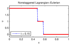
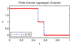
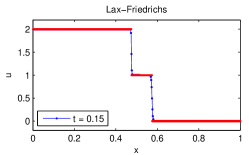
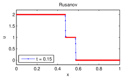
Figure 3: Numerical solutions to problem P1 at time $t=0.15$ (before shock).

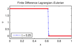
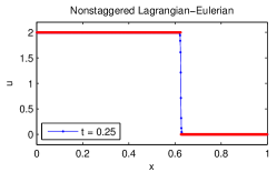
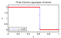
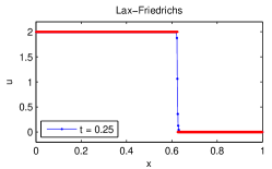
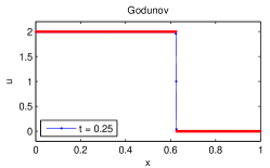
Figure 4: Numerical solutions to problem P1 at time $t=0.25$ (after shock).

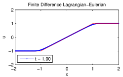
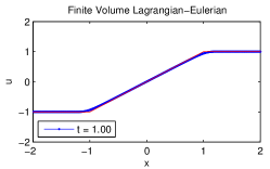
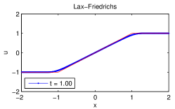
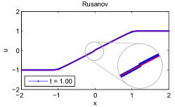
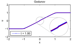
Figure 5: Numerical solutions to problem P2 at time $t=0.5$ (rarefaction). Notice that the Lagrangian-Eulerian scheme does not produce the well-known spurious glitch effect in the sonic rarefaction present in Godunov and Rusanov’s simulations.

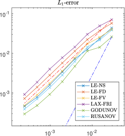
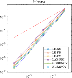
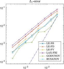
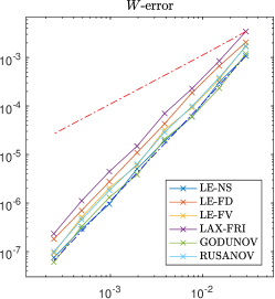
Figure 6: Log-log plots for norms $L^{1}$ and $W$ of the error versus the cell sizes for problem P1 at time $t=0.15$ (before shock; first two pictures) and at time $t=0.25$ (after shock; last two pictures). The top solid line represents the convergence of the Lax–Friedrichs numerical scheme, while the bottom solid line marks the convergence of the Godunov method. The error obtained with the Nonstaggered Lagrangian–Eulerian scheme in these cases approaches that of Godunov and is sometimes lower than that of Rusanov.

4.2 A nonlocal traffic model

We present numerical approximations of the classical Lighthill–Whitham–Richards (LWR) model for vehicular traffic [8], which consists of a continuity equation

$$\partial_{t}\rho+\partial_{x}\left(\rho V\right)=0,\qquad\rho\in[0,1],$$ (4.2)

where $\rho$ is the (average) vehicular density. Density $\rho$ is a function of $t$ (time), and $x$ is a position along a road with neither entries nor exits. In this equation, a speed law function $V=V(\rho)$ is defined as follows:

$$V(\rho)=V_{\max}(1-\rho)(1-\rho\ast\eta).$$ (4.3)

By setting $V_{\max}>0$, this flux function can be used as an LWR-type macroscopic model for vehicular traffic, where drivers adjust their speed according to the local traffic density. The convolution is realized with $\eta$ ($\alpha$ is chosen so that $\int_{\mathbb{R}}\eta=1$), which is defined as

$$\eta(x)=\begin{cases}\alpha\left((x_{1}-x)(x-x_{2})\right)^{5/2},\quad-x_{1}\leq x\leq x_{2}\\ 0,\quad\text{ otherwise.}\end{cases}$$ (4.4)

Parameters $x_{1}$ and $x_{2}$ are the horizon of each driver, in the sense that a driver situated at $x$ adjusts his speed according to the average vehicular density he sees on interval $[x-x_{1},x+x_{2}]$. We followed the exact same numerical approximation of the convolution integral presented in [8]. And we selected two situations (as in [8]): (1) the drivers look forward or (2) backward $(x_{1},x_{2})=(0,0.25)$ and $(x_{1},x_{2})=(0.25,0).$ The initial condition is given by

$$\rho_{0}(x)=\begin{cases}\frac{1}{2},\quad\quad-2.8\leq x\leq-1.8;\quad\quad\\ \frac{3}{4},\quad\quad-1.2\leq x\leq-0.2;\\ \frac{3}{4},\quad\quad 0.6\leq x\leq 1.0;\\ 1,\quad\quad 1.5\leq x<\infty;\\ 0,\quad\quad\text{ otherwise.}\end{cases}$$ (4.5)

which represents three groups of vehicles lining up in a queue. From [8], for any $\rho^{,}\in L^{1}(\mathbb{R};[0,1])$, the Cauchy problem with initial datum $\rho_{0}$ allows a unique solution $\rho=\rho(t,x)$, reaching values in $[0,1]$. The qualitative behaviors of the solution are rather different in the two situations in (4.3). The expected big oscillations in the vehicular density caused by the backward-looking case can be seen in Figure 8 (as opposed to the far more reasonable behavior in the forward-looking scenario in Figure 7). The structure of the numerical solutions presented here are in particularly good agreement with [8]. We will also present in Table 1 an error analysis, so that it is possible to observe that our method presents first-order accuracy behavior.

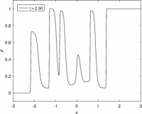
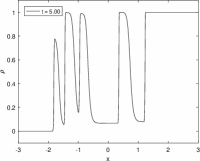
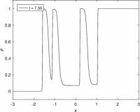
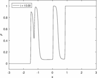
Figure 7: Backward horizon case with 2048 mesh points at times t = 2.50, 5.01, 7.50, 10.00. The shock heights and velocities agree with the results provided in [8]. In Figure 9, we can see a first-order behavior of accuracy in the numerical solutions.

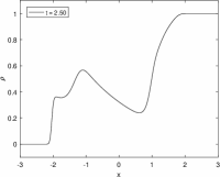
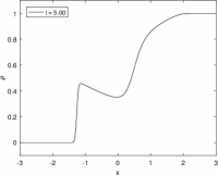
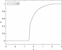
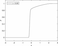
Figure 8: Forward horizon case with 512 mesh points at times t = 2.50, 5.01, 7.50, 10.00. The expected difference in the two solutions due to the position of the support of $\eta$ was correctly captured by our method.

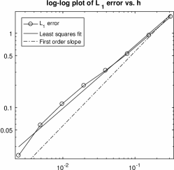
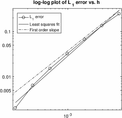
Figure 9: Log-log plots for norm $L^{1}$ of the error versus the cell sizes, for the traffic problem (4.3), at time $T=0.5$ with backward horizon (left) and problem 4.7 at time $T=0.5$ (right). We can see first-order behavior of accuracy in the numerical solutions.

Cells	$h$	$\|u-U\|_{L_{h}^{1}}$
$64$	$0.15625$	$9.4\times 10^{-1}$
$128$	$0.07813$	$5.29\times 10^{-1}$
$256$	$0.03906$	$3.17\times 10^{-1}$
$512$	$0.01953$	$1.99\times 10^{-1}$
$1024$	$0.00976$	$1.12\times 10^{-1}$
$2048$	$0.00488$	$5.82\times 10^{-2}$
$4096$	$0.00244$	$2.28\times 10^{-2}$
LSF $E(h)$		$5.034\times h^{0.856}$

Cells	$h$	$\|u-U\|_{L_{h}^{1}}$
$512$	$3.90\times 10^{-3}$	$2.46\times 10^{-1}$
$1024$	$1.95\times 10^{-3}$	$1.34\times 10^{-1}$
$2048$	$9.76\times 10^{-4}$	$6.68\times 10^{-2}$
$4096$	$4.88\times 10^{-4}$	$3.21\times 10^{-2}$
$8192$	$2.44\times 10^{-4}$	$1.52\times 10^{-2}$
$16384$	$1.22\times 10^{-4}$	$6.4\times 10^{-3}$
$32768$	$6.10\times 10^{-5}$	$2.04\times 10^{-3}$
LSF $E(h)$		$71.161\times h^{1.13037}$

Table 1: Left: Corresponding errors between the numerical approximations ($U$) and a reference solution ($u$) with 8192 mesh points for the nonlocal problem. Right: Corresponding errors between the numerical approximations ($U$) and a reference solution ($u$) for the variable $u_{1}$ with 65536 mesh points for the Keyfitz-Kranzer system problem. The bottom row in both tables presents least square fits for the error profiles.

4.3 The $2\times 2$ symmetric Keyfitz–Kranzer system

We consider the Cauchy problem for the $2\times 2$ Keyfitz–Kranzer system as in [24],

$$\begin{cases}u_{t}+(u\phi(|u|))_{x}=0,&\quad(x,t)\in\mathbb{R}\times(0,T),\\ u(x,0)=u_{0}(x),&\quad x\in\mathbb{R},\end{cases}$$ (4.6)

where $T>0$ is the final simulation time, $u$ is the unknown solution, such that $u=(u_{1},u_{2}):\mathbb{R}\times(0,T)\mapsto\mathbb{R}^{n}$ with $|u|:=\sqrt{u_{1}^{2}+u_{2}^{2}}$. The initial datum is given by $u_{0}=(u_{1}^{0},u_{2}^{0})\in L^{\infty}(\mathbb{R},\mathbb{R}^{n})$ and $\phi(r)$ is a scalar function such that $\phi(r)\in C^{1}(\mathbb{R}^{+})$, where $r\phi(r)\to 0$ as $r\to 0$. This system is a prototype of a non strictly hyperbolic system of conservation laws, serving as a model for the elastic string (see [20]). Nevertheless, such model appears in magnetohydrodynamics, where it has been used, for example, to explain certain features of the solar wind, such as in [9]. We can rewrite Eq. (4.6) in a more explicit form by introducing variable $r=|u|$ to approximate its strong generalized entropy solution (as in [24]):

$$\begin{cases}r_{t}+(r\phi(r))_{x}=0,&\quad(x,t)\in\mathbb{R}\times(0,T),\\ u_{t}+(u\phi(r))_{x}=0,&\quad(x,t)\in\mathbb{R}\times(0,T),\\ u(x,0)=u_{0}(x),\;r(x,0)=r_{0}(x)=|u_{0}(x)|,&\quad x\in\mathbb{R}.\end{cases}$$ (4.7)

Here, $\phi(r)=r^{2}-4r+5.5$. This function has a minimum at $r=2$; hence, the ordering of the eigenvalues changes, a nonconvex flux function. We tested the method with the following initial data $r_{0}=\sin(\pi x)+1.5$, $v_{0}=(\sin(\pi x),\cos(\pi x))$,$x\in[-1,1]$ with periodic boundary conditions. The solution to the Riemann problem with left state $u_{L}$ and right state $u_{R}$ consists of left, right, and middle states separated by shocks, rarefaction waves, or contact discontinuities along which only $r$ changes and by contact discontinuities along which only $v=u/r$ changes. Figure 10 illustrates the precise structure of the solution, which is also in good agreement with [24].

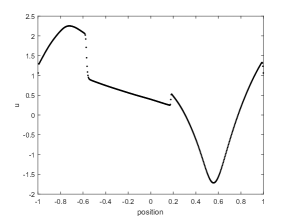
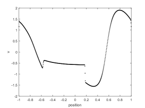
Figure 10: Symmetric Keyfitz–Kranzer system with 512 points at time t = 0.50, $u_{1}$ (left) and $u_{2}$ (right).

5 Concluding remarks

In this paper, we constructed a Lagrangian–Eulerian framework as a novel tool for balancing discretization in order to deal with nonlinear wave formations and rarefaction interactions in several applications. By implementing the weak asymptotic method, we used $L^{1}$-norm as well as a comparison between numerical studies and the W1 distance. As a result, we concluded that we were effectively computing the expected approximate solutions linked to problems exhibiting intricate nonlinear wave formations; for instance, Burgers’ equation (with initial data containing jumps that also exhibit non-linear rarefaction waves with sonic points and non-linear wave interaction in shock-wave focusing process in time-space), a nonlocal Lighthill-Whitham-Richards model for vehicular traffic model, and a $2\times 2$ symmetric Keyfitz–Kranzer system. The weak asymptotic solutions we computed with our novel Lagrangian–Eulerian framework have been shown to coincide with classical (regular) solutions and weak Kruzhkov entropy solutions. Our scheme is promising, and it has shown it is a suitable foundation to develop novel constructive methods in abstract as well as practical computational mathematics settings.

Appendix

Appendix A Proof that the reconstructions are Lipschitz continuous

In Section 3, to prove the convergence of our numerical scheme, we assumed that the reconstructions were Lipschitz continuous. The reconstructions were obtained from the slope limiters discussed in Section 2.4. Here, we prove, first, that each slope limiter (Eqs. $(\ref{mm2})$, $(\ref{mm3})$ and $(\ref{uno})$) is a Lipschitz function, and second, that the reconstruction for each case is also Lipschitz continuous.

The function $MM_{2}$ is Lipschitz continuous

Let $\vec{x}_{1}=(x_{1},y_{1})$ and $\vec{x}_{2}=(x_{2},y_{2})$, thus, from Eq. $(\ref{mm})$, we obtain

$$||\text{MM}_{2}(\vec{x}_{1})-\text{MM}_{2}(\vec{x}_{2})||=\left|{\frac{1}{2}\left[\text{sgn}(x_{1})+\text{sgn}(y_{1})\right]\min(|x_{1}|,|y_{1}|)-{\frac{1}{2}\left[\text{sgn}(x_{2})+\text{sgn}(y_{2})\right]\min(|x_{2}|,|y_{2}|)}}\right|.$$

We then divide our analysis into two possibilities:

(i) - First, we assume that $x_{1}\geq 0$, $y_{1}\geq 0$, $x_{2}\geq 0$ and $y_{2}\geq 0$ (the case in which all the negatives are similar). Thus $\frac{1}{2}\left[\text{sgn}(x_{1})+\text{sgn}(y_{1})\right]\min(|x_{1}|,|y_{1}|)=\hat{x}_{1}$, where $\hat{x}_{1}=x_{1}$ or $\hat{x}_{1}=y_{1}$, we also have that $\frac{1}{2}\left[\text{sgn}(x_{2})+\text{sgn}(y_{2})\right]\min(|x_{2}|,|y_{2}|)=\hat{x}_{2}$, where $\hat{x}_{2}=x_{2}$ or $\hat{x}_{2}=y_{2}$. Thus $||\text{MM}_{2}(\vec{x}_{1})-\text{MM}_{2}(\vec{x}_{2})||=|\hat{x}_{1}-\hat{x}_{2}|.$ Notice that, if $\hat{x}_{1}=x_{1}$ and $\hat{x}_{2}=x_{2}$, then $|\hat{x}_{1}-\hat{x}_{2}|=|x_{1}-x_{2}|$, and we have that

$$||\text{MM}_{2}(\vec{x}_{1})-\text{MM}_{2}(\vec{x}_{2})||=|\hat{x}_{1}-\hat{x}_{2}|=|x_{1}-x_{2}|\leq|x_{1}-x_{2}|+|y_{1}-y_{2}|=\left\lVert\vec{x}_{1}-\vec{x}_{2}\right\rVert.$$

On the other hand, if $\hat{x}_{1}=y_{1}$ and $\hat{x}_{2}=x_{2}$, then $|\hat{x}_{1}-\hat{x}_{2}|=|y_{1}-x_{2}|$. In this case, we have that $x_{1}>y_{1}$. If $y_{1}>x_{2}$, then we have that $|y_{1}-x_{2}|=y_{1}-x_{2}<x_{1}-x_{2}=|x_{1}-x_{2}|\leq|x_{1}-x_{2}|+|y_{1}-y_{2}|$. If $y_{2}>x_{2}>y_{1}$, then $|y_{1}-x_{2}|=x_{2}-y_{1}<y_{2}-y_{1}=|y_{1}-y_{2}|\leq|x_{1}-x_{2}|+|y_{1}-y_{2}|$, thus $||\text{MM}_{2}(\vec{x}_{1})-\text{MM}_{2}(\vec{x}_{2})||=|\hat{x}_{1}-\hat{x}_{2}|=\leq|x_{1}-x_{2}|+|y_{1}-y_{2}|=\left\lVert\vec{x}_{1}-\vec{x}_{2}\right\rVert.$ The case in which $\hat{x}_{1}=y_{1}$, $\hat{x}_{2}=y_{2}$, $\hat{x}_{1}=x_{1}$, and $\hat{x}_{2}=y_{2}$ is analogous to the previous one.

(ii) - Now, we assume that $x_{1}>0$, $y_{1}<0$, $x_{2}>0$, and $y_{2}>0$ (the other cases for which we have one pair with different signals and another pair with equal signals are similar to this case). Notice that, $\text{MM}_{2}(\vec{x}_{1})=0$, thus $||\text{MM}_{2}(\vec{x}_{1})-\text{MM}_{2}(\vec{x}_{2})||=|\hat{x}_{2}|=\hat{x}_{2},$ where $\hat{x}_{2}=x_{2}$ or $\hat{x}_{2}=y_{2}$. If $\hat{x}_{2}=x_{2}$, then we have that $\hat{x}_{2}=x_{2}<x_{2}-y_{1}<y_{2}-y_{1}\leq|x_{2}-x_{1}|+|y_{2}-y_{1}|$, where $x_{2}<x_{2}-y_{1}$ because $y_{1}$ is negative. On the other hand, if $\hat{x}_{2}=y_{2}$, then we have that $\hat{x}_{2}=y_{2}<y_{2}-y_{1}\leq|x_{2}-x_{1}|+|y_{2}-y_{1}|$. In any case $||\text{MM}_{2}(\vec{x}_{1})-\text{MM}_{2}(\vec{x}_{2})||=|\hat{x}_{2}|=\hat{x}_{2}<||\vec{x}_{1}-\vec{x}_{2}||.$ Then, the function $\text{MM}_{2}$ is Lipschitz continuous and its Lipschitz constant equals 1.

The function $\text{MM}_{3}$ is Lipschitz continuous

Let $\vec{x}_{1}=(x_{1},y_{1},z_{1})$, $\vec{x}_{2}=(x_{2},y_{2},z_{2})$ and $\text{MM}_{2}(x,y)$ be Lipschitz continuous with a constant equal to 1

$$\left\lVert\text{MM}_{3}(\vec{x}_{1})-\text{MM}_{3}(\vec{x}_{2})\right\rVert=\left\lVert\text{MM}_{2}\left(\text{MM}_{2}(x_{1},y_{1}),z_{1}\right)-\text{MM}_{2}\left(\text{MM}_{2}(x_{2},y_{2}),z_{2}\right)\right\rVert$$

$$\leq|\text{MM}_{2}(x_{1},y_{1})-\text{MM}_{2}(x_{2},y_{2})|+|z_{1}-z_{2}|\leq|x_{1}-x_{2}|+|y_{1}-y_{2}|+|z_{1}-z_{2}|=\left\lVert\vec{x}_{1}-\vec{x}_{2}\right\rVert.$$ (A.1)

From inequality $(\ref{ettbs})$, we prove that $\text{MM}_{3}$ is Lipschitz continuous with a constant equal to 1.

The functions measuring variations are Lipschitz continuous

The function $U^{\prime}_{j}$ that measures variations is defined in Eqs. $(\ref{mm2})$, $(\ref{mm3})$, and $(\ref{uno})$.

For Eq. $(\ref{mm2})$, we defined $U^{\prime}_{j}=\text{MM}_{2}\left(F_{1}(u_{j+1},u_{j},u_{j-1})\right),$ where $F_{1}(x,y,z)=(x-y,y-z)$. If we prove that $F_{2}(x,y,z)$ is a Lipschitz function, then, since $U^{\prime}_{j}$ is a composition of two Lipschitz continuous, $U^{\prime}$ is also Lipschitz continuous. Let $\vec{x}_{1}=(x_{1},y_{1},z_{1})$ and $\vec{x}_{2}=(x_{2},y_{2},z_{2})$, thus

$$\left\lVert F_{1}(\vec{x}_{1})-F_{1}(\vec{x}_{2})\right\rVert =\left\lVert(x_{1}-x_{2}-(y_{1}-y_{2}),y_{1}-y_{2}-(z_{1}-z_{2}))\right\rVert$$

$$\leq|x_{1}-x_{2}|+2|y_{1}-y_{2}|+|z_{1}-z_{2}|\leq 2\left\lVert\vec{x}_{1}-\vec{x}_{2}\right\rVert.$$

For Eq. $(\ref{mm3})$, we defined $U^{\prime}_{j}=\text{MM}_{3}\left(F_{2}(u_{j-1},u_{j},u_{j+1})\right),$ where $F_{2}(x,y,z)=(\alpha(x-y),x-z,\alpha(y-z))$ and $\alpha$ is a nonnegative number. We have now proven that $F_{2}$ is a Lipschitz function, thus $U^{\prime}_{j}$ is also Lipschitz continuous. Let $\vec{x}_{1}=(x_{1},y_{1},z_{1})$ and $\vec{x}_{2}=(x_{2},y_{2},z_{2})$, thus

$$\left\lVert F_{2}(\vec{x}_{1})-F_{2}(\vec{x}_{2})\right\rVert =\left\lVert\left(\alpha(x_{1}-x_{2}-(y_{1}-y_{2})),x_{1}-x_{2}-(z_{1}-z_{2}),\alpha(y_{1}-y_{2}-(z_{1}-z_{2}))\right)\right\rVert$$

$$\leq\alpha|x_{1}-x_{2}|+\alpha|y_{1}-y_{2}|+|x_{1}-x_{2}|+|z_{1}-z_{2}|+\alpha|y_{1}-y_{2}|+\alpha|z_{1}-z_{2}|$$

$$\leq(\alpha+1)|x_{1}-x_{2}|+2\alpha|y_{1}-y_{2}|+(\alpha+1)|z_{1}-z_{2}|\leq(\alpha+2)\left\lVert\vec{x}_{1}-\vec{x}_{2}\right\rVert.$$

For Eq. $(\ref{uno})$, we defined $U^{\prime}_{j}=\text{MM}_{2}\left(H(u_{j+2},u_{j+1},u_{j},u_{j-1},u_{j-2})\right).$ Here, $H$ is a more complex function we defined from other auxiliary functions. We defined

$$F_{3}(x,y,z,w)=(x-2y+z,y-2z+w)\quad\text{ and }\quad F_{4}(x,y,z,w)=\frac{1}{2}\text{MM}_{2}(F_{3}(x,y,z,w)).$$

Using similar calculations, we can prove that $F_{3}(x,y,z,w)$ is a Lipschitz function. Since $F_{4}(x,y,z,w)$ is a composition of Lipschitz function, it is also a Lipschitz function. Notice that the function $\delta^{2}$ that appears in Eq. $(\ref{uno})$ can be written as $\delta^{2}(u_{j+2},u_{j+1},u_{j},u_{j-1})=F_{4}(u_{j+2},u_{j+1},u_{j},u_{j-1}).$ We defined function $H(x,y,z,w,u)$ as $H(x,y,z,w,u)=(y-z-F_{4}(x,y,z,w),z-w+F(y,z,w,u)).$ Notice that $H(x,y,z,w,u)$ is obtained as a sum of Lipschitz function; thus, it is Lipschitz as well.

Remark A.1.

Since the reconstructions were obtained from linear combinations of slope limiters and function measuring variations, these reconstructions are also Lipschitz continuous.

Appendix B The extension of derivatives of $f^{+}$ and $f^{-}$

Sometimes, we are interested in using results for which a continuous derivative of $f^{+}$ and $f^{-}$ is necessary. Since these functions are well defined, and their derivative is not well defined only on some points for which $f$ changes their signal, then we can extend the derivative of $f^{+}$ and $f^{-}$ in a continuous (but not smooth) way. First, we assume that $f(x)$ has only a finite number of zeros for which $f$ changes their signal (we are disregarding the zeros for which $f$ does not change their signal); for instance, we denote these zeros as $x_{0}<x_{1}\cdots<x_{n}$. For the sake of simplicity, we assume that $n=2k$ for some $k\in\mathbb{N})$ (if $n=2k+1$, we use a similar argument).

We assume that $f$ satisfies

$$f(x)=\begin{cases}f(x)>0,&\text{ if }x\in(-\infty,x_{0})\\ f(x)<0,&\text{if }x\in(x_{0},x_{1})\\ \vdots\\ f(x)>0,&\text{ if }x\in(x_{n-1},x_{n})\\ f(x)<0,&\text{if }x\in(x_{n},\infty)\\ f(x)=0,&\text{if }x=\{x_{0},\cdots,x_{n}\}\end{cases}\Rightarrow f(x)=\begin{cases}f(x)>0,&\text{ if }x\in(-\infty,x_{0})\bigcup\left[\bigcup\limits_{i=0}^{N/2-1}(x_{2i+1},x_{2i+2})\right]\\ f(x)=0,&\text{if }x=\{x_{0},\cdots,x_{n}\}\\ f(x)<0,&\text{ if }x\in\left[\bigcup\limits_{i=0}^{N/2-1}(x_{2i},x_{2i+1})\right]\bigcup(x_{n},\infty)\end{cases}$$

The derivatives of $f^{+}$ and $f^{-}$ are not defined in $x_{i}$ for $i=0,\cdots,n$. To obtain a continuous extension, we define the derivative of $f^{+}$, denoted as $(\hat{f}^{+})^{\prime}$, as

$$(\hat{f}^{+})^{\prime}=\begin{cases}f^{\prime}(x),&\text{ if }x\in(-\infty,x_{0})\bigcup\left[\bigcup\limits_{i=0}^{N/2-1}(x_{2i+1},x_{2i+2})\right].\\ f^{\prime}(x_{2i})\left(\frac{x_{2i}+\delta-x}{\delta}\right),&\text{ if }x\in\left[\bigcup\limits_{i=0}^{N/2-1}[x_{2i},x_{2i}+\delta]\right]\bigcup[x_{n},x_{n}+\delta].\\ f^{\prime}(x_{2i+1})\left(\frac{x-x_{2i+1}+\delta}{\delta}\right),&\text{ if }x\in\bigcup\limits_{i=0}^{N/2-1}(x_{2i+1}-\delta,x_{2i+1}).\\ 0,&\text{ if }x\in\left[\bigcup\limits_{i=0}^{N/2-1}(x_{2i}+\delta,x_{2i+1}-\delta]\right]\bigcup(x_{n}+\delta,\infty).\end{cases}$$ (B.1)

In Eq. $(\ref{fdefinem})$, $\delta$ is arbitrary. For instance, we can take $\delta$, thus satisfying $\delta=\min_{i=\{0,\cdots,n-1\}}\left(\frac{x_{i+1}-x_{i}}{3}\right).$ Using $f=f^{+}-f^{-}$ and therefore $f^{-}=f^{+}-f$, we propose a continuous extension for the derivative of $f^{-}$, denoted as $(\hat{f}^{-})^{\prime}$, as $(\hat{f}^{-})^{\prime}=(\hat{f}^{+})^{\prime}-f^{\prime}.$

Appendix C The pre-compactness of sequence $u(x,t,\epsilon)$

To prove that the sequence $u(x,t,\epsilon)$ is pre-compact, we used the results in another paper [2]. The first result we need is Lemma 1 in [2]:

Lemma 1. Suppose that $u(x)\in L^{1}(\mathbb{T}^{n})$, $h>0$. Then

$$\int_{\mathbb{T}^{n}}|u(x)(\text{sgn}u)^{h}(x)-|u(x)||dx\leq 2\omega^{x}(h),$$

where $\omega^{x}(h)=\sup_{|\Delta x|\leq h}\int_{\mathbb{T}^{n}}|u(x+\Delta x)-u(x)|dx,$ is the continuity modulus of $u(x)$ in $L^{1}(\mathbb{T}^{n})$.

Here, $\mathbb{T}^{n}$ is the $n$-dimensional torus. In this study, we are interested in a one-dimensional problem. For $n=1$, $\mathbb{T}^{n}$ reduces to ${\mathbb{S}^{1}}$. Since the proof of the previous Lemma does not depend on the scheme, we refer to [2]. Notice that $\omega^{x}(h)$ is a measure of TVNI_$\epsilon$, as described in Eq. $(\ref{tv})$. Thus, under the same hypothesis of Proposition 3.5, we can prove the following Corollary:

Corollary C.1.

Let us assume that $u(x,t,\epsilon)$ is given by scheme $(\ref{ODE})$ and satisfies the hypothesis of Proposition 3.5. Then, for all $t>0$, $\Delta x\in\mathbb{R}$, we have that

$$\int_{\mathbb{S}^{1}}|u(x+\Delta x,t,\epsilon)-u(x,t,\epsilon)|dx\leq\int_{\mathbb{S}^{1}}|u_{0}(x+\Delta x,t,\epsilon)-u_{0}(x,t,\epsilon)|\leq\omega^{x}(|\Delta x|),$$

where $\omega^{x}(|\Delta x|)\leq\sup_{|\Delta x|\leq h}\int_{\mathbb{S}^{1}}|u_{0}(x+\Delta x,t,\epsilon)-u_{0}(x,t,\epsilon)|$ is the continuity modulus of the initial data $u_{0}(x)$ in ${\mathbb{S}^{1}}$.

The proof of Corollary C.1 follows from Proposition 3.5. Now, we prove the result to obtain the pre-compactness of sequence $u(x,t,\epsilon)$. The first useful result, similar to that obtained in [2], is

Lemma C.2.

Let us assume that $\phi(x)\in C^{1}({\mathbb{S}^{1}})$. Then $\forall\Delta t>0$,

$$\int_{\mathbb{S}^{1}}(u(c,t+\Delta t,\epsilon)-u(x,t,\epsilon)\phi(x)dx\leq N||\nabla\phi||_{\infty}\Delta t\mu(\mathbb{S}^{1}).$$ (C.1)

Here, $\mu(\mathbb{S}^{1})$ is the measure of $\mathbb{S}^{1}$ and $N=\max_{|u|\leq\bar{M}}(|u|(|f^{+}(\hat{u})|+|f^{-}(\hat{u})|)\quad\text{ and }\quad\bar{M}=||u_{0}||_{\infty}.$

Proof. Let us denote $I(t)=\int_{{\mathbb{S}^{1}}}u(x,t,\epsilon)\phi(x)$. Differentiating $I(t)$ from $t$ and using $(\ref{ODE})$, we have that

$$I^{\prime}(t) =\frac{1}{\epsilon}\int_{{\mathbb{S}^{1}}}\left(u_{{}_{\epsilon-1}}f^{+}\left(\hat{u}_{{}_{\epsilon-1/2}}\right)-u_{{}_{\epsilon}}f^{+}\left(\hat{u}_{{}_{\epsilon+1/2}}\right)-u_{{}_{\epsilon}}f^{-}\left(\hat{u}_{{}_{\epsilon-1/2}}\right)+u_{{}_{\epsilon+1}}f^{-}\left(\hat{u}_{{}_{\epsilon+1/2}}\right)\right)\phi(x)dx$$

$$=\int_{{\mathbb{S}^{1}}}u_{{}_{\epsilon}}f^{+}\left(\hat{u}_{{}_{\epsilon+1/2}}\right)\frac{\phi(x+\epsilon)-\phi(x)}{\epsilon}dx-\int_{{\mathbb{S}^{1}}}u_{{}_{\epsilon}}f^{-}\left(\hat{u}_{{}_{\epsilon+1/2}}\right)\frac{\phi(x+\epsilon)-\phi(x)}{\epsilon}dx.$$ (C.2)

Since $I^{\prime}(t)=G(t)$ implies that $|I(t+\Delta t)-I(t)|\leq\max G(t)\Delta t$, we can estimate RHS of Eq. $(\ref{eqt})$ as

$$|RHS|\leq\int_{{\mathbb{S}^{1}}}|u_{{}_{\epsilon}}||f^{+}\left(\hat{u}_{{}_{\epsilon+1/2}}\right)|\left|\frac{\phi(x+\epsilon)-\phi(x)}{\epsilon}\right|dx+\int_{{\mathbb{S}^{1}}}|u_{{}_{\epsilon}}||f^{-}\left(\hat{u}_{{}_{\epsilon+1/2}}\right)|\left|\frac{\phi(x+\epsilon)-\phi(x)}{\epsilon}\right|dx.$$

Using $\left|\frac{\phi(x\pm\epsilon)-\phi(x)}{\epsilon}\right|dx\leq||\nabla\phi||_{\infty}$ and $|u(x,t,\epsilon)|\leq\bar{M}$, Eq. $(\ref{dtt})$. follows $\quad\quad\square$

Since we obtained similar estimates in [2], we used Lemma 3 in reference [2].

Lemma 3. For every $t\geq 0$, $\Delta t>0$

$$\int_{{\mathbb{S}^{1}}}|u(x,t+\Delta t,\epsilon)-u(x,t,\epsilon)|dx\leq\omega^{t}(\Delta t),$$

where $\omega^{t}(\Delta t)=\inf_{h>0}(4\omega^{x}(h)+cN\Delta t/h)$, and $c$ is a universal constant.

Note that, in $\omega^{t}(\Delta t)$, since this parameter is the infimum, $\omega^{t}(\Delta t)$ for fixed $\Delta t$ reduces to $\inf_{h>0}(4\omega^{x}(h))$.

Moreover, since $\omega^{x}(h)\longrightarrow 0$ as $h\longrightarrow 0$ and does not depend on $\epsilon$ (based on previous results), family $u(x,t,\epsilon)$ is uniformly bounded and equicontinuous in $L^{1}({\mathbb{S}^{1}}\times[0,T])$ for every $T>0$. Thus, $u(x,t,\epsilon)$ is a pre-compact sequence in $L^{1}({\mathbb{S}^{1}}\times[0,T])$, which implies that we can extract a sequence $\epsilon_{k}\longrightarrow 0$ such that $u_{k}(x,t)=u(x,t,\epsilon_{k})\longrightarrow u(x,t)$ as $k\longrightarrow\infty$ in $L_{loc}^{1}({\mathbb{S}^{1}}\times[0,\infty])$.

References

- [1]
- [2] Abreu, E., Colombeau, M., Panov, E.: Weak asymptotic methods for scalar equations and systems. Journal of mathematical analysis and applications 444(2), 1203–1232 (2016)
- [3] Abreu, E., Colombeau, M., Panov, E.Y.: Approximation of entropy solutions to degenerate nonlinear parabolic equations. Zeits. für angew. Mathem. und Phys. 68(6), 133 (2017)
- [4] Abreu, E., Lambert, W., Pérez, J., Santo, A.: A new finite volume approach for transport models and related applications with balancing source terms. Math. and Comp. in Sim. 137, 2–28 (2017)
- [5] Abreu, E., Lambert, W., Pérez, J., Santo, A.: A weak asymptotic solution analysis for a Lagrangian–Eulerian scheme for scalar hyperbolic conservation laws. Proceedings of the 17-th Conference on Hyperbolic Problems Theory, Numerics, Applications, , June 25-29, 2018 University Park, Pennsylvania, USA. 1 (2020)
- [6] Abreu, E., Matos, V., Perez, J., Rodriguez-Bermudez, P.: A class of Lagrangian–Eulerian shock-capturing schemes for first-order hyperbolic problems with forcing terms. Journal of Scientific Computing 86(1), 1–47 (2021)
- [7] Abreu, E., Pérez, J.: A fast, robust, and simple Lagrangian–Eulerian solver for balance laws and applications. Computers & Mathematics with Applications 77(9), 2310–2336 (2019)
- [8] Amorim, P., Colombo, R.M., Teixeira, A.: On the numerical integration of scalar nonlocal conservation laws. ESAIM: Math. Model. and Numerical Analysis 49(1), 19–37 (2015)
- [9] Cohen, R.H., Kulsrud, R.M.: Nonlinear evolution of parallel-propagating hydromagnetic waves. The Physics of Fluids 17(12), 2215–2225 (1974)
- [10] Colombeau, M.: Limits of nonlinear weak asymptotic methods. Journal of Mathematical Analysis and Applications 395(2), 587–595 (2012)
- [11] Colombeau, M.: A consistent numerical scheme for self-gravitating fluid dynamics. Numerical Methods for Partial Differential Equations 29(1), 79–101 (2013)
- [12] Danilov, V., Mitrovic, D.: Delta shock wave formation in the case of triangular hyperbolic system of conservation laws. Journal of Differential Equations 245(12), 3704–3734 (2008)
- [13] Danilov, V., Omel’Yanov, G., Shelkovich, V.: Weak asymptotics method and interaction of nonlinear waves. Translations of the American Mathematical Society-Series 2 208, 33–164 (2003)
- [14] Danilov, V., Shelkovich, V.: Delta-shock wave type solution of hyperbolic systems of conservation laws. Quarterly of Applied Mathematics 63(3), 401–427 (2005)
- [15] Danilov, V., Shelkovich, V.: Dynamics of propagation and interaction of -shock waves in conservation law systems. Journal of Differential Equations 211(2), 333–381 (2005)
- [16] Douglas, J., Pereira, F., Yeh, L.M.: A locally conservative eulerian–lagrangian numerical method and its application to nonlinear transport in porous media. Computational Geosciences 4(1), 1–40 (2000)
- [17] Fjordholm, U.S., Solem, S.: Second-order convergence of monotone schemes for conservation laws. SIAM Journal on Numerical Analysis 54(3), 1920–1945 (2016)
- [18] Godlewski, E., Raviart, P.A.: Entropy stable schemes. In: Hyperbolic systems of conservation laws, vol. 3,4, p. 252. Mathématiques and Applications, Elipses (1991)
- [19] Harten, A.: High resolution schemes for hyperbolic conservation laws. Journal of computational physics 135(2), 260–278 (1997)
- [20] Keyfitz, B.L., Kranzer, H.C.: A system of non-strictly hyperbolic conservation laws arising in elasticity theory. Archive for Rational Mechanics and Analysis 72(3), 219–241 (1980)
- [21] Nilsson, B., Shelkovich, V.: Mass, momentum and energy conservation laws in zero-pressure gas dynamics and delta-shocks. Applicable Analysis 90(11), 1677–1689 (2011)
- [22] Omel’yanov, G.A., Segundo-Caballero, I.: Asymptotic and numerical description of the kink/antikink interaction. Elect. Jour. of Dif. Equat. (EJDE)[electronic only] 2010, Paper–No (2010)
- [23] Panov, E.Y., Shelkovich, V.: ’-shock waves as a new type of solutions to systems of conservation laws. Journal of Differential Equations 228(1), 49–86 (2006)
- [24] Risebro, N.H., Weber, F.: A note on front tracking for the Keyfitz–Kranzer system. Journal of Mathematical Analysis and Applications 407(2), 190–199 (2013)
- [25] Shelkovich, V.: The Riemann problem admitting -, ’-shocks, and vacuum states (the vanishing viscosity approach). Journal of Differential Equations 231(2), 459–500 (2006)