Multi-sample estimation of centered log-ratio matrix in microbiome studies

Abstract

In microbiome studies, one of the ways of studying bacterial abundances is to estimate bacterial composition based on the sequencing read counts. Various transformations are then applied to such compositional data for downstream statistical analysis, among which the centered log-ratio (clr) transformation is most commonly used. Due to limited sequencing depth and DNA dropouts, many rare bacterial taxa might not be captured in the final sequencing reads, which results in many zero counts. Naive composition estimation using count normalization leads to many zero proportions, which makes clr transformation infeasible. This paper proposes a multi-sample approach to estimation of the clr matrix directly in order to borrow information across samples and across species. Empirical results from real datasets suggest that the clr matrix over multiple samples is approximately low rank, which motivates a regularized maximum likelihood estimation with a nuclear norm penalty. An efficient optimization algorithm using the generalized accelerated proximal gradient is developed. Theoretical upper bounds of the estimation errors and of its corresponding singular subspace errors are established. Simulation studies demonstrate that the proposed estimator outperforms the naive estimators. The method is analyzed on Gut Microbiome dataset and the American Gut project.

1 Introduction

Recent studies have demonstrated that the microbiome composition varies across individuals due to different health and environmental conditions [10, 8]. Microbiome is associated with many complex diseases such as obesity, atherosclerosis, and Crohn’s disease [35, 20, 24]. With the development of next-generation sequencing technologies, the human microbiome can be quantified by using direct DNA sequencing of either marker genes or the whole metagenomes. After aligning the sequence reads to the reference microbial genomes, one obtains counts of sequencing reads that can be assigned to a set of bacterial taxa observed in the samples. Such count data provide information about the relative abundance of different bacteria in different samples.

Due to limited sequencing depths and DNA dropouts during sequencing, count results many zeros and therefore the relative proportional of bacterial taxa often include many zeros. Excessive zeros in the proportions complicate many downstream data analyses. Since the pioneering work of [1, 2, 14], several techniques have been proposed to deal with zeros in compositional or count data (see [27] for an overview). When the data are compositional, they need to be scaled so that subsequent analysis are scale-invariant, and geometrically this means to force them into the open simplex. A common practice to analyze compositional data is to map bijectively the compositions into the ordinary Euclidean space through a suitable transformation, so that standard multivariate analysis techniques can be used [2, 14]. Among many such transformations [2, 14, 3], the center log-ratio (clr) tranformation, defined as the logarithms of the bacterial composition subtracted by logarithm of the geometric mean, is most widely used in practical analysis of microbiome data. After such transformation, one can then apply the standard statistical analysis methods such as the principal component analysis based on the clr transformed data [2, 16].

Since the original data observed are counts instead of compositions in microbiome studies, one has to first estimate the compositions before applying the clr transformation. The most commonly applied methods in composition data analysis involve a two-step procedure. One first estimates the composition using the observed count data and then performs the clr transformation [26, 8]. Since the counts often includes many zeros, such zeros can just be replaced by an arbitrarily small numbers so that one can furtherly apply the clr transformation. One drawback of estimating the clr matrix from the estimated compositions is that the uncertainty in the estimated compositions is not accounted when they are transformed using the clrs.

In this paper, we propose a method to estimate the clr matrix directly based on the observed count data. One key idea of the proposed method is to estimate the clr matrix of compositions of mutiple samples together, i.e., the clr matrix estimated from the count data from multiple samples. This effectively borrows information across multiple samples in order to obtain better estimate of the clr for each of the samples. More specifically, our proposed approach is based on a penalized likelihood estimation parameterized directly based on the clr matrix, where a nuclear norm penalty on the clr matrix is imposed to capture the expected approximate low-rank structure of the clr matrix. The low rank assumption is based on the empirical observations that the bacteria taxa abundances tend to be highly correlated and individual gut microbiome samples tend to cluster together to form discrete microbial communities. This is different from the approach of [8], where the low-rank assumption is directly imposed on the compositional matrix. Since there is no constraints on the clr matrix (except trivial constraints that sum of each rows to be zero), we develop a generalized accelerated proximal gradient algorithm to efficiently perform the optimization. The computation is faster than that of [8] where a simplex projection step is needed to account for the bounded simplex constraints.

We obtain the estimation bounds of the proposed estimator and its corresponding singular vector under both the exact low-rank and approximate low-rank settings. We present simulation results to compare our estimate and commonly used zero-replacement estimate. Finally, we demonstrate the methods using the data set from [38] and data set from the American Gut Project [29].

2 A Poisson-Multinomial Model for Microbiome Count Data

We refer to any $u\in\mathbb{R}^{p}$ as a composition vector if $u_{i}>0$ for $i=1,2,\ldots,p$ and $\displaystyle\sum_{i=1}^{p}u_{i}=1$. The data observed in typical marker gene-based microbiome studies (i.e., 16S rRNA marker gene) can be summarized as follows. Let $N_{i}$ be the total number of sequencing reads for the $i$th sample that can be assigned to one of the $p$ bacterial taxa, and $W_{ij}$ be the read count that can be assigned to the $j$th taxon for $j=1,\cdots,p$, where $\displaystyle N_{i}=\sum_{j=1}^{p}W_{ij}$. It is natural to model the count data ${\mathbf{W}}_{i}=(W_{ij},j=1,\cdots,p)$ using a multinomial distribution with composition parameter ${\mathbf{X}}_{i}^{*}=(X_{ij},j=1,\cdots,p)$ with $\displaystyle\sum_{j=1}^{p}X_{ij}=1$ [8]. Let ${\mathbf{X}}^{*}=({\mathbf{X}}^{*}_{ij})\in\mathbb{R}^{n\times p}$ denote the $n\times p$ compositional matrix.

Since each row of the compositional matrix ${\mathbf{X}}$ (${\mathbf{X}}$ can be true parameter ${\mathbf{X}}^{*}$ or estimated one $\hat{{\mathbf{X}}}$) is within the $p-1$ dimensional simplex with a unit sum constraint, certain transformation is often needed for downstream statistical analysis, including principal component analysis, estimation of covariance and regression analysis. One of the transformations that has been widely used in compositional data analysis is the clr transformation [2, 1], which is defined as $\mathbf{Z}_{ij}=\log(X_{ij}/g({\mathbf{X}}_{i}))$ where $g({\mathbf{a}})=\left(\prod_{i=1}^{p}a_{i}\right)^{1/p}$ is the geometric mean of the $p$ proportions. This can be written as a vector form as

$$\mathbf{Z}_{i}=\textsc{clr}({\mathbf{X}}_{i})=\log{\mathbf{X}}_{i}\cdot\left(\mathbf{I}_{p}-\frac{1}{p}{\bf 1}_{p}{\bf 1}_{p}\right).$$

The inverse of the clr transformation, which returns the original compositional vector ${\mathbf{X}}^{*}_{i}$, is actually the softmax function defined as

$${\mathbf{X}}_{i}=\textsc{clr}^{-1}(\mathbf{Z}_{i})={\text{softmax}}(\mathbf{Z}_{i})=\left(\frac{\exp\left(Z_{ij}\right)}{\sum_{k=1}^{p}\exp\left(Z_{ik}\right)}\right)_{n\times p},$$

and the gradient of the softmax function is

$$\nabla{\text{softmax}}(\mathbf{Z}_{i})={\rm diag}\left\{{\text{softmax}}(\mathbf{Z}_{i})\right\}-\left[{\text{softmax}}(\mathbf{Z}_{i})\right]^{T}{\text{softmax}}(\mathbf{Z}_{i})\in{\rm I\!R}^{p\times p}.$$

We let $\mathbf{Z}^{*}=(\mathbf{Z}^{*}_{ij})\in\mathbb{R}^{n\times p}$ denote the matrix of the underlying true centered log-ratio transformation of $n$ samples over $p$ taxa. Different from the work focusing on estimating ${\mathbf{X}}^{*}\in{\rm I\!R}^{n\times p}$ [8, 26], our goal is to estimate this clr matrix $\mathbf{Z}^{*}$ based on the observed counts ${\mathbf{W}}\in{\rm I\!R}^{n\times p}$.

Using the clr matrix $\mathbf{Z}^{*}$ as the parameter, the proposed Poisson-multinomial model for count-compositional data can be written as

$$N_{i} \sim \text{Pois}(\nu_{i}),i=1,2,\ldots,n;$$

$${\mathbf{P}}_{\mathbf{Z}_{i}^{*}}\left(W_{i1},\ldots,W_{ip}|N_{i}\right) = \frac{N_{i}!}{\prod_{j=1}^{p}W_{ij}!}\prod_{j=1}^{p}\left(X^{*}_{ij}\right)^{W_{ij}},i=1,2,\ldots,n.$$ (1)

where $X_{ij}^{*}={\text{softmax}}\left(\mathbf{Z}_{i}^{*}\right)_{j}=\textsc{clr}^{-1}\left(\mathbf{Z}_{i}^{*}\right)_{j}$.

The maximum likelihood estimation (of each composition vector in each row) provides one naive estimation $\hat{\mathbf{Z}}^{\rm MLE}$ of the clr matrix $\mathbf{Z}^{*}$, which is equivalent to estimating each row $\mathbf{Z}^{*}_{i}\in{\rm I\!R}^{1\times p}$ separately using only the data observed for the $i$th sample. However, $\hat{\mathbf{Z}}^{\rm MLE}$ cannot resolve zero-count issue: $\hat{Z}_{ij}^{\rm MLE}=-\infty$ and then ${\text{softmax}}\left(\hat{\mathbf{Z}}^{\rm MLE}_{i}\right)_{j}=0$ when $W_{ij}=0$. One standard and commonly used method of avoiding assigning zeros to $\hat{X}_{ij}$ is the zero-replacement estimation $\hat{{\mathbf{X}}}^{zr}$:

$$\hat{X}_{ij}^{\rm zr}=\frac{W_{ij}\wedge a}{\sum_{j=1}^{p}\left(W_{ij}\wedge a\right)},$$

where $a$ is an arbitrarily small number, but commonly set $a=0.5$ [7, 8, 2, 27, 28].

On the other hand, empirical observations in real microbiome data suggest that the clr matrix $\mathbf{Z}^{*}$ or composition matrix ${\mathbf{X}}^{*}$ is usually approximate low-rank due to dependency among the bacterial taxa. In this paper, we explore this low-rank structure $\mathbf{Z}^{*}$ to provide an improved estimate of $\mathbf{Z}^{*}$. This is different from [8], where composition matrix ${\mathbf{X}}^{*}$ is assumed to be approximate low-rank.

3 Regularized Estimation of the Centered-Log-Ratio Matrix and the Computational Algorithm

3.1 Regularized estimation of the centered-log-ratio matrix

In order to improve the estimate of the clr matrix $\mathbf{Z}^{*}$, the approximate low-rank structure of the $\mathbf{Z}^{*}$ is explored. The co-occurrence patterns [15], various symbiotic relationships in microbial communities [37, 18, 9] and samples in similar microbial communities are expected to lead to an approximately low-rank structure of the clr matrix in the sense that the singular values of $\mathbf{Z}^{*}$ decay to zero in a fast rate. Such a low-rank structure of $\mathbf{Z}^{*}$ is further investigated in our real data analysis in section 6, showing the empirical evidence of approximate low-rank clr matrix. We propose the following nuclear-norm penalized estimation of the clr matrix $\mathbf{Z}^{*}$ by exploring the low-rank structure of such a matrix,

$$\hat{\mathbf{Z}}(\lambda)\in\arg\min_{\mathbf{Z}{\bf 1}_{p}={\vec{\mathbf{0}}}_{n}}\mathcal{L}_{N}\left(\mathbf{Z};{\mathbf{W}}\right)+\lambda\left\|\mathbf{Z}\right\|_{*},$$ (2)

where

$$\mathcal{L}_{N}\left(\mathbf{Z};{\mathbf{W}}\right) \triangleq -\frac{1}{N}\sum_{i=1}^{n}N_{i}\mathcal{L}_{N_{i}}(\mathbf{Z}_{i};{\mathbf{W}})\triangleq-\frac{1}{N}\sum_{i=1}^{n}\sum_{j=1}^{p}W_{ij}\log\left\{{\text{softmax}}\left(\mathbf{Z}_{i}\right)_{j}\right\}$$

$$= -\frac{1}{N}\sum_{i=1}^{n}\sum_{j=1}^{p}W_{ij}\log\left(\frac{e^{z_{ij}}}{\sum_{j=1}^{p}e^{z_{ij}}}\right)=\frac{1}{N}\sum_{i=1}^{n}\left\{N_{i}\log\left(\sum_{j=1}^{p}e^{z_{ij}}\right)-\sum_{j=1}^{p}W_{ij}z_{ij}\right\}.$$

The proposed estimator (2) is a regularized nuclear norm minimization which can be solved by either semidefinite programming via interior-point semidefinite programming (SDP) solver, or first-order method via Templates for First-Order Conic Solvers (TFOCS). However the interior-point SDP solver computes the nuclear norm via a less efficient eigenvalue decomposition, which does not scale well with large $n$ and $p$. TFOCS on the other hand often results in the oscillations or overshoots along the trajectory of the iterations.

To achieve a stable and efficient optimization for (2) with large $n$ and $p$, we propose an algorithm based on the generalized accelerated proximal gradient method and Nesterov’s scheme. Compared to [8] which focus on estimating ${\mathbf{X}}^{*}$ and introducing nuclear norm regularization of ${\mathbf{X}}^{*}$, we do not need further projections and the zero-sum constraints of each row is automatically satisfied in our optimization algorithm. Algorithm with fixed tuning parameter $\lambda$ is in section 3.2 and auto-tuning procedure is in section 3.3. More details of section 3.2 and section 3.3 are provided in section .1.

3.2 A generalized accelerated proximal gradient algorithm

We present an optimization algorithm for (2) based on the generalized accelerated Nesterov’s scheme, which follows the formulation of [5, 8] and the spirit of [34].

The algorithm involves the following steps: First, based on the count matrix, we initialize $\mathbf{Z}^{(0)},{\mathbf{Y}}^{(0)}\in{\rm I\!R}^{n\times p}$ as

$$\hat{Z}_{ij}^{(0)} \leftarrow \hat{Z}_{ij}^{\rm zr}+\epsilon_{ij}=\textsc{clr}\left(\frac{W_{ij}\wedge 0.5}{\sum_{j=1}^{p}\left(W_{ij}\wedge 0.5\right)}\right)+\epsilon_{ij},$$ (3)

$$\hat{Y}_{ij}^{(0)} \leftarrow \hat{Z}_{ij}^{(0)}.$$

where $\epsilon\in{\rm I\!R}^{n\times p}$ is the perturbation and $\epsilon=\tilde{\epsilon}\cdot\left(\mathbf{I}_{p}-\frac{1}{p}{\bf 1}_{p}{\bf 1}_{p}\right)$ with $\tilde{\epsilon}\in{\rm I\!R}^{n\times p}$ and summation of each row of $\epsilon$ is guaranteed to be zeros while $\tilde{\epsilon}$ have $n\times p$ independent and randomly-generated entries. It is worth noticing the perturbation $\epsilon$ does not appear in [8] and theoretically is not needed in convex optimization, but more likely to appear in non-convex optimization scenarios (for example, neural network scenarios). However due to numerical instability of centroid-log-ratio and softmax function [17], perturbation $\epsilon$ is important to ensure the stability of the proposed algorithm in our simulations in section 5.

Next we update $\hat{\mathbf{Z}}^{(k)}$ and $\hat{\mathbf{Y}}^{(k)}$ as

$$\hat{\mathbf{Z}}^{(k)}\in\arg\min_{\mathbf{Z}\in{\rm I\!R}^{n\times p}}\frac{L_{k-1}}{2}\left\|\mathbf{Z}-\hat{\mathbf{Z}}^{(k-1)}+L_{k-1}^{-1}\nabla\mathcal{L}_{N}\left(\hat{\mathbf{Y}}^{(k-1)};{\mathbf{W}}\right)\right\|_{2}^{2}+\lambda\left\|\mathbf{Z}\right\|_{*},$$

$$\hat{\mathbf{Y}}^{(k)}\leftarrow\hat{\mathbf{Z}}^{(k)}+\frac{k-1}{k+\rho-1}\left(\hat{\mathbf{Z}}^{(k)}-\hat{\mathbf{Z}}^{(k-1)}\right).$$ (4)

until convergence or a maximum number of iterations is reached. Here $\nabla\mathcal{L}_{N}(\mathbf{Z};{\mathbf{W}})$ is the gradient function of $\mathcal{L}_{N}(\mathbf{Z};{\mathbf{W}})$:

$$\nabla\mathcal{L}_{N}(\mathbf{Z};W)\triangleq\left(\frac{\partial\mathcal{L}_{N}}{\partial z_{ij}}\right)_{n\times p}=\left(\frac{N_{i}}{N}\cdot\frac{e^{z_{ij}}}{\displaystyle\sum_{k=1}^{p}e^{z_{ik}}}-\frac{W_{ij}}{N}\right)_{n\times p}=\begin{bmatrix}\frac{N_{1}}{N}\nabla\mathcal{L}_{N_{1}}(\mathbf{Z}_{1};{\mathbf{W}}_{1})\\ \vdots\\ \frac{N_{n}}{N}\nabla\mathcal{L}_{N_{n}}(\mathbf{Z}_{n};{\mathbf{W}}_{n})\end{bmatrix}\in{\rm I\!R}^{n\times p}$$ (5)

and $L_{k}$ is the reciprocal of step size in the $k$th iteration, which can be chosen by the following line search strategy: denote

$$\mathcal{F}_{L}\left(\mathbf{Z},{\mathbf{Y}};{\mathbf{W}}\right)=\mathcal{L}_{N}(\mathbf{Z};{\mathbf{W}})-\mathcal{L}_{N}({\mathbf{Y}};{\mathbf{W}})-\langle\mathbf{Z}-{\mathbf{Y}},\nabla\mathcal{L}_{N}({\mathbf{Y}})\rangle-2^{-1}L\|{\mathbf{X}}-{\mathbf{Y}}\|_{F}^{2},$$

as the error of approximating $\mathcal{L}_{N}(\mathbf{Z};{\mathbf{W}})$ by the second order Taylor expansion with the second order coefficient as $L$. In the $k$th iteration, we start with integer $n_{k}=1$ and let $L_{k}=\gamma^{n_{k}}L_{k-1}$ for certain scaling parameter $\gamma>1$, then repeatly increasing $n_{k}=1,2,\ldots$ until $\mathcal{F}_{L_{k}}$$\left(\hat{\mathbf{X}}^{(k)},\hat{\mathbf{Y}}^{(k-1)}\right)\leq 0$. In the optimization literature, $\displaystyle\frac{k-1}{k+\rho-1}$ and $\rho$ are, respectively, referred to as the momentum term and friction parameter. We follow the suggestions by [34, 8] and set a high friction rate that $\rho\geq\frac{9}{2}$.

More details of this algorithm with fixed tuning parameter $\lambda$ are summarized in Algorithm 1 in section .1, denoted as ${NuclearCLR}\left({\mathbf{W}},\lambda\right)$.

3.3 An auto-tuning procedure

Different from [8], we only have one tuning parameter $\lambda$ in (2) and we search within a larger search region of $\lambda$ [42, 4], that is, $\lambda$ is selected from $\left\{2^{-3},2^{-2},\ldots,2^{3},2^{4}\right\}$. Similar to [4], our tuning parameter selection procedure is based on the criteria

$$R(\mathbf{Z})\doteq\frac{\mathcal{L}_{{\cal N}}\left(\mathbf{Z}\right)}{\left\|\mathbf{Z}\right\|_{*}}+\frac{\left\|\mathbf{Z}\right\|_{*}}{\mathcal{L}_{{\cal N}}\left(\mathbf{Z}\right)},$$ (6)

motivated by the intuition that $\mathcal{L}_{{\cal N}}\left(\hat{\mathbf{Z}}(\lambda)\right)$ and $\lambda\left\|\hat{\mathbf{Z}}(\lambda)\right\|_{*}$ has to be of same magnitude [4]; otherwise, one of $\mathcal{L}_{{\cal N}}(\mathbf{Z})$ or nuclear-regularization $\lambda\|\mathbf{Z}\|_{*}$ dominates the other in the optimization procedure: for example, if $\mathcal{L}_{{\cal N}}(\mathbf{Z})$ is much larger than $\lambda\|\mathbf{Z}\|_{*}$, then the estimator might not be likely to have low-rank property since $\lambda\|\mathbf{Z}\|_{*}$ affects the optimization procedure in a limited way.

In first step, we initialize $\lambda^{(0)}=\mathcal{L}_{N}\left(\hat{\mathbf{Z}}^{(0)}\right)$ with $\hat{\mathbf{Z}}^{(0)}$ in (3), and for $l=0,1,2...$. is to empirically set $\lambda\geq\mathcal{L}_{{\cal N}}(\hat{\mathbf{Z}})$; similar way of setting initial value for the tuning parameter appears in [4] as well. Theoretically speaking, this is consistent with the idea of $\lambda$ having a lower bound [32]; however, we are unable to establish the lower bounds since we are unable to analytically derive duality of our objective function like [32].

In following iterative steps, we estimate $R\left(\hat{\mathbf{Z}}\left(\lambda^{(l)}\right)\right)$ and expects it decreases in first several iterations and stop when $R\left(\hat{\mathbf{Z}}\left(\lambda^{(l)}\right)\right)$ starts increasing, that is, when $R\left(\hat{\mathbf{Z}}\left(\lambda^{(l)}\right)\right)$ is close to its local minimum. Similar to [4], our search region is $\{\gamma_{\lambda}^{l}\lambda^{(0)},l=0,1\ldots\}$ we set the empirical scaling factor $\gamma_{\lambda}$ set to 1.5.

More details are summarized in Algorithm 2 in Section .1.

4 Theoretical Properties of the Proposed Estimator

In this section, we investigate the theoretical properties of $\hat{Z}$ proposed in (2) in section 3; in particular, the upper bounds of the estimation accuracy for clr matrix $\mathbf{Z}^{*}$ are provided in Theorem 1 for the exact low-rank settings and Theorem 3 for the approximate low-rank settings. The following assumption appears in both settings to ensure that total number of the read counts are comparable across all the samples, which implies that the samples have similar read depths.

Assumption 1.

Denote $R_{i}$ for $i\in[n]$ which quantifies the proportion of the total count for the $i$th subject. Assume there exist constants $\alpha_{\mathbf{R}}$, $\beta_{\mathbf{R}}$ such that, for any $i\in[n]$, $\frac{\alpha_{\mathbf{R}}}{n}\leq R_{i}\leq\frac{\beta_{\mathbf{R}}}{n}$.

This assumption also appears in [8].

4.1 Estimation bounds under the exact low-rank matrix assumption

The following theorem shows the estimation upper bound results over a class of bounded low-rank clr matrices:

$$\mathcal{B}_{0}(r)\triangleq\left\{\mathbf{Z}\in{\rm I\!R}^{n\times p}:{\rm rank}(\mathbf{Z})\leq r\right\}.$$ (7)

Theorem 1.

Under Assumption 1 and $\mathbf{Z}^{*}\in\mathcal{B}_{0}(r)$, with tuning parameter selected as

$$\lambda=\delta\frac{\beta_{\mathbf{R}}\vee\left(p\max_{i,j}X_{ij}^{*}\right)}{\left(p\min_{i,j}X_{ij}^{*}\right)^{2}}\cdot\frac{\log(n+p)}{N}.$$ (8)

Suppose that $N\geq(n+p)\log(n+p)$, then there exists constant $C$ independent of $n,p,r$ such that

$$\frac{1}{n}{\mathbf{E}}\left\|\hat{\mathbf{Z}}(\lambda)-\mathbf{Z}^{*}\right\|_{F}^{2}\leq C_{1}(p)\cdot\frac{r(n+p)\log(n+p)}{pN},$$

with probability at least $1-\frac{3}{n+p}$ where

$$C_{1}(p)=\frac{C}{\min_{i,j}X_{ij}^{*}}\cdot\frac{\left(\max_{i,j}X_{ij}^{*}\right)^{2}\cdot\left\{\beta_{\mathbf{R}}\vee\left(p\max_{i,j}X_{ij}^{*}\right)\right\}}{\alpha_{\mathbf{R}}\left(\min_{i,j}X_{ij}^{*}\right)^{3}}$$

From Theorem 1, by using the softmax transformation, we can obtain an estimate of the compositional matrix ${\mathbf{X}}^{*}$, denoted as $\hat{{\mathbf{X}}}$. The following Corollary 2 gives an estimation error bound on KL divergence of estimation matrix

Corollary 2.

Under Assumption 1 and $\mathbf{Z}^{*}\in\mathcal{B}_{0}(r)$, with tuning parameter selected in (8). Given a fixed constant $C_{0}\geq\frac{6}{p\min_{i,j}X_{ij}^{*}\alpha_{\mathbf{R}}}$, if $(n+p)\log(n+p)\leq N<C_{0}(n+p)^{2}\log(n+p)$, we have

$$\frac{1}{n}\sum_{i=1}^{n}D_{KL}\left({\text{softmax}}(\mathbf{Z}^{*}),{\text{softmax}}(\hat{\mathbf{Z}}(\lambda))\right)\leq C_{3}(p)\cdot\frac{r(n+p)\log(n+p)}{pN}.$$

where

$$C_{3}(p)=C{\color[rgb]{0,0,0}\frac{\left[\max_{i,j}X_{ij}^{*}\right]^{2}\cdot\left[\beta_{\mathbf{R}}\vee\left(p\max_{i,j}X_{ij}^{*}\right)\right]}{\alpha_{\mathbf{R}}\left[\min_{i,j}X_{ij}^{*}\right]^{3}}},C\text{ is independent of }n,p,N,\alpha_{\mathbf{R}},\beta_{\mathbf{R}}.$$

The techniques are related to recent work on matrix completion [31, 8], although our problem setup, method and sampling procedure are all distinct from matrix completion. We apply a peeling scheme by partitioning the set of all possible values of $\hat{\mathbf{Z}}$, and then derive estimation upper bounds for each of these subsets based on concentration inequalities.

4.2 Estimator bounds under approximate low-rank matrix assumption

We now consider the setting of approximately low-rank clr matrix with singular values of clr matrix $\mathbf{Z}^{*}$ belonging to an $\ell_{q}$ ball,

$$\mathcal{B}_{q}\left(\rho_{q}\right)\triangleq\left\{\mathbf{Z}\in{\rm I\!R}^{n\times p}:\mathbf{Z}{\bf 1}_{p}={\vec{\mathbf{0}}}_{n},\sum_{i=1}^{n\wedge p}|\sigma_{i}(\mathbf{Z})|^{q}\leq\rho_{q}\right\},$$ (9)

where $0\leq q\leq 1$. In particular,if $q=0$ the $l_{0}$ ball $\mathcal{B}_{0}(\rho_{0})$ corresponds to the set of bounded matrices with rank at most $\rho_{0}$. In general, we have the following upper bound result:

Theorem 3.

Under Assumption 1 and $\mathbf{Z}^{*}\in\mathcal{B}_{q}(\rho_{q})$, with tuning parameter selected by (8), if $N\geq(n+p)\log(n+p),N=O\left(\rho_{q}p^{\frac{q}{2}}\frac{(n+p)^{2+\frac{q}{2}}}{n^{\frac{q}{2}}}\log(n+p)\right)$ , the estimator $\hat{\mathbf{Z}}(\lambda)$ in (2) satisfies:

$$\frac{1}{n}{\mathbf{E}}\left\|\hat{\mathbf{Z}}(\lambda)-\mathbf{Z}^{*}\right\|_{F}^{2}\leq C(n,p,q,\rho_{q})\left\{\frac{(n+p)\log(n+p)}{N}\right\}^{1-\frac{q}{2}}$$

n+p with probability at least $1-\frac{3}{n+p}$ where

$$C(n,p,q,\rho_{q})=\frac{C_{1}}{\min_{i,j}X_{ij}^{*}}\cdot\frac{\rho_{q}p^{\frac{q}{2}}}{n^{\frac{q}{2}}}\left\{\frac{\left[\max_{i,j}X_{ij}^{*}\right]^{4}\cdot\left[\beta_{\mathbf{R}}\vee\left(\max_{i,j}X_{ij}^{*}p\right)\right]}{\alpha_{\mathbf{R}}\left[\min_{i,j}X_{ij}^{*}\right]^{4}}\right\}^{1-\frac{q}{2}},$$

and $C_{1}$ is independent of $n,p,N,\alpha_{\mathbf{R}},\beta_{\mathbf{R}}$.

The rates of convergence of Theorem 3 with $q=0$ and $\rho_{0}=r$ reduces to the exact low-rank setting in Theorem 1.

4.3 Estimation of singular subspace in the low-rank setting

We assume that the true clr matrix $\mathbf{Z}^{*}$ with rank $r$ has the singular value decomposition

$$\mathbf{Z}^{*}=\mathbf{U}D\mathbf{V}^{T}=\sum_{i=1}^{r}d_{i}\mathbf{U}_{i}\mathbf{V}_{i}^{T},$$

where $\mathbf{D}={\rm diag}\{d_{1},\dots,d_{r}\}$ consists of the singular values of $\mathbf{Z}^{*}$ with $d_{1}>d_{2}>\cdots>d_{r}$; $\mathbf{U}=(\mathbf{U}_{1},\cdots,\mathbf{U}_{r})$ and $\mathbf{V}=(\mathbf{V}_{1},\cdots,\mathbf{V}_{r})$ are $\ell^{2}$ normalized left and right singular vectors. Given an estimate of the sample clr matrix $\hat{\mathbf{Z}}$, it is often of interest to estimate its corresponding singular vectors by the corresponding singular value decomposition [2], denote them as $\hat{\mathbf{U}}$ and $\hat{\mathbf{V}}$. Similar to [40, 41], we can provide an upper bound for singular subspace distance based on Theorem 1 as well as Weyl’s lemma 14 [36] and Davis-Kahan’s $\sin\Theta$ theorem [11, 12, 13].

Theorem 4.

Under all the assumptions in Theorem 3 and with tuning parameter selected as in (8) and by further imposing a lower bound on the $r$th largest singular value:

$$\sigma_{r+1}(\mathbf{Z}^{*})\leq\frac{1}{2}\sigma_{r}(\mathbf{Z}^{*}),$$ (10)

then for right singular vectors $\mathbf{V}_{\mathbf{Z}^{*}},\mathbf{V}_{\hat{\mathbf{Z}}(\lambda)}$ and left singular vectors $\mathbf{U}_{\mathbf{Z}^{*}},\mathbf{U}_{\hat{\mathbf{Z}}(\lambda)}$ we have

$$\left\|\sin\Theta\left(\mathbf{V}_{\hat{\mathbf{Z}}(\lambda)},\mathbf{V}_{\mathbf{Z}^{*}}\right)\right\|_{F}^{2},\left\|\sin\Theta\left(\mathbf{U}_{\hat{\mathbf{Z}}(\lambda)},\mathbf{U}_{\mathbf{Z}^{*}}\right)\right\|_{F}^{2}$$

$$\leq \frac{4\left\|\left(\hat{\mathbf{Z}}(\lambda)-\mathbf{Z}^{*}\right)\mathbf{V}_{\mathbf{Z}^{*}}\right\|_{F}^{2}}{\sigma_{r}^{2}\left(\mathbf{Z}^{*}\right)}\leq C(n,p,q,\rho_{q})\left\{\frac{(n+p)\log(n+p)}{N}\right\}^{1-\frac{q}{2}}.$$

with probability at least $1-\frac{3}{n+p}$ where

$$C(n,p,q,\rho_{q})=\frac{2C_{1}n}{\sigma_{r}^{2}\left(\mathbf{Z}^{*}\right)\min_{i,j}X_{ij}^{*}}\\ \cdot\frac{\rho_{q}p^{\frac{q}{2}}}{n^{\frac{q}{2}}}\left\{\frac{\left[\max_{i,j}X_{ij}^{*}\right]^{4}\cdot\left[\beta_{\mathbf{R}}\vee\left(p\max_{i,j}X_{ij}^{*}\right)\right]}{\alpha_{\mathbf{R}}\left[\min_{i,j}X_{ij}^{*}\right]^{4}}\right\}^{1-\frac{q}{2}}.$$

5 Simulation Studies

We now evaluate the numerical performances of the proposed estimator $\hat{\mathbf{Z}}^{\rm nuc}$ under exact low-rank settings and approximate low-rank settings by simulations in section 5.1, section 5.2. To avoid confusion, estimator $\hat{\mathbf{Z}}^{\rm nuc}$ is different from estimator $\hat{\mathbf{Z}}(\lambda)$ mentioned in section 4: the estimator $\hat{\mathbf{Z}}^{\rm nuc}$ utilizes auto-tuning procedure in section 3.3 but $\hat{\mathbf{Z}}(\lambda)$s in section 4 are for fixed tuning parameter $\lambda$.

Data generating procedures are divided into two steps:

1. generate clr matrix $\mathbf{Z}^{*}$;

2. generate count matrix ${\mathbf{W}}$ according to Poisson-Multinomial model (1): generate $\displaystyle R_{i}=\frac{P_{i}}{\sum_{k=1}^{n}P_{k}}$ with $P_{i}\sim\text{Uniform}[1,10]$ for each individual $i\in[n]$. Based on $R_{i}$ and ${\mathbf{X}}^{*}={\text{softmax}}\left(\mathbf{Z}^{*}\right)$, the read counts are generated from the multinomial model, i.e. $W_{i}\sim\text{Mult}\left(n_{i};X_{i}^{*}\right)$, where $N_{i}=\gamma npR_{i}$, $\gamma=1,2,3,4,5$. The sample size is $n=100$ and the number of taxa is $p\in\{50,100,150\}$ .

The second step is the same for low-rank settings in section 5.1 and approximate low-rank settings in section 5.2. As a result, it suffices to focus on generating procedures of clr matrix $\mathbf{Z}^{*}$.

5.1 Low-rank simulation settings

As we explained in the beginning of section 5, it suffices to focus on generating procedure of clr matrices $\mathbf{Z}^{*}$. Let $\mathbf{U}\in{\rm I\!R}^{n\times r}$ with $U_{ij}\sim{\cal N}(0,0.5)$ and $r=20$. In order to simulate correlated compositional data arising from metagenomics, let $\mathbf{V}=0.2\mathbf{V}^{(1)}+\mathbf{V}^{(2)}\in{\rm I\!R}^{p\times r}$, where

$$\mathbf{V}^{(1)}_{ij}=\left\{\begin{array}[]{cc}1,&i=j;\\ v,&i\neq j\text{ with probability }q;\\ 1,&i\neq j\text{ with probability }1-q.\end{array}\right.,\mathbf{V}^{(2)}_{ij}\sim{\cal N}\left(0,10^{-2}\right),$$ (11)

where the choice of $(v,q)$ is specified in Table 2 and such choice is the same for low-rank settings in Table 1. Further steps of generating count matrices ${\mathbf{W}}^{*}$ are specified in the beginning of section 5.

The results are summarized in Table 1 and Table 2. The proposed estimator $\hat{\mathbf{Z}}^{\rm nuc}$ outperforms the zero-replacement estimator $\hat{\mathbf{Z}}^{\rm zr}$ and singular value thresholding estimator $\hat{\mathbf{Z}}^{\rm svt}$ in almost all settings. In particular, the difference between th loss of $\hat{\mathbf{Z}}^{\rm nuc}$ and the other two becomes more significant for smaller $\gamma$, i.e., when the number of total read counts is small; and the settings with $p=50,100$ has more significant loss than the settings with $p=150$. Improvement of estimation errors measured by $\sin\Theta$ distance for right singular subspaces in Table 2 is generally more modest than improvement of clr matrices $\hat{\mathbf{Z}}$: for settings with $p=150$, we can hardly see improvement in Table 2 although such an improvement is still significant for $\hat{\mathbf{Z}}$ in low-rank settings (Table 1).

To further compare the resulting estimates, Fig. 1 shows two scatter plots comparing the true clr matrix $\mathbf{Z}^{*}$ and the estimated $\hat{\mathbf{Z}}$ for two low-rank settings in Table 1. Although slightly biased due to the nuclear norm penalty in the estimation, it still greatly outperforms the commonly used zero-replacement estimator $\hat{\mathbf{Z}}^{\rm zr}$.

Table 1: Comparison of estimation errors measured by means of squared Frobenius norm error $\left(\times 10^{-2}\right)$ of for $\hat{\mathbf{Z}}^{\rm nuc}$, $\hat{\mathbf{Z}}^{zr}$, $\hat{\mathbf{Z}}^{svt}$ for both exact and approximate low rank settings for various dimension $p$ and parameter $\gamma$.

	$p=50$			$p=100$			$p=150$
$\gamma$	$\widehat{\mathbf{Z}}^{\rm nuc}$	$\widehat{\mathbf{Z}}^{\rm zr}$	$\widehat{\mathbf{Z}}^{\rm svt}$	$\widehat{\mathbf{Z}}^{\rm nuc}$	$\widehat{\mathbf{Z}}^{\rm zr}$	$\widehat{\mathbf{Z}}^{\rm svt}$	$\widehat{\mathbf{Z}}^{\rm nuc}$	$\widehat{\mathbf{Z}}^{\rm zr}$	$\widehat{\mathbf{Z}}^{\rm svt}$
Low rank settings
1	16.64	42.31	38.06	51.10	60.12	56.46	60.39	73.68	70.56
2	9.74	43.63	41.77	50.16	61.92	60.32	61.19	76.15	74.83
3	6.32	42.31	41.28	44.52	60.01	58.91	58.90	73.70	72.78
4	5.77	40.38	39.67	30.60	57.35	56.52	38.77	70.35	69.58
5	4.36	38.55	38.07	26.53	54.70	54.01	14.73	67.17	66.51
Approximate low-rank settings
1	31.77	43.43	42.33	57.97	61.54	60.37	74.02	75.76	74.91
2	28.49	41.53	40.96	56.98	58.99	58.22	71.85	72.61	71.93
3	28.18	39.99	36.45	51.70	57.07	54.19	68.64	70.44	67.87
4	23.87	39.53	39.29	53.33	55.65	55.01	67.26	67.96	67.31
5	19.48	36.77	36.65	49.63	52.48	51.90	63.75	64.56	64.06

Table 2: Exact low-rank simulation settings: comparison of estimation errors measured by $\sin\Theta$ distance for right singular subspaces for $\hat{\mathbf{Z}}^{\rm nuc}$, $\hat{\mathbf{Z}}^{\rm zr}$ and $\hat{\mathbf{Z}}^{\rm svt}$ Data generating procedure follows section 5 with $(v,q)=(-2,0.5)$ in (11) in Section 5.1. This data generating procedure is the same for low-rank settings in Table 1.

	$p=50$			$p=100$			$p=150$
$\gamma$	$\widehat{\mathbf{V}}^{\rm nuc}$	$\widehat{\mathbf{V}}^{\rm zr}$	$\widehat{\mathbf{V}}^{\rm svt}$	$\widehat{\mathbf{V}}^{\rm nuc}$	$\widehat{\mathbf{V}}^{\rm zr}$	$\widehat{\mathbf{V}}^{\rm svt}$	$\widehat{\mathbf{V}}^{\rm nuc}$	$\widehat{\mathbf{V}}^{\rm zr}$	$\widehat{\mathbf{V}}^{\rm svt}$
$\left\|\sin\Theta\right\|_{F}^{2}$ $\left(\times 10^{-2}\right)$ $\widehat{\mathbf{V}}^{\rm nuc}$, $\widehat{\mathbf{V}}^{\rm zr}$, $\widehat{\mathbf{V}}^{\rm svt}\in{\rm I\!R}^{p\times 1}$
1	66.25	173.47	166.67	109.80	183.52	183.81	187.68	188.40	187.12
2	62.88	172.27	173.38	79.59	180.76	182.27	185.81	186.86	186.74
3	47.02	178.15	184.54	55.36	182.32	179.27	191.11	186.30	189.71
4	45.37	170.72	182.15	50.32	181.99	181.97	194.59	187.25	175.22
5	44.81	174.84	177.70	49.34	180.63	177.34	187.62	180.75	190.09
$\left\|\sin\Theta\right\|_{F}^{2}$ $\left(\times 10^{-2}\right)$ $\widehat{\mathbf{V}}^{\rm nuc}$, $\widehat{\mathbf{V}}^{\rm zr}$, $\widehat{\mathbf{V}}^{\rm svt}\in{\rm I\!R}^{p\times 2}$
1	239.72	330.85	328.30	283.10	351.66	352.75	364.49	363.49	363.48
2	234.11	330.45	332.03	257.10	349.49	351.48	357.89	360.79	360.95
3	230.72	331.90	334.49	280.47	352.00	352.85	359.76	360.94	358.99
4	231.13	325.36	332.15	235.63	352.01	351.12	362.28	361.96	361.58
5	238.78	333.65	335.11	220.25	351.99	353.08	361.18	359.02	359.80
$\left\|\sin\Theta\right\|_{F}^{2}$ $\left(\times 10^{-2}\right)$ $\widehat{\mathbf{V}}^{\rm nuc}$, $\widehat{\mathbf{V}}^{\rm zr}$, $\widehat{\mathbf{V}}^{\rm svt}\in{\rm I\!R}^{p\times 3}$
1	394.14	472.05	472.84	450.04	514.22	512.28	531.68	528.68	530.43
2	388.94	475.94	476.22	423.53	511.51	512.25	526.91	528.88	529.81
3	384.03	480.26	472.65	447.31	515.79	512.42	527.39	528.44	527.09
4	383.81	473.70	479.97	402.53	516.39	515.56	527.69	531.43	528.90
5	387.86	478.80	480.26	389.71	518.93	512.66	529.37	529.42	531.04
$\left\|\sin\Theta\right\|_{F}^{2}$ $\left(\times 10^{-1}\right)$ $\widehat{\mathbf{V}}^{\rm nuc}$, $\widehat{\mathbf{V}}^{\rm zr}$, $\widehat{\mathbf{V}}^{\rm svt}\in{\rm I\!R}^{p\times 20}$
1	173.80	176.30	175.25	241.95	246.37	245.46	275.43	274.77	275.43
2	173.88	176.29	176.62	241.17	246.40	245.66	275.38	275.11	275.12
3	173.64	176.11	177.47	242.27	246.36	246.43	274.27	275.88	274.85
4	173.47	176.56	177.36	240.32	245.73	245.93	274.43	275.42	275.01
5	173.88	176.20	177.02	239.37	246.40	245.10	275.14	274.79	276.08

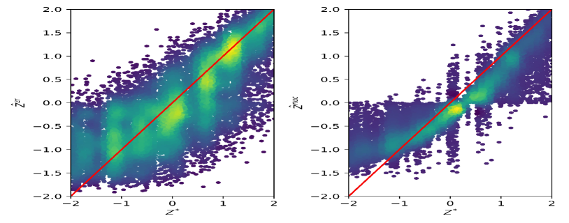
(a)

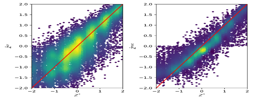
(b)

Figure 1: Scatter plots showing comparision of shrinkage of entries between $\hat{\mathbf{Z}}^{\rm zr}$ and $\hat{\mathbf{Z}}^{\rm nuc}$. Two settings are from the low-rank settings in Table 1, Table 2. Two figures in (1(a)) correspond to the setting with $\gamma=3$, $p=50$ and other two figures in (1(b)) correspond to the setting with $\gamma=5$, $p=50$.

5.2 Approximate low-rank simulation settings

For the approximation low-rank settings, we try to identify a data generating procedure different from the exact low-rank settings in section 5.1. As we explained in the beginning of section 5, it suffices to focus on generating procedure of clr matrices $\mathbf{Z}^{*}$. Different from Section section 5.1, we put $r=\min\{n,p\}$ but have $\mathbf{Z}^{*}=\tilde{\mathbf{U}}\mathbf{D}\tilde{\mathbf{V}}^{T}$ (instead of $\mathbf{Z}^{*}=\mathbf{U}\mathbf{V}^{T}$) where

1. $\tilde{\mathbf{U}}\in{\rm I\!R}^{n\times r}$, $\tilde{\mathbf{V}}\in{\rm I\!R}^{p\times r}$ are (column-wise $\ell_{2}$ normalized) right eigenvectors of $\mathbf{U}\in{\rm I\!R}^{n\times r}$, $\mathbf{V}\in{\rm I\!R}^{p\times\min\{n,p\}}$ to ensure diagonals of $\mathbf{D}$ can represent singular values of $\mathbf{Z}^{*}$.

2. $\mathbf{D}={\rm diag}\left\{i^{-2},i=1,2,\ldots,\min\{n,p\}\right\}$ satisfy approximate low-rank assumption (9) with $q=1$ (since $\displaystyle\sum_{i=1}^{\infty}i^{-2}=\frac{6}{\pi^{2}}<\infty$)

3. generate $\mathbf{U}\in{\rm I\!R}^{n\times r}$ and $\mathbf{V}=0,2\mathbf{V}^{(1)}+\mathbf{V}^{(2)}\in{\rm I\!R}^{p\times r}$ in the following way:

   $$\mathbf{V}^{(1)}_{ij}=\left\{\begin{array}[]{cc}1,&i=j;\\ v,&i\neq j\text{ with probability }q;\\ 1,&i\neq j\text{ with probability }1-q.\end{array}\right.,\mathbf{V}^{(2)}_{ij}\sim{\cal N}\left(0,5\cdot 10^{-2}\right),$$

   where the choice of $(v,q)$ is specified in Table 3 and this choice is the same for approximate low-rank settings in Table 1.

Further steps of generating count matrices ${\mathbf{W}}^{*}$ are specified in the beginning of section 5.

Table 3: Approximate low-rank simulation settings: comparison of estimation errors measured by $\sin\Theta$ distance for right singular subspaces for $\hat{\mathbf{Z}}^{\rm nuc}$, $\hat{\mathbf{Z}}^{zr}$ and $\hat{\mathbf{Z}}^{svt}$ in the low rank model over 50 replications (we run 50 replications since this is much slower than ”low-rank” settings). Data generating procedure follows section 5 with $(v,q)=(-1,0.5)$ in Section 5.2. This data generating procedure is the same as for approximate low-rank settings in Table 1.

	$p=50$			$p=100$			$p=150$
$\gamma$	$\widehat{\mathbf{V}}^{\rm nuc}$	$\widehat{\mathbf{V}}^{\rm zr}$	$\widehat{\mathbf{V}}^{\rm svt}$	$\widehat{\mathbf{V}}^{\rm nuc}$	$\widehat{\mathbf{V}}^{\rm zr}$	$\widehat{\mathbf{V}}^{\rm svt}$	$\widehat{\mathbf{V}}^{\rm nuc}$	$\widehat{\mathbf{V}}^{\rm zr}$	$\widehat{\mathbf{V}}^{\rm svt}$
$\left\|\sin\Theta\right\|_{F}^{2}$ $\left(\times 10^{-2}\right)$ $\widehat{\mathbf{V}}^{\rm nuc}$, $\widehat{\mathbf{V}}^{\rm zr}$, $\widehat{\mathbf{V}}^{\rm svt}\in{\rm I\!R}^{p\times 1}$
1	170.96	172.75	173.88	177.80	186.74	170.86	187.33	184.54	188.53
2	180.30	175.97	182.29	179.70	182.22	180.70	188.56	186.28	187.65
3	175.88	178.53	169.75	180.56	177.31	180.01	188.24	186.55	187.24
4	180.29	180.16	175.62	183.38	184.16	185.00	186.80	187.23	188.73
5	176.49	180.79	175.45	187.91	182.89	182.60	184.18	188.16	189.31
$\left\|\sin\Theta\right\|_{F}^{2}$ $\left(\times 10^{-2}\right)$ $\widehat{\mathbf{V}}^{\rm nuc}$, $\widehat{\mathbf{V}}^{\rm zr}$, $\widehat{\mathbf{V}}^{\rm svt}\in{\rm I\!R}^{p\times 2}$
1	333.34	331.12	339.27	351.64	347.54	345.49	361.45	362.41	358.81
2	329.49	333.59	337.45	350.35	352.69	352.94	363.64	359.81	360.31
3	338.77	343.03	333.04	353.88	349.34	350.01	364.20	357.38	365.85
4	343.73	343.84	334.12	353.46	356.75	355.17	363.32	367.29	365.61
5	331.76	334.34	342.92	357.04	353.80	357.61	358.72	361.38	368.84
$\left\|\sin\Theta\right\|_{F}^{2}$ $\left(\times 10^{-2}\right)$ $\widehat{\mathbf{V}}^{\rm nuc}$, $\widehat{\mathbf{V}}^{\rm zr}$, $\widehat{\mathbf{V}}^{\rm svt}\in{\rm I\!R}^{p\times 3}$
1	464.15	488.80	472.40	512.67	507.97	507.28	527.99	522.48	525.37
2	478.23	480.28	477.62	510.23	506.52	512.77	526.78	531.88	528.96
3	468.29	491.70	472.51	513.62	508.42	517.00	527.73	530.37	530.40
4	488.29	486.52	480.52	505.49	517.41	515.26	536.24	536.76	531.08
5	477.98	472.42	484.11	522.21	518.09	512.62	524.05	531.84	536.62
$\left\|\sin\Theta\right\|_{F}^{2}$ $\left(\times 10^{-1}\right)$ $\widehat{\mathbf{V}}^{\rm nuc}$, $\widehat{\mathbf{V}}^{\rm zr}$, $\widehat{\mathbf{V}}^{\rm svt}\in{\rm I\!R}^{p\times 20}$
1	174.99	175.57	175.69	243.59	243.28	244.26	276.34	276.72	275.47
2	176.66	176.13	178.83	246.08	246.03	244.15	274.31	273.95	275.32
3	179.43	176.85	176.68	246.70	244.33	244.78	275.04	275.88	274.45
4	176.39	176.49	177.03	247.01	247.38	247.75	275.19	276.05	275.95
5	177.19	173.74	175.30	244.59	247.42	245.51	274.97	275.03	275.58

We can see improvement in terms of estimation of $\hat{\mathbf{Z}}^{\rm nuc}$ in Table 1 but not much improvement $\hat{\mathbf{V}}^{\rm nuc}$ in Table 3. While in exact low-rank settings, we have already seen that estimation of singular spaces are more difficult than estimating clr matrix $\mathbf{Z}^{*}$, here such phenomena appear again in the approximate low-rank settings.

6 Analysis of Real Datasets

We apply our clr matrix estimation algorithm in section 3 to two real datasets, the gut microbiome data set in a cohort of 98 individuals [38] and the data set from the American Gut Project [29].

6.1 Gut Microbiome Dataset

The gut microbiome plays an important role in regulating metabolic functions and influences human health and disease [30, 39]. [38] reported a cohort gut microbiome data set that includes the counts of $87$ bacteria for $98$ healthy volunteers.

Fig. 2 shows the decay singular values $\hat{\mathbf{Z}}^{\rm zr}$ indicating an approximate low-rank clr matrix.

Fig. 3 shows boxplots for clr matrices $\hat{\mathbf{Z}}^{\rm zr}$, $\hat{\mathbf{Z}}^{\rm nuc}$. To compare the results, define

$$\Omega=\{(i,j):i=1,\ldots,n;j=1,\ldots,p|W_{ij}>0\}$$ (12)

and $\Omega^{c}$ as the support of the nonzero and zero entries in ${\mathbf{W}}$, respectively. Similar to [8], Fig. (3(b)) shows that the observed nonzero counts have an effect on estimating the clr matrix of the genera that were observed as zeros. The estimated centered-log-ratio $\hat{Z}_{ij}^{\rm nuc}$ in $\Omega^{c}$ tends to shrink towards those in $\Omega$. In contrast, the zero-replacement estimator $\hat{\mathbf{Z}}^{\rm zr}$ in Fig. (3(a)) provides almost the same estimates for all the samples/taxa in $\Omega^{c}$ and $\{W_{ij}\}_{(i,j)\in\Omega}$, i.e. the observed nonzero counts have little effect on $\left\{\hat{Z}_{ij}^{\rm zr}\right\}_{(i,j)\in\Omega^{c}}$.

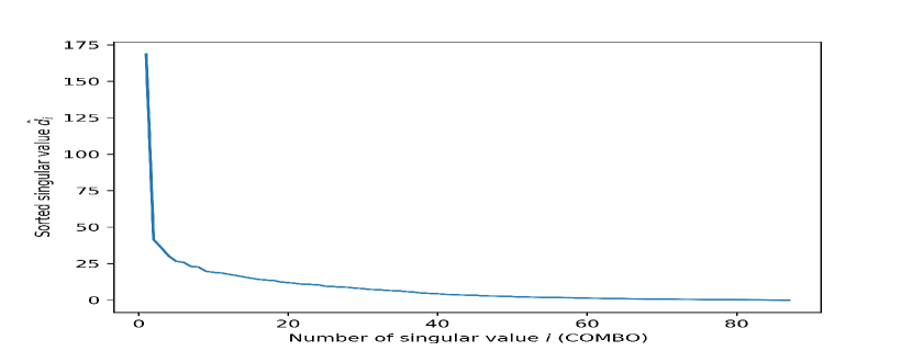
Figure 2: Analysis of Gut Microbime dataset. The plot shows the decay of singular values $\hat{d}_{i}$ (versus $i$) based on the singular value decomposition of $\hat{\mathbf{Z}}^{\rm nuc}=\hat{\mathbf{U}}^{\rm nuc}{\rm diag}\{\hat{d}_{1},\ldots,\hat{d}_{\min\{n,p\}}\}\left[\hat{\mathbf{V}}^{\rm nuc}\right]^{T}$ , indicating the low-rank structure of the compositional matrix.

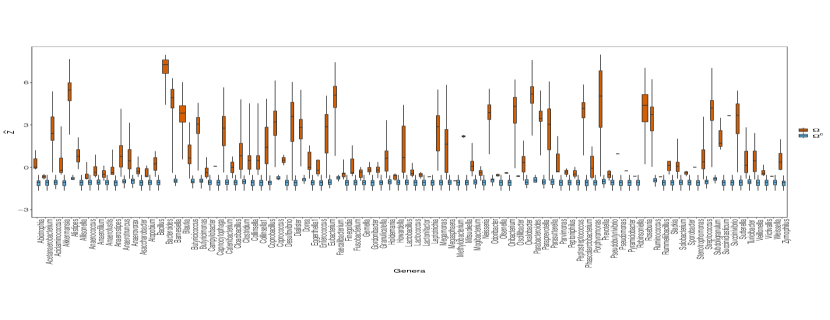
(a)

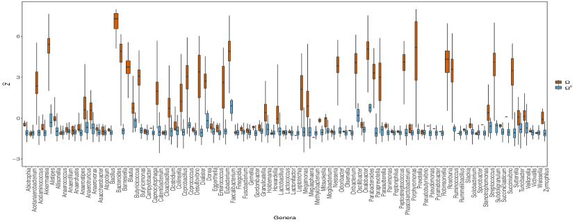
(b)

Figure 3: Analysis of the gut microbiome dataset of [38]. Boxplots of the estimated center log-ratio transformation for the genera corresponding to non-zero observations ($\Omega$) and zero observations ($\Omega^{c}$). Fig. 3(a): the zero replacement estimator $\widehat{\mathbf{Z}}^{\rm zr}$. Fig. 3(b): the proposed estimator $\widehat{\mathbf{Z}}^{\text{auto}}$ with tuning parameter set following section 3.3 where the tuning parameter is auto-tuned as $\lambda=2.15$.

6.2 American Gut Project

The microbiome data of the American Gut Project [29] includes the counts of $70$ bacteria for $3,566$ individuals collected through an open platform for citizen science. Fig. 4 shows the decay of singular values $\hat{\mathbf{Z}}^{\rm zr}$ indicating an approximate low-rank composition matrix.

Fig. 5 shows the boxplots of the estimated clr matrices $\hat{\mathbf{Z}}^{\rm zr}$, $\hat{\mathbf{Z}}^{\rm nuc}$ ordered by their columns. To compare the results, Fig. (5(b)) shows that the observed nonzero counts have much more effect on estimating the centered-log-ratio $Z_{ij}^{*}$ of the genera that were observed as zeros than $\hat{\mathbf{Z}}^{\rm zr}$ in Fig. (5(a)).

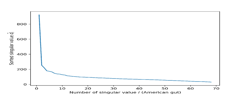
Figure 4: Analysis of the American Gut Project dataset: Fig. (4) shows decay of singular values $\hat{d}_{i}$ (versus $i$) based on the singular value decomposition of $\hat{\mathbf{Z}}^{\rm nuc}=\hat{\mathbf{U}}^{\rm nuc}{\rm diag}\{\hat{d}_{1},\ldots,\hat{d}_{\min\{n,p\}}\}\left[\hat{\mathbf{V}}^{\rm nuc)}\right]^{T}$ , indicating the low-rank structure of the compositional matrix.

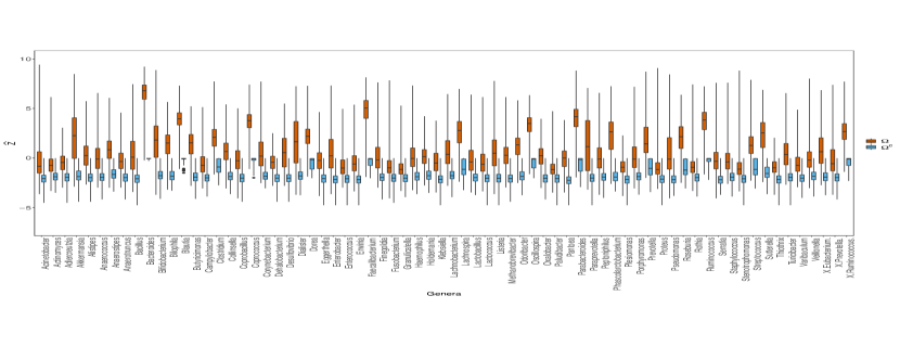
(a)

(b)

Figure 5: Analysis of the American Gut Project dataset, showing the boxplots of the estimated center log-ratio transformation of the compositions for the genera corresponding to non-zero observations ($\Omega$) and zero observations ($\Omega^{c})$ in combo data set. Top panel: the zero replacement estimator $\widehat{\mathbf{Z}}^{\rm zr}$. Bottom panel: the proposed estimator $\hat{\mathbf{Z}}^{\text{auto}}$ with the tuning parameter set following section 3.3, where the tuning parameter is auto-tuned as $\lambda=5.99$.

7 Discussion

Centroid-log-ratio transformation is one of the most commonly used tranformations in compositonal data analysis. Traditionally the centroid-log-ratios are estimated from the compositional vectors. However, in many studies such as microbiome studies that motivated our method in this paper, the raw data are counts instead of the compositions, let alone centroid-log-ratios. Treating the centroid-log-ratios as a parameter in Poisson-multinomial model for high dimensional count data, we have developed a nuclear-norm penalized maximum likelihood method for estimating the clr matrix of all the samples. The method effectively borrows information across the samples and taxa in order to achieve better estimation. We rarahave demonstrated this using simulations and analysis of the large real datasets of Gut Microbiome Dataset and the American Gut Project.The method can be efficiently implemented using the generalized accelerated proximal gradient method.

Supplementary Material

Supplementary material related to this article can be found online.

.1 Details of the algorithms

This section provides more details of the algorithms described in section 3.2 and section 3.3.

Algorithm 1 (denoted by ${NuclearCLR}\left({\mathbf{W}},\lambda\right)$ ) provides more details than those appeared in section 3.2, the generalized accelerated proximal gradient algorithm solving (2) with fixed tuning parameter $\lambda$.

0:  Count matrix ${\mathbf{W}}\in{\rm I\!N}^{n\times p}$, tuning parameter $\lambda$.

Auxiliary parameters: scaling parameter $\gamma_{L}=1.5$, initial step size $L_{0}$, friction rate $\rho=5$, zero-criterion parameter $\epsilon_{\{\mathcal{F}_{L}=0\}}=10^{-7}$; maximum number of iterations $K_{L,\max}=10^{4}$.

0:  Estimator of centroid log ratio matrix $\hat{\mathbf{Z}}^{(k)}\in{\rm I\!R}^{n\times p}$.

  Initialize $k=0$;

  (3): $\hat{Z}_{ij}^{(0)}=\hat{Y}_{ij}^{(0)}={\text{softmax}}\left(\frac{W_{ij}\wedge 0.5}{\sum_{j=1}^{p}\left(W_{ij}\wedge 0.5\right)}\right)+\epsilon$, where $\epsilon$ is the random perturbation with $\epsilon=\tilde{\epsilon}\cdot\left(\mathbf{I}_{p}-\frac{1}{p}{\bf 1}_{p}{\bf 1}_{p}\right)$ (and run $4,8,16,\ldots$ initializers due to this perturbation) ;

  while $k\leq K_{L,\max}$ do

     $k\leftarrow k+1$;

     Determine $\hat{\mathbf{Z}}^{(k)}$, $\hat{\mathbf{Y}}^{(k)}$ by (3.2), (4) in the following way:

     Set $L_{k}\leftarrow L_{0}$;

     while True  do

        (3.2) $\displaystyle\hat{\mathbf{Z}}^{(k)}\in\arg\min_{\mathbf{Z}\in{\rm I\!R}^{n\times p}}\frac{L_{k-1}}{2}\left\|\mathbf{Z}-\hat{\mathbf{Z}}^{(k-1)}+L_{k-1}^{-1}\nabla\mathcal{L}_{N}\left(\hat{\mathbf{Y}}^{(k-1)};{\mathbf{W}}\right)\right\|_{2}^{2}+\lambda\left\|\mathbf{Z}\right\|_{*}$ by SVD and singular value thresholding;

        (4) $\hat{\mathbf{Y}}^{(k)}\leftarrow\hat{\mathbf{Z}}^{(k)}+\frac{k-1}{k+\rho-1}\left(\hat{\mathbf{Z}}^{(k)}-\hat{\mathbf{Z}}^{(k-1)}\right)$;

        if $\mathcal{F}_{L_{k}}\left(\hat{\mathbf{Z}}^{(k)},\hat{\mathbf{Y}}^{(k)};{\mathbf{W}}\right)<0$ then

           break;

        end if

        $L_{k}\leftarrow\gamma_{L}L_{k}$.

     end while

     if $\left|\mathcal{F}_{L_{k}}\left(\hat{\mathbf{Z}}^{(k)},\hat{\mathbf{Y}}^{(k)};{\mathbf{W}}\right)\right|\leq\epsilon_{\{\mathcal{F}_{L}=0\}}$ then

        return $\hat{\mathbf{Z}}^{(k)}$; (exit)

     end if

  end while

  return $\hat{\mathbf{Z}}^{(k)}$; (exit)

Algorithm 1 ${NuclearCLR}\left({\mathbf{W}},\lambda\right)$, the algorithm described in Section 3.1 for (2).

Algorithm 2 provides more details than those appeared in Section 3.3 on how to process auto-tuning. The procedure is based on ${NuclearCLR}\left({\mathbf{W}},\lambda\right)$, that is, Algorithm 1.

0:  Count matrix ${\mathbf{W}}\in{\rm I\!N}^{n\times p}$.

Auxiliary parameters: maximum number of iterations $K_{\lambda,\max}=100$, stop criterion $\epsilon_{\lambda}=10^{-3}$, scaling parameter $\gamma_{\lambda}=1.2$.

0:  Estimator of centroid log ratio matrix $\hat{\mathbf{Z}}^{\text{auto}}\in{\rm I\!R}^{n\times p}$; selected tuning parameter $\lambda^{\text{auto}}$.

  Initialize $k=0$;

  (3): $\hat{Z}_{ij}^{(0)}=\hat{Y}_{ij}^{(0)}={\text{softmax}}\left(\frac{W_{ij}\wedge 0.5}{\sum_{j=1}^{p}\left(W_{ij}\wedge 0.5\right)}\right)$;

  $\lambda^{(1)}\leftarrow\mathcal{L}_{N}\left(\hat{\mathbf{Z}}^{(0)};{\mathbf{W}}\right)$;

  $\lambda^{\text{auto}}\leftarrow\lambda^{(1)}$;

  criterion $R\leftarrow\frac{\mathcal{L}_{N}\left(\hat{\mathbf{Z}}^{(0)};{\mathbf{W}}\right)}{\left\|\mathbf{Z}^{(0)}\right\|_{*}}+\frac{\left\|\hat{\mathbf{Z}}^{(0)}\right\|_{*}}{\mathcal{L}_{N}\left(\hat{\mathbf{Z}}^{(0)};{\mathbf{W}}\right)}$;

  while $k\leq K_{\lambda,\max}$ do

     $k\leftarrow k+1$;

     $\hat{\mathbf{Z}}^{(k)}\leftarrow\mathfrak{NuclearCLR}\left({\mathbf{W}},\lambda^{(k)}\right)$, that is, Algorithm 1;

     temporal $r\leftarrow\frac{\mathcal{L}_{N}\left(\hat{\mathbf{Z}}^{(k)};{\mathbf{W}}\right)}{\left\|\hat{\mathbf{Z}}^{(k)}\right\|_{*}}+\frac{\left\|\hat{\mathbf{Z}}^{(k)}\right\|_{*}}{\mathcal{L}_{N}\left(\hat{\mathbf{Z}}^{(k)};{\mathbf{W}}\right)}$;

     if $\frac{\left|R-r\right|}{R+r}\leq\epsilon_{\lambda}$ then

        $\lambda^{\text{auto}}\leftarrow\lambda^{(k)}$

        $\hat{\mathbf{Z}}^{\text{auto}}\leftarrow\mathfrak{NuclearCLR}\left({\mathbf{W}},\lambda^{\text{auto}}\right)$;

        return $\hat{\mathbf{Z}}^{\text{auto}}$, $\lambda^{\text{auto}}$; (exit)

     end if

     if $R>r$ then

        $R\leftarrow r$;

        $\lambda^{\text{auto}}\leftarrow\lambda^{(k)}$;

        $\lambda^{(k+1)}\leftarrow\lambda^{(k)}*\gamma$;

     else

        $\lambda^{(k+1)}\leftarrow\sqrt{\lambda^{(k)}\lambda^{\text{auto}}}$

     end if

  end while

  $\hat{\mathbf{Z}}^{\text{auto}}\leftarrow\mathfrak{NuclearCLR}\left({\mathbf{W}},\lambda^{\text{auto}}\right)$;

  return $\hat{\mathbf{Z}}^{\text{auto}}$, $\lambda^{\text{auto}}$; (exit)

Algorithm 2 Auto-tuning algorithm described in Section 3.3

.2 Proof of Theorems

For any integer $n>0$, we write $[n]=\{1,\ldots,n\}$ and denote ${\mathbf{e}}_{i}(n)$ as the canonical basis in ${\rm I\!R}^{n}$ with $i$th entry being one and others being zero.

Before our derivation, we present Lemma 5, which is a consequence of Davis-Kahan $\sin\Theta$ theorem. While some classical forms are in [33, 13], we present Davis-Kahan $\sin\Theta$ theorem in the context of our setting, which is analogous to [19]:

Lemma 5 (Davis-Kahan $\sin\Theta$).

Denote singular value decomposition of symmetric matrix $\hat{\mathbf{A}}_{m}\in{\rm I\!R}^{n\times n}$ as $\hat{\mathbf{A}}_{n}=\mathbf{V}_{\hat{\mathbf{A}}_{n}}{\Sigma}_{\hat{\mathbf{A}}_{n}}\mathbf{V}_{\hat{\mathbf{A}}_{n}}^{T}+\mathbf{V}_{\hat{\mathbf{A}}_{n}}^{\perp}{\Sigma}_{\hat{\mathbf{A}}_{n}}^{\perp}\left(\mathbf{V}_{\hat{\mathbf{A}}_{n}}^{\perp}\right)^{T}$, and similarly for $\mathbf{Z}_{n}$. Suppose $\left\|{\Sigma}_{\hat{\mathbf{A}}_{n}}^{\perp}\right\|_{2}<\left\|{\Sigma}_{\mathbf{A}_{n}}^{-1}\right\|_{2}^{-1}$, where $\left\|{\Sigma}_{\mathbf{A}_{n}}^{-1}\right\|_{2}^{-1}$ is the $r$th (absolutely) largest eigenvalue of $\mathbf{A}_{n}$, $\left\|{\Sigma}_{\hat{\mathbf{A}}_{n}}\right\|_{2}$ is the $(r+1)$th (absolutely) largest eigenvalue of $\hat{\mathbf{A}}_{n}$. Then for any unitarily-invariant norm $\|\cdot\|_{\mathcal{U}}$ (and we focus on $\|\cdot\|_{\mathcal{U}}=\|\cdot\|_{2},\|\cdot\|_{F}$),

$$\left\|\left(\mathbf{V}_{\hat{\mathbf{A}}_{n}}^{\perp}\right)^{T}\mathbf{V}_{\mathbf{A}_{n}}\right\|_{\mathcal{U}}\leq\frac{\left\|\left(\hat{\mathbf{A}}_{n}-\mathbf{A}_{n}\right)\mathbf{V}_{\mathbf{A}_{n}}\right\|_{\mathcal{U}}}{\left\|{\Sigma}_{\mathbf{A}_{n}}^{-1}\right\|_{2}^{-1}-\left\|{\Sigma}_{\hat{\mathbf{A}}_{n}}^{\perp}\right\|_{2}}=O_{P}\left(\frac{\left\|\hat{\mathbf{A}}_{n}-\mathbf{A}_{n}\right\|_{\mathcal{U}}}{\sigma_{r}\left(\mathbf{A}_{n}\right)}\right).$$

.2.1 Proof of Theorem 1 and Theorem 3

Theorem 1 and Theorem 3 can be considered as two special cases of following theorem:

Theorem 6 (Upper bounds).

With tuning parameter selected as (8)

$$\lambda=\delta\frac{\beta_{\mathbf{R}}\vee\left(p\max_{i,j}{\mathbf{X}}_{ij}^{*}\right)}{\left(p\min_{i,j}{\mathbf{X}}_{ij}^{*}\right)^{2}}\cdot\frac{\log(n+p)}{N},$$

$$\frac{1}{n}\left\|\mathbf{Z}^{*}-\hat{\mathbf{Z}}\right\|_{F}^{2}$$

$$\leq \frac{C}{\min_{i,j}{\text{softmax}}(\mathbf{Z}_{i}^{*})_{j}}$$

$$\cdot\left\{\left[\frac{\beta_{\mathbf{R}}\vee\left(\max_{i,j}{\text{softmax}}(\mathbf{Z}_{i}^{*})_{j}p\right)}{\left(\min_{i,j}{\text{softmax}}(\mathbf{Z}_{i}^{*})_{j}p\right)^{2}}\cdot\frac{\log(n+p)}{N}\right]^{\frac{1}{2}}\sum_{i=r+1}^{n\wedge p}\sigma_{i}\left(\mathbf{Z}^{*}\right)\right.$$

$$\left.+{\color[rgb]{0,0,0}\frac{\left[\max_{i,j}{\text{softmax}}(\mathbf{Z}^{*})\right]^{2}\cdot\left[\beta_{\mathbf{R}}\vee\left(\max_{i,j}{\text{softmax}}(\mathbf{Z}^{*})p\right)\right]}{\alpha_{\mathbf{R}}\left[\min_{i,j}{\text{softmax}}(\mathbf{Z}^{*})\right]^{3}}\cdot\frac{r(n+p)\log(n+p)}{pN}}\right\},$$

$$\frac{p}{n}\left\|{\text{softmax}}\left(\mathbf{Z}_{i}^{*}\right)-{\text{softmax}}\left(\hat{\mathbf{Z}}\right)\right\|_{F}^{2}$$

$$\leq C\left\{\left[\frac{\left[\max_{i,j}{\text{softmax}}(\mathbf{Z}^{*})\right]^{4}[\beta_{\mathbf{R}}\vee\left(\max_{i,j}{\text{softmax}}(\mathbf{Z}_{i}^{*})_{j}p\right)]}{\left(\min_{i,j}{\text{softmax}}(\mathbf{Z}_{i}^{*})_{j}p\right)^{4}}\cdot\frac{\log(n+p)}{N}\right]^{\frac{1}{2}}\sum_{i=r+1}^{n\wedge p}\sigma_{i}\left(\mathbf{Z}^{*}\right)\right.$$

$$\left.+{\color[rgb]{0,0,0}\frac{\left[\max_{i,j}{\text{softmax}}(\mathbf{Z}^{*})\right]^{4}\cdot\left[\beta_{\mathbf{R}}\vee\left(\max_{i,j}{\text{softmax}}(\mathbf{Z}^{*})p\right)\right]}{\alpha_{\mathbf{R}}\left[\min_{i,j}{\text{softmax}}(\mathbf{Z}^{*})\right]^{4}}\cdot\frac{r(n+p)\log(n+p)}{pN}}\right\},$$

In addition, given a fixed constant $C_{0}\geq\frac{6}{p\min_{i,j}{\text{softmax}}(\mathbf{Z}_{i}^{*})_{j}\alpha_{\mathbf{R}}}$, if $N<C_{0}(n+p)^{2}\log(n+p)$, we have

$$\frac{1}{n}\sum_{i=1}^{n}D_{KL}\left(\mathbf{Z}^{*},\hat{\mathbf{Z}}\right)$$

$$\leq C\left\{\left[\frac{\beta_{\mathbf{R}}\vee\left(\max_{i,j}{\text{softmax}}(\mathbf{Z}_{i}^{*})_{j}p\right)}{\left(\min_{i,j}{\text{softmax}}(\mathbf{Z}_{i}^{*})_{j}p\right)^{2}}\cdot\frac{\log(n+p)}{N}\right]^{\frac{1}{2}}\sum_{i=r+1}^{n\wedge p}\sigma_{i}\left(\mathbf{Z}^{*}\right)\right.$$

$$\left.+{\color[rgb]{0,0,0}\frac{\left[\max_{i,j}{\text{softmax}}(\mathbf{Z}^{*})\right]^{2}\cdot\left[\beta_{\mathbf{R}}\vee\left(\max_{i,j}{\text{softmax}}(\mathbf{Z}^{*})p\right)\right]}{\alpha_{\mathbf{R}}\left[\min_{i,j}{\text{softmax}}(\mathbf{Z}^{*})\right]^{3}}\cdot\frac{r(n+p)\log(n+p)}{pN}}\right\}.$$

with probability at least $1-\frac{3}{n+p}$.

Proof.

Similar to [8], the count matrix ${\mathbf{W}}$ follows a multinomial distribution: ${\mathbf{W}}=\sum_{k=1}^{N}\mathbf{E}_{k}$ where $\mathbf{E}_{k}$ are independent and identically distributed copies of a Bernoulli random matrix $\mathbf{E}$ that satisfies

$${\mathbf{P}}\left(\mathbf{E}={\mathbf{e}}_{i}(n){\mathbf{e}}_{j}(p)^{T}=\left[\mathbf{R}\cdot{\bf 1}_{p}^{T}\cdot{\text{softmax}}\left(\mathbf{Z}^{*}\right)\right]_{ij}\right),$$

where $\mathbf{R}$ is specified in section 4.

Consequentially,

$$\mathcal{L}_{N}(\mathbf{Z}) = -\frac{1}{N}\sum_{k=1}^{N}\log\langle{\text{softmax}}(\mathbf{Z}),\mathbf{E}_{k}\rangle=-\frac{1}{N}\sum_{k=1}^{N}\log\langle{\text{softmax}}(\mathbf{Z}),\mathbf{E}_{k}\rangle$$ (13)

$$= -\frac{1}{N}\sum_{k=1}^{N}\sum_{i=1}^{n}\log\langle{\mathbf{e}}_{i}(n){\mathbf{e}}_{i}(n)^{T}{\text{softmax}}(\mathbf{Z}),\mathbf{E}_{k}\rangle$$

$$= -\frac{1}{N}\sum_{i=1}^{n}\sum_{k=1}^{N}\log\langle{\text{softmax}}(\mathbf{Z}_{i})^{T},\ \mathbf{E}_{k}^{T}e_{i}(n)\rangle.$$

Any solution $\hat{\mathbf{Z}}$ to (2) satisfies

$$\mathcal{L}_{N}\left(\hat{\mathbf{Z}}\right)-\mathcal{L}_{N}\left(\mathbf{Z}^{*}\right)$$ (14)

$$= \frac{1}{N}\sum_{i=1}^{n}\sum_{j=1}^{p}\left[W_{ij}\log\left({\text{softmax}}\left(\mathbf{Z}_{i}^{*}\right)_{j}\right)-W_{ij}\log\left({\text{softmax}}\left(\hat{\mathbf{Z}}_{i}\right)_{j}\right)\right]$$

$$\leq \lambda\left(\left\|\mathbf{Z}^{*}\right\|_{*}-\left\|\hat{\mathbf{Z}}\right\|_{*}\right).$$

Next we present following Lemmas to derive a lower bound for (13):

Lemma 7.

Given the selected tuning parameter from Theorem 6, with probability at least $1-\frac{1}{n+p}$, we have the following upper bound for $\left\|\mathbf{Z}^{*}-\hat{\mathbf{Z}}\right\|_{*}$:

$$\left\|\mathbf{Z}^{*}-\hat{\mathbf{Z}}\right\|_{*}\leq 4\sqrt{2r}\left\|\mathbf{Z}^{*}-\hat{\mathbf{Z}}\right\|_{F}+4\sum_{i=r+1}^{n\wedge p}\sigma_{i}\left(\mathbf{Z}^{*}\right).$$ (15)

Lemma 8.

If $\mathbf{Z}^{*}$ satisfies (15) as well as $\mathbf{Z}{\bf 1}_{p}={\vec{\mathbf{0}}}_{n}$, we have

$$\frac{1}{N}\sum_{i=1}^{n}R_{i}D_{KL}\left({\text{softmax}}\left(\mathbf{Z}_{i}^{*}\right),{\text{softmax}}\left(\hat{\mathbf{Z}}_{i}\right)\right)$$

$$\leq \mathcal{L}_{N}\left(\hat{\mathbf{Z}}\right)-\mathcal{L}_{N}\left(\mathbf{Z}^{*}\right)+C_{2}\frac{\beta_{\mathbf{R}}\vee\left(\max_{i,j}{\text{softmax}}(\mathbf{Z}_{i}^{*})_{j}p\right)}{\left(\min_{i,j}{\text{softmax}}(\mathbf{Z}_{i}^{*})_{j}p\right)^{2}}\cdot\frac{\log(n+p)}{N}\sum_{i=r+1}^{n\wedge p}\sigma_{i}\left(\mathbf{Z}^{*}\right)$$

$$+{\color[rgb]{0,0,0}C_{2}\frac{\left(\max_{i,j}{\text{softmax}}(\mathbf{Z}_{i}^{*})_{j}p\right)^{2}\cdot\left[\beta_{\mathbf{R}}\vee\left(\max_{i,j}{\text{softmax}}(\mathbf{Z}_{i}^{*})_{j}p\right)\right]}{\alpha_{\mathbf{R}}\left(\min_{i,j}{\text{softmax}}(\mathbf{Z}_{i}^{*})_{j}p\right)^{3}}\cdot\frac{r(n+p)\log(n+p)}{N}},$$

with probability proceeding $1-\frac{2}{n+p}$.

Lemma 9.

For any $\mathbf{Z},\hat{\mathbf{Z}}\in{\rm I\!R}^{n\times p}$ such that $\mathbf{Z}{\bf 1}_{p}=\hat{\mathbf{Z}}{\bf 1}_{p}={\vec{\mathbf{0}}}_{n}$, we have

$$\min_{i,j}X_{ij}^{*}\leq\frac{\sum_{i=1}^{n}D_{KL}\left({\text{softmax}}\left(\mathbf{Z}_{i}^{*}\right),{\text{softmax}}\left(\hat{\mathbf{Z}}_{i}\right)\right)}{\left\|\mathbf{Z}^{*}-\hat{\mathbf{Z}}\right\|_{F}^{2}}\leq\max_{i,j}X_{ij}^{*}.$$

1. First regime: $N<(n+p)\log(n+p)$, By applying Lemma 7, 9, we obtain the upper bound of $\|\mathbf{Z}^{*}\|_{*}-\|\hat{\mathbf{Z}}\|_{*}$ as

   $$\|\mathbf{Z}^{*}\|_{*}-\|\hat{\mathbf{Z}}\|_{*} \leq \|\mathbf{Z}^{*}-\hat{\mathbf{Z}}\|_{*}\leq 4\sqrt{2r}\|\hat{\mathbf{Z}}^{*}-\hat{\mathbf{Z}}\|_{F}+4\sum_{i=r+1}^{n\wedge p}\sigma_{i}\left(\mathbf{Z}^{*}\right)$$

   $$\leq \sqrt{\frac{\sum_{i=1}^{n}D_{KL}\left({\text{softmax}}\left(\mathbf{Z}_{i}^{*}\right),{\text{softmax}}\left(\mathbf{Z}_{i}^{*}\right)\right)}{n\min_{i,j}{\text{softmax}}(\mathbf{Z}_{i}^{*})_{j}}}+4\sum_{i=r+1}^{n\wedge p}\sigma_{i}\left(\mathbf{Z}^{*}\right).$$

   Therefore, combining (14), Lemma 7 and Lemma 8 imply

   $$\frac{\alpha_{\mathbf{R}}}{n}\sum_{i=1}^{n}D_{KL}\left({\text{softmax}}\left(\mathbf{Z}_{i}^{*}\right),{\text{softmax}}\left(\hat{\mathbf{Z}}_{i}\right)\right)$$

   $$\leq \frac{1}{N}\sum_{i=1}^{n}R_{i}D_{KL}\left({\text{softmax}}\left(\mathbf{Z}_{i}^{*}\right),{\text{softmax}}\left(\hat{\mathbf{Z}}_{i}\right)\right)$$

   $$\leq \lambda\left[\sqrt{\frac{\displaystyle\sum_{i=1}^{n}D_{KL}\left({\text{softmax}}\left(\mathbf{Z}_{i}^{*}\right),{\text{softmax}}\left(\hat{\mathbf{Z}}_{i}\right)\right)}{n\min_{i,j}{\text{softmax}}(\mathbf{Z}_{i}^{*})_{j}}}+4\sum_{i=r+1}^{n\wedge p}\sigma_{i}\left(\mathbf{Z}^{*}\right)\right]$$

   $$+\frac{\beta_{\mathbf{R}}\vee\left(\max_{i,j}{\text{softmax}}(\mathbf{Z}_{i}^{*})_{j}p\right)}{\left(\min_{i,j}{\text{softmax}}(\mathbf{Z}_{i}^{*})_{j}p\right)^{2}}\cdot\frac{\log(n+p)}{N}\sum_{i=r+1}^{n\wedge p}\sigma_{i}\left(\mathbf{Z}^{*}\right)$$

   $$+{\color[rgb]{0,0,0}C_{2}\frac{\left({\text{softmax}}(\mathbf{Z}^{*})p\right)^{2}\cdot\left[\beta_{\mathbf{R}}\vee\left({\text{softmax}}(\mathbf{Z}^{*})p\right)\right]}{\alpha_{\mathbf{R}}\left({\text{softmax}}(\mathbf{Z}^{*})p\right)^{3}}\cdot\frac{r(n+p)\log(n+p)}{N}},$$

   with probability at least $1-\frac{3}{n+p}$. The above formula can be treated as a quadratic inequality for $\displaystyle\sum_{i=1}^{n}D_{KL}\left({\text{softmax}}\left(\mathbf{Z}_{i}^{*}\right),{\text{softmax}}\left(\hat{\mathbf{Z}}_{i}\right)\right)$. We plug in $\lambda$ in Theorem 6, and obtain

   $$\frac{1}{n}\sum_{i=1}^{n}D_{KL}\left({\text{softmax}}\left(\mathbf{Z}_{i}^{*}\right),{\text{softmax}}\left(\hat{\mathbf{Z}}_{i}\right)\right)$$

   $$\leq C_{3}\left\{\frac{\beta_{\mathbf{R}}\vee\left(\max_{i,j}{\text{softmax}}(\mathbf{Z}_{i}^{*})_{j}p\right)}{\left(\min_{i,j}{\text{softmax}}(\mathbf{Z}_{i}^{*})_{j}p\right)^{2}}\cdot\frac{\log(n+p)}{N}\sum_{i=r+1}^{n\wedge p}\sigma_{i}\left(\mathbf{Z}^{*}\right)\right.$$

   $$\left.+{\color[rgb]{0,0,0}\frac{\left({\text{softmax}}(\mathbf{Z}^{*})p\right)^{2}\cdot\left[\beta_{\mathbf{R}}\vee\left({\text{softmax}}(\mathbf{Z}^{*})p\right)\right]}{\alpha_{\mathbf{R}}\left({\text{softmax}}(\mathbf{Z}^{*})p\right)^{3}}\cdot\frac{r(n+p)\log(n+p)}{N}}\right\}$$

2. Second regime: $N>C_{0}(n+p)\log(n+p)$. We denote $\triangle\doteq\hat{\mathbf{Z}}-\mathbf{Z}^{*}$. According to (13) and Taylor expansion, that is, there exists $t\in(0,1)$ such that

   $$\mathcal{L}_{N}\left(\hat{\mathbf{Z}}\right)-\mathcal{L}_{N}\left(\mathbf{Z}^{*}\right)-\left\langle\nabla\mathcal{L}_{N}\left(\hat{\mathbf{Z}}\right),\Delta\right\rangle$$

   $$= \frac{1}{N}vec(\Delta)^{T}vec\left(\nabla vec\left(\nabla\mathcal{L}_{N}\left(\hat{\mathbf{Z}}+t\mathbf{Z}^{*}\right)\right)\right)vec(\Delta)$$

   $$= \frac{1}{N}vec(\Delta)^{T}\sum_{i=1}^{n}vec\left(\nabla vec\left(\nabla\mathcal{L}_{N_{i}}\left(t\hat{\mathbf{Z}}+(1-t)\mathbf{Z}^{*}\right)\right)\right)vec(\Delta),$$

∎

.3 Proof of Lemmas

.3.1 Proof of Lemma 7

For notational simplicity, we denote $\Delta\triangleq\hat{\mathbf{Z}}-\mathbf{Z}^{*}\in{\rm I\!R}^{n\times p}$, and

$$\nabla\mathcal{L}_{N}(\mathbf{Z}) \triangleq \left(\frac{\partial\mathcal{L}_{N}}{\partial z_{ij}}\right)_{n\times p}=\left(\frac{N_{i}}{N}\cdot\frac{e^{z_{ij}}}{\displaystyle\sum_{k=1}^{p}e^{z_{ik}}}-\frac{W_{ij}}{N}\right)_{n\times p}\in{\rm I\!R}^{n\times p}$$ (16)

$$= \begin{bmatrix}\frac{N_{1}}{N}\nabla\mathcal{L}_{N_{1}}(\mathbf{Z}_{1})\\ \vdots\\ \frac{N_{n}}{N}\nabla\mathcal{L}_{N_{n}}(\mathbf{Z}_{n})\end{bmatrix}$$

$$\xlongequal{\text{\eqref{eq:MLE rewrite}}} -\frac{1}{N}\sum_{k=1}^{N}\begin{bmatrix}\frac{{\mathbf{e}}_{1}(n)^{T}\mathbf{E}_{k}\cdot\nabla{clr}^{-1}(\mathbf{Z}_{1})}{\langle{\text{softmax}}(\mathbf{Z}_{1})^{T},\mathbf{E}_{k}^{T}{\mathbf{e}}_{1}(n)\rangle}\\ \vdots\\ \frac{{\mathbf{e}}_{n}(n)^{T}\mathbf{E}_{k}\cdot\nabla{clr}^{-1}(\mathbf{Z}_{n})}{\langle{\text{softmax}}(\mathbf{Z}_{n})^{T},\mathbf{E}_{k}^{T}{\mathbf{e}}_{n}(n)\rangle}\end{bmatrix}=\begin{bmatrix}\frac{{\mathbf{e}}_{i}(n)^{T}\mathbf{E}_{k}\cdot\nabla{clr}^{-1}(\mathbf{Z}_{i})}{\langle{\text{softmax}}(\mathbf{Z}_{i})^{T},\mathbf{E}_{k}^{T}{\mathbf{e}}_{i}(n)\rangle}\end{bmatrix}_{i\in[n]},$$

Denote $vec(\Delta),vec(\nabla\mathcal{L}_{N})\in{\rm I\!R}^{np}$ vectorized forms of corresponding matrices. According to Taylor expansion,

$$\mathcal{L}_{N}\left(\hat{\mathbf{Z}}\right)-\mathcal{L}_{N}\left(\mathbf{Z}^{*}\right)-\left\langle\nabla\mathcal{L}_{N}\left(\hat{\mathbf{Z}}\right),\Delta\right\rangle$$ (17)

$$= \frac{1}{N}vec(\Delta)^{T}vec\left(\nabla vec\left(\nabla\mathcal{L}_{N}\left(\hat{\mathbf{Z}}+t\mathbf{Z}^{*}\right)\right)\right)vec(\Delta)$$

$$= \frac{1}{N}vec(\Delta)^{T}\sum_{i=1}^{n}vec\left(\nabla vec\left(\nabla\mathcal{L}_{N_{i}}\left(\hat{\mathbf{Z}}+t\mathbf{Z}^{*}\right)\right)\right)vec(\Delta),$$

and furtherly we obtain

$$0 \leq \frac{1}{N}vec(\Delta)^{T}\sum_{i=1}^{n}vec\left(\nabla vec\left(\nabla\mathcal{L}_{N_{i}}\left(\hat{\mathbf{Z}}+t\mathbf{Z}^{*}\right)\right)\right)vec(\Delta)$$

$$= \mathcal{L}_{N}\left(\hat{\mathbf{Z}}\right)-\mathcal{L}_{N}\left(\mathbf{Z}^{*}\right)-\left\langle\nabla\mathcal{L}_{N}\left(\hat{\mathbf{Z}}\right),\Delta\right\rangle$$

$$\leq -\left\langle\nabla\mathcal{L}_{N}\left(\hat{\mathbf{Z}}\right),\Delta\right\rangle+\lambda\left(\left\|\mathbf{Z}^{*}\right\|_{*}-\left\|\hat{\mathbf{Z}}\right\|_{*}\right)$$

$$\leq \left\|\nabla\mathcal{L}_{N}\left(\hat{\mathbf{Z}}\right)\right\|_{2}\cdot\left\|\Delta\right\|_{*}+\lambda\left(\left\|\mathbf{Z}^{*}\right\|_{*}-\left\|\hat{\mathbf{Z}}\right\|_{*}\right)$$

To further upper bound the nuclear norm $\|\hat{\mathbf{Z}}-\mathbf{Z}^{*}\|_{*}$, we state two technical results:

Lemma 10.

With probability at least $1-\frac{1}{n+p}$, we have

$$\left\|\nabla\mathcal{L}_{N}(\mathbf{Z}^{*})\right\|_{2}\leq\left[\frac{M}{3}+\sqrt{\frac{M^{2}}{9}+\frac{\sigma^{2}}{\log(n+p)}}\right]\frac{2\log(n+p)}{N}\leq c\frac{\log(n+p)}{N},$$

$\displaystyle\sigma^{2}=1-\sum_{i=1}^{n}\nu_{i}\left\|{\text{softmax}}\left(\mathbf{Z}_{i}^{*}\right)\right\|_{2}^{2}$,

$$M=\sqrt{1+\max_{i\in[n]}\left[\left\|{clr}^{-1}(\mathbf{Z}_{i}^{*})\right\|_{2}^{2}-2\min_{j\in[p]}{clr}^{-1}(\mathbf{Z}_{i}^{*})_{j}\right]}.$$

Based on Lemma 10, with probability proceeding $1-\frac{1}{n+p}$, the selected tuning parameter $\lambda\geq 2\left\|\nabla\mathcal{L}_{N}(\mathbf{Z}^{*})\right\|_{2}$.

According to Lemma 1 (B.2) in [31] as well as Lemma 5 in [8], we obtain Lemma 7.

Proof of Lemma 8

For notational simplicity, we denote

$$\eta \triangleq n\log\frac{\max_{i,j}X_{ij}^{*}}{\min_{i,j}X_{ij}^{*}}\left[\frac{512\log(n+p)}{\log 4\alpha_{\mathbf{R}}^{2}N}\right]^{\frac{1}{2}},$$

$$D_{\mathbf{R}}\left({\text{softmax}}\left(\mathbf{Z}^{*}\right),{\text{softmax}}(\mathbf{Z})\right) \triangleq \sum_{i=1}^{n}R_{i}D_{KL}\left({\text{softmax}}\left(\mathbf{Z}_{i}^{*}\right),{\text{softmax}}(\mathbf{Z}_{i})\right).$$

The main lines of this proof are in the same spirit as Lemma 2 in [8] as well as Lemma 3 in [31]. We use a peeling argument to prove the probability of the following ”bad” event is small:

$$\mathcal{B}\triangleq$$

$$\left\{\mathbf{Z}\in{\rm I\!R}^{n\times p}:\left|{\tiny\frac{1}{N}\sum_{k=1}^{N}\log\langle{\text{softmax}}(\mathbf{Z})-{\text{softmax}}\left(\mathbf{Z}^{*}\right),\mathbf{E}_{k}\rangle-D_{\mathbf{R}}\left({\text{softmax}}\left(\mathbf{Z}_{i}^{*}\right),{\text{softmax}}(\mathbf{Z}_{i})\right)}\right|\right.$$

$$\left.\geq D_{\mathbf{R}}\left({\text{softmax}}\left(\mathbf{Z}_{i}^{*}\right),{\text{softmax}}(\mathbf{Z}_{i})\right)+E(n,p,r)\right\},$$

where $E(n,p,r)$ is defined by

$$E(n,p,r)\triangleq$$ (18)

$$\left[\frac{\left[(\beta_{\mathbf{R}}/n)\vee\max_{i,j}X_{ij}^{*}\right]\log(n+p)}{N}+\frac{\log(n+p)}{N}\right]$$

$$\cdot\left\{\frac{2048\left[\max_{i,j}{\text{softmax}}(\mathbf{Z}_{i}^{*})_{j}\right]^{2}nr}{\left[\min_{i,j}{\text{softmax}}(\mathbf{Z}_{i}^{*})_{j}\right]^{3}\alpha_{\mathbf{R}}}\left(\frac{\max_{i,j}X_{ij}^{*}}{\min_{i,j}X_{ij}^{*}}\right)^{2}\right.$$

$$\cdot\left[\frac{\left[(\beta_{\mathbf{R}}/n)\vee\max_{i,j}X_{ij}^{*}\right]\log(n+p)}{N}\frac{\log(n+p)}{N}\right]$$ (19)

$$+\left.\frac{16}{\min_{i,j}{\text{softmax}}(\mathbf{Z}_{i}^{*})_{j}}\sum_{i=r+1}^{n\wedge p}\sigma_{i}\left(\mathbf{Z}^{*}\right)\right\},$$

We separate the constraint set $\{\mathbf{Z}:\mathbf{Z}{\bf 1}_{p}={\vec{\mathbf{0}}}_{n}\}$ into pieces and focus on a sequence of small sets:

$$\mathcal{C}_{l}\triangleq\left\{\mathbf{Z}:\mathbf{Z}{\bf 1}_{p}={\vec{\mathbf{0}}}_{n},2^{l-1}\eta\leq\sum_{i=1}^{n}D_{KL}\left({\text{softmax}}\left(\mathbf{Z}_{i}^{*}\right),{\text{softmax}}(\mathbf{Z}_{i})\right)\leq 2^{l}\eta\right\},l=1,2,3,\ldots$$

Notice

$$D_{\mathbf{R}}\left({\text{softmax}}\left(\mathbf{Z}^{*}\right),{\text{softmax}}(\mathbf{Z})\right)\geq\frac{\alpha_{\mathbf{R}}}{n}\sum_{i=1}^{n}D_{KL}\left({\text{softmax}}\left(\mathbf{Z}_{i}^{*}\right),{\text{softmax}}(\mathbf{Z}_{i})\right),$$

it suffices to estimate the probability of the following events and then apply the union bound,

$$\mathcal{B}_{l}\triangleq$$

$$\left\{\exists\mathbf{Z}:\left|\frac{1}{N}\sum_{k=1}^{N}\log\langle{\text{softmax}}(\mathbf{Z})-{\text{softmax}}\left(\mathbf{Z}^{*}\right),\mathbf{E}_{k}\rangle-D_{\mathbf{R}}\left({\text{softmax}}\left(\mathbf{Z}_{i}^{*}\right),{\text{softmax}}(\mathbf{Z}_{i})\right)\right|\right.$$

$$\left.\geq\frac{2^{l}\eta\alpha_{\mathbf{R}}}{4n}+E(n,p,r),\mathbf{Z}{\bf 1}_{p}={\vec{\mathbf{0}}}_{n}\right\},$$

Since $\mathcal{C}_{l}\subset\mathcal{D}(2^{l}\eta)\triangleq\left\{\mathbf{Z}:\mathbf{Z}{\bf 1}_{p}={\vec{\mathbf{0}}}_{n},D_{\mathbf{R}}\left({\text{softmax}}\left(\mathbf{Z}_{i}^{*}\right),{\text{softmax}}(\mathbf{Z}_{i})\right)\leq 2^{l}\eta\right\}$ we can establish the upper bound of the probability of event $\mathcal{B}$ by using the union bound, the fact that $x\geq\log x$ and Lemma 13:

$${\mathbf{P}}\left(\mathcal{B}\right) \leq \sum_{l=1}^{\infty}{\mathbf{P}}\left(\mathcal{D}(2^{l}\eta)\cap\mathcal{B}_{l}\right)$$

$$\leq \sum_{l=1}^{\infty}\exp\left[-\frac{\alpha_{\mathbf{R}}^{2}N\eta^{2}4^{l}}{512\left(n\log\frac{\max_{i,j}{\text{softmax}}\left(\mathbf{Z}_{i}^{*}\right)_{j}}{\min_{i,j}{\text{softmax}}\left(\mathbf{Z}_{i}^{*}\right)_{j}}\right)^{2}}\right]$$

$$\leq \sum_{l=1}^{\infty}\exp\left[-\frac{\alpha_{\mathbf{R}}^{2}N\eta^{2}l\log 4}{512\left(n\log\frac{\max_{i,j}{\text{softmax}}\left(\mathbf{Z}_{i}^{*}\right)_{j}}{\min_{i,j}{\text{softmax}}\left(\mathbf{Z}_{i}^{*}\right)_{j}}\right)^{2}}\right]$$

$$\leq \sum_{l=1}^{\infty}(n+p)^{-l}\leq\frac{2}{n+p}.$$

Note that by the conditions that $N>(n+p)\log(n+p)$, these exists some constant $C_{2}>0$ such that

$$E(n,p,r)$$

$$\leq C_{2}\frac{\beta_{\mathbf{R}}\vee\left(\max_{i,j}{\text{softmax}}(\mathbf{Z}_{i}^{*})_{j}p\right)}{\left(\min_{i,j}{\text{softmax}}(\mathbf{Z}_{i}^{*})_{j}p\right)^{2}}\cdot\frac{\log(n+p)}{N}\sum_{i=r+1}^{n\wedge p}\sigma_{i}\left(\mathbf{Z}^{*}\right)$$

$$+{\color[rgb]{0,0,0}C_{2}\frac{\left(\max_{i,j}{\text{softmax}}(\mathbf{Z}_{i}^{*})_{j}p\right)^{2}\cdot\left[\beta_{\mathbf{R}}\vee\left(\max_{i,j}{\text{softmax}}(\mathbf{Z}_{i}^{*})_{j}p\right)\right]}{\alpha_{\mathbf{R}}\left(\min_{i,j}{\text{softmax}}(\mathbf{Z}_{i}^{*})_{j}p\right)^{3}}\cdot\frac{r(n+p)\log(n+p)}{N}},$$

which completes the proof.

Proof of Lemma 9 By using Taylor expansion, we can rewrite KL divergence as

$$\sum_{i=1}^{n}D_{KL}\left({\text{softmax}}\left(\mathbf{Z}_{i}^{*}\right),{\text{softmax}}\left(\hat{\mathbf{Z}}_{i}\right)\right)$$

$$= \sum_{i=1}^{n}\left[\log\sum_{k=1}^{p}e^{\hat{z}_{ik}}-\log\sum_{k=1}^{p}e^{z_{ik}^{*}}-\sum_{j=1}^{p}{\text{softmax}}\left(\mathbf{Z}_{i}^{*}\right)_{j}\left(\hat{z}_{ij}-z_{ij}^{*}\right)\right]$$

$$= -\sum_{i=1}^{n}\left(\hat{\mathbf{Z}}_{i}-\mathbf{Z}_{i}^{*}\right)^{T}\nabla^{2}{\text{softmax}}\left((1-t)\mathbf{Z}_{i}^{*}+t\hat{\mathbf{Z}}_{i}\right)\left(\hat{\mathbf{Z}}_{i}-\mathbf{Z}_{i}^{*}\right),$$

where $\nabla^{2}{\text{softmax}}\left(\xi\right)=-{\rm diag}\left\{{\text{softmax}}(\xi)\right\}+{\text{softmax}}(\xi)^{T}{\text{softmax}}(\xi)$. Let us denote ${\mathbf{u}}\triangleq{\text{softmax}}\left(\xi\right)$ and then for any ${\mathbf{x}}\in{\rm I\!R}^{p}\setminus\{{\vec{\mathbf{0}}}_{p}\}$ such that ${\mathbf{x}}^{T}{\bf 1}_{p}=0$,

$$\frac{-{\mathbf{x}}^{T}\nabla^{2}{\text{softmax}}\left(\xi\right){\mathbf{x}}}{{\mathbf{x}}^{T}{\mathbf{x}}}=\frac{{\mathbf{x}}^{T}\left({\rm diag}({\mathbf{u}})-{\mathbf{u}}{\mathbf{u}}^{T}\right){\mathbf{x}}}{{\mathbf{x}}^{T}{\mathbf{x}}}$$

$$= \frac{\left({\rm diag}({\mathbf{u}})^{\frac{1}{2}}{\mathbf{x}}\right)^{T}\left(\mathbf{I}_{p}-{\rm diag}({\mathbf{u}})^{-\frac{1}{2}}{\mathbf{u}}\left[{\rm diag}({\mathbf{u}})^{-\frac{1}{2}}{\mathbf{u}}\right]^{T}\right){\rm diag}({\mathbf{u}})^{\frac{1}{2}}{\mathbf{x}}}{{\mathbf{x}}^{T}{\mathbf{x}}}$$

$$= \frac{\left({\rm diag}({\mathbf{u}})^{\frac{1}{2}}{\mathbf{x}}\right)^{T}\left(\mathbf{I}_{p}-{\rm diag}({\mathbf{u}})^{-\frac{1}{2}}{\mathbf{u}}\left[{\rm diag}({\mathbf{u}})^{-\frac{1}{2}}{\mathbf{u}}\right]^{T}\right){\rm diag}({\mathbf{u}})^{\frac{1}{2}}{\mathbf{x}}}{\left({\rm diag}({\mathbf{u}})^{\frac{1}{2}}{\mathbf{x}}\right)^{T}{\rm diag}({\mathbf{u}})^{\frac{1}{2}}{\mathbf{x}}}\cdot$$

$$\frac{\left({\rm diag}({\mathbf{u}})^{\frac{1}{2}}{\mathbf{x}}\right)^{T}{\rm diag}({\mathbf{u}})^{\frac{1}{2}}{\mathbf{x}}}{{\mathbf{x}}^{T}{\mathbf{x}}}$$

and thus

$$\min_{j}U_{J}\left(\xi\right)_{j}$$

$$= \min_{j}u_{j}\cdot\inf_{{\mathbf{y}}^{T}{\bf 1}_{p}=0}\frac{{\mathbf{y}}^{T}\left(\mathbf{I}_{p}-{\rm diag}({\mathbf{u}})^{-\frac{1}{2}}{\mathbf{u}}\left[{\rm diag}({\mathbf{u}})^{-\frac{1}{2}}{\mathbf{u}}\right]^{T}\right){\mathbf{y}}}{{\mathbf{y}}^{T}{\mathbf{y}}}$$

$$\leq \frac{-{\mathbf{x}}^{T}\nabla^{2}{\text{softmax}}\left(\xi\right){\mathbf{x}}}{{\mathbf{x}}^{T}{\mathbf{x}}}$$

$$\leq \max_{j}u_{j}\cdot\sup_{{\mathbf{y}}^{T}{\bf 1}_{p}=0}\frac{{\mathbf{y}}^{T}\left(\mathbf{I}_{p}-{\rm diag}({\mathbf{u}})^{-\frac{1}{2}}{\mathbf{u}}\left[{\rm diag}({\mathbf{u}})^{-\frac{1}{2}}{\mathbf{u}}\right]^{T}\right){\mathbf{y}}}{{\mathbf{y}}^{T}{\mathbf{y}}}$$

$$= \max_{j}{\text{softmax}}\left(\xi\right)_{j}.$$

As a result, we have (9).

Proof of Lemma 10 According to (16), we rewrite $\displaystyle\nabla\mathcal{L}_{N}\left(\mathbf{Z}^{*}\right)=-\frac{1}{N}\sum_{k=1}^{N}{\mathbf{Y}}^{(k)}$ with ${\mathbf{Y}}^{(k)}\triangleq\begin{bmatrix}\frac{{\mathbf{e}}_{1}(n)^{T}\mathbf{E}_{k}\cdot\nabla{clr}^{-1}(\mathbf{Z}_{1}^{*})}{\langle{\text{softmax}}(\mathbf{Z}_{1}^{*})^{T},\mathbf{E}_{k}^{T}{\mathbf{e}}_{1}(n)\rangle}\\ \vdots\\ \frac{{\mathbf{e}}_{n}(n)^{T}\mathbf{E}_{k}\cdot\nabla{clr}^{-1}(\mathbf{Z}_{n}^{*})}{\langle{\text{softmax}}(\mathbf{Z}_{n}^{*})^{T},\mathbf{E}_{k}^{T}{\mathbf{e}}_{n}(n)\rangle}\end{bmatrix}$. Notice

Lemma 11.

$\mathbf{E}{\mathbf{Y}}^{(k)}={\vec{\mathbf{0}}}_{n\times p}$.

Proof.

$${\mathbf{E}}\left({\mathbf{Y}}^{(k)}_{i}\right) = {\mathbf{E}}\left[\frac{{\mathbf{e}}_{i}(n)^{T}\mathbf{E}_{k}\cdot\nabla{clr}^{-1}(\mathbf{Z}_{i}^{*})}{\langle{\text{softmax}}(\mathbf{Z}_{i}^{*})^{T},\mathbf{E}_{k}^{T}{\mathbf{e}}_{i}(n)\rangle}\right]$$

$$= {\mathbf{E}}\left[\left.\frac{{\mathbf{e}}_{i}(n)^{T}\mathbf{E}_{k}\cdot\nabla{clr}^{-1}(\mathbf{Z}_{i}^{*})}{\langle{\text{softmax}}(\mathbf{Z}_{i}^{*})^{T},\mathbf{E}_{k}^{T}{\mathbf{e}}_{i}(n)\rangle}\right|{\mathbf{e}}_{i}(n)^{T}\mathbf{E}_{k}{\bf 1}_{p}=1\right]\cdot{\mathbf{P}}({\mathbf{e}}_{i}(n)^{T}\mathbf{E}_{k}{\bf 1}_{p}=1),$$

where ${\mathbf{E}}\left[\left.\frac{{\mathbf{e}}_{i}(n)^{T}\mathbf{E}_{k}\cdot\nabla{clr}^{-1}(\mathbf{Z}_{i}^{*})}{\langle{\text{softmax}}(\mathbf{Z}_{i}^{*})^{T},\mathbf{E}_{k}^{T}{\mathbf{e}}_{i}(n)\rangle}\right|{\mathbf{e}}_{i}(n)^{T}\mathbf{E}_{k}{\bf 1}_{p}=1\right]$ is just having $\xi\triangleq{\mathbf{e}}_{i}(n)^{T}\mathbf{E}_{k}$ as multinomial distribution with ${\text{softmax}}\left(\mathbf{Z}_{i}^{*}\right)$ as true composition and $1$ as total count; that is,

$${\mathbf{E}}\left[\left.\frac{{\mathbf{e}}_{i}(n)^{T}\mathbf{E}_{k}\cdot\nabla{clr}^{-1}(\mathbf{Z}_{i}^{*})}{\langle{\text{softmax}}(\mathbf{Z}_{i}^{*})^{T},\mathbf{E}_{k}^{T}{\mathbf{e}}_{i}(n)\rangle}\right|{\mathbf{e}}_{i}(n)^{T}\mathbf{E}_{k}{\bf 1}_{p}=1\right]$$

$$= {\mathbf{E}}_{\xi\in\{0,1\}^{1\times p}\sim Mult\left(1,{\text{softmax}}\left(\mathbf{Z}_{i}^{*}\right)\right)}\left[\frac{\xi\cdot\nabla{clr}^{-1}(\mathbf{Z}_{i}^{*})}{\langle{\text{softmax}}(\mathbf{Z}_{i}^{*}),\xi\rangle}\right]$$

$$= \sum_{j=1}^{p}{\text{softmax}}(\mathbf{Z}_{i}^{*})_{j}\cdot\frac{{\mathbf{e}}_{j}(p)^{T}\nabla{clr}^{-1}(\mathbf{Z}_{i}^{*})}{{\text{softmax}}(\mathbf{Z}_{i}^{*})_{j}}$$

$$= \sum_{j=1}^{p}{\mathbf{e}}_{j}(p)^{T}\nabla{clr}^{-1}(\mathbf{Z}_{i}^{*})={\bf 1}_{p}^{T}\nabla{clr}^{-1}(\mathbf{Z}_{i}^{*})={\vec{\mathbf{0}}}_{p}^{T}.$$

As a result, $\mathbf{E}{\mathbf{Y}}^{(k)}={\vec{\mathbf{0}}}_{n\times p}$. ∎

Next we are to use Lemma 6 in [8], for which we have to provide upper bounds for $\left\|{\mathbf{Y}}^{(k)}\right\|_{2}$, $\left\|{\mathbf{E}}\left[{\mathbf{Y}}^{(k)}\right]^{T}{\mathbf{Y}}^{(k)}\right\|_{2}$, $\left\|{\mathbf{E}}{\mathbf{Y}}^{(k)}\left[{\mathbf{Y}}^{(k)}\right]^{T}\right\|_{2}$:

1. As for $\left\|{\mathbf{Y}}^{(k)}\right\|_{2}$,

   $$\left\|{\mathbf{Y}}^{(k)}\right\|_{2}^{2} \leq \max_{ij}\left\|\frac{{\mathbf{e}}_{j}(p)^{T}\cdot\nabla{clr}^{-1}(\mathbf{Z}_{i}^{*})}{\langle{\text{softmax}}(\mathbf{Z}_{i}^{*})^{T},{\mathbf{e}}_{j}(p)\rangle}\right\|_{2}^{2}=\max_{ij}\left\|{\mathbf{e}}_{j}(p)-{clr}^{-1}(\mathbf{Z}_{i}^{*})^{T}\right\|_{2}^{2}$$ (20)

   $$= 1+\max_{i\in[n]}\left[\left\|{clr}^{-1}(\mathbf{Z}_{i}^{*})\right\|_{2}^{2}-2\min_{j\in[p]}{clr}^{-1}(\mathbf{Z}_{i}^{*})_{j}\right].$$

2. Speaking of $\left\|{\mathbf{E}}\left[{\mathbf{Y}}^{(k)}\right]^{T}{\mathbf{Y}}^{(k)}\right\|_{2}$,

   $${\mathbf{E}}\left[{\mathbf{Y}}^{(k)}\right]^{T}{\mathbf{Y}}^{(k)}=\begin{bmatrix}\frac{{\mathbf{e}}_{1}(n)^{T}\mathbf{E}_{k}\cdot\nabla{clr}^{-1}(\mathbf{Z}_{1}^{*})}{\langle{\text{softmax}}(\mathbf{Z}_{1}^{*}),{\mathbf{e}}_{n}(n)^{T}\mathbf{E}_{k}\rangle}\\ \vdots\\ \frac{{\mathbf{e}}_{n}(n)^{T}\mathbf{E}_{k}\cdot\nabla{clr}^{-1}(\mathbf{Z}_{n}^{*})}{\langle{\text{softmax}}(\mathbf{Z}_{n}^{*})^{T},\mathbf{E}_{k}^{T}{\mathbf{e}}_{n}(n)\rangle}\end{bmatrix}^{T}\begin{bmatrix}{\mathbf{E}}\frac{{\mathbf{e}}_{1}(n)^{T}\mathbf{E}_{k}\cdot\nabla{clr}^{-1}(\mathbf{Z}_{1}^{*})}{\langle{\text{softmax}}(\mathbf{Z}_{1}^{*})^{T},\mathbf{E}_{k}^{T}{\mathbf{e}}_{1}(n)\rangle}\\ \vdots\\ \frac{{\mathbf{e}}_{n}(n)^{T}\mathbf{E}_{k}\cdot\nabla{clr}^{-1}(\mathbf{Z}_{n}^{*})}{\langle{\text{softmax}}(\mathbf{Z}_{n}^{*})^{T},\mathbf{E}_{k}^{T}{\mathbf{e}}_{n}(n)\rangle}\end{bmatrix}$$

   $$= \sum_{i=1}^{n}{\mathbf{E}}\sum_{s=1}^{n}\left[\frac{{\mathbf{e}}_{i}(n)^{T}\mathbf{E}_{k}\cdot\nabla{clr}^{-1}(\mathbf{Z}_{i}^{*})}{\langle{\text{softmax}}(\mathbf{Z}_{i}^{*})^{T},\mathbf{E}_{k}^{T}{\mathbf{e}}_{i}(n)\rangle}\right]^{T}\frac{{\mathbf{e}}_{s}^{T}\mathbf{E}_{k}\cdot\nabla{clr}^{-1}(\mathbf{Z}_{s}^{*})}{\langle{\text{softmax}}(\mathbf{Z}_{s}^{*}),{\mathbf{e}}_{s}^{T}\mathbf{E}_{k}\rangle}$$

   $$= \sum_{i=1}^{n}{\mathbf{E}}\left\{\left[\frac{{\mathbf{e}}_{i}(n)^{T}\mathbf{E}_{k}\cdot\nabla{clr}^{-1}(\mathbf{Z}_{i}^{*})}{\langle{\text{softmax}}(\mathbf{Z}_{i}^{*})^{T},\mathbf{E}_{k}^{T}{\mathbf{e}}_{i}(n)\rangle}\right]^{T}\left[\frac{{\mathbf{e}}_{i}(n)^{T}\mathbf{E}_{k}\cdot\nabla{clr}^{-1}(\mathbf{Z}_{i}^{*})}{\langle{\text{softmax}}(\mathbf{Z}_{i}^{*})^{T},\mathbf{E}_{k}^{T}{\mathbf{e}}_{i}(n)\rangle}\right]\right\}$$

   $$= \sum_{i=1}^{n}{\mathbf{P}}\left({\mathbf{e}}_{i}(n)^{T}\mathbf{E}_{k}{\bf 1}_{p}=1\right)\cdot$$

   $${\mathbf{E}}_{\xi\in\{0,1\}^{1\times p}\sim Mult\left(1,{\text{softmax}}\left(\mathbf{Z}_{i}^{*}\right)\right)}\left\{\frac{\nabla{clr}^{-1}(\mathbf{Z}_{i}^{*})\xi^{T}\xi\nabla{clr}^{-1}(\mathbf{Z}_{i}^{*})}{\langle{\text{softmax}}(\mathbf{Z}_{i}^{*}),\xi\rangle^{2}}\right\}$$

   $$= \sum_{i=1}^{n}\nu_{i}\sum_{j=1}^{p}{\text{softmax}}\left(\mathbf{Z}_{i}^{*}\right)_{j}\left({\mathbf{e}}_{j}(p)-{\text{softmax}}\left(\mathbf{Z}_{i}^{*}\right)^{T}\right)\left({\mathbf{e}}_{j}(p)^{T}-{\text{softmax}}\left(\mathbf{Z}_{i}^{*}\right)\right)$$

   $$= \sum_{i=1}^{n}\nu_{i}\left\{\left({\mathbf{X}}_{i}^{*}\right)^{T}{\mathbf{X}}_{i}^{*}+{\rm diag}\{X_{ij}^{*}\}_{j\in[p]}-\sum_{j=1}^{p}\left[{\mathbf{e}}_{j}(p){\mathbf{X}}_{i}^{*}+\left({\mathbf{e}}_{j}(p)X_{i}^{*}\right)^{T}\right]\right\},$$

   hence

   $$\left\|{\mathbf{E}}\left[{\mathbf{Y}}^{(k)}\right]^{T}{\mathbf{Y}}^{(k)}\right\|_{2}\leq 1-\sum_{i=1}^{n}\nu_{i}\left\|{\text{softmax}}\left(\mathbf{Z}_{i}^{*}\right)\right\|_{2}^{2}.$$ (21)

3. Lastly, for $\left\|{\mathbf{E}}{\mathbf{Y}}^{(k)}\left[{\mathbf{Y}}^{(k)}\right]^{T}\right\|_{2}$,

   $${\mathbf{E}}{\mathbf{Y}}^{(k)}\left[{\mathbf{Y}}^{(k)}\right]^{T}={\rm diag}\left\{{\mathbf{E}}\frac{{\mathbf{e}}_{i}(n)^{T}\mathbf{E}_{k}\cdot\left[\nabla{clr}^{-1}(\mathbf{Z}_{i}^{*})\right]^{2}\mathbf{E}_{k}^{T}{\mathbf{e}}_{i}(n)}{\langle{\text{softmax}}(\mathbf{Z}_{i}^{*})^{T},\mathbf{E}_{k}^{T}{\mathbf{e}}_{i}(n)\rangle^{2}}\right\}$$

   $$= {\rm diag}\left\{{\mathbf{P}}\left({\mathbf{e}}_{i}(n)^{T}\mathbf{E}_{k}{\bf 1}_{p}=1\right)\cdot\right.$$

   $$\left.{\mathbf{E}}\left[\left.\frac{{\mathbf{e}}_{i}(n)^{T}\mathbf{E}_{k}\cdot\left[\nabla{clr}^{-1}(\mathbf{Z}_{i}^{*})\right]^{2}\mathbf{E}_{k}^{T}{\mathbf{e}}_{i}(n)}{\langle{\text{softmax}}(\mathbf{Z}_{i}^{*})^{T},\mathbf{E}_{k}^{T}{\mathbf{e}}_{i}(n)\rangle^{2}}\right|{\mathbf{e}}_{i}(n)^{T}\mathbf{E}_{k}{\bf 1}_{p}=1\right]\right.$$

   $$= {\rm diag}\left\{\nu_{i}{\mathbf{E}}_{\xi\in\{0,1\}^{1\times p}\sim Mult\left(1,{\text{softmax}}\left(\mathbf{Z}_{i}^{*}\right)\right)}\left[\frac{\xi\cdot\left[\nabla{clr}^{-1}(\mathbf{Z}_{i}^{*})\right]^{2}\xi^{T}}{\langle{\text{softmax}}(\mathbf{Z}_{i}^{*}),\xi\rangle^{2}}\right]\right\}$$

   $$= {\rm diag}\left\{\nu_{i}\cdot\sum_{j=1}^{p}{\text{softmax}}(\mathbf{Z}_{i}^{*})_{j}\cdot\frac{{\mathbf{e}}_{j}(p)^{T}\cdot\left[\nabla{clr}^{-1}(\mathbf{Z}_{i}^{*})\right]^{2}{\mathbf{e}}_{j}(p)}{\left[{\text{softmax}}(\mathbf{Z}_{i}^{*})_{j}\right]^{2}}\right\}$$

   $$= {\rm diag}\left\{\nu_{i}\sum_{j=1}^{p}{\text{softmax}}(\mathbf{Z}_{i}^{*})_{j}\cdot\left\|{\mathbf{e}}_{j}(p)-{\text{softmax}}(\mathbf{Z}_{i}^{*})^{T}\right\|^{2}\right\}$$

   $$= {\rm diag}\left\{\nu_{i}\left(1-\left\|{\text{softmax}}(\mathbf{Z}_{i}^{*})\right\|_{2}^{2}\right)\right\},$$

   Consequentially,

   $$\left\|{\mathbf{E}}{\mathbf{Y}}^{(k)}\left[{\mathbf{Y}}^{(k)}\right]^{T}\right\|_{2}=\max_{i\in[p]}\nu_{i}\left(1-\left\|{\text{softmax}}(\mathbf{Z}_{i}^{*})\right\|_{2}^{2}\right).$$ (22)

By applying Lemma 6 in [8], (20), (21), (22) imply

$${\mathbf{P}}\left(\left\|\frac{1}{N}\sum_{k=1}^{N}Y_{k}\right\|_{2}\geq t\right)\leq(n+p)\exp\left(-\frac{N^{2}t^{2}/2}{\sigma^{2}+MNt/3}\right),$$ (23)

where $M,\sigma^{2}$ are in Lemma 10. Since Lemma 6 in [8] implies

$$\left\|\frac{1}{N}\sum_{k=1}^{N}Y_{k}\right\|_{2}\leq\left[\frac{M}{3}+\sqrt{\frac{M^{2}}{9}+\frac{\sigma^{2}}{\log(n+p)}}\right]\frac{2\log(n+p)}{N},$$ (24)

with probabity at least $1-\frac{1}{n+p}$.

.4 Concentration inequalities

Lemma 12.

Let $n\times p$ random matrices $\{\mathbf{E}_{k}\}_{k=1}^{N}$ be independent and identically distributed with distribution $\Pi=\mathbf{R}{\bf 1}_{p}^{T}\circ{\text{softmax}}(\mathbf{Z}^{*})$ on $\{{\mathbf{e}}_{i}(n){\mathbf{e}}_{j}(p)^{T},(i,j)\in[n]\times[p]\}$ and $\{\epsilon_{k}\}_{k=1}^{N}$ is an i.i.d. Rademacher sequence. Assume $\frac{\alpha_{\mathbf{R}}}{n}\leq R_{i}\leq\frac{\beta_{\mathbf{R}}}{n}$ for any $\mathbf{Z}^{*}\in\mathcal{S}$ we have the upper bound

$${\mathbf{E}}\left\|N^{-1}\sum_{k=1}^{N}\epsilon_{k}\mathbf{E}_{k}\right\|_{2}$$

$$\leq \left\{\frac{28\log(n+p)\left[(\beta_{\mathbf{R}}/n)\vee\max_{i,j}{\text{softmax}}(\mathbf{Z}_{i}^{*})_{j}\right]}{N}\right\}^{\frac{1}{2}}+\frac{28\log(n+p)}{N}.$$

Lemma 13.

We define a constraint set $\mathcal{D}(T)$ with some constant $T>0$,

$$\mathcal{D}(T)\triangleq\left\{\mathbf{Z}\left|\sum_{i=1}^{n}D_{KL}\left({\text{softmax}}\left(\mathbf{Z}_{i}^{*}\right),{\text{softmax}}(\mathbf{Z}_{i})\right)\leq T\right.\right\}.$$ (25)

And denote by $Z_{T}$ the function on the constraint set $\mathcal{D}(T)$

$$U_{T}\triangleq\sup_{\mathbf{Z}\in\mathcal{D}(T)}\left|\mathcal{L}_{N}\left(\hat{\mathbf{Z}}\right)-\mathcal{L}_{N}\left(\mathbf{Z}^{*}\right)-\sum_{i=1}^{n}R_{i}D_{KL}\left({\text{softmax}}\left(\mathbf{Z}_{i}^{*}\right),{\text{softmax}}(\hat{\mathbf{Z}}_{i})\right)\right|.$$

Under the assumption that $\frac{\alpha_{\mathbf{R}}}{n}\leq R_{i}\leq\frac{\beta_{\mathbf{R}}}{n}$, if $\hat{\mathbf{Z}}$ satisfies $\left\|\hat{\mathbf{Z}}-\mathbf{Z}^{*}\right\|_{*}\leq 4\sqrt{2r}\left\|\hat{\mathbf{Z}}-\mathbf{Z}^{*}\right\|_{F}+4\sum_{i=r+1}^{n\wedge p}\sigma_{i}\left(\mathbf{Z}^{*}\right)$, then

$${\mathbf{P}}\left(U_{T}\geq\frac{\alpha_{\mathbf{R}}T}{n}+E(n,p,r)\right)\leq\exp\left[-\frac{\alpha_{\mathbf{R}}^{2}NT^{2}}{512\left(n\log\frac{\max_{i,j}{\text{softmax}}\left(\mathbf{Z}_{i}^{*}\right)_{j}}{\min_{i,j}{\text{softmax}}\left(\mathbf{Z}_{i}^{*}\right)_{j}}\right)^{2}}\right],$$ (26)

where $E(n,p,r)$ is defined in (18).

Proof.

Since

$$\sup_{\hat{\mathbf{Z}},\mathbf{Z}^{*}\in\mathcal{S}}\max_{i,j}\left|\log{\text{softmax}}\left(\mathbf{Z}_{i}^{*}\right)_{j}-\log{\text{softmax}}\left(\hat{\mathbf{Z}}_{i}\right)_{j}\right|\leq\log\frac{\max_{i,j}{\text{softmax}}\left(\mathbf{Z}_{i}^{*}\right)_{j}}{\min_{i,j}{\text{softmax}}\left(\mathbf{Z}_{i}^{*}\right)_{j}},$$

we obtain the following concentration inequality by a version ho Hoeffding’s inequality due to Theorem 14.2 of [6],

$${\mathbf{P}}\left(U_{T}-{\mathbf{E}}U_{T}\geq\frac{\alpha_{\mathbf{R}}T}{8n}\right)\leq\exp\left[-\frac{\alpha_{\mathbf{R}}^{2}NT^{2}}{512\left(n\log\frac{\max_{i,j}{\text{softmax}}\left(\mathbf{Z}_{i}^{*}\right)_{j}}{\min_{i,j}{\text{softmax}}\left(\mathbf{Z}_{i}^{*}\right)_{j}}\right)^{2}}\right].$$ (27)

It remains to upper bound the quantity ${\mathbf{E}}U_{T}$. By using a standard symmetrization argument, we obtain

$${\mathbf{E}}U_{t} = {\mathbf{E}}\sup_{\mathbf{Z}\in\mathcal{D}(T)}\left|\mathcal{L}_{N}\left(\hat{\mathbf{Z}}\right)-\mathcal{L}_{N}\left(\mathbf{Z}^{*}\right)-\sum_{i=1}^{n}R_{i}D_{KL}\left({\text{softmax}}\left(\mathbf{Z}_{i}^{*}\right),{\text{softmax}}(\hat{\mathbf{Z}}_{i})\right)\right|$$

$$\leq 2{\mathbf{E}}\left(\sup_{\mathbf{Z}\in\mathcal{D}(T)}\left|\mathcal{L}_{N}\left(\hat{\mathbf{Z}}\right)-\mathcal{L}_{N}\left(\mathbf{Z}^{*}\right)\right|\right)$$

$$= 2{\mathbf{E}}\left(\sup_{\mathbf{Z}\in\mathcal{D}(T)}\left|N^{-1}\sum_{k=1}^{N}\epsilon_{k}\left\langle\log{\text{softmax}}\left(\mathbf{Z}^{*}\right)-\log{\text{softmax}}\left(\hat{\mathbf{Z}}\right),\mathbf{E}_{k}\right\rangle\right|\right)$$

$$= 2{\mathbf{E}}\left(\sup_{\mathbf{Z}\in\mathcal{D}(T)}\left|N^{-1}\sum_{k=1}^{N}\epsilon_{k}\sum_{i,j}{\bf 1}_{\{\mathbf{E}_{k}={\mathbf{e}}_{i}(n){\mathbf{e}}_{j}(p)^{T}\}}\log\frac{{\text{softmax}}\left(\mathbf{Z}_{i}^{*}\right)_{j}}{{\text{softmax}}\left(\hat{\mathbf{Z}}_{i}\right)_{j}}\right|\right),$$

where $\{\epsilon_{k}\}_{k=1}^{N}$ is an independent and identically distributed Rademacher sequence. Then the contraction principle from Theorem 4.12 in [23], together with Holder’s inequality between nuclear and operator norm, yields

$${\mathbf{E}}U_{T} \leq \frac{4}{\min_{i,j}{\text{softmax}}\left(\mathbf{Z}_{i}^{*}\right)_{j}}$$

$$\cdot{\mathbf{E}}\left(\sup_{\mathbf{Z}\in\mathcal{D}(T)}\left|N^{-1}\sum_{k=1}^{N}\epsilon_{k}\left\langle\log{\text{softmax}}\left(\mathbf{Z}^{*}\right)-\log{\text{softmax}}\left(\hat{\mathbf{Z}}\right),\mathbf{E}_{k}\right\rangle\right|\right)$$

$$\leq \frac{4}{\min_{i,j}{\text{softmax}}\left(\mathbf{Z}_{i}^{*}\right)_{j}}\sup_{\mathbf{Z}\in\mathcal{D}(T)}\left\|\mathbf{Z}^{*}-\hat{\mathbf{Z}}\right\|_{*}\cdot{\mathbf{E}}\left\|N^{-1}\sum_{k=1}^{N}\epsilon_{k}\mathbf{E}_{k}\right\|_{2}.$$

We bound $\displaystyle{\mathbf{E}}\left\|N^{-1}\sum_{k=1}^{N}\epsilon_{k}\mathbf{E}_{k}\right\|_{2}$ by applying Lemma 12. Under the assumption that $\left\|\hat{\mathbf{Z}}-\mathbf{Z}^{*}\right\|_{*}\leq 4\sqrt{2r}\left\|\hat{\mathbf{Z}}-\mathbf{Z}^{*}\right\|_{F}+4\sum_{i=r+1}^{n\wedge p}\sigma_{i}\left(\mathbf{Z}^{*}\right)$, applying Lemma 9, we can bound $\left\|\hat{\mathbf{Z}}-\mathbf{Z}^{*}\right\|_{*}$ by

$$\sup_{\hat{\mathbf{Z}}\in\mathcal{D}(T)}\left\|\hat{\mathbf{Z}}-\mathbf{Z}^{*}\right\|_{*}$$

$$\leq 4\sum_{i=r+1}^{n\wedge p}\sigma_{i}\left(\mathbf{Z}^{*}\right)+4\sqrt{2r}\sup_{\hat{\mathbf{Z}}\in\mathcal{D}(T)}\left\|\hat{\mathbf{Z}}-\mathbf{Z}^{*}\right\|_{F}$$

$$\leq 4\sum_{i=r+1}^{n\wedge p}\sigma_{i}\left(\mathbf{Z}^{*}\right)+\frac{8\max_{i,j}{\text{softmax}}\left(\mathbf{Z}_{i}^{*}\right)_{j}\sqrt{r}}{\sqrt{\min_{i,j}{\text{softmax}}\left(\mathbf{Z}_{i}^{*}\right)_{j}}}\sqrt{\sum_{i=1}^{n}D_{KL}\left({\text{softmax}}\left(\hat{\mathbf{Z}}_{i}\right),{\text{softmax}}(\mathbf{Z}_{i}^{*})\right)}$$

$$\leq 4\sum_{i=r+1}^{n\wedge p}\sigma_{i}\left(\mathbf{Z}^{*}\right)+\frac{8\max_{i,j}{\text{softmax}}\left(\mathbf{Z}_{i}^{*}\right)_{j}\sqrt{rT}}{\sqrt{\min_{i,j}{\text{softmax}}\left(\mathbf{Z}_{i}^{*}\right)_{j}}}.$$

As a result,

$${\mathbf{E}}U_{T} \leq \frac{16}{\min_{i,j}{\text{softmax}}\left(\mathbf{Z}_{i}^{*}\right)_{j}}$$

$$\cdot\left[\left\{\frac{28\log(n+p)\left[(\beta_{\mathbf{R}}/n)\vee\max_{i,j}{\text{softmax}}(\mathbf{Z}_{i}^{*})_{j}\right]}{N}\right\}^{\frac{1}{2}}+\frac{28\log(n+p)}{N}\right]$$

$$\cdot\left[\sum_{i=r+1}^{n\wedge p}\sigma_{i}\left(\mathbf{Z}^{*}\right)+\frac{2\max_{i,j}{\text{softmax}}\left(\mathbf{Z}_{i}^{*}\right)_{j}\sqrt{rT}}{\sqrt{\min_{i,j}{\text{softmax}}\left(\mathbf{Z}_{i}^{*}\right)_{j}}}\right]$$

$$\leq E(n,p,r)+\frac{\alpha_{\mathbf{R}}T}{8n}.$$

finally, plugging the upper bound of ${\mathbf{E}}U_{t}$ into concentration inequality (27), we obtain (26). ∎

Proof of main results

.5 Proof of upper bound on singular subspace distance

A simple proof of the upper bound

Lemma 14 (Weyl’s lemma).

$\left|\sigma_{i}\left(\hat{\mathbf{Z}}\right)-\sigma_{i}\left(\mathbf{Z}^{*}\right)\right|\leq\left\|\hat{\mathbf{Z}}-\mathbf{Z}^{*}\right\|$.

Weyl’s lemma 14 and Davis-Kahan $\sin\Theta$ theorem (see a version from [25, 19]), for right singular vectors $\mathbf{V}_{\mathbf{Z}^{*}},\mathbf{V}_{\hat{\mathbf{Z}}}$ and an unitarily invariant norm $\|\cdot\|_{\mathcal{U}}$ we obtain

$$\left\|\sin\Theta\left(\mathbf{V}_{\hat{\mathbf{Z}}},\mathbf{V}_{\mathbf{Z}^{*}}\right)\right\|_{\mathcal{U}}\leq\frac{\left\|\left(\hat{\mathbf{Z}}-\mathbf{Z}^{*}\right)\mathbf{V}_{\mathbf{Z}^{*}}\right\|_{\mathcal{U}}}{\sigma_{r}\left(\mathbf{Z}^{*}\right)-\sigma_{r+1}\left(\hat{\mathbf{Z}}\right)}\leq\text{ \eqref{eq:lower bound of r th largest singular value} }\frac{2\left\|\left(\hat{\mathbf{Z}}-\mathbf{Z}^{*}\right)\mathbf{V}_{\mathbf{Z}^{*}}\right\|_{\mathcal{U}}}{\sigma_{r}\left(\mathbf{Z}^{*}\right)},$$

and if we pick $\|\cdot\|_{\mathcal{U}}=\|\cdot\|_{F}$, Theorem 1 implies Theorem 4. Same for left singular vectors of course.

Proofs of the asymptotic expansion of the singular subspace distance

As an extension, we can also derive Theorem 4 from following result similar to asymptotic expansion results under Frobenius norm in [21, 22, 25, 40]:

Theorem 15.

Under assumptions and selection of tuning parameter in Theorem 1 and by furtherly imposing a lower bound on $r$th largest singular value (10), then we have

$$\frac{\sigma_{r}\left(\mathbf{Z}\right)}{\left\|\hat{\mathbf{Z}}-\mathbf{Z}^{*}\right\|_{\mathcal{U}}}\left\|\sin\Theta\left(\mathbf{V}_{\hat{\mathbf{Z}}},\mathbf{V}_{\mathbf{Z}^{*}}\right)\right\|_{F}$$

$$= \frac{\sigma_{r}\left(\mathbf{Z}\right)}{\left\|\hat{\mathbf{Z}}-\mathbf{Z}^{*}\right\|_{\mathcal{U}}}\left\|\left(\hat{\mathbf{Z}}-\mathbf{Z}^{*}\right)\mathbf{V}_{\mathbf{Z}^{*}}{\rm diag}\left\{\sigma_{1}\left(\mathbf{Z}^{*}\right),\ldots,\sigma_{r}\left(\mathbf{Z}^{*}\right)\right\}^{-1}\right\|_{F}$$

$$+O_{P}\left(r^{-\frac{1}{2}}\frac{\left\|\hat{\mathbf{Z}}-\mathbf{Z}^{*}\right\|_{\mathcal{U}}}{\sigma_{r}\left(\mathbf{Z}^{*}\right)}\log(n)\right).$$

References

- Aitchison [1982] Aitchison, J. (1982). The statistical analysis of compositional data. Journal of the Royal Statistical Society: Series B (Methodological), 44, 139–160.
- Aitchison [1983] Aitchison, J. (1983). Principal component analysis of compositional data. Biometrika, 70, 57–65.
- Andrews & Hamarneh [2015] Andrews, S., & Hamarneh, G. (2015). The generalized log-ratio transformation: learning shape and adjacency priors for simultaneous thigh muscle segmentation. IEEE transactions on medical imaging, 34, 1773–1787.
- Avron et al. [2012] Avron, H., Kale, S., Kasiviswanathan, S., & Sindhwani, V. (2012). Efficient and practical stochastic subgradient descent for nuclear norm regularization. arXiv preprint arXiv:1206.6384, .
- Beck & Teboulle [2009] Beck, A., & Teboulle, M. (2009). A fast iterative shrinkage-thresholding algorithm for linear inverse problems. SIAM journal on imaging sciences, 2, 183–202.
- Bühlmann & Van De Geer [2011] Bühlmann, P., & Van De Geer, S. (2011). Statistics for high-dimensional data: methods, theory and applications. Springer Science & Business Media.
- Cai et al. [2016] Cai, T., Cai, T. T., & Zhang, A. (2016). Structured matrix completion with applications to genomic data integration. Journal of the American Statistical Association, 111, 621–633.
- Cao et al. [2020] Cao, Y., Zhang, A., & Li, H. (2020). Multisample estimation of bacterial composition matrices in metagenomics data. Biometrika, 107, 75–92.
- Chaffron et al. [2010] Chaffron, S., Rehrauer, H., Pernthaler, J., & von Mering, C. (2010). A global network of coexisting microbes from environmental and whole-genome sequence data. Genome research, 20, 947–959.
- Creasy et al. [2012] Creasy, M. G. G., Huttenhower, C., Gevers, D. et al. (2012). A framework for human microbiome research. Nature, 486, 215–221.
- Davis [1963] Davis, C. (1963). The rotation of eigenvectors by a perturbation. Journal of Mathematical Analysis and Applications, 6, 159–173.
- Davis [1965] Davis, C. (1965). The rotation of eigenvectors by a perturbation—ii. Journal of Mathematical Analysis and Applications, 11, 20–27.
- Davis & Kahan [1970] Davis, C., & Kahan, W. M. (1970). The rotation of eigenvectors by a perturbation. iii. SIAM Journal on Numerical Analysis, 7, 1–46.
- Egozcue et al. [2003] Egozcue, J. J., Pawlowsky-Glahn, V., Mateu-Figueras, G., & Barcelo-Vidal, C. (2003). Isometric logratio transformations for compositional data analysis. Mathematical Geology, 35, 279–300.
- Faust et al. [2012] Faust, K., Sathirapongsasuti, J. F., Izard, J., Segata, N., Gevers, D., Raes, J., & Huttenhower, C. (2012). Microbial co-occurrence relationships in the human microbiome. PLoS Comput Biol, 8, e1002606.
- Filzmoser et al. [2009] Filzmoser, P., Hron, K., & Reimann, C. (2009). Principal component analysis for compositional data with outliers. Environmetrics: The Official Journal of the International Environmetrics Society, 20, 621–632.
- Galletti & Maratea [2016] Galletti, A., & Maratea, A. (2016). Numerical stability analysis of the centered log-ratio transformation. In 2016 12th International Conference on Signal-Image Technology & Internet-Based Systems (SITIS) (pp. 713–716). IEEE.
- Horner-Devine et al. [2007] Horner-Devine, M. C., Silver, J. M., Leibold, M. A., Bohannan, B. J., Colwell, R. K., Fuhrman, J. A., Green, J. L., Kuske, C. R., Martiny, J. B., Muyzer, G. et al. (2007). A comparison of taxon co-occurrence patterns for macro-and microorganisms. Ecology, 88, 1345–1353.
- Hsu [Accessed: 2016] Hsu, D. (Accessed: 2016). Notes on matrix perturbation and Davis-Kahan theorem: Coms 4772. http://www.cs.columbia.edu/~djhsu/coms4772-f16/lectures/davis-kahan.pdf.
- Koeth et al. [2013] Koeth, R. A., Wang, Z., Levison, B. S., Buffa, J. A., Org, E., Sheehy, B. T., Britt, E. B., Fu, X., Wu, Y., Li, L. et al. (2013). Intestinal microbiota metabolism of l-carnitine, a nutrient in red meat, promotes atherosclerosis. Nature medicine, 19, 576.
- Koltchinskii & Lounici [2014] Koltchinskii, V., & Lounici, K. (2014). Concentration inequalities and moment bounds for sample covariance operators. arXiv preprint arXiv:1405.2468, .
- Koltchinskii et al. [2017] Koltchinskii, V., Lounici, K. et al. (2017). Normal approximation and concentration of spectral projectors of sample covariance. The Annals of Statistics, 45, 121–157.
- Ledoux & Talagrand [2013] Ledoux, M., & Talagrand, M. (2013). Probability in Banach Spaces: isoperimetry and processes. Springer Science & Business Media.
- Lewis et al. [2015] Lewis, J. D., Chen, E. Z., Baldassano, R. N., Otley, A. R., Griffiths, A. M., Lee, D., Bittinger, K., Bailey, A., Friedman, E. S., Hoffmann, C. et al. (2015). Inflammation, antibiotics, and diet as environmental stressors of the gut microbiome in pediatric crohn’s disease. Cell host & microbe, 18, 489–500.
- Li & Li [2018] Li, Y., & Li, H. (2018). Two-sample test of community memberships of weighted stochastic block models. arXiv preprint arXiv:1811.12593, .
- Martin-Fernandez et al. [2015] Martin-Fernandez, J.-A., Hron, K., Templ, M., Filzmoser, P., & Palarea-Albaladejo, J. (2015). Bayesian-multiplicative treatment of count zeros in compositional data sets. Statistical Modelling, 15, 134–158.
- Martin-Fernandez et al. [2011] Martin-Fernandez, J. A., Palarea-Albaladejo, J., & Olea, R. A. (2011). Dealing with zeros. Compositional data analysis, (pp. 43–58).
- Martin-Fernandez, Josep A and Barcelo-Vidal, Carles and Pawlowsky-Glahn, Vera [2003] Martin-Fernandez, Josep A and Barcelo-Vidal, Carles and Pawlowsky-Glahn, Vera (2003). Dealing with zeros and missing values in compositional data sets using nonparametric imputation. Mathematical Geology, 35, 253–278.
- McDonald et al. [2018] McDonald, D., Hyde, E., Debelius, J. W., Morton, J. T., Gonzalez, A., Ackermann, G., Aksenov, A. A., Behsaz, B., Brennan, C., Chen, Y., DeRight Goldasich, L., Dorrestein, P. C., Dunn, R. R., Fahimipour, A. K., Gaffney, J., Gilbert, J. A., Gogul, G., Green, J. L., Hugenholtz, P., Humphrey, G., Huttenhower, C., Jackson, M. A., Janssen, S., Jeste, D. V., Jiang, L., Kelley, S. T., Knights, D., Kosciolek, T., Ladau, J., Leach, J., Marotz, C., Meleshko, D., Melnik, A. V., Metcalf, J. L., Mohimani, H., Montassier, E., Navas-Molina, J., Nguyen, T. T., Peddada, S., Pevzner, P., Pollard, K. S., Rahnavard, G., Robbins-Pianka, A., Sangwan, N., Shorenstein, J., Smarr, L., Song, S. J., Spector, T., Swafford, A. D., Thackray, V. G., Thompson, L. R., Tripathi, A., Vázquez-Baeza, Y., Vrbanac, A., Wischmeyer, P., Wolfe, E., Zhu, Q., , & Knight, R. (2018). American gut: an open platform for citizen science microbiome research. mSystems, 3. URL: https://msystems.asm.org/content/3/3/e00031-18. doi:10.1128/mSystems.00031-18. arXiv:https://msystems.asm.org/content/3/3/e00031-18.full.pdf.
- Methé et al. [2012] Methé, B. A., Nelson, K. E., Pop, M., Creasy, H. H., Giglio, M. G., Huttenhower, C., Gevers, D., Petrosino, J. F., Abubucker, S., Badger, J. H. et al. (2012). A framework for human microbiome research. Nature, 486, 215.
- Negahban & Wainwright [2012] Negahban, S., & Wainwright, M. J. (2012). Restricted strong convexity and weighted matrix completion: Optimal bounds with noise. Journal of Machine Learning Research, 13, 1665--1697.
- Shang & Kong [2019] Shang, P., & Kong, L. (2019). Tuning parameter selection rules for nuclear norm regularized multivariate linear regression. arXiv preprint arXiv:1901.06478, .
- Stewart & Sun [1990] Stewart, G., & Sun, J.-G. (1990). Matrix perturbation theory academic press. San Diego, .
- Su et al. [2014] Su, W., Boyd, S., & Candes, E. (2014). A differential equation for modeling nesterov’s accelerated gradient method: Theory and insights. In Advances in Neural Information Processing Systems (pp. 2510--2518).
- Turnbaugh et al. [2009] Turnbaugh, P. J., Hamady, M., Yatsunenko, T., Cantarel, B. L., Duncan, A., Ley, R. E., Sogin, M. L., Jones, W. J., Roe, B. A., Affourtit, J. P. et al. (2009). A core gut microbiome in obese and lean twins. nature, 457, 480.
- Weyl [1912] Weyl, H. (1912). Das asymptotische verteilungsgesetz der eigenwerte linearer partieller differentialgleichungen (mit einer anwendung auf die theorie der hohlraumstrahlung). Mathematische Annalen, 71, 441--479.
- Woyke et al. [2006] Woyke, T., Teeling, H., Ivanova, N. N., Huntemann, M., Richter, M., Gloeckner, F. O., Boffelli, D., Anderson, I. J., Barry, K. W., Shapiro, H. J. et al. (2006). Symbiosis insights through metagenomic analysis of a microbial consortium. Nature, 443, 950--955.
- Wu et al. [2011] Wu, G., Chen, J., Hoffmann, C., Bittinger, K., Chen, Y. Y., Keilbaugh, S. A., Bewtra, M., Knights, D., Walters, W. A., Knight, R., Sinha, R., Gilroy, E., Gupta, K., Baldassano, R., Nessel, L., Li, H., Bushman, F. D., & D., L. J. (2011). Linking long-term dietary patterns with gut microbial enterotypes. Science, 334, 105--108.
- Wu & Yang [2016] Wu, Y., & Yang, P. (2016). Minimax rates of entropy estimation on large alphabets via best polynomial approximation. IEEE Transactions on Information Theory, 62, 3702--3720.
- Xia [2018] Xia, D. (2018). Confidence interval of singular vectors for high-dimensional and low-rank matrix regression. arXiv preprint arXiv:1805.09871, .
- Xia [2019] Xia, D. (2019). Data-dependent confidence regions of singular subspaces. arXiv preprint arXiv:1901.00304, .
- Xu et al. [2013] Xu, M., Jin, R., & Zhou, Z.-H. (2013). Speedup matrix completion with side information: Application to multi-label learning. In Advances in neural information processing systems (pp. 2301--2309).