Cuts for two-body decays at colliders

Abstract

Fixed-order perturbative calculations of fiducial cross sections for two-body decay processes at colliders show disturbing sensitivity to unphysically low momentum scales and, in the case of $H\to\gamma\gamma$ in gluon fusion, poor convergence. Such problems have their origins in an interplay between the behaviour of standard experimental cuts at small transverse momenta ($p_{t}$) and logarithmic perturbative contributions. We illustrate how this interplay leads to a factorially divergent structure in the perturbative series that sets in already from the first orders. We propose simple modifications of fiducial cuts to eliminate their key incriminating characteristic, a linear dependence of the acceptance on the Higgs or $Z$-boson $p_{t}$, replacing it with quadratic dependence. This brings major improvements in the behaviour of the perturbative expansion. More elaborate cuts can achieve an acceptance that is independent of the Higgs $p_{t}$ at low $p_{t}$, with a variety of consequent advantages.

1 Introduction

The starting point for almost any analysis at high-energy colliders is a set of requirements, or “cuts”, on the transverse momenta and pseudorapidities of the objects that enter the analysis. Long ago, it was pointed out Klasen:1995xe ; Harris:1997hz ; Frixione:1997ks that the choice of these cuts is delicate when studying final states that involve two back-to-back objects. Many collider analyses fall into this category: for example a dijet system, a $t\bar{t}$ system, or the two-body decay of a resonance such as a $Z$ or Higgs boson. Refs. Klasen:1995xe ; Harris:1997hz ; Frixione:1997ks noted that the common practice at the time, of applying identical minimum thresholds on the transverse momenta of the two objects (“symmetric cuts”), led to sensitivity to configurations with a small transverse momentum imbalance between the two objects, where perturbative calculations could be affected by enhanced (though integrable) logarithms of the imbalance. Ultimately, the discussions in those papers resulted in the widespread adoption of so-called “asymmetric” cuts whereby one chooses different transverse-momentum thresholds for the harder and softer of the two jets.

In recent years, QCD calculations have made amazing strides in accuracy (for a review, see Ref. Heinrich:2020ybq ), reaching N3LO precision for key $2\to 1$ processes, both inclusively Anastasiou:2015vya ; Anastasiou:2016cez ; Duhr:2020seh ; Duhr:2020sdp and differential in the rapidity Dulat:2018bfe ; Cieri:2018oms and in the full decay kinematics Chen:2021isd ; Billis:2021ecs ; Camarda:2021ict . As the calculations have moved forwards, an intriguing situation has arisen in the context of gluon-fusion Higgs production studies, where the calculations are arguably the most advanced. For this process, inclusive cross sections and cross sections differential in the Higgs boson rapidity show a perturbative series that converges well at N3LO. However, calculations for fiducial cross sections, which include asymmetric experimental cuts on the photons from $H\to\gamma\gamma$ decays, show poorer convergence and significantly larger scale uncertainties Chen:2021isd ; Billis:2021ecs . Furthermore, it turns out that to obtain the correct N3LO prediction, it is necessary to integrate over Higgs boson transverse momenta that are well below a GeV, which is physically unsettling (albeit reminiscent of the early observations in Ref. Klasen:1995xe ; Harris:1997hz ; Frixione:1997ks ).

Refs. Billis:2021ecs ; Alekhin:2021xcu have noted that such problems (which appear to be present to a lesser extent also in the context of Drell-Yan studies) are connected with the fact that both asymmetric and symmetric cuts yield an acceptance for $H\to\gamma\gamma$ decays, $f(p_{t,\text{\sc h}})$, that has a linear dependence on the Higgs boson transverse momentum $p_{t,\text{\sc h}}$ Ebert:2019zkb ; Ebert:2020dfc :

$$f(p_{t,\text{\sc h}})=f_{0}+f_{1}\cdot\frac{p_{t,\text{\sc h}}}{m_{\text{\sc h}}}+\mathcal{O}\left(\frac{p_{t,\text{\sc h}}^{2}}{m_{\text{\sc h}}^{2}}\right)\,.$$ (1)

In section 2, concentrating on the $H\to\gamma\gamma$ case, we will review how this linear dependence arises and we will also examine its impact on the perturbative series with a simple resummation-inspired toy model for its all-order structure. That model implies that any power-law dependence of the acceptance for $p_{t,\text{\sc h}}\to 0$ results in a perturbative series for the fiducial cross section that diverges $(-1)^{n}\alpha_{s}^{n}n!$, i.e. an alternating-sign factorial divergence, coming predominantly from very low $p_{t,\text{\sc h}}$ values.

Factorial growth implies that, however small the value of $\alpha_{s}$, the perturbative series will never converge. Non-convergence of the series is a well known feature of QCD, notably because of the same-sign factorial growth induced by infrared QCD renormalons Beneke:1998ui . In that context, the smallest term in the series is often taken as a fundamental non-perturbative ambiguity. The alternating-sign factorial growth that we see is different, in that the sum of all terms can be made meaningful, with the help of resummation. However, fixed-order perturbative calculations still cannot reproduce that sum to better than the smallest term in the series. As is commonly done with infrared renormalon calculations, one can express the size of the smallest term in the series as a power of $(\Lambda/m_{\text{\sc h}})$, where $\Lambda\equiv\Lambda_{\text{\sc qcd}}\sim 0.2\;\mathrm{GeV}$ is the fundamental infrared scale of QCD. The power that emerges with standard $H\to\gamma\gamma$ fiducial cuts is $\sim(\Lambda/m_{\text{\sc h}})^{0.2}$, i.e. no fixed-order calculation can attain an accuracy better than that. This provides a simple explanation for the significant uncertainties seen recently in N3LO fiducial calculations for $H\to\gamma\gamma$ decays Chen:2021isd ; Billis:2021ecs . It is also related to the observation that perturbative calculations for Drell-Yan fiducial cross sections appear to be particularly sensitive to the details of the treatment of low $p_{t}$ values in the fixed-order calculations Alekhin:2021xcu .

One approach to resolving this issue is to give up on the use of fixed-order perturbation theory for Higgs boson fiducial cross sections and other two-body processes, and instead calculate fiducial cross sections using suitably matched resummed plus fixed order calculations (an approach that was explored long ago for dijet calculations Banfi:2003jj and advocated recently for the Higgs case Billis:2021ecs ). We believe this to be a valid approach, and it is probably the only robust option available for interpreting fiducial results measured with today’s widespread cut choices. However, in general, it seems less than ideal to give up on the use of pure fixed order calculations for predicting hard cross sections, especially as fixed order calculations are conceptually simpler than resummation, and in many respects more flexible (though if a sufficiently accurate resummation can be achieved through a parton shower Dasgupta:2020fwr ; Hamilton:2020rcu ; Karlberg:2021kwr ; Forshaw:2020wrq ; Holguin:2020joq ; Nagy:2020dvz ; Nagy:2020rmk together with high-order matching, cf. the approaches of Refs. Monni:2019whf ; Alioli:2021qbf ; Prestel:2021vww , this might alleviate the flexibility issue).

Here, instead, we take the approach of re-examining the cuts used to select two-body final states. We will argue (section 3) that the experiments should choose cuts designed to provide an acceptance that depends at most quadratically on the net transverse momentum of the decaying heavy boson (e.g. Higgs) and its two-body decay system. The advantages of quadratic dependence have been noted recently also in Ref. Alekhin:2021xcu . One simple approach to achieving quadratic dependence is to replace a cut on the transverse momentum of the harder photon (in the $H\to\gamma\gamma$ case) with a cut on the scalar sum of the photon transverse momenta. Using the sum for cuts and/or binning in the context of perturbative calculations was examined at least as early as Refs. Adloff:1998st ; Carli:1998zr in a dijet context, and has seen sporadic use since, with evidence of improved perturbative stability also in Refs. Adloff:2000tq ; Rubin:2010xp . An equally simple and arguably even better approach is to cut on the product of the two photon transverse momenta. Both sum and product cuts alleviate the most damaging part of the factorial divergence in the perturbative series. The underlying quadratic dependence remains robust, with some minor, avoidable caveats, also in combination with rapidity cuts (section 4).

In section 5, we shall see that it is even possible to design cuts such that the acceptance has no dependence at all on $p_{t,\text{\sc h}}$ for small $p_{t,\text{\sc h}}$ (at least within an approximation where we can neglect aspects related to photon isolation). Choosing cuts where the acceptance depends little on $p_{t,\text{\sc h}}$ is advantageous not only for fiducial measurements and calculations, but, potentially, also for measurements where experiments quote results in selected regions of Higgs phase space (independently of the decays), for example STXS Berger:2019wnu cross sections, or for determining total cross sections. In particular, the less the acceptance depends on the kinematics of the Higgs boson, the less reliant the experiments are on a knowledge of the kinematic distributions (and their potential modifications by BSM effects Bishara:2016jga ; Soreq:2016rae ) in order to quote a final result.

In section 6 we will give a brief discussion of the Drell-Yan process, commenting notably on the additional characteristics that arise associated with the spin degrees of freedom of the decaying boson. In general, acceptance effects have a reduced impact on the perturbative series for resonant Drell-Yan production, owing to the smaller $C_{F}$ rather than $C_{A}$ colour factor appearing in the $p_{t}$ resummation. However, there is still a benefit to be had from judicious choices of cuts, especially considering the high experimental accuracies of Drell-Yan studies.

Finally, we will close with an overview of our findings and comments on possible future work (section 7).

Reading guide

This manuscript contains material of varying degrees of technicality. For readers who wish to familiarise themselves with the problems with existing cuts, we hope that section 2 should be relatively accessible, with the essence of our arguments to be found in section 2.1. For readers interested in how we can assemble simple solutions to those problems, most of section 3 should likewise be accessible. Section 4, on rapidity cuts and the interplay between different kinds of cuts, becomes more technical from section 4.2 onwards. However, the illustration of the key findings, in section 4.4, does not require a detailed knowledge of the derivations that preceded it. The cuts of section 5, which deliver $p_{t,\text{\sc h}}$-independent acceptance, are likewise somewhat more complex than the early sections of the paper. We hope that we have provided sufficient explanations that it is possible to comfortably work through the section, but some readers may at first prefer to concentrate on the results for the performance of the cuts, figures 12 and 13. Finally, section 6, on Drell-Yan production can, to a large extent, be read independently of sections 4 and 5.

2 Existing cut strategies and their perturbative implications

2.1 Symmetric cuts

A simple case in which to illustrate the issue of symmetric cuts is that of the decay of a Higgs boson to two photons, where one wishes to evaluate the fiducial cross section, i.e. the cross section as measured after accounting for the cuts on the photons. One can approach the problem in three steps: (a) parameterise the kinematics of the Higgs boson decay photons in terms of the Higgs transverse momentum and of the polar and azimuthal decay angles for the photons in the Higgs rest frame; (b) integrate over the decay angles, to work out how the cuts on the photons affect the acceptance, i.e. evaluate the fraction $f(p_{t,\text{\sc h}})$ of Higgs bosons that pass the cut, as a function of the Higgs boson transverse momentum, $p_{t,\text{\sc h}}$; (c) determine how the $p_{t,\text{\sc h}}$-dependence of the acceptance, specifically its small-$p_{t,\text{\sc h}}$ limit, affects the structure of the perturbative series.

Let us place the Higgs, of mass $m_{\text{\sc h}}$, at zero rapidity, $y_{\text{\sc h}}=\frac{1}{2}\ln\frac{E+p_{z}}{E-p_{z}}=0$. When the Higgs boson has transverse momentum $p_{t,\text{\sc h}}$, we can parameterise the momenta of the two photons (labelled $+$ and $-$) as a function of polar and azimuthal angles $\theta$ and $\phi$,

$$p_{\pm}(p_{t,\text{\sc h}},\theta,\phi)=\frac{1}{2}\left\{\pm\sqrt{m_{\text{\sc h}}^{2}+p_{t,\text{\sc h}}^{2}}\sin\theta\cos\phi+p_{t,\text{\sc h}}\,,\,\pm m_{\text{\sc h}}\sin\theta\sin\phi\,,\,\pm m_{\text{\sc h}}\cos\theta\,,\,\right.\\ \left.\sqrt{m_{\text{\sc h}}^{2}+p_{t,\text{\sc h}}^{2}}\pm p_{t,\text{\sc h}}\sin\theta\cos\phi\right\},$$ (2)

where the components are given in the order $x$, $y$, $z$, $E$, the beams are along the $\pm z$ directions and, without loss of generality, we have taken the Higgs boson transverse momentum to be along the $x$ direction. In this parametrisation, $\theta$ and $\phi$ are simply the usual Collins–Soper angles Collins:1977iv . When discussing $p_{t}$ cuts, it is sufficient to consider the domain

$$0\leq\theta\leq\frac{\pi}{2}\,,\qquad\qquad-\frac{\pi}{2}\leq\phi\leq\frac{\pi}{2}\,,$$ (3)

where we have $p_{t,+}\geq p_{t,-}$. We will refer to the higher (lower)-$p_{t}$ photon as the harder (softer) one. In this domain, an identical (“symmetric”) transverse momentum cut on both photons, $p_{t,+},p_{t,-}\geq p_{t,\text{cut}}$, reduces to a requirement on the softer photon, $p_{t,-}\geq p_{t,\text{cut}}$. For other regions of $\theta$ and $\phi$, the argument would remain identical, simply taking care as to which of the two photons has the smaller transverse momentum.

For a given $p_{t,\text{\sc h}}$, the fraction $f(p_{t,\text{\sc h}})$ of Higgs boson decays where both photons pass the cut is given by

$$f(p_{t,\text{\sc h}})=\int_{-\pi/2}^{\pi/2}\frac{d\phi}{\pi}\int_{0}^{\pi/2}\sin\theta d\theta\,\Theta(p_{t,-}>p_{t,\text{cut}})\,.$$ (4)

We can perform a simple integration over phase space, independently of the Higgs production matrix element, because of the spin-$0$ nature of the Higgs boson. To evaluate $f(p_{t,\text{\sc h}})$, it is convenient to work in the small-$p_{t,\text{\sc h}}$ limit, where we have

$$p_{t,\pm}(p_{t,\text{\sc h}},\theta,\phi)=\frac{m_{\text{\sc h}}}{2}\sin\theta\pm\frac{1}{2}p_{t,\text{\sc h}}\cos\phi+\frac{p_{t,\text{\sc h}}^{2}}{4m_{\text{\sc h}}}\left(\sin\theta\cos^{2}\phi+\csc\theta\sin^{2}\phi\right)+\mathcal{O}_{3}\,,$$ (5)

where the notation $\mathcal{O}_{n}$ is a shorthand that we introduce to indicate that we neglect terms $p_{t,\text{\sc h}}^{n}$ and higher (and, later, the $n^{\text{th}}$ power of any other factor in which we expand). In Eq. (5), we have retained terms up to order $p_{t,\text{\sc h}}^{2}/m_{\text{\sc h}}^{2}$ because we will make use of the second-order term later. However, to keep the rest of this section as simple as possible, we will now work with just the first two terms, and the requirement $p_{t,-}>p_{t,\text{cut}}$ translates to

$$\sin\theta>\frac{2p_{t,\text{cut}}}{m_{\text{\sc h}}}+\cos\phi\,\frac{p_{t,\text{\sc h}}}{m_{\text{\sc h}}}+\mathcal{O}_{2}\,,$$ (6)

or equivalently

$$\cos\theta<f_{0}-\frac{2}{f_{0}}\frac{p_{t,\text{cut}}}{m_{\text{\sc h}}}\cos\phi\,\frac{p_{t,\text{\sc h}}}{m_{\text{\sc h}}}+\mathcal{O}_{2}\,,\qquad f_{0}=\sqrt{1-\frac{4p_{t,\text{cut}}^{2}}{m_{\text{\sc h}}^{2}}}\,.\quad$$ (7)

Here $f_{0}$ is the acceptance for Born ($p_{t,\text{\sc h}}=0$) events. The integral over $\theta$ in Eq. (4) is straightforwardly equal to the $\cos\theta$ limit of Eq. (7), while our use of a series expansion makes it easy to carry out the $\phi$ integral. Recall that the $\phi$ integral covers the range $-\pi/2<\phi<\pi/2$ so that $\cos\phi$ is always positive (extending to the full $\phi$ range one would need to replace $\cos\phi$ with $|\cos\phi|$ in the equations given above). The result for the acceptance with symmetric cuts is

$$f^{\text{sym}}(p_{t,\text{\sc h}})=f_{0}+f_{1}^{\text{sym}}\cdot\frac{p_{t,\text{\sc h}}}{m_{\text{\sc h}}}+\mathcal{O}_{2}\,,\qquad f_{1}^{\text{sym}}=-\frac{4}{\pi f_{0}}\frac{p_{t,\text{cut}}}{m_{\text{\sc h}}}\,,$$ (8)

with terms up to $(p_{t,\text{\sc h}}/m_{\text{\sc h}})^{4}$ given in Appendix A. The key feature of Eq. (8) is that for small $p_{t,\text{\sc h}}$, the acceptance depends linearly on $p_{t,\text{\sc h}}$, with a negative slope. This feature is easy to understand qualitatively, as illustrated in Fig. 1: starting from a Higgs boson with zero transverse momentum, where both photons have identical transverse momenta, a small Higgs transverse boost increases the transverse momentum of one of the photons by an amount of order $p_{t,\text{\sc h}}$, while the other photon’s transverse momentum is decreased by a corresponding amount. There is then a fraction of order $p_{t,\text{\sc h}}/m_{\text{\sc h}}$ of decay orientations where both photons would have passed the $p_{t,\text{cut}}$ for a Higgs boson at rest, but where one of the photons no longer passes the cut for the transversely boosted Higgs boson. For a cut $p_{t}>p_{t,\text{cut}}=0.35m_{\text{\sc h}}$, one finds $f_{0}\simeq 0.714$ and $f_{1}^{\text{sym}}\simeq-0.624$, while for a cut $p_{t}>p_{t,\text{cut}}=m_{\text{\sc h}}/4$, one finds $f_{0}\simeq 0.866$ and $f_{1}^{\text{sym}}\simeq-0.368$.

Figure 1: Illustration of an event where both Higgs decay photons just pass a symmetric $p_{t,\text{cut}}$ when the Higgs boson is at rest (left), but where one of them no longer does when the Higgs boson is given a small transverse boost. This is the origin of the negative linear $p_{t,\text{\sc h}}$ dependence of the acceptance in Eq. (8).

One might expect that a linear dependence of the acceptance on the Higgs boson transverse momentum should not be a major issue. However it turns out to have drastic consequences for the behaviour of calculations in perturbative QCD. To understand why, consider the simplest possible approximation for the distribution of $p_{t,\text{\sc h}}$, in which we take only the double logarithmic (DL) terms $\alpha_{s}^{n}L^{2n-1}$, where $L=\ln\frac{m_{\text{\sc h}}}{2p_{t,\text{\sc h}}}$,

$$\frac{d\sigma^{\text{\sc dl}}}{dp_{t,\text{\sc h}}} =\frac{4C_{A}\alpha_{s}L}{\pi p_{t,\text{\sc h}}}e^{-\frac{2C_{A}\alpha_{s}}{\pi}L^{2}}\sigma_{\text{tot}}\,,$$ (9a)

$$=\sigma_{\text{tot}}\left[\delta(p_{t,\text{\sc h}})+\sum_{n=1}^{\infty}\frac{(-1)^{n-1}}{(n-1)!}\left(\frac{2C_{A}\alpha_{s}}{\pi}\right)^{n}\left(\frac{2L^{2n-1}}{p_{t,\text{\sc h}}}\right)_{\!\!+}\right]\,,$$ (9b)

with $\sigma_{\text{tot}}$ the total cross section. In Eq. (9b), we have included a plus prescription to account for divergent virtual contributions at $p_{t,\text{\sc h}}=0$.

The fiducial cross section is given by the integral over the differential cross section multiplied by the acceptance. To understand how it behaves, we take the integration up to $p_{t,\text{\sc h}}=m_{\text{\sc h}}/2$, corresponding to $L=0$,

$$\sigma_{\text{fid,sym}}^{\text{\sc dl}} =f^{\text{sym}}(0)\sigma_{\text{tot}}+\int_{0}^{m_{\text{\sc h}}/2}dp_{t,\text{\sc h}}\,\big{[}f^{\text{sym}}(p_{t,\text{\sc h}})-f^{\text{sym}}(0)\big{]}\frac{d\sigma^{\text{\sc dl}}}{dp_{t,\text{\sc h}}},$$ (10a)

$$=\left[f_{0}+f_{1}^{\text{sym}}\sum_{n=1}^{\infty}(-1)^{n+1}\frac{(2n)!}{2(n!)}\left(\frac{2C_{A}\alpha_{s}}{\pi}\right)^{n}+\ldots\right]\sigma_{\text{tot}}\,.$$ (10b)

On the first line, we have separated the result into the total cross section multiplied by the Born ($p_{t,\text{\sc h}}=0$) acceptance, plus an integral over $p_{t,\text{\sc h}}$ that accounts for the difference between the acceptance at finite $p_{t,\text{\sc h}}$ and the Born acceptance (one could also view the first line as the consequence of the plus prescription in Eq. (9b), however in general cases, such an interpretation involves ambiguities that would complicate our subsequent interpretation of the contents of the integral, cf. Appendix B). On the second line, the sum multiplying $f_{1}$ can be evaluated in closed form, but we have chosen to write it as a power series in the coupling, as would arise in a fixed-order fiducial calculation. For these terms, the underlying integrals, which can be expressed as $\int_{0}^{\infty}L^{2n-1}e^{-L}dL=(2n-1)!$, generate a larger factorial structure in the numerator than is inherited in the denominator ($1/(n-1)!$) from the expansion of the exponential in Eq. (9). Ultimately, the resulting $(2n)!/n!$ factor grows similarly to $n!$ for large $n$.

The appearance of factorial growth in QCD perturbative series is often associated with infrared QCD renormalons Beneke:1998ui and a fundamental ambiguity connected with the non-perturbative region. Here, unlike those infrared renormalons, the terms alternate in sign from one order to the next, and there is an unambiguous result for their sum, which can be obtained by performing the integral in Eq. (10) with the resummed Higgs $p_{t}$ distribution (technically, one would say that the series is Borel resummable). However, if one carries out an order-by-order calculation, the result will start to diverge for

$$n>n_{\text{min}}\simeq\frac{\pi}{8\alpha_{s}C_{A}}+\frac{1}{2}\,.$$ (11)

Using $C_{A}=3$, $\alpha_{s}(m_{\text{\sc h}}/2)\simeq 0.125$, that translates to $n\gtrsim 1.5$, as one can verify by examining the explicit series for the terms proportional to $f_{1}$

$$\frac{\sigma_{\text{fid,sym}}^{\text{\sc dl}}}{f_{0}\sigma_{\text{tot}}}-1 =\frac{f_{1}^{\text{sym}}}{f_{0}}\sum_{n=1}^{\infty}(-1)^{n+1}\frac{(2n)!}{2(n!)}\left(\frac{2C_{A}\alpha_{s}}{\pi}\right)^{n}+\cdots$$ (12a)

$$\simeq\frac{f_{1}^{\text{sym}}}{f_{0}}\left(\underbrace{\,0.24\,}_{\alpha_{s}}-\underbrace{\,0.34\,}_{\alpha_{s}^{2}}+\underbrace{\,0.82\,}_{\alpha_{s}^{3}}-\underbrace{\,2.73\,}_{\alpha_{s}^{4}}+\underbrace{\,11.72\,}_{\alpha_{s}^{5}}+\ldots\right)\simeq\frac{f_{1}^{\text{sym}}}{f_{0}}\times\underbrace{0.12}_{\text{resummed}}\,,$$ (12b)

where the right-hand answer is the resummed result. As expected, the series fails to converge from the first term (one should keep in mind that the number for each term in the series already includes the relevant power of $\alpha_{s}$). Furthermore, no truncation of the series reproduces the all-order result.

Even though the divergence that we see in Eq. (10) is of different origin from infrared renormalons Beneke:1998ui (and with alternating signs rather than the same-sign structure that appears for infrared renormalons), one can express the size of the smallest term as a power of $(\Lambda/m_{\text{\sc h}})$ and compare it to the $(\Lambda/m_{\text{\sc h}})^{2}$ infrared renormalon expected for inclusive Beneke:1995pq and rapidity-differential Dasgupta:1999zm cross sections for heavy colour-singlets. To do so, we use Stirling’s approximation for the factorials, Eq. (11) to replace $(2C_{A}\alpha_{s}/\pi)$ with $1/4n_{\min}$, and write the smallest term of the expansion in Eq. (10) as

$$\left.\frac{(2n)!}{n!}\left(\frac{2C_{A}\alpha_{s}}{\pi}\right)^{n}\right|_{n=n_{\min}}\sim\left.2^{2n}\left(\frac{n}{e}\right)^{n}\left(\frac{1}{4n_{\min}}\right)^{n}\right|_{n=n_{\min}}\sim e^{-n_{\min}}.$$ (13)

We have ignored numerical prefactors, as well as the additional $+1/2$ in Eq. (11), on the grounds that it only contributes to the prefactor. We then again invoke Eq. (11), now to express $n_{\min}$ in terms of $\alpha_{s}$ and use the 1-loop expression for $\alpha_{s}(Q)=(2b_{0}\ln Q/\Lambda)^{-1}$ with $b_{0}=(11C_{A}-2n_{f})/12\pi$. This gives the following result for the size of the smallest term,

$$\left(\frac{\Lambda}{Q}\right)^{\frac{(11C_{A}-2n_{f})p^{2}}{48C}}\,,$$ (14)

where we have written the result generically for a process with a hard scale $Q$, two incoming legs having an average colour factor $C$ (e.g. $Q=m_{H}$, $C=C_{A}$ for $gg\to H$ and $Q=m_{Z}$, $C=C_{F}=4/3$ for $q\bar{q}\to Z$) and for acceptance corrections that vanish as $p_{t}^{p}$. For Higgs production with symmetric cuts, i.e. linear acceptance corrections ($p=1$), using $n_{f}=5$, this goes as $(\Lambda/m_{\text{\sc h}})^{23/144}\sim(\Lambda/m_{\text{\sc h}})^{0.160}$. The specific powers that emerge from Eq. (14) are, in general, not the same as those that will appear with the full QCD series. This is because they can be altered by a variety of subleading effects, a question that we return to briefly in section 2.3 and Appendix C. Still, despite this reservation, we believe that the general pattern expressed by Eq. (14) should be robust: the problem caused by the factorial divergence is worse with a $C_{A}$ colour factor than $C_{F}$, and if one manages to replace linear $p_{t}$ dependence of the acceptance ($p=1$) with a higher power ($p=2$ or higher), the situation will improve.

2.2 Asymmetric cuts

The concerns raised long ago about symmetric cuts have led to the widespread adoption of so-called asymmetric cuts, where one places different cuts on the harder and softer of the two decay products Klasen:1995xe ; Harris:1997hz ; Frixione:1997ks . Let us require the harder photon to have $p_{t,+}>p_{t,\text{cut}}$ and the softer one to have $p_{t,-}>p_{t,\text{cut}}-\Delta$. We will work in an approximation where both $p_{t,\text{\sc h}}$ and $\Delta$ are much smaller than $m_{\text{\sc h}}$. It is straightforward to show that $p_{t,+}-p_{t,-}\leq p_{t,\text{\sc h}}$ (up to second order in $p_{t,\text{\sc h}}/m_{\text{\sc h}}$, this is evident from Eq. (5), where $p_{t,+}-p_{t,-}=p_{t,\text{\sc h}}\cos\phi+\mathcal{O}_{3}$). Accordingly, for $p_{t,\text{\sc h}}<\Delta$, we know that $p_{t,+}-p_{t,-}<\Delta$, and for any decay configuration where the harder photon passes its cut $p_{t,+}>p_{t,\text{cut}}$, the softer photon automatically passes its cut too, $p_{t,-}>p_{t,\text{cut}}-\Delta$. In this region, the evaluation of the $p_{t,\text{\sc h}}$ dependence of the acceptance is a trivial repetition of the derivation in section 2.1, with the difference that we consider $p_{t,+}>p_{t,\text{cut}}$ instead of $p_{t,-}>p_{t,\text{cut}}$. At each stage, this simply changes the sign of terms linear in $p_{t,\text{\sc h}}$, giving us

$$f^{\text{asym}}(p_{t,\text{\sc h}})=f_{0}+\left(\frac{p_{t,\text{\sc h}}}{m_{\text{\sc h}}}\right)f_{1}^{\text{asym}}+\mathcal{O}_{2}\,,\qquad p_{t,\text{\sc h}}<\Delta\,,\quad f_{1}^{\text{asym}}=\frac{4}{\pi f_{0}}\frac{p_{t,\text{cut}}}{m_{\text{\sc h}}}\,,$$ (15)

i.e. an acceptance that rises linearly with $p_{t,\text{\sc h}}$. This linear rise occurs because, as $p_{t,\text{\sc h}}$ increases there is an increasing range of decay orientations for which the transverse boost of the Higgs boson can bring the harder photon above $p_{t,\text{cut}}$, while the cut on the softer photon is irrelevant.

For $p_{t,\text{\sc h}}>\Delta$, the cut on the softer photon starts to matter. It is instructive to explicitly write the constraint on $\cos\theta$ from each of the two cuts:

$$p_{t,+} >p_{t,\text{cut}} \to \cos\theta <f_{0}+\frac{2}{f_{0}}\frac{p_{t,\text{cut}}}{m_{\text{\sc h}}^{2}}\cdot p_{t,\text{\sc h}}\cos\phi\,+\mathcal{O}_{2}\,,$$ (16a)

$$p_{t,-} >p_{t,\text{cut}}-\Delta \to \cos\theta <f_{0}+\frac{2}{f_{0}}\frac{p_{t,\text{cut}}}{m_{\text{\sc h}}^{2}}\left(2\Delta-p_{t,\text{\sc h}}\cos\phi\right)+\mathcal{O}_{2}\,,$$ (16b)

where $\mathcal{O}_{2}$ includes contributions with two or more powers in total of either $p_{t,\text{\sc h}}$ or $\Delta$. For $\phi<\arccos(\Delta/p_{t,\text{\sc h}})$ the $p_{t,-}$ cut replaces the usual $p_{t,+}$ cut as being more constraining, resulting in an overall acceptance of

$$f^{\text{asym}}=f_{0}+\left(\frac{p_{t,\text{\sc h}}}{m_{\text{\sc h}}}\right)f_{1}^{\text{asym}}-\frac{2}{f_{0}}\frac{p_{t,\text{cut}}}{m_{\text{\sc h}}^{2}}\cdot\frac{2}{\pi}\int_{0}^{\arccos(\Delta/p_{t,\text{\sc h}})}(2p_{t,\text{\sc h}}\cos\phi-2\Delta)d\phi+\mathcal{O}_{2}\,,$$ (17)

whose integrand involves the difference between the two $\cos\theta$ limits in Eqs. (16). Evaluating the $\phi$ integral, one obtains

$$f^{\text{asym}}(p_{t,\text{\sc h}})=f_{0}+f_{1}^{\text{asym}}\left[\frac{p_{t,\text{\sc h}}}{m_{\text{\sc h}}}-2\frac{\chi\left(p_{t,\text{\sc h}},\Delta\right)}{m_{\text{\sc h}}}\right]+\mathcal{O}_{2}\,,$$ (18)

where we have introduced the function

$$\chi(p_{t},\Delta)=\left(\sqrt{p_{t}^{2}-\Delta^{2}}-\Delta\arccos\frac{\Delta}{p_{t}}\right)\Theta\left(\frac{p_{t}}{\Delta}-1\right)\,,$$ (19)

which will reappear below when discussing other combinations of cuts. It has the property that it is $0$ for $p_{t}\leq\Delta$, it goes as $\sqrt{8/9\Delta}(p_{t}-\Delta)^{3/2}$ for $p_{t}$ just above $\Delta$ and as $p_{t}-\frac{\pi}{2}\Delta$ for $p_{t}\gg\Delta$. The acceptance for the asymmetric cut is plotted as a function of $p_{t,\text{\sc h}}$ in Fig. 2 (the green line), using ATLAS values Aaboud:2018xdt for the photon thresholds. The figure includes a comparison to a symmetric cut (in blue), as well as a cut just on the harder photon (in red). One sees that the asymmetric cut gives identical results to the harder-photon cut up to $p_{t,\text{\sc h}}=\Delta=0.1m_{\text{\sc h}}=12.5\;\mathrm{GeV}$, while it mostly tracks the symmetric cut beyond that point, a consequence of the fact that for $p_{t}\gg\Delta$, $\chi(p_{t},\Delta)\simeq p_{t}$, effectively replacing $f_{1}^{\text{asym}}p_{t,\text{\sc h}}/m_{\text{\sc h}}$ with $-f_{1}^{\text{asym}}p_{t,\text{\sc h}}/m_{\text{\sc h}}$ in Eq. (18).

Figure 2: Acceptance for Higgs to di-photon decays, $f(p_{t,\text{\sc h}})$, as a function of $p_{t,\text{\sc h}}$, for a symmetric cut on the photons ($p_{t,-},p_{t,+}>0.25m_{\text{\sc h}}$), a cut just on the harder photon ($p_{t,+}>0.35m_{\text{\sc h}}$) and an asymmetric cut, where both conditions are imposed. Points are Monte Carlo evaluations of the acceptance (whose value is independent of any perturbative order), while the lines use Eqs. (8), (15) and (18), extended to fourth order in $p_{t,\text{\sc h}}/m_{\text{\sc h}}$. Where a band is visible, its width corresponds to the difference between third and fourth order expansions.

The next step is to examine how Eq. (12) is modified with asymmetric cuts. With $\Delta=0.1m_{\text{\sc h}}$, concentrating on the part of the acceptance proportional to $f_{1}$, we obtain

$$\frac{\sigma_{\text{asym}}^{\text{\sc dl}}}{f_{0}\sigma_{\text{tot}}}-1\simeq\frac{f_{1}^{\text{asym}}}{f_{0}}\left(\underbrace{\,0.16\,}_{\alpha_{s}}-\underbrace{\,0.33\,}_{\alpha_{s}^{2}}+\underbrace{\,0.82\,}_{\alpha_{s}^{3}}-\underbrace{\,2.73\,}_{\alpha_{s}^{4}}+\underbrace{\,11.72\,}_{\alpha_{s}^{5}}+\ldots\right)\simeq\frac{f_{1}^{\text{asym}}}{f_{0}}\times\underbrace{0.05}_{\text{resummed}}\!\!.$$ (20)

Comparing to Eq. (12), there is an overall replacement $f^{\text{sym}}\to f^{\text{asym}}$ (recall that they have opposite signs). The coefficient of the order $\alpha_{s}$ term is somewhat reduced, and the resummed acceptance correction is also reduced (cf. the result of $0.05f_{1}/f_{0}$ in in Eq. (20) versus $0.12f_{1}/f_{0}$ in Eq. (12b)). However, the underlying problem with the perturbative series, namely the divergence of the series, is essentially identical to that in Eq. (12b), with the terms from order $\alpha_{s}^{2}$ onwards almost the same (aside from the overall replacement of $f_{1}^{\text{sym}}\to f_{1}^{\text{asym}}$). The conclusion is that relative to symmetric cuts, asymmetric cuts bring essentially no improvement as regards one of the fundamental issues of symmetric cuts, namely the poor asymptotic behaviour of the perturbative series.

The reason why asymmetric cuts do not improve the perturbative convergence is that the integral of a linearly dependent acceptance with a perturbative term that goes as $\alpha_{s}^{n}L^{N}$ ($N=2n-1$) is dominated by large values of $L$, or equivalently small values of $p_{t,\text{\sc h}}$. Specifically, half of the integral to a given perturbative term, in an expression such as Eq. (10a), comes from $L>N+2/3+\mathcal{O}\left(1/N\right)$. Taking the example of the $\alpha_{s}^{3}$ term, where $N=5$, that means that half of the acceptance correction integral comes from $p_{t,\text{\sc h}}\lesssim 0.2\;\mathrm{GeV}$. It is not surprising, therefore, that the behaviour of the acceptance beyond $p_{t,\text{\sc h}}>\Delta=12.5\;\mathrm{GeV}$ (where the $p_{t,-}$ cut sets in), should have little impact on the convergence of the perturbative series.

The fact that so much of the perturbative series in Eqs. (12) and (20) comes from low $p_{t,\text{\sc h}}$ values is part of the reason why it has been found to be necessary to have very small technical cuts in high-order perturbative calculations (cf. Fig. 2 of Ref. Billis:2021ecs ; the direct N3LO calculation of Ref. Chen:2021isd has also used extremely small technical cuts). Indeed, within our DL approximation, one can show that to obtain $95\%$ of the perturbative coefficient in integrals such as Eq. (10a), one needs to go to

$$L\gtrsim N+1.64485\sqrt{N}+1.56851+\mathcal{O}\left(1/\sqrt{N}\right).$$ (21)

For the $\alpha_{s}^{3}$ term, this translates to $p_{t,\text{\sc h}}\lesssim 0.002\;\mathrm{GeV}$! Aside from the technical difficulty associated with reliably integrating over such small values of $p_{t,\text{\sc h}}$ in fixed-order codes, one may legitimately worry that perturbation theory loses all meaning if the perturbative coefficients receive substantial contributions from the incomplete cancellation between real and virtual terms at transverse momentum scales that are well below the fundamental non-perturbative scale $\Lambda_{\text{QCD}}\simeq 0.2\;\mathrm{GeV}$.

Note that the sensitivity to small $p_{t,\text{\sc h}}$ values is relevant not just to phase-space slicing perturbative calculations, but to any perturbative calculation, including calculations that use local subtraction methods.

2.3 Further discussion of perturbative behaviour

One issue with our discussion so far is that we have neglected the impact of subleading logarithmic terms in the $p_{t,\text{\sc h}}$ distribution on the high-order behaviour of the fiducial cross section. The fundamental consideration to keep in mind is the following. The DL term at order $\alpha_{s}^{n}$ has a structure $L^{2n-1}/(n-1)!$, which after integration with the acceptance translates to $(2n-1)!/(n-1)!=(2n)!/2(n!)$. Subleading terms, while having fewer logarithms, may also have a larger coefficient. It is the interplay between the coefficient and the number of logarithms that determines the ultimate contribution to the perturbative series for the acceptance. In general, a complete understanding of this question appears to be somewhat delicate, in particular as regards the effects associated with cancellations between transverse momenta of different emissions and their treatment in Fourier-transform ($b$) space Parisi:1979se or directly in transverse momentum space Monni:2016ktx , as well as their interplay with running-coupling effects. Some of the subtleties are outlined briefly in Appendix C.

To obtain a sense of the behaviour of the perturbative series at high orders, we will consider a simplified approach, where we examine its structure with four models for the series: one based on a DL resummation, using Eq. (9); one based on a leading-logarithmic (LL) $p_{t}$-space resummation

$$\frac{d\sigma^{\text{\sc ll}}}{dp_{t,\text{\sc h}}}=\frac{\sigma_{\text{tot}}}{p_{t,\text{\sc h}}}\frac{d}{dL}e^{-2C_{A}Lr_{1}(\alpha_{s}Lb_{0})}\,,\qquad r_{1}(\lambda)=-\frac{2\lambda+\ln(1-2\lambda)}{2b_{0}\pi\lambda}\,,\qquad b_{0}=\frac{11C_{A}-2n_{f}}{12\pi}\,,$$ (22)

which supplements the DL result with running-coupling effects; and two based, respectively, on the NNLL and N3LL calculations within the RadISH approach Bizon:2017rah ; Bizon:2018foh (other N3LL $p_{t}$ resummations include Scimemi:2019cmh ; Bacchetta:2019sam ; Ebert:2020dfc ; Billis:2021ecs ; Becher:2020ugp ; Camarda:2021ict ; Re:2021con ). The LL and DL acceptance results can be easily expanded to high orders, and in many of our investigations of other possible logarithmic effects, the asymptotic scaling of the terms (though not their absolute values) is between that of the LL and DL results, sometimes at one of the extremities. The RadISH NNLO and N3LL expansions are available up to N3LO, and at N3LL they account for all terms up to N3LO in $d\sigma/dp_{t,\text{\sc h}}$ that have a $1/p_{t,\text{\sc h}}$ enhancement at small $p_{t,\text{\sc h}}$. As before, we will integrate acceptances up to $m_{\text{\sc h}}/2$, and we will study

$$\frac{\sigma_{\text{fid}}-f_{0}\sigma_{\text{inc}}}{\sigma_{0}f_{0}}=\int_{\epsilon}^{\frac{m_{\text{\sc h}}}{2}}dp_{t,\text{\sc h}}\,\left(\frac{f^{\text{fid}}(p_{t,\text{\sc h}})}{f_{0}}-1\right)\frac{1}{\sigma_{0}}\frac{d\sigma}{dp_{t,\text{\sc h}}}\,,$$ (23)

where $\sigma_{\text{inc}}$ is the inclusive cross section integrated up to $p_{t,\text{\sc h}}=m_{\text{\sc h}}/2$. Note that we include a cutoff $\epsilon$ for the lower limit of the $p_{t,\text{\sc h}}$ integral. Unless otherwise stated, when quoting numbers we will take $\epsilon\to 0$, however we will also plot the $\epsilon$ dependence of the result to gauge the effect of a $p_{t,\text{\sc h}}$ cutoff in a projection-to-Born type Cacciari:2015jma subtraction approach for perturbative calculations, as used in Ref. Chen:2021isd . (In practice, such calculations impose a cutoff $m_{\text{min}}^{2}$ on the invariant mass of parton pairs, and a cut $m_{\text{min}}^{2}\lesssim\epsilon^{2}$ is required to fully cover transverse momenta down to a scale $\epsilon$.)

For asymmetric cuts with the ATLAS thresholds of $p_{t,+}>0.35m_{\text{\sc h}}$ and $p_{t,-}>0.25m_{\text{\sc h}}$ (using not just the $f_{1}$ part of the acceptance, but its full structure), we obtain the following results for the acceptances for each of the perturbative models,

$$\frac{\sigma_{\text{asym}}-f_{0}\sigma_{\text{inc}}}{\sigma_{0}f_{0}} \simeq 0.15_{\alpha_{s}}-0.29_{\alpha_{s}^{2}}+0.71_{\alpha_{s}^{3}}-2.39_{\alpha_{s}^{4}}+10.31_{\alpha_{s}^{5}}+\ldots \simeq 0.06\;\; @\text{DL},$$

$$\simeq 0.15_{\alpha_{s}}-0.23_{\alpha_{s}^{2}}+0.44_{\alpha_{s}^{3}}-1.15_{\alpha_{s}^{4}}+3.86_{\alpha_{s}^{5}}+\ldots \simeq 0.06\;\; @\text{LL},$$

$$\simeq 0.18_{\alpha_{s}}-0.15_{\alpha_{s}^{2}}+0.29_{\alpha_{s}^{3}}+\ldots \simeq 0.10\;\; @\text{NNLL},$$

$$\simeq 0.18_{\alpha_{s}}-0.15_{\alpha_{s}^{2}}+0.31_{\alpha_{s}^{3}}+\ldots \simeq 0.12\;\; @\text{N3LL}.$$

In these results, the $\alpha_{s}^{n}$ subscript indicates that the corresponding term is the $\alpha_{s}^{n}$ contribution to the result, while the right-hand side of the equality corresponds to the acceptance as determined from the resummation (in the case of the LL result, we stop the integration at the Landau pole). The DL and LL results clearly show how the series start to diverge towards higher orders. In the LL case, the terms grow a little more slowly, and numerically fitting the structure of the series to high orders leads to the conclusion that (for $n_{f}=5$) the smallest term in the series scales as $(\Lambda/Q)^{0.205}$ rather than the $(\Lambda/Q)^{23/144}\simeq(\Lambda/Q)^{0.160}$ seen at DL level. The investigations reported in Appendix C suggest that the $(\Lambda/Q)^{0.205}$ scaling may be robust with respect to $b$-space versus $p_{t}$ space complications, as well as to other subleading effects.

Figure 3: The N3LL resummed result and its truncation at N3LO for the fiducial corrections to the Higgs cross section, as defined in Eq. (23), for asymmetric $p_{t,\gamma}$ cuts, $p_{t,+}>0.35m_{\text{\sc h}}$ and $p_{t,-}>0.25m_{\text{\sc h}}$. The results are shown as a function of $\epsilon$, the minimum Higgs $p_{t}$ used in the integration (conceptually analogous to a technical cutoff in a projection-to-Born fixed-order calculation, cf. Appendix B). The bands are the result of varying renormalisation and factorisation scales by a factor of two around $m_{\text{\sc h}}/2$. The N3LL distribution and expansion used to obtain these results were kindly supplied by the authors of the RadISH framework Bizon:2017rah .

Next, we examine the NNLL and N3LL results in Eq. (2.3). The all-order results are twice as large in the NNLL and N3LL cases as compared to the DL and LL cases, which is a consequence of the fact that the NNLL and N3LL results includes a substantial part of the $K$ factor for inclusive Higgs production. The NNLL and N3LL results are themselves close. Examining the fixed-order results, the main feature to note is that up to N3LO there is no truncation of the series that agrees with the resummed result.

Fig. 3 illustrates the N3LO truncation compared to the resummation, as a function of the cutoff $\epsilon$ in Eq. (23). First considering the small-$\epsilon$ limit, the difference of $0.22$ between the central N3LO result and the resummation corresponds to a roughly $7\%$ relative effect on the full cross section (after accounting for an overall $K$-factor of about $3$). This is significantly larger than the perturbative scale uncertainty on the inclusive N3LO cross section Anastasiou:2016cez . The scale variation bands demonstrate a large scale sensitivity for the fixed-order result, which does not overlap with the resummed result (though contributions beyond the resummation could modify this aspect, for example by increasing the width of the resummed scale variation band). The pattern of $\epsilon$-dependence in Fig. 3 confirms the expectation from Eq. (21) that the fixed-order result is highly sensitive to unphysically low $p_{t,\text{\sc h}}$ values.

One may ask whether a badly divergent perturbative series for a fiducial cross section is a problem: after all, there are various ways of evaluating the fiducial cross section via the matching of resummations and fixed order, including the $p_{t,\text{\sc h}}$ dependence acceptance factor as part of the procedure. This is the approach that has been taken in Refs. Ebert:2020dfc ; Billis:2021ecs . However there are reasons why it would be preferable to retain the ability to make predictions with pure fixed-order perturbation theory. For example pure fixed-order calculations are conceptually simple, whereas matched resummed calculations tend to have additional scales (e.g. a resummation scale), matching prescriptions, choices for so-called modified logarithms, or equivalently, of profile functions, etc.

A more general issue is that the $p_{t,\text{\sc h}}$ dependence of the acceptance that we have seen implies a whole set of problems that one might prefer to avoid associated with scales in the range of one to ten GeV. For example it results in sensitivity to effects related to the interplay between the $p_{t}$ scale and finite mass effects for the charm and bottom quarks. Even when using resummation, the coupling is effectively being evaluated at a much lower scale than that of the hard process, which may result in poorer convergence. Additionally, regardless of the calculational approach being used, non-perturbative uncertainties tend to be enhanced in the low-$p_{t}$ region. It may be that none of these issues is major, but if one could avoid them altogether, that would clearly be preferable.

Ultimately, fiducial cross sections are supposed to be conceptually the cleanest of experimental measurements, but the effects discussed here clearly interfere with that simplicity.

3 Simple proposals for transverse momentum cuts

To improve the convergence of the perturbative series, and reduce the size of the minimal truncation ambiguity, the approach that we take in this section is to modify the parametric dependence of the acceptance on $p_{t,\text{\sc h}}$ in the small-$p_{t,\text{\sc h}}$ region. In particular, we will see that it is straightforward to engineer cuts such that the linear dependence of the acceptance on $p_{t,\text{\sc h}}$ disappears, leaving only a residual quadratic dependence. To understand how we expect this to affect the perturbative series, consider the generic form

$$f^{\text{quadratic}}(p_{t,\text{\sc h}})=f_{0}+f_{2}\left(\frac{p_{t,\text{\sc h}}}{m_{\text{\sc h}}}\right)^{2}+\cdots\,.$$ (25)

It is straightforward to show that the DL estimate of the fiducial cross section is

$$\frac{\sigma_{\text{quadratic}}^{\text{\sc dl}}}{f_{0}\sigma_{\text{tot}}}-1 =\frac{f_{2}}{f_{0}}\sum_{n=1}^{\infty}(-1)^{n+1}\frac{1}{2^{2n+1}}\frac{(2n)!}{2(n!)}\left(\frac{2C_{A}\alpha_{s}}{\pi}\right)^{n}+\ldots\,,$$ (26a)

$$\simeq\frac{f_{2}}{f_{0}}\bigg{(}\underbrace{\,0.030\,}_{\alpha_{s}}-\underbrace{\,0.011\,}_{\alpha_{s}^{2}}+\underbrace{\,0.006\,}_{\alpha_{s}^{3}}-\underbrace{\,0.005\,}_{\alpha_{s}^{4}}+\underbrace{\,0.006\,}_{\alpha_{s}^{5}}+\ldots\bigg{)},$$ (26b)

$$\simeq\frac{f_{2}}{f_{0}}\times 0.023\,\quad\text{(DL resummed})\,.$$ (26c)

Relative to the series multiplying $f_{1}$ in Eq. (10), note the extra factor of $1/2^{2n+1}$ for the $\alpha_{s}^{n}$ term. This significantly reduces the size of the individual perturbative terms. Formally, the problem of the alternating sign factorial divergence remains, but its impact is postponed to significantly higher orders, parametrically $n\gtrsim\pi/(2\alpha_{s}C_{A})$ instead of $n\gtrsim\pi/(8\alpha_{s}C_{A})$ at the DL level. In practice, the sum of the first three orders of the series is now quite close to the full (DL) resummed result in the last line, and the ambiguity associated with the smallest term of the series is $\sim 0.5\%\times f_{2}/f_{0}$. Furthermore if one determines the region in $p_{t}$ that dominates the integral, one finds that $95\%$ of it comes from

$$L\lesssim\frac{N+1.64485\sqrt{N}+1.56851}{2}+\mathcal{O}\left(N^{-1/2}\right),\qquad N=2n-1$$ (27)

which, for the N3LL term, translates to $p_{t,\text{\sc h}}\gtrsim 0.3\;\mathrm{GeV}$.

The conclusion is that if we can engineer cuts where the acceptance depends only quadratically on $p_{t,\text{\sc h}}$, we expect to see much smaller perturbative corrections to the integrated acceptance, and those corrections will come from a region where perturbation theory is more likely to be under control. Note that if we think about such “quadratic cuts” in terms of the power scaling associated with the minimal truncation ambiguity in the DL perturbative model used in Eq. (14), the resulting size $(\Lambda/Q)^{23/36}$ will still be much worse than $\Lambda^{2}/Q^{2}$.

3.1 Sum cuts

One simple approach to obtaining a quadratic dependence of the acceptance on $p_{t,\text{\sc h}}$ is to examine Eq. (5) and note that the arithmetic average of the two photon momenta

$$p_{t,\text{sum}}(p_{t,\text{\sc h}},\theta,\phi)=\frac{1}{2}\left(p_{t,+}+p_{t,-}\right)=\frac{m_{\text{\sc h}}}{2}\sin\theta+\frac{p_{t,\text{\sc h}}^{2}}{4m_{\text{\sc h}}}\left(\sin\theta\cos^{2}\phi+\csc\theta\sin^{2}\phi\right)+\mathcal{O}_{4}\,,$$ (28)

is free of any linear dependence on $p_{t,\text{\sc h}}$. Rather than cutting on either of the photon momenta directly, one obvious option is therefore to cut on $p_{t,\text{sum}}$ (a proposal that was examined at HERA Carli:1998zr ; Adloff:2000tq and was seen numerically to reduce convergence problems in approximate NNLO calculations for dijet cross sections in Ref. Rubin:2010xp ). We include a factor of a $1/2$ in the definition so that a given threshold on $p_{t,\text{sum}}$ yields the same Born acceptance as the same threshold on either $p_{t,+}$ or $p_{t,-}$. Repeating the analysis of section 2.1, the requirement $p_{t,\text{sum}}>p_{t,\text{cut}}$ gives the condition

$$\sin\theta>\frac{2p_{t,\text{cut}}}{m_{\text{\sc h}}}-\left(\frac{p_{t,\text{cut}}}{m_{\text{\sc h}}}\cos^{2}\phi+\frac{m_{\text{\sc h}}}{2p_{t,\text{cut}}}\sin^{2}\phi\right)\frac{p_{t,\text{\sc h}}^{2}}{m_{\text{\sc h}}^{2}}+\mathcal{O}_{4}\,,$$ (29)

resulting in an acceptance,

$$f^{\text{sum}}(p_{t,\text{\sc h}})=f_{0}+f_{2}^{\text{sum}}\cdot\frac{p_{t,\text{\sc h}}^{2}}{m_{\text{\sc h}}^{2}}+\mathcal{O}_{4}\,,\qquad f_{2}^{\text{sum}}=\frac{m_{\text{\sc h}}^{2}+4p_{t,\text{cut}}^{2}}{4m_{\text{\sc h}}^{2}f_{0}}\,,$$ (30)

which has the form of Eq. (25). For $p_{t,\text{cut}}=0.35m_{\text{\sc h}}$ we have $f_{2}^{\text{sum}}/f_{0}\simeq 0.73$.

On its own, a sum cut naturally places a constraint on both photons, but the constraint on the softer photon may be weaker than is experimentally admissible. In such a situation one may place an explicit cut on the softer photon, $p_{t,-}>p_{t,\text{cut}}-\Delta$. The analysis is similar to that for the asymmetric cut in section 2.2 and with the condition $\Delta\ll m_{\text{\sc h}}$, the result that emerges is that Eq. (30) is replaced by

$$f^{\text{sum}}(p_{t,\text{\sc h}})=f_{0}+f_{2}^{\text{sum}}\cdot\frac{p_{t,\text{\sc h}}^{2}}{m_{\text{\sc h}}^{2}}+\mathcal{O}_{4}-\frac{4p_{t,\text{cut}}}{\pi m_{\text{\sc h}}f_{0}}\frac{\chi(p_{t,\text{\sc h}},2\Delta)}{m_{\text{\sc h}}}\left(1+\mathcal{O}_{2}\right)\,.$$ (31)

Note the same function $\chi$ that appeared in Eq. (18), but now as $\chi(p_{t,\text{\sc h}},2\Delta)$ instead of $\chi(p_{t,\text{\sc h}},\Delta)$, so that the transition intervenes for $p_{t,\text{\sc h}}>2\Delta$, i.e. at twice the value that occurred with standard asymmetric cuts. It is simple to understand why: to have $p_{t,-}=p_{t,\text{cut}}-\Delta$ and $p_{t,+}+p_{t,-}=2p_{t,\text{cut}}$, then it is necessary to have $p_{t,+}-p_{t,-}=2\Delta$, which implies $p_{t,\text{\sc h}}\geq 2\Delta$.

In general, when we refer to sum cuts, we will always understand them to involve an additional requirement on the $p_{t}$ of the softer decay product, and similarly for all the other cuts that we discuss below.

3.2 Product cuts

Another simple solution to engineering an acceptance with a quadratic dependence on $p_{t,\text{\sc h}}$ is to consider the (square-root) of the product of the two photon transverse momenta

$$p_{t,\text{prod}}(p_{t,\text{\sc h}},\theta,\phi)=\sqrt{p_{t,+}p_{t,-}}=\frac{m_{\text{\sc h}}}{2}\sin\theta+\frac{p_{t,\text{\sc h}}^{2}}{4m_{\text{\sc h}}}\frac{\sin^{2}\phi-\cos^{2}\theta\cos^{2}\phi}{\sin\theta}+\mathcal{O}_{4}\,.$$ (32)

Again, the fact that $p_{t,\text{prod}}$ has no linear dependence on $p_{t,\text{\sc h}}$ will have the consequence that a cut $p_{t,\text{prod}}>p_{t,\text{cut}}$ will have an acceptance with only quadratic dependence on $p_{t,\text{\sc h}}$. Specifically, the acceptance is given by

$$f^{\text{prod}}(p_{t,\text{\sc h}})=f_{0}+f_{2}^{\text{prod}}\left(\frac{p_{t,\text{\sc h}}}{m_{\text{\sc h}}}\right)^{2}+\mathcal{O}_{4}\,,\qquad f_{2}^{\text{prod}}=\frac{p_{t,\text{cut}}^{2}}{m_{\text{\sc h}}^{2}f_{0}}\,.$$ (33)

The coefficient of the quadratic dependence, $f_{2}^{\text{prod}}$, is somewhat smaller than with sum cuts: for example, for $p_{t,\text{cut}}=0.35m_{\text{\sc h}}$, we have $f_{2}^{\text{prod}}/f_{0}\simeq 0.24$, i.e. about $3$ times smaller than $f_{2}^{\text{sum}}/f_{0}$.

As in the previous subsection, a cut just on $p_{t,\text{prod}}$ may not be sufficient experimentally, since the constraint it places on the softer photon is rather weak. However, it is once again possible to combine a $p_{t,\text{prod}}$ cut with a cut on the softer photon, $p_{t,-}>p_{t,\text{cut}}-\Delta$, and for small $\Delta$ one obtains a result structurally very similar to Eq. (31):

$$f^{\text{prod}}(p_{t,\text{\sc h}})=f_{0}+f_{2}^{\text{prod}}\left(\frac{p_{t,\text{\sc h}}}{m_{\text{\sc h}}}\right)^{2}+\mathcal{O}_{4}-\frac{4p_{t,\text{cut}}}{\pi m_{\text{\sc h}}f_{0}}\frac{\chi(p_{t,\text{\sc h}},2\Delta+\mathcal{O}_{2})}{m_{\text{\sc h}}}\left(1+\mathcal{O}_{2}\right).$$ (34)

In particular, for small $p_{t,\text{\sc h}}$ one obtains the same acceptance as without the $p_{t,-}$ cut, and the transition for $p_{t,\text{\sc h}}\gtrsim 2\Delta$ has the same form at first order in $p_{t,\text{\sc h}}/m_{\text{\sc h}}$. One small difference is that the transition is not exactly at $2\Delta$, but rather slightly higher, at $\Delta(1+1/(1-\Delta/p_{t,\text{cut}}))$.

3.3 Staggered cuts

The linear $p_{t,\text{\sc h}}$ dependence on the acceptance in section 2 came about because a non-zero Higgs $p_{t}$ breaks the symmetry between the transverse momenta of the two decay photons, and any cut that specifically targets the harder or softer photon is directly sensitive to that broken symmetry. As emphasised recently in Ref. Alekhin:2021xcu in the context of $W$ and $Z$ decays, there are ways of applying separate cuts to the two leptons where the distinction between the two leptons is made not based on their transverse momentum, but on their charge. For example in $W$ decay, one may place different $p_{t}$ cuts on the charged lepton and the neutrino D0:2014kma , while in $Z$ decay one may place different $p_{t}$ cuts on the positively and negatively charged leptons. Staggered cuts can also be adapted for $H\to\gamma\gamma$ decays, or other processes with two apparently identical objects (e.g. jets): examining Eq. (2), one notes that rapidity ordering of the two photons is unaffected by $p_{t,\text{\sc h}}$, and so one may place staggered cuts on the higher and lower rapidity photons. This may be considered somewhat inelegant in a $H\to\gamma\gamma$ context, because it breaks the intrinsic symmetry between the two photons, but let us still examine the consequences. Carrying out the usual analysis, but with the $\phi$ integral in Eq. (4) extended to cover the range $-\pi<\phi<\pi$, we find

$$f^{\text{stag}}(p_{t,\text{\sc h}})=f_{0}+f_{2}^{\text{stag}}\left(\frac{p_{t,\text{\sc h}}}{m_{\text{\sc h}}}\right)^{2}+\mathcal{O}_{4}-\frac{4p_{t,\text{cut}}}{\pi m_{\text{\sc h}}f_{0}}\frac{\chi(p_{t,\text{\sc h}},\Delta)}{m_{\text{\sc h}}}(1+\mathcal{O}_{2}),$$ (35)

with

$$f_{2}^{\text{stag}}=-\frac{4p_{t,\text{cut}}^{4}}{m_{\text{\sc h}}^{4}f_{0}^{3}}.$$ (36)

For concreteness, taking the larger of two cuts to be on the higher rapidity photon, which we denote $p_{t,y_{+}}>0.35m_{\text{\sc h}}$, yields $f_{2}^{\text{stag}}/f_{0}\simeq-0.23$, which is similar in magnitude to corresponding ratio for product cuts, but with the opposite sign.

Whereas the quadratic behaviour for sum and product cuts came about because they cut on a quantity that is free of linear $p_{t,\text{\sc h}}$ dependence, in the case of staggered cuts the quadratic dependence arises because the linear $p_{t,\text{\sc h}}$ dependence averages to zero after integrating over the azimuthal angle $\phi$ in Eq. (2). The departure from quadratic behaviour induced by the lower cut sets in earlier than for sum and product cuts, for $p_{t,\text{\sc h}}>\Delta$, associated with a $\phi=0$ configuration, for which we have $p_{t,y_{+}}-p_{t,y_{-}}=p_{t,\text{\sc h}}$. The form of the departure comes with the usual structure. Note that the expansion in Eq. (36) breaks down relatively early, i.e. beyond $p_{t,\text{\sc h}}=\frac{m_{\text{\sc h}}^{2}-4p_{t,\text{cut}}^{2}}{4p_{t,\text{cut}}^{2}}$, which is about $45.5\;\mathrm{GeV}$ for our standard cut values.

3.4 Comparative discussion of quadratic cuts

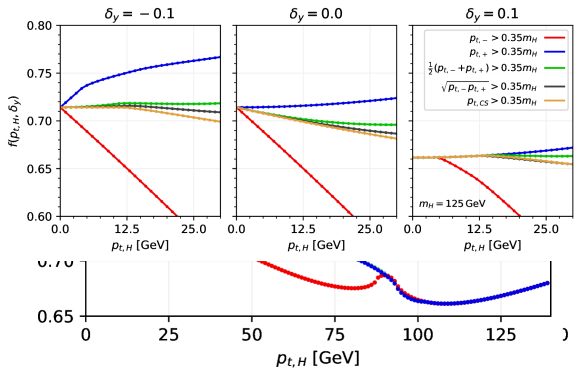
Figure 4: Comparison of the $p_{t,\text{\sc h}}$-dependent acceptances for the sum, product and staggered cuts. For the staggered cuts, $p_{t,y_{+}}$ corresponds to the transverse momentum of the photon at higher rapidity. As in Fig. 2, the points corresponds to Monte Carlo evaluations of the acceptances. Lines use series expansions to fourth order and bands (where visible) show the size of the fourth order term.

The acceptances for the three sets of “quadratic” cuts are shown in Fig. 4, and can be compared to the acceptances for standard symmetric and asymmetric cuts (with linear $p_{t,\text{\sc h}}$ dependence) in Fig. 2. The vertical scales have the same extent, but are shifted by $0.1$. All three quadratic cuts lead to considerably flatter $p_{t,\text{\sc h}}$ dependence, as was expected, and represent good, simple alternatives to standard symmetric and asymmetric cuts. One clearly sees the transition to linear $p_{t,\text{\sc h}}$ dependence for $p_{t,\text{\sc h}}\gtrsim 2\Delta$ in the case of the sum and product cuts and for $p_{t,\text{\sc h}}>\Delta$ for the staggered cuts.

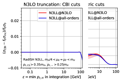
Figure 5: The N3LL resummed result and its N3LO truncation, for sum cuts (left) and product cuts (right), as a function of $\epsilon$, the minimum $p_{t,\text{\sc h}}$ in Eq. (23). Note the different scale relative to Fig. 3.

The perturbative convergence of the acceptance with sum and product cuts is illustrated with the following results for the perturbative series, first for the sum cuts,

$$\frac{\sigma_{\text{sum}}-f_{0}\sigma_{\text{inc}}}{\sigma_{0}f_{0}} \simeq 0.013_{\alpha_{s}}-0.007_{\alpha_{s}^{2}}+0.005_{\alpha_{s}^{3}}-0.004_{\alpha_{s}^{4}}+0.004_{\alpha_{s}^{5}}+\ldots \simeq 0.009\;\; @\text{DL},$$

$$\simeq 0.013_{\alpha_{s}}-0.005_{\alpha_{s}^{2}}+0.001_{\alpha_{s}^{3}}-0.001_{\alpha_{s}^{4}}+0.000_{\alpha_{s}^{5}}+\ldots \simeq 0.010\;\; @\text{LL},$$

$$\simeq 0.016_{\alpha_{s}}+0.007_{\alpha_{s}^{2}}-0.004_{\alpha_{s}^{3}}+\ldots \simeq 0.019\;\; @\text{NNLL},$$

$$\simeq 0.016_{\alpha_{s}}+0.007_{\alpha_{s}^{2}}-0.001_{\alpha_{s}^{3}}+\ldots \simeq 0.021\;\; @\text{N3LL},$$

and next for product cuts,

$$\frac{\sigma_{\text{prod}}-f_{0}\sigma_{\text{inc}}}{\sigma_{0}f_{0}} \simeq 0.005_{\alpha_{s}}-0.002_{\alpha_{s}^{2}}+0.002_{\alpha_{s}^{3}}-0.001_{\alpha_{s}^{4}}+0.001_{\alpha_{s}^{5}}+\ldots \simeq 0.003\;\; @\text{DL},$$

$$\simeq 0.005_{\alpha_{s}}-0.002_{\alpha_{s}^{2}}+0.000_{\alpha_{s}^{3}}-0.000_{\alpha_{s}^{4}}+0.000_{\alpha_{s}^{5}}+\ldots \simeq 0.003\;\; @\text{LL},$$

$$\simeq 0.005_{\alpha_{s}}+0.002_{\alpha_{s}^{2}}-0.001_{\alpha_{s}^{3}}+\ldots \simeq 0.005\;\; @\text{NNLL},$$

$$\simeq 0.005_{\alpha_{s}}+0.002_{\alpha_{s}^{2}}-0.001_{\alpha_{s}^{3}}+\ldots \simeq 0.006\;\; @\text{N3LL}.$$

The improvement in convergence relative to the corresponding results for asymmetric cuts, Eq. (2.3) is striking.

Fig. 5, which is to be compared to its analogue for asymmetric cuts, i.e. Fig. 3, shows the sensitivity to the infrared cutoff in Eq. (23), as well as the impact of scale variation. N3LO (from N3LL) and the full N3LL resummation now agree well and the N3LO result is much less sensitive to the minimum $p_{t,\text{\sc h}}$ in the integration, converging at a few GeV, rather than at MeV scales for asymmetric cuts. These are precisely the features that we had anticipated in the introduction to this section. Note also that the residual scale uncertainty is now essentially negligible (at least by today’s standards for Higgs physics), and that the overall size of the fiducial acceptance correction is much smaller than for asymmetric cuts. Note that in Eqs. (3.4) and (3.4), at N3LL the coefficient of the $\alpha_{s}^{2}$ term is now positive, whereas it is negative at DL and LL. The most likely explanation for the change of sign is that it is related to the interplay between the acceptance cuts and the large (positive) NLO $K$-factor for Higgs production.

Of the three quadratic cuts discussed so far, overall the best choice appears to be the product cuts, for several reasons:

1. The coefficient of the quadratic dependence is small (though staggered cuts give a smaller coefficient for $2p_{t\text{cut}}/m_{\text{\sc h}}<1/\sqrt{2}$).

2. The transition point to quasi-linear $p_{t,\text{\sc h}}$ dependence, at $p_{t,\text{\sc h}}\simeq 2\Delta$, is the highest of the three (sum cuts transition at a similar, though slightly lower value of $p_{t,\text{\sc h}}$). Having a high transition point is of value because it means that the substantial $p_{t,\text{\sc h}}$ dependence occurs in a region where the perturbative prediction for the $p_{t,\text{\sc h}}$ spectrum is more likely to be reliable, providing confidence in the use of pure fixed-order perturbation theory to calculate acceptances.

3. The acceptance remains high at the highest values of $p_{t,\text{\sc h}}$ shown in Fig. 4, significantly higher than with staggered cuts, albeit slightly lower than with sum cuts.

One context in which one might prefer staggered cuts (or a cut just on the charged lepton Sirunyan:2020oum ) is for the study of $W$ bosons, where significantly different experimental resolutions and background contributions for neutrinos versus charged leptons may favour the application of distinct cuts. One may also wish to use staggered cuts for $Z/\gamma^{*}$ decays in situations where the $Z/\gamma^{*}$ decays are effectively being used as a calibration for the $W$’s (the cuts on the $Z$ decay products should then perhaps then be scaled by a factor $m_{Z}/m_{W}$ relative to the $W$ cuts). For $W$ and $Z$ production, having the quadratic regime extend only to $p_{t}=\Delta$ rather than $p_{t}\simeq 2\Delta$ should be less of an issue than in Higgs production: the presence of a $C_{F}=4/3$ versus $C_{A}=3$ coefficient in the $p_{t}$ resummation means that the region of good perturbative control at fixed order will extend to lower $p_{t}$ than for Higgs production. Further discussion about $Z$ production is to be found in section 6.

Our final remarks concern the values of the thresholds. If one adopts product or sum cuts with the same values for the thresholds as used currently for asymmetric cuts (e.g. $0.35m_{\text{\sc h}}$ and $0.25m_{\text{\sc h}}$) any event that passes existing asymmetric cuts will also pass the sum and product cuts. Thus the events collected with asymmetric cuts could, in principle, be straightforwardly reanalysed with the sum or product cuts. One should be aware that because the resummed fiducial correction is smaller with sum and product cuts than with the asymmetric cuts (cf. Eqs. (3.4) and (3.4) versus Eq. (2.3)), there will be a slight loss in Higgs statistics with sum or product cuts (taking into account a Higgs $K$-factor of about $3$ relative to the Born cross section, the numbers suggest roughly $3{-}4\%$, with the background also being reduced). However, in future data collection (and depending on triggers, perhaps also with already recorded data), there may be freedom to adjust cut thresholds. For example, lowering the $0.35m_{\text{\sc h}}$ threshold to $0.30m_{\text{\sc h}}$ (while retaining a fixed $p_{t,-}$ threshold of $0.25m_{\text{\sc h}}$) would still leave a significant region where the quadratic $p_{t,\text{\sc h}}$ dependence holds (up to $p_{t,\text{\sc h}}\simeq 12.5\;\mathrm{GeV}$), while raising the acceptance by more than enough to compensate for the loss in switching from asymmetric to product cuts. Optimisation of the choice of thresholds probably needs experimental input, e.g. as concerns the behaviour of the continuum di-photon background (including its fake-photon contribution), as well as theoretical input, e.g. in terms of verifying the perturbative behaviour of each given set of cuts.

3.5 Boost-invariant cuts via Collins-Soper decay transverse momentum

The quadratic cuts that we have seen so far are already a significant improvement on widely used symmetric and asymmetric cuts and Fig. 5 suggests that any residual non-convergence issues of the perturbative series are not likely to be of imminent practical importance. Still, the perturbative series in Eq. (26) reaches a breakdown in convergence earlier than one might hope for, even if the coefficients of the breakdown are small. Furthermore the effective power scaling of the minimal term of the perturbative series in the DL approximation, $(\Lambda/Q)^{23/36}$ (Eq. (14)), is not entirely reassuring, even if subleading logarithmic effects are likely to modify the power.

In this subsection we start our investigation of cuts for which the acceptance is entirely independent of $p_{t,\text{\sc h}}$ at small values of $p_{t,\text{\sc h}}$ (with the remainder of our analysis to be given in section 5, after we have considered the issue of rapidity cuts). We will work within the constraint that a direct cut of $p_{t,\text{cut}}-\Delta$ on the $p_{t}$ on the softer of the two photons is experimentally unavoidable. Additionally, we will aim to maintain the same $p_{t,\text{\sc h}}=0$ acceptance as for the asymmetric, product and sum cuts.

At $p_{t,\text{\sc h}}=0$ a cut on $p_{t,\pm}$ is equivalent to a cut on $\sin\theta$ in the Collins-Soper parametrisation of the decay phase space in Eq. (2). Our core idea here is to cut on $\sin\theta$ as defined in that parametrisation also for non-zero $p_{t,\text{\sc h}}$. In practice we express this condition by introducing a “Collins-Soper” decay transverse momentum in terms of the kinematics of the two decay products

$$\vec{p}_{t,\text{\sc cs}}=\frac{1}{2}\left[\vec{\delta}_{t}+\frac{\vec{p}_{t,12}.\vec{\delta}_{t}}{p_{t,12}^{2}}\left(\frac{m_{12}}{\sqrt{\smash[b]{m_{12}^{2}+p_{t,12}^{2}}}}-1\right)\vec{p}_{t,12}\right]\,,\qquad\vec{\delta}_{t}=\vec{p}_{t,1}-\vec{p}_{t,2}\,,$$ (39)

where $\vec{p}_{t}$ is the (two-dimensional) vector transverse component of a momentum $p$ and the dot product is a two-dimensional scalar product. It is irrelevant which of the decay products is labelled $1$ and $2$. We have written the definition in terms $m_{12}$, the invariant mass of the two-body system and $\vec{p}_{t,12}$, the net transverse momentum of the two-body system, which in the Higgs decay case are simply $m_{\text{\sc h}}$ and ${\vec{p}}_{t,\text{\sc h}}$. At $p_{t,12}\equiv p_{t,\text{\sc h}}=0$, the second term in the square brackets vanishes and since the two decay products are back to back, $p_{t,\text{\sc cs}}=p_{t,1}=p_{t,2}$. For general $p_{t,\text{\sc h}}$ it is straightforward to verify that Eq. (39) yields $2p_{t,\text{\sc cs}}/m_{12}\equiv\sin\theta$. Our cuts are then $p_{t,\text{\sc cs}}>p_{t,\text{cut}}$ and $p_{t,-}>p_{t,\text{cut}}-\Delta$.

For values of $p_{t,\text{\sc h}}$ that are not too large,

$$p_{t,\text{\sc h}}<p_{t,\text{\sc h}}^{\text{\sc cs}\text{-threshold}} =\frac{2m_{\text{\sc h}}\left(p_{t,\text{cut}}\sqrt{m_{\text{\sc h}}^{2}+4\Delta(\Delta-2p_{t,\text{cut}})}+m_{\text{\sc h}}(\Delta-p_{t,\text{cut}})\right)}{m_{\text{\sc h}}^{2}-4p_{t,\text{cut}}^{2}},$$ (40a)

$$=2\Delta+\frac{4p_{t,\text{cut}}\Delta^{2}}{m_{\text{\sc h}}^{2}}+\mathcal{O}_{3}\,,$$ (40b)

the acceptance is simply $f(p_{t,\text{\sc h}})=f_{0}$. Including the region beyond the transition at first order in $p_{t,\text{\sc h}}/m_{\text{\sc h}}$ we have

$$f^{\text{\text{\sc cs}}}(p_{t,\text{\sc h}})=f_{0}-\frac{4p_{t,\text{cut}}}{\pi m_{\text{\sc h}}f_{0}}\frac{\chi(p_{t,\text{\sc h}},2\Delta+\mathcal{O}_{2})}{m_{\text{\sc h}}}\left(1+\mathcal{O}_{2}\right),$$ (41)

with, once again, the usual transition beyond $p_{t,\text{\sc h}}\simeq 2\Delta$.

Figure 6: Comparison of the $p_{t,\text{\sc h}}$-dependent acceptance of the Collins-Soper $p_{t,\text{\sc cs}}$ cut with that of the product cuts (both sets of cuts also include the constraint $p_{t,-}>0.25m_{\text{\sc h}}$), as well as a cut just on the softer photon $p_{t}$ (i.e. a symmetric cut). As in Figs. 2 and 4, the points corresponds to Monte Carlo evaluations of the acceptances. Note the different scale used here.

Fig. 6 compares the $p_{t,\text{\sc cs}}$ cut acceptance with that of the product cut (both additionally include the requirement $p_{t,-}>0.25m_{\text{\sc h}}$). Up to $p_{t,\text{\sc h}}\simeq 2\Delta=0.2m_{\text{\sc h}}$, the $p_{t,\text{\sc cs}}$ cut acceptance is independent of $p_{t,\text{\sc h}}$, as desired. However at larger $p_{t,\text{\sc h}}$ values, it has a considerably lower acceptance than the product cut. This is less than ideal phenomenologically, because in that region events are relatively rare and one may wish to maximise acceptance within the constraints posed by the photon reconstruction requirement, $p_{t,-}>0.25m_{\text{\sc h}}$ (shown in green on the plot). For $p_{t,\text{\sc h}}\gtrsim 2\Delta$, the product cut comes much closer to achieving this. It turns out that it is possible to design techniques to recover the high-$p_{t,\text{\sc h}}$ acceptance that is lost with the $p_{t,\text{\sc cs}}$ cuts. The approach that we take will be useful not just for addressing $p_{t,\text{\sc h}}$-acceptance dependence with hardness cuts, but also with rapidity cuts. Accordingly we introduce it in section 5, after our discussion of rapidity cuts and their interplay with hardness cuts.

One feature that the reader may have noticed is that the coefficient of the $\chi$ function is identical for all of the cuts in this section, yet even those that share transitions at $p_{t,\text{\sc h}}\simeq 2\Delta$ show rather different behaviours beyond that point (for example product and $p_{t,\text{\sc cs}}$ cuts in Fig. 6). Recall, however, that the $\chi$ function in Eqs. (31,34,41) is accompanied by higher powers of $p_{t,\text{\sc h}}/m_{\text{\sc h}}$ and $\Delta/m_{\text{\sc h}}$, which we have not explicitly written down analytically (but which are included in the lines in Figs. 4 and 6). It is those higher-power terms that are responsible for the different behaviours beyond $2\Delta$.

4 Rapidity cuts

Our focus so far has been on hardness cuts, which are essential for eliminating the high event rates associated with low-$p_{t}$ photons, leptons, etc. and for avoiding momentum regions where objects may be poorly measured. Real experiments also have limitations on the range of (pseudo)rapidities over which they can measure particles, which also induce $p_{t,\text{\sc h}}$ dependence of the acceptance.

Since we are working with an assumption of massless (or quasi-massless) decay products, rapidities and pseudorapidities are identical. For brevity, here, we just use the term rapidity.

The key results that we will obtain in this section are that a single rapidity cut leads to quadratic acceptance, Eq. (43); that a linear $p_{t,\text{\sc h}}$ dependence reappears when the Higgs rapidity is midway between two photon rapidity cuts; and, for a rapidity cut in combination with quadratic (or better) hardness cuts, linear dependence arises also at the Higgs rapidity where the photon hardness and rapidity cuts are equivalent ($\delta_{y}=0$ in Eq. (53)). Those linear behaviours are eliminated once one takes finite rapidity bins around the critical rapidity points, though the residual quadratic behaviours for the corresponding bins have a coefficient of $p_{t,\text{\sc h}}^{2}$ that scales as the inverse bin width, suggesting that the bins around those points should be reasonably wide.

On a first pass, some readers may wish to skip the technical details that we provide in this section and go straight to the practical example in section 4.4.

4.1 A single rapidity cut

Suppose that we have a Higgs boson at rapidity $y_{\text{\sc h}}=0$, decaying to positive and negative-rapidity photons, $\gamma_{y_{+}}$ and $\gamma_{y_{-}}$, with rapidities $y_{y_{+}}$ and $y_{y_{-}}$ respectively. We start our study of rapidity cuts by examining what happens with a single rapidity cut, $y_{y_{+}}<y_{\text{cut}}$. We will again follow the methods of section 2, in particular keeping the parametrisation Eq. (2). The one critical difference is that while we will maintain $0\leq\theta\leq\pi/2$, we will allow the full azimuthal range $-\pi\leq\phi\leq\pi$, because that full range yields $y_{+}\geq 0$ and $y_{-}\leq 0$. For a given value of $\phi$, the rapidity cut can straightforwardly be translated to a limit on $\cos\theta$,

$$\cos\theta<\tanh y_{\text{cut}}\left[1+\frac{\cos\phi}{\cosh y_{\text{cut}}}\cdot\frac{p_{t,\text{\sc h}}}{m_{\text{\sc h}}}+\frac{1}{2}\left(\operatorname{csch}^{2}y_{\text{cut}}-\cos 2\phi\right)\tanh^{2}y_{\text{cut}}\cdot\frac{p_{t,\text{\sc h}}^{2}}{m_{\text{\sc h}}^{2}}+\mathcal{O}_{3}\right].$$ (42)

Integrating over the full $\phi$ range, the term linear in $p_{t,\text{\sc h}}$ averages to zero and we are left with an acceptance with a quadratic dependence on $p_{t,\text{\sc h}}$, which for general Higgs boson rapidity $y_{\text{\sc h}}$ reads

$$f^{<y_{\text{cut}}}(p_{t,\text{\sc h}},y_{\text{\sc h}})=\Theta(y_{\text{cut}}-y_{\text{\sc h}})\tanh(y_{\text{cut}}-y_{\text{\sc h}})\left[1+\frac{1}{2}\operatorname{sech}^{2}(y_{\text{cut}}-y_{\text{\sc h}})\cdot\frac{p_{t,\text{\sc h}}^{2}}{m_{\text{\sc h}}^{2}}+\mathcal{O}_{4}\right].$$ (43)

The mechanism that causes the linear term to vanish is fundamentally different from that in the sum and product $p_{t}$ cuts in section 3: there the product and sum kinematic variables were free of any linear $p_{t,\text{\sc h}}$ term, independently of $\phi$; here the linear term is present for almost all $\phi$ values and it is only after the $\phi$ integral that it drops out, as for the staggered cuts of section 3.3. Anything that breaks the $\phi\to\pi+\phi$ cancellation will result in the linear dependence reappearing.

4.2 Two rapidity cuts

To understand the behaviour of the acceptance in situations with two rapidity cuts, we situate the Higgs boson at rapidity $y_{\text{\sc h}}$ and apply a requirement that both decay photons should satisfy $|y|<y_{\text{cut}}$. Our first observation is that if $y_{\text{\sc h}}=0$, we have Eq. (42) for the positive-rapidity photon and a similar relation for the negative-rapidity photon with the replacement $\phi\to\pi+\phi$, i.e. a change of sign for the $\cos\phi$ term. Both conditions must be satisfied simultaneously: in the region $|\phi|<\pi/2$ it is the condition on the negative-rapidity photon that will be more constraining, while for $\pi/2<|\phi|<\pi$ it is the condition on the positive-rapidity photon that will be more constraining. The acceptance can be obtained by integrating just the condition for the negative-rapidity photon in the region $|\phi|<\pi/2$, giving

$$f^{\lessgtr\pm y_{\text{cut}}}(p_{t,\text{\sc h}},y_{\text{\sc h}}=0)=\tanh y_{\text{cut}}\left[1-\frac{2}{\pi}\operatorname{sech}y_{\text{cut}}\cdot\frac{p_{t,\text{\sc h}}}{m_{\text{\sc h}}}+\frac{1}{2}\operatorname{sech}^{2}y_{\text{cut}}\cdot\frac{p_{t,\text{\sc h}}^{2}}{m_{\text{\sc h}}^{2}}+\mathcal{O}_{3}\right].$$ (44)

The presence of a linear $p_{t,\text{\sc h}}$ term is a consequence of the loss of the azimuthal cancellation between $\phi$ and $\phi+\pi$. The linear $p_{t,\text{\sc h}}$ dependence extends down to $p_{t,\text{\sc h}}=0$ only if the Higgs boson is exactly mid-way between the rapidity cuts. If we retain the cuts at $\pm y_{\text{cut}}$, but give a small non-zero rapidity to the Higgs boson, we obtain

$$f^{\lessgtr\pm y_{\text{cut}}}(p_{t,\text{\sc h}},y_{\text{\sc h}})=f^{y_{\text{cut}}}(p_{t,\text{\sc h}},|y_{\text{\sc h}}|)-\frac{2\tanh y_{\text{cut}}}{\pi m_{\text{\sc h}}\cosh y_{\text{cut}}}\,\chi\!\left(p_{t,\text{\sc h}},\frac{|y_{\text{\sc h}}|\,m_{\text{\sc h}}}{\sinh y_{\text{cut}}}+\mathcal{O}_{2}\right)(1+\mathcal{O}_{2})\,,$$ (45)

i.e. we retain the quadratic behaviour of Eq. (43) up to $p_{t,\text{\sc h}}=|y_{\text{\sc h}}|\,m_{\text{\sc h}}/\sinh y_{\text{cut}}$ and then observe a transition with the usual $\chi$ function.

In practice, experimental results that are differential in $y_{\text{\sc h}}$ are presented in finite bins of $y_{\text{\sc h}}$. The rapidity bin that is most critical is the one that contains a Higgs rapidity midway between two photon rapidity cuts (i.e. the $y_{\text{\sc h}}=0$ point in our simple example here). If we consider a rapidity bin of half-width $\delta$ that covers the region $|y_{\text{\sc h}}|<\delta$, assuming that we can ignore the dependence of the Higgs differential cross section on $y_{\text{\sc h}}$, we obtain

$$\left\langle f^{\lessgtr\pm y_{\text{cut}}}(p_{t,\text{\sc h}},y_{\text{\sc h}})\right\rangle_{|y_{\text{\sc h}}|<\delta}=\frac{1}{\delta}\int_{0}^{\delta}f^{y_{\text{cut}}}(p_{t,\text{\sc h}},|y_{\text{\sc h}}|)dy_{\text{\sc h}}\,+\\ -\frac{1}{\delta}\cdot\frac{2\tanh y_{\text{cut}}}{\pi m_{\text{\sc h}}\cosh y_{\text{cut}}}\int_{0}^{\min\left(\delta,\frac{p_{t,\text{\sc h}}\sinh y_{\text{cut}}}{m_{\text{\sc h}}}\right)}\chi\!\left(p_{t,\text{\sc h}},\frac{y_{\text{\sc h}}\,m_{\text{\sc h}}}{\sinh y_{\text{cut}}}\right)dy_{\text{\sc h}}+\mathcal{O}_{2}\,.$$ (46)

At this point, it is useful to define

$$\bar{\chi}(x,\delta)=\int_{0}^{\delta}d\delta_{y}\,\chi(x,\delta_{y})\,,$$ (47)

which is zero for negative values of $\delta$ and otherwise evaluates to

$$\bar{\chi}(x,\delta)\equiv\left\{\begin{array}[]{lll}\frac{\pi}{8}x^{2}\,,&&x\leq\delta\,,\\ \frac{3\delta}{4}\sqrt{x^{2}-\delta^{2}}+\frac{x^{2}}{4}\left(2\arctan\frac{\delta}{\sqrt{x^{2}-\delta^{2}}}-\arcsin\frac{\delta}{x}\right)-\frac{\delta^{2}}{2}\arccos\frac{\delta}{x}\,,&&x>\delta\,.\end{array}\right.$$ (48)

The critical features to observe are the quadratic behaviour in $x$ for small values of $x$, while for $x\gg\delta$, $\bar{\chi}(x,\delta)$ is approximately equal to $\delta\cdot x$. The result for Eq. (46) can now be written

$$\left\langle f^{\lessgtr\pm y_{\text{cut}}}(p_{t,\text{\sc h}},y_{\text{\sc h}})\right\rangle_{|y_{\text{\sc h}}|<\delta}=\tanh y_{\text{cut}}-\left(\frac{\delta}{2\cosh^{2}y_{\text{cut}}}+\frac{2\tanh^{2}y_{\text{cut}}}{\delta\cdot\pi m_{\text{\sc h}}^{2}}\bar{\chi}\!\left(p_{t,\text{\sc h}},\frac{y_{\text{\sc h}}\,m_{\text{\sc h}}}{\sinh y_{\text{cut}}}\right)\right)+\mathcal{O}_{2}\,,$$ (49)

where we count powers of $p_{t,\text{\sc h}}/m_{\text{\sc h}}$ and $\delta$ on the same footing from the point of view of the series expansion. When $p_{t,\text{\sc h}}<\delta\cdot m_{\text{\sc h}}/\sinh y_{\text{cut}}$, this becomes

$$\left\langle f^{\lessgtr\pm y_{\text{cut}}}(p_{t,\text{\sc h}},y_{\text{\sc h}})\right\rangle_{|y_{\text{\sc h}}|<\delta}=\tanh y_{\text{cut}}-\left(\frac{\delta}{2\cosh^{2}y_{\text{cut}}}+\frac{\tanh^{2}y_{\text{cut}}}{4\delta}\cdot\frac{p_{t,\text{\sc h}}^{2}}{m_{\text{\sc h}}^{2}}\right)+\mathcal{O}_{2}\,.$$ (50)

We see that for small $p_{t,\text{\sc h}}$, the linear $p_{t,\text{\sc h}}$ dependence that was present in Eq. (44) vanishes, to be replaced by a quadratic dependence on $p_{t,\text{\sc h}}$ that is enhanced by $1/\delta$. This leads to an important practical consideration: in the vicinity of a rapidity value that is midway between two rapidity cuts, one should ensure that the rapidity bin has a half-width $\delta$ that is not too small, so as to ensure that the coefficient of the quadratic $p_{t,\text{\sc h}}^{2}/m_{\text{\sc h}}^{2}$ dependence, $\tanh^{2}(y_{\text{cut}}-y_{\text{\sc h}})/4\delta$, is not too large.

Our final comments here concern other combinations of rapidity cuts, which are relevant when considering rapidity ranges with excluded bands, e.g. $|\eta_{\gamma}|<2.37$ but excluding $1.37<|\eta_{\gamma}|<1.52$ for ATLAS Aaboud:2018xdt and similar cuts for CMS Sirunyan:2018kta . Considering a pair of cuts at a time, there are two generic situations beyond that discussed above. One can be cast as a requirement $y_{y_{-}}<-y_{\text{cut}}$ and $y_{y_{+}}<y_{\text{cut}}$, in which case the result is given by

$$f^{<\pm y_{\text{cut}}}(p_{t,\text{\sc h}},y_{\text{\sc h}})=f^{<+y_{\text{cut}}}(p_{t,\text{\sc h}},y_{\text{\sc h}})-f^{\lessgtr\pm y_{\text{cut}}}(p_{t,\text{\sc h}},y_{\text{\sc h}})\,,$$ (51)

while the other can be cast as the requirement $y_{y_{-}}<-y_{\text{cut}}$ and $y_{y_{+}}>y_{\text{cut}}$, yielding

$$f^{\gtrless\pm y_{\text{cut}}}(p_{t,\text{\sc h}},y_{\text{\sc h}})=1-\left(f^{<+y_{\text{cut}}}(p_{t,\text{\sc h}},y_{\text{\sc h}})+f^{>-y_{\text{cut}}}(p_{t,\text{\sc h}},y_{\text{\sc h}})-f^{\lessgtr\pm y_{\text{cut}}}(p_{t,\text{\sc h}},y_{\text{\sc h}})\right).$$ (52)

From these results, one sees that the midpoint between any pair of rapidity cuts will involve the same kinds of structures.

4.3 Combination of rapidity and $p_{t}$ cuts

The final situation that needs to be considered is that when the rapidity and transverse momentum cuts for the decay products cover similar phase space. In terms of our understanding of the small-$p_{t,\text{\sc h}}$ behaviour of the acceptance, the relevant region is when the rapidity and leading photon $p_{t}$ cut lead to similar acceptances for $p_{t,\text{\sc h}}=0$, i.e. when

$$\delta_{y}\equiv y_{\text{\sc h}}-\left(y_{\text{cut}}-\operatorname{arccosh}\frac{m_{\text{\sc h}}}{2p_{t,\text{cut}}}\right)\ll 1\,,$$ (53)

working in the regime $y_{\text{\sc h}}<y_{\text{cut}}$ and where the rapidity cut vetoes photons with $y>y_{\text{cut}}$. Many of our hardness cuts involve two scales: a main hardness cut, $p_{t,\text{cut}}$, and a subsidiary condition on the softer decay product, $p_{t,-}>p_{t,\text{cut}}-\Delta$. To simplify our analysis here, we will work with the assumption that we can neglect that softer cut, or correspondingly, $\delta_{y}\ll\Delta/m_{\text{\sc h}}$.

To keep our results compact it will be helpful to define a “base” result for a hardness cut H

$$f_{\text{base}}^{\text{H}}(p_{t,\text{\sc h}},\delta_{y})=\left\{\begin{array}[]{lll}f^{\text{H}}(p_{t,\text{\sc h}})&&\delta_{y}<0\,,\\ f^{<y_{\text{cut}}}(p_{t,\text{\sc h}},\delta_{y})&&\delta_{y}>0\,,\end{array}\right.$$ (54)

which selects the correct small $p_{t,\text{\sc h}}$ behaviour for the efficiency depending on whether $\delta_{y}<0$ (the hardness cut is the only relevant one) or $\delta_{y}>0$ (the rapidity cut is the only relevant one).

It will be convenient to use the shorthands

$$s_{0}=\frac{2p_{t,\text{cut}}}{m_{\text{\sc h}}}\,,\qquad f_{0}=\sqrt{1-s_{0}^{2}}\,.$$ (55)

For a symmetric $p_{t}$ cut we obtain

$$f^{\text{sym}}(p_{t,\text{\sc h}},\delta_{y})\simeq f_{\text{base}}^{\text{sym}}(p_{t,\text{\sc h}},\delta_{y})-\frac{\left(1+f_{0}^{2}\right)s_{0}}{\pi f_{0}}\chi\!\left(\frac{p_{t,\text{\sc h}}}{m_{\text{\sc h}}},\frac{f_{0}s_{0}\delta_{y}}{1+f_{0}^{2}}\right)-\frac{s_{0}^{3}}{\pi f_{0}}\chi\!\left(\frac{p_{t,\text{\sc h}}}{m_{\text{\sc h}}},\frac{f_{0}\delta_{y}}{s_{0}}\right).$$ (56)

Throughout this section, when we write $\simeq$, it means that we drop $\mathcal{O}_{2}$ terms in the structure associated with the $\chi$ functions, both for the shape of the function and the location of its turn-on. Recall that our definition of the $\chi$ function, Eq. (19), includes a $\Theta$ function such that $\chi$ is non-zero only when the first argument (which is always positive) is larger than the second one and the second one is positive. Thus Eq. (56) shows that the combination of a $p_{t}$ and rapidity cut induces changes in the acceptance relative to Eq. (54) only when $\delta_{y}>0$. The presence of two $\chi$ functions tells us that there are two values of $p_{t,\text{\sc h}}$ at which there will be a transition in the $p_{t,\text{\sc h}}$ dependence. They are associated with the intersections of the $p_{t}$ and rapidity cuts at $\phi=\pi$ and $\phi=0$ respectively.

The resulting acceptance is shown as the red lines ($p_{t,-}>0.35m_{\text{\sc h}}$) in Fig. 7, with each panel corresponding to a different value of $\delta y$. With the cuts shown, $s_{0}=0.7$ and $f_{0}\simeq 0.714$ are almost equal. For $\delta_{y}\leq 0$, the rapidity cut has no impact over the range shown, while for $\delta_{y}=0.1$, one sees a first kink at $p_{t,\text{\sc h}}\simeq 0.33\,\delta_{y}m_{\text{\sc h}}\simeq 4.1\;\mathrm{GeV}$ and a second, weaker kink at $p_{t,\text{\sc h}}\simeq 1.02\,\delta_{y}m_{\text{\sc h}}\simeq 12.8\;\mathrm{GeV}$. Note that for $p_{t,\text{\sc h}}$ significantly larger than the position of the kinks, the normalisations of the $\chi$-terms in Eq. (56) add up to give $-\frac{2s_{0}}{\pi f_{0}}$ multiplying $p_{t,\text{\sc h}}/m_{\text{\sc h}}$, which is precisely $f_{1}^{\text{sym}}$ in Eq. (8).

Figure 7: Acceptance for a combination of a hardness cut (as specified in the legend) and a single photon rapidity cut. The quantity $\delta_{y}$ is defined in Eq. (53). For the hardness cuts that would normally have two separate hardness scales (i.e. all but the symmetric cut) we have set the lower cut to zero, so as to concentrate on the interplay between the harder cut and rapidity cut, as is appropriate in the region $\delta_{y}\ll\Delta/m_{\text{\sc h}}$ that we set out to study. The points, lines and bands follow the usual convention of Fig. 2.

For a standard asymmetric cut, which in our limit of $\delta_{y}\ll\Delta/m_{\text{\sc h}}$ is equivalent to a cut on the $p_{t}$ just of the harder photon, we obtain

$$f^{\text{asym}}(p_{t,\text{\sc h}},\delta_{y})\simeq f_{\text{base}}^{\text{asym}}(p_{t,\text{\sc h}},\delta_{y})-\frac{\left(1+f_{0}^{2}\right)s_{0}}{\pi f_{0}}\chi\left(\frac{p_{t,\text{\sc h}}}{m_{\text{\sc h}}},-\frac{f_{0}s_{0}\delta_{y}}{f_{0}^{2}+1}\right)-\frac{s_{0}^{3}}{\pi f_{0}}\chi\left(\frac{p_{t,\text{\sc h}}}{m_{\text{\sc h}}},-\frac{f_{0}\delta_{y}}{s_{0}}\right).$$ (57)

Now the two transitions are present only for negative values of $\delta_{y}$. The resulting acceptance is again shown in Fig. 7, as the blue lines ($p_{t,+}>0.35m_{\text{\sc h}}$). For $\delta_{y}\geq 0$, the result corresponds to just the rapidity cut, i.e. quadratic $p_{t,\text{\sc h}}$ dependence, while for $\delta_{y}=-0.1$ one sees a clear first kink around $0.33|\delta_{y}|m_{\text{\sc h}}$ and a weaker second kink around $1.02|\delta_{y}|m_{\text{\sc h}}$. The normalisation is such that sufficiently far beyond the second kink (but before $p_{t,\text{\sc h}}=\Delta$ asymmetric cut transition would be reached), the positive linear $p_{t,\text{\sc h}}$ dependence from $f_{1}^{\text{asym}}$ of Eq. (15) is cancelled out.

Finally, using H to denote any of the sum, product and Collins–Soper boost-invariant hardness cuts, we have

$$f^{\text{H}}(p_{t,\text{\sc h}},\delta_{y})\simeq f^{\text{H}}_{\text{base}}(p_{t,\text{\sc h}},\delta_{y})-\frac{f_{0}s_{0}}{\pi}\chi\left(\frac{p_{t,\text{\sc h}}}{m_{\text{\sc h}}},\frac{s_{0}|\delta_{y}|}{f_{0}}\right),$$ (58)

where there is just a single transition, which is present for both positive and negative values of $\delta_{y}$. Again, the results are shown in Fig. 7. For $\delta_{y}=-0.1$, one sees the three quadratic (or flat) low-$p_{t,\text{\sc h}}$ acceptances for each of the sum, product or $p_{t,\text{\sc cs}}$ cuts, with a kink at $p_{t,\text{\sc h}}\simeq 0.98|\delta_{y}|m_{\text{\sc h}}\simeq 12.3\;\mathrm{GeV}$, transitioning to a linear $p_{t,\text{\sc h}}$ dependence. For $\delta_{y}=0$ that linear $p_{t,\text{\sc h}}$ dependence is present from $p_{t,\text{\sc h}}=0$ and the small differences between the three cuts reflect their differing quadratic terms. For $\delta_{y}=0.1$, we initially have the quadratic $p_{t,\text{\sc h}}$ dependence that is characteristic of just the rapidity cut, and following the kink a hint of linear dependence arising. Note that the coefficient of the linear dependence, $f_{0}s_{0}/\pi$, is about four times smaller than that for the symmetric or asymmetric cuts.

At first sight, it is concerning that hardness cuts that led to quadratic or flat $p_{t,\text{\sc h}}$ dependence, when combined with a rapidity cut, now reacquire linear dependence at $\delta_{y}=0$. However, as with the discussion of pairs of rapidity cuts in section 4.2, the question that is ultimately relevant for practical perturbative calculations is not what happens at a given point in rapidity, but what happens after integration over a given rapidity bin. For $H$ denoting any of the sum, product, and $p_{t,\text{\sc cs}}$ cuts, considering a bin of half width $\delta$ centred at $\delta_{y}=0$, we have

$$\left\langle f^{H,y_{+}<y_{\text{cut}}}(p_{t,\text{\sc h}},\delta_{y})\right\rangle_{|\delta_{y}|<\delta}\simeq f^{H}(p_{t,\text{\sc h}})-\left(\frac{s_{0}^{2}}{4}\delta+\frac{f_{0}^{2}}{\pi\delta}\bar{\chi}\left(\frac{p_{t,\text{\sc h}}}{m_{\text{\sc h}}},\frac{s_{0}\delta}{f_{0}}\right)\right),$$ (59)

with $\bar{\chi}$ as given in Eq. (48). For $p_{t,\text{\sc h}}<\frac{s_{0}\delta}{f_{0}}m_{\text{\sc h}}$  the result reduces to

$$\left\langle f^{H,y_{+}<y_{\text{cut}}}(p_{t,\text{\sc h}},\delta_{y})\right\rangle_{|\delta_{y}|<\delta}\simeq f^{H}(p_{t,\text{\sc h}})-\left(\frac{s_{0}^{2}}{4}\delta+\frac{f_{0}^{2}}{8\delta}\frac{p_{t,\text{\sc h}}^{2}}{m_{\text{\sc h}}^{2}}\right).$$ (60)

As with the rapidity integral for the pair of rapidity cuts, we see quadratic $p_{t,\text{\sc h}}$ dependence, multiplied by $1/\delta$, i.e. it is once again important to ensure that the bin in Higgs rapidity around $\delta_{y}=0$ is not too small. In practice, the coefficient $f_{0}^{2}/8$ is quite small, and taking $\delta$ in the range $0.1{-}0.2$ is probably adequate.

A final comment concerns the case where we combine a hardness cut with a rapidity cut $y_{+}>y_{\text{cut}}$. The acceptance can be straightforwardly deduced from our existing results

$$f^{H,y_{+}>y_{\text{cut}}}(p_{t,\text{\sc h}},\delta_{y})=f^{H}(p_{t,\text{\sc h}})-f^{H,y_{+}<y_{\text{cut}}}(p_{t,\text{\sc h}},\delta_{y})\,.$$ (61)

4.4 A worked example

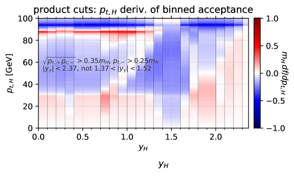
Figure 8: Upper plot: the $\cos\theta$ regions that are excluded by the main relevant photon $p_{t}$ and rapidity cuts, as a function of the Higgs boson rapidity $y_{\text{\sc h}}$, for $p_{t,\text{\sc h}}=0$. The vertical lines indicate the $y_{\text{\sc h}}$ values where pairs of cuts have equivalent actions, i.e. corresponding to the special cases outlined in sections 4.2 and 4.3. The lower plot shows the Born ($p_{t,\text{\sc h}}=0$) acceptance with these cuts, as a function of $y_{\text{\sc h}}$.

To help make this section’s discussion a bit more concrete, we conclude it with a worked example using a concrete set of cuts. We take the cuts used by the ATLAS collaboration Aaboud:2018xdt ; ATLAS:2019jst , $p_{t,+}>p_{t,\text{cut}}=0.35m_{\gamma\gamma}$, $p_{t,-}>0.25m_{\gamma\gamma}$, $|\eta_{\gamma}|\equiv|y_{\gamma}|<y_{\max}$ and excluding photons in the region $y_{1}<|\eta_{\gamma}|<y_{2}$, with $y_{1}=1.37$, $y_{2}=1.52$ and $y_{\max}=2.37$. The CMS collaboration uses a similar structure of cuts Sirunyan:2018kta , with the same value of $m_{\text{\sc h}}/4$ for the $p_{t,-}$ cut, $p_{t,\text{cut}}=m_{\gamma\gamma}/3$ and $y_{1}=1.4442$, $y_{2}=1.566$ and $y_{\max}=2.50$. Since we are considering just Higgs decays in this article, and not the background of continuum $\gamma\gamma$ production, we will work with the assumption $m_{\gamma\gamma}=m_{\text{\sc h}}$. The structures that we will identify at various different Higgs rapidities will remain the same for a general $m_{\gamma\gamma}$ as long as hardness cuts remain expressed as a fraction of $m_{\gamma\gamma}$.

Fig. 8 (upper plot) shows the regions of $\cos\theta$ that are excluded by the ATLAS cuts, as a function of the Higgs rapidity, for $p_{t,\text{\sc h}}=0$. The lower plot shows the resulting efficiency. Each value of $y_{\text{\sc h}}$ where two cuts intersect (so long as the intersection borders the allowed region) leads to one of the special configurations discussed in sections 4.2 and 4.3. Those $y_{\text{\sc h}}$ values are indicated with dashed vertical lines and they correspond to kinks in the $y_{\text{\sc h}}$-dependence of the acceptance. They arise at the midpoints between any pair of the (same-sign) rapidity cut values,

$$|y_{\text{\sc h}}|=\left\{\frac{y_{1}+y_{2}}{2}=1.445,\quad\frac{y_{1}+y_{\max}}{2}=1.87,\quad\frac{y_{2}+y_{\max}}{2}=1.945\right\},\quad$$ (62a)

and at each of the points where the rapidity cut and the main hardness cut are equivalent

$$|y_{\text{\sc h}}|=y_{\text{cut}}-\operatorname{arccosh}\frac{m_{\text{\sc h}}}{2p_{t,\text{cut}}}\simeq\left\{0.474,0.624,1.474\right\},$$ (62b)

where $y_{\text{cut}}$ is any of $y_{1}$, $y_{2}$ and $y_{\max}$.

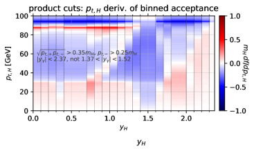
Figure 9: The $p_{t,\text{\sc h}}$ derivative of the acceptance, as a function of the Higgs boson rapidity (horizontal axis) and transverse momentum (vertical axis). Linear $p_{t,\text{\sc h}}$ dependence of the acceptance at small $p_{t,\text{\sc h}}$ appears as a blue or red colour that persists in the $p_{t,\text{\sc h}}\to 0$ limit. The upper plot shows the results for the standard ATLAS asymmetric cuts. The middle plot shows the results obtained replacing the $p_{t,+}>0.35m_{\text{\sc h}}$ cut with a product cut, $\sqrt{p_{t,-}p_{t,+}}>0.35m_{\text{\sc h}}$, while retaining the $p_{t,-}>0.25m_{\text{\sc h}}$ cut and all photon rapidity cuts. The lower plot shows the same results averaged over rapidity bins.

To help understand the $p_{t,\text{\sc h}}$ dependence of the cuts in different regions, Fig. 9 shows the $p_{t,\text{\sc h}}$ derivative of the acceptance,

$$m_{\text{\sc h}}\frac{df(p_{t,\text{\sc h}},y_{\text{\sc h}})}{dp_{t,\text{\sc h}}}\,,$$ (63)

as a function of $y_{\text{\sc h}}$ (horizontal axis) and $p_{t,\text{\sc h}}$ (vertical axis). The value of the derivative is encoded in the colour of the points. The top panel is for standard asymmetric cuts used by the ATLAS collaboration. The deep red colour at low $p_{t,\text{\sc h}}$, over a wide range of $y_{\text{\sc h}}$ values is the signal of linear dependence of the acceptance on the cuts. One also sees a complex structure of bands at higher $p_{t,\text{\sc h}}$ values, reflecting the interplay between the many rapidity and $p_{t}$ cuts.

The middle panel of Fig. 9 shows the result obtained if one replaces the asymmetric cuts with product cuts, $\sqrt{p_{t,-}p_{t,+}}>0.35m_{\text{\sc h}}$ and $p_{t,-}>0.25m_{\text{\sc h}}$, maintaining the ATLAS rapidity cuts. In the low $p_{t,\text{\sc h}}$ region, over most $y_{\text{\sc h}}$ values, one sees that the $p_{t,\text{\sc h}}$ derivative of the acceptance vanishes at $p_{t,\text{\sc h}}=0$, consistent with an overall quadratic $p_{t,\text{\sc h}}$ dependence of the acceptance. This pattern breaks down at each of the special rapidities highlighted with a vertical dashed line, i.e. the rapidities of Eq. (62), where one sees that the acceptance derivative remains non-zero all the way to $p_{t,\text{\sc h}}=0$, precisely as expected from our discussion in sections 4.2 and 4.3 (the $y_{\text{\sc h}}=1.445$ transition is too narrow to see with the plot’s resolution). The transition from quadratic to linear $p_{t,\text{\sc h}}$ dependence is at progressively higher $p_{t,\text{\sc h}}$ as one moves away from those $y_{\text{\sc h}}$ values. This is why, if we integrate over Higgs rapidity bins that are sufficiently large in those regions, e.g. $0.4{-}0.7$, $1.3{-}1.7$ and $1.7{-}2.1$, we expect to recover mild quadratic $p_{t,\text{\sc h}}$ dependence at low $p_{t,\text{\sc h}}$, with linear quadratic dependence setting in only for higher $p_{t,\text{\sc h}}$ values (e.g. $p_{t,\text{\sc h}}>\delta s_{0}/f_{0}m_{\text{\sc h}}$ in the case of the combination of hardness and rapidity cuts, for a rapidity bin of half-width $\delta$). This is illustrated in the bottom panel of Fig. 9 (the pattern of colours alone perhaps does not give full confidence that the linear term is consistent with zero, however an explicit inspection of the results in each rapidity bin confirms that this is indeed the case).

5 Compensating Boost Invariant cuts

We saw in section 3.5 that if one uses a hardness cut on the photon transverse momentum in the Collins-Soper frame, Eq. (39), the acceptance is independent of $p_{t,\text{\sc h}}$ at low $p_{t,\text{\sc h}}$. As it stands, that approach faces two problems. Firstly, at larger $p_{t,\text{\sc h}}$ values, the acceptance is noticeably lower than with other cuts. Secondly, as we saw in section 4.3, when combining a $p_{t,\text{\sc cs}}$ cut with rapidity cuts, the latter bring back $p_{t,\text{\sc h}}$ dependence of the acceptance at low $p_{t,\text{\sc h}}$. In this section, we will examine how to alleviate both of these problems, with techniques that balance loss and gain of acceptance from different decay phase space regions.

Achieving an acceptance that has no $p_{t,\text{\sc h}}$ dependence at low $p_{t,\text{\sc h}}$ has interesting implications. A first observation is that for experimental measurements that correct to a total cross section or an STXS cross section Berger:2019wnu , having an experimental acceptance that is independent of $p_{t,\text{\sc h}}$ removes one source of systematic (knowledge of the $p_{t,\text{\sc h}}$ distribution) in the extrapolation to the more inclusive cross section. The second observation concerns the perturbative structure of fiducial cross sections in the approximation that one can neglect the perturbative impact of isolation cuts. Consider an acceptance $f(p_{t,\text{\sc h}},y_{\text{\sc h}})$ that is independent of $p_{t,\text{\sc h}}$ and equal to $f_{0}(y_{\text{\sc h}})$ up to some threshold transverse momentum scale $p_{t}^{\text{thresh}}(y_{\text{\sc h}})$. Suppose that we know the Higgs cross section differentially in rapidity $d\sigma/dy_{\text{\sc h}}$ (integrated over $p_{t,\text{\sc h}}$) and differentially in both $p_{t,\text{\sc h}}$ and $y_{\text{\sc h}}$, $d\sigma/dp_{t,\text{\sc h}}dy_{\text{\sc h}}$. We can then write the fiducial cross section as

$$\sigma_{\text{fid}}=\int_{-\infty}^{\infty}dy_{\text{\sc h}}\frac{d\sigma}{dy_{\text{\sc h}}}f_{0}(y_{\text{\sc h}})-\int_{-\infty}^{\infty}dy_{\text{\sc h}}\int_{p_{t}^{\text{thresh}}(y_{\text{\sc h}})}^{\infty}\!\!\!\!\!\!\!\!dp_{t,\text{\sc h}}\frac{d\sigma}{dp_{t,\text{\sc h}}dy_{\text{\sc h}}}\left[f_{0}(y_{\text{\sc h}})-f_{0}(p_{t,\text{\sc h}},y_{\text{\sc h}})\right]\,,$$ (64)

where infinite integration limits are to be understood as extending to the kinematic limit. In this way of writing the fiducial cross section, there is no dependence at all on the details of the differential cross section at any $p_{t,\text{\sc h}}$ below $p_{t}^{\text{thresh}}(y_{\text{\sc h}})$.

Eq. (64) means that all problems of low-$p_{t,\text{\sc h}}$ acceptance-induced factorial divergences in the perturbative series disappear, and the only issues that remain in the fiducial cross section will be those intrinsic to hard cross sections. Based on the experience with rapidity differential Drell-Yan cross sections Dasgupta:1999zm , and assuming similar conclusions to be valid for Higgs production, one expects the first term in Eq. (64) to have renormalon power corrections of the form $(\Lambda/m_{\text{\sc h}})^{2}$ (within the caveats mentioned in Ref. Beneke:1998ui ). The work of Ref. FerrarioRavasio:2020guj ; Caola:2021kzt , on corrections to Drell-Yan production at finite $p_{t}$ was consistent with $(\Lambda/p_{t})^{2}$ corrections and if the conclusions apply also in the case of Higgs production, would imply power corrections to the second term that are no larger than $(\Lambda/p_{t}^{\text{thresh}})^{2}$. If $p_{t}^{\text{thresh}}$ is sufficiently large, the fiducial cross section should then have a perturbative description that is as reliable as that of a normal (rapidity-differential) total cross section.

A more general comment about Eq. (64) is that the dominant contribution will often come from the first term. The second term is suppressed for two reasons: firstly, for sufficiently large $p_{t}^{\text{thresh}}$, only a small fraction of the cross section is above $p_{t}^{\text{thresh}}$; secondly, in practice $f_{0}(p_{t,\text{\sc h}},y_{\text{\sc h}})$ is often numerically quite close to $f_{0}(y_{\text{\sc h}})$.

5.1 The case with just hardness cuts

As before when considering just hardness cuts, we work within a framework where the only experimental $p_{t}$ cut that is essential is that on $p_{t,-}$, i.e. there is some minimal $p_{t}$ below which the experiments cannot reliably reconstruct photons (or leptons, etc. as appropriate), but that apart from that we have complete flexibility with other cuts. We will start from the $p_{t,\text{\sc cs}}$ cut of section 3.5 and use the flexibility so as to enhance the size of the region at low and moderate $p_{t,\text{\sc h}}$ where the acceptance is exactly $p_{t,\text{\sc h}}$ independent, while at large values of $p_{t,\text{\sc h}}$ we will seek to make the acceptance as close as possible to that obtained with just a $p_{t,-}$ cut.

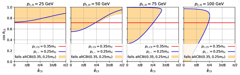
Figure 10: Action of the $p_{t,\text{\sc cs}}$ and $p_{t,-}$ cuts of section 3.5 in the $\bar{\phi}_{\text{\sc cs}}$–$\theta_{\text{\sc cs}}$ plane, as defined in Eq. (65), for four values of $p_{t,\text{\sc h}}$.

Given $\vec{p}_{t,\text{\sc cs}}$ from Eq. (39), it is helpful to define

$$\theta_{\text{\sc cs}}=\sin^{-1}\frac{2p_{t},\text{\sc cs}}{m_{12}}\,,\qquad\phi_{\text{\sc cs}}=\cos^{-1}\frac{\vec{\delta}_{t,12}\cdot\vec{p}_{t,12}}{\delta_{t,12}p_{t,12}}\,,\qquad\bar{\phi}_{\text{\sc cs}}=\min(\phi_{\text{\sc cs}},\pi-\phi_{\text{\sc cs}})\,,$$ (65)

such that $0<\theta_{\text{\sc cs}}<\pi/2$, $0<\phi_{\text{\sc cs}}<\pi$ and $0<\bar{\phi}_{\text{\sc cs}}<\pi/2$. Fig. 10 shows the $\bar{\phi}_{\text{\sc cs}}$–$\cos\theta_{\text{\sc cs}}$ plane for Higgs decay for several values of $p_{t,\text{\sc h}}$. Recall from the discussion of section 2 that the scalar nature of the Higgs boson results in uniform coverage of the plane. The figures shows the action of the cuts used in section 3.5, i.e. a $p_{t,\text{\sc cs}}\geq 0.35m_{\text{\sc h}}$ cut, which excludes the pink region, and a $p_{t,-}\geq 0.25m_{\text{\sc h}}$ cut, which excludes the blue region. The $p_{t,\text{\sc cs}}$ cut is, by construction, a horizontal line independent of $p_{t,\text{\sc h}}$. To understand the behaviour of the $p_{t,-}$ cut, it is useful to identify, as a function of $\phi_{\text{\sc cs}}$, the $\sin\theta_{\text{\sc cs}}$ values where $p_{t,-}=p_{t,-,\text{cut}}\equiv p_{t,\text{cut}}-\Delta$. There are two solutions for $\sin\theta_{\text{\sc cs}}$ and at low $p_{t,\text{\sc h}}$, only one of them is physical,

$$\sin\theta_{\text{\sc cs}}^{-}(\phi) =\frac{+2p_{t,\text{\sc h}}\sqrt{m_{\text{\sc h}}^{2}+p_{t,\text{\sc h}}^{2}}|\cos\phi|+\sqrt{U(\phi)}}{2m_{\text{\sc h}}^{2}+p_{t,\text{\sc h}}^{2}(1+\cos 2\phi)}\,,$$ (66a)

$$U(\phi) =2\left(p_{t,\text{\sc h}}^{2}\left(m_{\text{\sc h}}^{2}+4p_{t,-,\text{cut}}^{2}\right)\cos 2\phi-p_{t,\text{\sc h}}^{2}\left(m_{\text{\sc h}}^{2}-4p_{t,-,\text{cut}}^{2}\right)+8m_{\text{\sc h}}^{2}p_{t,-,\text{cut}}^{2}\right)\,,$$ (66b)

where for compactness, we have dropped the cs subscript on the $\phi$ and we write $p_{t,\text{\sc h}}$ and $m_{\text{\sc h}}$ rather than $p_{t,12}$ and $m_{12}$. For $p_{t,\text{\sc h}}=0$, $\sqrt{U}=4m_{\text{\sc h}}p_{t,-,\text{cut}}$ is the only contribution to the numerator, the physical solution is that with $+\sqrt{U}$ and we get $\sin\theta_{\text{\sc cs}}^{-}=2p_{t,-,\text{cut}}/m_{\text{\sc h}}$, as expected. Eq. (66) is the generalisation of the small-$p_{t,\text{\sc h}}$ expansion given in Eq. (6).

For $p_{t,\text{\sc h}}\geq p_{t,\text{\sc h}}^{\text{\sc cs}\text{-threshold}}\simeq 27\;\mathrm{GeV}$, cf. Eq. (40a), Fig. 10 illustrates how the $p_{t,-}$ cut starts to extend beyond the $p_{t,\text{\sc cs}}$ cut in the region around $\bar{\phi}_{\text{\sc cs}}=0$, which leads to the loss of efficiency that is visible in Fig. 6. Examining the low-$\bar{\phi}_{\text{\sc cs}}$ region in the $p_{t,\text{\sc h}}=50\;\mathrm{GeV}$ panel of Fig. 10, we notice that the phase space that has been lost for $\bar{\phi}_{\text{\sc cs}}<\pi/4$ can potentially be recovered by relaxing the $p_{t,\text{\sc cs}}$ cut for $\bar{\phi}_{\text{\sc cs}}>\pi/4$. Specifically if $\bar{\phi}_{\text{\sc cs}}>\pi/4$, we can determine the value of $\theta_{\text{\sc cs}}^{-}$ that would be obtained if one mirrored the $\phi$ value around $\pi/4$. Let us refer to that as

$$\theta_{\text{\sc cs}}^{m}=\theta_{\text{\sc cs}}^{-}(\pi/2-\bar{\phi}_{\text{\sc cs}})\,.$$ (67)

When $\cos\theta_{\text{\sc cs}}^{m}<f_{0}$, we can recover the phase space that was lost for $\bar{\phi}_{\text{\sc cs}}<\pi/4$ by allowing $\cos\theta_{\text{\sc cs}}$ values up to $2f_{0}-\cos\theta_{\text{\sc cs}}^{m}$ rather than the usual $f_{0}$. For typical cut values, the Born acceptance, $f_{0}$, is then retained as long as there is enough phase space at a given $\bar{\phi}_{\text{\sc cs}}>\pi/4$ to compensate for the phase space lost to the $p_{t,-}$ cut at the mirrored $\phi$ value. One requirement for this to be true is that $\cos\theta_{\text{\sc cs}}^{-}(\pi/4)>f_{0}$. For small values of $\Delta$, this is a sufficient requirement and the Born acceptance can be retained up to

$$p_{t,\text{\sc h}}=2\sqrt{2}\Delta+\sqrt{2}\frac{m_{\text{\sc h}}^{2}+4p_{t,\text{cut}}^{2}}{p_{t,\text{cut}}m_{\text{\sc h}}}\frac{\Delta^{2}}{m_{\text{\sc h}}}+\mathcal{O}_{3}\,,$$ (68)

rather than $2\Delta$ for the $p_{t,\text{\sc cs}}$ cut. (One can write the full expression for the transition point in closed form, but it is not especially illuminating). Fig. 10 is instructive also for thinking about how to maximise the acceptance for yet larger $p_{t,\text{\sc h}}$. In the $p_{t,\text{\sc h}}=75\;\mathrm{GeV}$ panel, one sees a region of $\bar{\phi}_{\text{\sc cs}}\gtrsim 5\pi/16$ where the $p_{t,-}$ cut is inactive, corresponding to negative values for $U(\bar{\phi}_{\text{\sc cs}})$ in Eq. (66). Such a region starts to appear for $p_{t,\text{\sc h}}>2p_{t,-,\text{cut}}$, as can be understood by substituting $\phi=\pi/2$ into Eq. (2) and observing that $p_{t,-}\geq p_{t,\text{\sc h}}/2$ for all $\theta$ values. This suggests a strategy whereby one ignores the $p_{t,\text{\sc cs}}$ cut altogether for $\phi_{\text{\sc cs}}$ values where $U(\phi_{\text{\sc cs}})$ is negative. Additionally, Fig. 10 shows that for large $p_{t,\text{\sc h}}$ values, the region excluded by the $p_{t,-}$ cut no longer extends to $\cos\theta_{CS}=1$. This occurs when the second solution for $\sin\theta_{\text{\sc cs}}$ that yields $p_{t,-}=p_{t,-,\text{cut}}$,

$$\sin\theta_{\text{\sc cs}}^{+}(\phi)=\frac{+2p_{t,\text{\sc h}}\sqrt{m_{\text{\sc h}}^{2}+p_{t,\text{\sc h}}^{2}}|\cos\phi|-\sqrt{U(\phi)}}{2m_{\text{\sc h}}^{2}+p_{t,\text{\sc h}}^{2}(1+\cos 2\phi)}\,,$$ (69)

is in the physical range $0<\sin\theta_{\text{\sc cs}}^{+}(\bar{\phi}_{\text{\sc cs}})<1$. This suggests a strategy whereby one accepts events with $\cos\theta_{\text{\sc cs}}>\cos\theta_{\text{\sc cs}}^{+}(\bar{\phi}_{\text{\sc cs}})$ whenever the latter is physical.

Algorithm 1 Hardness Compensating Boost-Invariant (CBI${}_{\text{H}}$) cut algorithm to determine whether an event with a two-body decay should be accepted. It takes a Born transverse-momentum threshold $p_{t\text{cut}}$ and a minimum $p_{t}$ requirement, $p_{t,-,\text{cut}}\equiv p_{t\text{cut}}-\Delta$ on both decay products.

1:  If $p_{t,-}<p_{t,-,\text{cut}}$ discard the event.

2:  If $p_{t,\text{\sc cs}}\geq p_{t,\text{cut}}$, with $p_{t,\text{\sc cs}}$ is defined in Eq. (39), accept the event.

3:  If either of $U(\bar{\phi}_{\text{\sc cs}})$ and $U(\pi/2-\bar{\phi}_{\text{\sc cs}})$ is negative, as obtained using Eqs. (65) and (66), accept the event.

4:  If $\sin\theta_{\text{\sc cs}}^{+}(\bar{\phi}_{\text{\sc cs}})$ in Eq. (69) is between $0$ and $1$ and $\cos\theta_{\text{\sc cs}}>\cos\theta_{\text{\sc cs}}^{+}(\bar{\phi}_{\text{\sc cs}})$, accept the event.

5:  If $\bar{\phi}_{\text{\sc cs}}>\pi/4$, determine the value of $\theta_{\text{\sc cs}}^{-}$, that would be obtained if one mirrored the $\phi$ value around $\pi/4$. We refer to it as $\theta_{\text{\sc cs}}^{m}=\theta_{\text{\sc cs}}^{-}(\pi/2-\bar{\phi}_{\text{\sc cs}})$. If $\cos\theta_{\text{\sc cs}}^{m}<f_{0}$, accept the event if $\cos\theta_{\text{\sc cs}}<2f_{0}-\cos\theta_{\text{\sc cs}}^{m}$.

6:  Reject the event.

Assembling together these different elements, we obtain a hardness compensating boost-invariant (CBI${}_{\text{H}}$) cut procedure for selecting $H\to\gamma\gamma$ events, given as Algorithm 1.

Figure 11: Action of the hardness-compensating boost-invariant (CBI${}_{\text{H}}$) cuts in the $\bar{\phi}_{\text{\sc cs}}$–$\theta_{\text{\sc cs}}$ plane, as compared to the $p_{t,\text{\sc cs}}$ and $p_{t,-}$ cuts of section 3.5, whose action was shown in Fig. 10.

It is generally speaking sensible to apply this algorithm if $2\sqrt{2}(p_{t,\text{cut}}-p_{t,-,\text{cut}})\equiv 2\sqrt{2}\Delta\lesssim 2p_{t,-,\text{cut}}$. The action of the CBI${}_{\text{H}}$ cut procedure on the decay phase space is shown in Fig. 11. In the $p_{t,\text{\sc h}}=25\;\mathrm{GeV}$ panel, one sees that the $p_{t,\text{\sc cs}}$ cut (red line) controls the acceptance. In the $p_{t,\text{\sc h}}=50\;\mathrm{GeV}$ panel, the right hand part of the plot illustrates the use of the region of $\phi>\pi/4$ between the red line and the orange band (a region that is accepted) that compensates for the loss of the region below the red line due to the $p_{t,-}$ cut. In the remaining two panels, one sees how the CBI${}_{\text{H}}$ cut almost fully tracks the $p_{t,-}$ cut, allowing for maximisation of the acceptance.

Figure 12: Acceptance of the hardness compensating boost-invariant (CBI${}_{\text{H}}$) cut, as a function of $p_{t,\text{\sc h}}$, compared to the product cuts of section 3.2 and the maximum possible acceptance that can be achieved with the underlying $p_{t,-}>0.25m_{\text{\sc h}}$ requirement.

The resulting acceptance as a function of $p_{t,\text{\sc h}}$ is shown in Fig. 12 for our usual pair of cut thresholds. The acceptance is exactly independent of $p_{t,\text{\sc h}}$ up to $p_{t,\text{\sc h}}\simeq 60\;\mathrm{GeV}$ (which, numerically, is substantially larger than the naive expectation of $2\sqrt{2}{\Delta}\simeq 35\;\mathrm{GeV}$). This exact independence ensures that the perturbative series for the fiducial cross section should be independent of the acceptance-induced alternating-sign factorial divergence discussed in sections 2 and 3. At higher $p_{t,\text{\sc h}}$ values, the acceptance then closely tracks the maximum possible acceptance that can be obtained with the $p_{t,-}$ cut. Thus the CBI${}_{\text{H}}$ cut is near optimal.

For all of the other hardness cuts considered so far, we have included equations such as Eq. (2.3) and plots such as Fig. 3 to illustrate the perturbative behaviour of the cuts. For CBI${}_{\text{H}}$ cuts with the standard thresholds, the terms in the perturbative series are essentially zero and the N3LL and N3LO acceptance corrections are zero for $\epsilon\lesssim m_{\text{\sc h}}/2$: the fact that $f(p_{t,\text{\sc h}})=f_{0}$ for $p_{t,\text{\sc h}}\lesssim m_{\text{\sc h}}/2$ ensures that the integrand of Eq. (23) is zero. Were we to extend the integral to the kinematic limit in $p_{t,\text{\sc h}}$, using a matched fixed-order plus resummation $p_{t,\text{\sc h}}$ distribution, the coefficients of the perturbative expansion would be non zero, but they would show the convergence properties of a high-$p_{t,\text{\sc h}}$ cross section, as expected from Eq. (64).

5.2 The case with hardness and rapidity cuts

In section 5.1 we worked with the assumption that there is a non-negotiable minimum $p_{t}$ cut on the softer decay product and adjusted the $p_{t,\text{\sc cs}}$ cut to retain a boost-invariant acceptance over a wide range of $p_{t,\text{\sc h}}$ values. Here we extend this approach, working with the additional constraint that there are non-negotiable rapidity cuts on the decay products, but still using adjustments of the $p_{t,\text{\sc cs}}$ cut (or, more directly, of the $\cos\theta_{\text{\sc cs}}$ cut) to attempt to retain a $p_{t,\text{\sc h}}$-independent acceptance.

The starting point is to establish the $\theta_{\text{\sc cs}}$ values for which a decay product can be at the boundary of a cut $y_{\text{cut}}$. For any given decay $\phi$ there are up to two solutions,

$$\sin\theta_{\text{\sc cs}}^{y_{\text{cut}}}(\phi)=\frac{2s\,p_{t,\text{\sc h}}\sqrt{m_{\text{\sc h}}^{2}+p_{t,\text{\sc h}}^{2}}\cos\phi\pm\sqrt{V(\phi)}}{p_{t,\text{\sc h}}^{2}+p_{t,\text{\sc h}}^{2}\cos 2\phi+2m_{\text{\sc h}}^{2}(1+c^{2})\,,}\,,\qquad s=\left\{\begin{array}[]{c}+1\text{ for $y_{\text{\sc h}}<y_{\text{cut}}$}\,,\\[5.0pt] -1\text{ for $y_{\text{\sc h}}>y_{\text{cut}}$}\,,\end{array}\right.$$ (70a)

where

$$V(\phi)=2m_{\text{\sc h}}^{2}(1+c^{2})\left[p_{t,\text{\sc h}}^{2}(\cos 2\phi-1)+2m_{\text{\sc h}}^{2}c^{2}\right]\,,\,\qquad c=\frac{1}{\sinh(y_{\text{cut}}-y_{\text{\sc h}})}\,.$$ (70b)

A solution that gives $\sin\theta_{\text{\sc cs}}^{y_{\text{cut}}}(\phi)>1$ ($<0$) is considered to be at $\sin\theta_{\text{\sc cs}}=1$ ($0$). Taking the case $y_{\text{\sc h}}<y_{\text{cut}}$, a requirement $y_{\gamma}<y_{\text{cut}}$ implies a veto on $\theta_{\text{\sc cs}}$ values that lie between the two solutions. If $V(\phi)$ is negative, all $\theta_{\text{\sc cs}}$ values are allowed.

One immediate difference relative to the case of just hardness cuts (Eqs. (66, 69)) is that Eq. (70) contains dependence on $\cos\phi$ rather than $|\!\cos\phi|$, with the result that configurations at $\phi$ and $\pi-\phi$ are not equivalent. Consequently, it will be useful for our compensation algorithm to consider four points in $\phi$ simultaneously rather than just two. For any given $\phi$, the four points will be

$$\phi_{\{1,2,3,4\}}=\{\phi,\,\pi-\phi,\,|\pi/2-\phi|,\,\pi-|\pi/2-\phi|\}\,,$$ (71)

recalling that from Eq. (65) we have $0<\phi<\pi$. Eq. (71) ensures that we consider points with opposite signs but equal values of both $\cos\phi$ and $\cos 2\phi$.

Another difference relative to the case of just hardness cuts is the extra degree of complexity brought in by the presence of multiple rapidity cuts and the interplay between different rapidity cuts and the hardness cuts (cf. Fig. 8, even just for $p_{t,\text{\sc h}}=0$). This leads us to formulate a balancing procedure where the adjustments can largely be automated.

For this purpose, we use $\mathcal{R}_{i}(\phi,p_{t,\text{\sc h}})$ to denote the region(s) of $\cos\theta_{\text{\sc cs}}$ values allowed by cut $i$ for a given $\phi$ and $p_{t,\text{\sc h}}$ (for example, an allowed region might consist of a segment from $\cos\theta_{\text{\sc cs}}=0$ to $0.5$ and another segment from $0.8$ to $1.0$). We also introduce the notation $\mathcal{E}(\mathcal{R})$ to denote the total extent of allowed region $\mathcal{R}$ ($\mathcal{E}(\mathcal{R})=0.7$ in the example just given). For a scalar decay, that extent is equal to the average acceptance given the boson kinematic variables and the decay $\phi$. Finally, regions can be combined logically, for example for cuts $a$ and $b$, we write $\mathcal{R}_{a,b}(\phi,p_{t,\text{\sc h}})$ to indicate the region(s) in $\cos\theta_{\text{\sc cs}}$ where a decay passes both sets of cuts. In practice when combining multiple cuts, the final allowed region may contain multiple non-contiguous allowed segments in $\cos\theta_{\text{\sc cs}}=0$, which would be analytically tedious to deal with, but can easily be encapsulated in computer code. We will use $\mathcal{R}_{-,\forall y}(\phi,p_{t,\text{\sc h}})$ to denote the region that is allowed after applying the $p_{t,-}$ cut and all photon rapidity cuts, and $\mathcal{R}_{\text{\sc cs},-,\forall y}(\phi,p_{t,\text{\sc h}})$ to denote the region that remains when additionally applying the $p_{t,\text{\sc cs}}$ cut. As part of our high-$p_{t}$ enhancement approach, for the purpose of the compensation calculations, $\mathcal{R}_{-}(\phi)$ will be evaluated with the replacement $\cos\theta_{\text{\sc cs}}^{+}(\phi)\to 1$. With the notation established, we can present our hardness and rapidity compensating boost-invariant algorithm (CBI${}_{\text{HR}}$), algorithm 2 on p. 2.

Algorithm 2 Hardness and Rapidity Compensating boost-invariant (CBI${}_{\text{HR}}$) cut algorithm. It takes a primary transverse-momentum threshold $p_{t,\text{cut}}$, applied by default to $p_{t,\text{\sc cs}}$, a minimum $p_{t}$ requirement, $p_{t,-,\text{cut}}\equiv p_{t\text{cut}}-\Delta$ on both decay products, and a set of rapidity cuts.

1:  If $p_{t,-}<p_{t,-,\text{cut}}$ or either of the decay products fails the rapidity cuts, discard the event.

2:  Use Eq. (65) to determine the Collins-Soper decay angles (we refer to $\phi_{\text{\sc cs}}$ as just $\phi$).

3:  Apply high-$p_{t}$ enhancement: using Eq. (66), if $U(\phi_{i})<0$ for any of the $\phi_{i}$ in Eq. (71), accept the event; using Eq. (69), if $\cos\theta_{\text{\sc cs}}>\cos\theta_{\text{\sc cs}}^{+}(\phi_{1})$, accept the event.

4:  Evaluate what the $p_{t,\text{\sc h}}=0$ acceptance extent would be for this $\phi$, $f_{0}=\mathcal{E}(\mathcal{R}_{\text{\sc cs},-,\forall y}(\phi,p_{t,\text{\sc h}}=0))$.

5:  For each of the original and mirrored $\phi_{i}$ values in Eq. (71), evaluate the acceptance extents both with and without the $p_{t,\text{\sc cs}}$ cut

$$f_{i,\text{\sc cs}}=\mathcal{E}(\mathcal{R}_{\text{\sc cs},-,\forall y}(\phi_{i},p_{t,\text{\sc h}}))\,,\qquad f_{i}=\mathcal{E}(\mathcal{R}_{-,\forall y}(\phi_{i},p_{t,\text{\sc h}}))\,.$$ (72)

6:  Determine the sums of the acceptance extents $f_{\Sigma,\text{\sc cs}}=\sum_{i=1}^{4}f_{i,\text{\sc cs}}$ and $f_{\Sigma}=\sum_{i=1}^{4}f_{i}$.

7:  If $f_{\Sigma,\text{\sc cs}}>4f_{0}$, additional vetoes are needed, which should total $f_{v}=f_{\Sigma,\text{\sc cs}}-4f_{0}$ when summed across the four $\phi_{i}$ values. The extent of the additional veto to be applied to this $\phi$ value is,

$$\delta f_{1}^{(v)}=f_{v}\frac{\max(0,f_{1,\text{\sc cs}}-f_{0})}{\sum_{i=1}^{4}\max(0,f_{i,\text{\sc cs}}-f_{0})}\,.$$ (73)

We choose to apply it from the uppermost part of the allowed $\mathcal{R}_{\text{\sc cs},-,\forall y}(\phi_{1},p_{t,\text{\sc h}})$ region, working downwards. Accept the event iff $\theta_{\text{\sc cs}}$ is in the allowed region $\mathcal{R}_{\text{\sc cs},-,\forall y}(\phi_{1},p_{t,\text{\sc h}})$ but not in the additionally vetoed region.

8:  If $f_{\Sigma,\text{\sc cs}}<4f_{0}$, one should attempt to find additional acceptance. The total additional acceptance needed across all four $\phi_{i}$ values is $f_{a}=4f_{0}-f_{\Sigma,\text{\sc cs}}$. The maximum recoverable acceptance, through elimination of the $p_{t,\text{\sc cs}}$ cut, is $f_{\Sigma}-f_{\Sigma,\text{\sc cs}}$. If $f_{a}$ is larger than this maximum recoverable acceptance, discard the $p_{t,\text{\sc cs}}$ cut, and accept the event iff $\theta_{\text{\sc cs}}$ is in the $\mathcal{R}_{-,\forall y}(\phi_{1},p_{t,\text{\sc h}})$ region. Otherwise recover an additional acceptance

$$\delta f_{1}^{(a)}=f_{a}\frac{f_{1}-f_{1,\text{\sc cs}}}{\sum_{i=1}^{4}(f_{i}-f_{i,\text{\sc cs}})}\,,$$ (74)

for this $\phi$ value. We choose to do so working upwards from the lowermost $\cos\theta_{\text{\sc cs}}$ part of the difference between the $\mathcal{R}_{-,\forall y}(\phi_{1},p_{t,\text{\sc h}})$ and $\mathcal{R}_{\text{\sc cs},-,\forall y}(\phi_{1},p_{t,\text{\sc h}})$ regions. Accept the event iff $\theta_{\text{\sc cs}}$ is in $\mathcal{R}_{\text{\sc cs},-,\forall y}(\phi_{1},p_{t,\text{\sc h}})$ or the additional allowed region.

While the algorithm may appear to quite lengthy at first sight, its two underlying principles are simple: (1) within each group of mirror $\phi$ values, adjust the $\theta_{\text{\sc cs}}$ cuts so as to retain the same acceptance summed across those $\phi$ values as is obtained at $p_{t,\text{\sc h}}=0$; and (2) for $p_{t,\text{\sc h}}$ values above $2p_{t,-,\text{cut}}$, which is when $U(\phi)$ in Eq. (66b) can start to be negative, start relaxing the $\theta_{\text{\sc cs}}$ cut so as to bring the acceptance close to its maximal value without any $\theta_{\text{\sc cs}}$ cut.

There is one context where Algorithm 2 cannot maintain constant acceptance away from $p_{t,\text{\sc h}}=0$, specifically when the acceptance is limited by a pair of rapidity cuts, $y_{\gamma}>y_{\text{\sc h}}-Y$ and $y_{\gamma}<y_{\text{\sc h}}+Y$ for some $Y>0$. Considering, as before, the ATLAS $H\to\gamma\gamma$ cuts, cf. Fig. 8, this occurs for $|y_{H}|=1.945$, i.e. midway between the $|y_{\gamma}|>1.52$ and $|y_{\gamma}|<2.37$ cuts. In such a situation, examining just the term linear in $p_{t,\text{\sc h}}$ in Eq. (70a), one can see that for $\cos\phi>0$ the $y_{\gamma}<y_{\text{\sc h}}+Y$ condition raises the effective $\sin\theta_{\text{\sc cs}}$ cut, while for $\cos\phi<0$ the $y_{\gamma}>y_{\text{\sc h}}-Y$ cut raises the effective $\sin\theta_{\text{\sc cs}}$ cut. This means that taking $p_{t,\text{\sc h}}$ slightly away from zero always raises the effective $\sin\theta_{\text{\sc cs}}$ cut and so reduces the acceptance. With the default $p_{t,\text{\sc cs}}$ cut imposing a less stringent condition on $\theta_{\text{\sc cs}}$ in this region than the rapidity cuts, adjusting the $p_{t,\text{\sc cs}}$ cut as a function of $p_{t,\text{\sc h}}$ cannot recover the acceptance that is being lost.

A workaround for this issue is to raise the Born $p_{t,\text{\sc cs}}$ cut in a suitable rapidity region. One might worry about the resulting loss of acceptance, but as we shall see, this is minimal. For a generic situation with an overall rapidity cut $|y_{\gamma}|<y_{\max}$ and an exclusion band $y_{1}<|y_{\gamma}|<y_{2}$ ($y_{1,2,\max}=1.37,1.52,,2.37$ for ATLAS), we adopt the following procedure: starting from the midpoint between $y_{1}$ and $y_{\max}$ (where it is the $y_{2}$ cut that sets the Born acceptance) we replace the usual Born $p_{t,\text{\sc cs}}$ cut with the requirement (still supplemented with $p_{t,\text{\sc h}}$-dependent compensation)

$$p_{t,\text{\sc cs}}>\frac{m_{\text{\sc h}}}{2\cosh(y_{m}-y_{2})}\simeq 0.471m_{H}\,,\qquad\text{for }|y_{\text{\sc h}}|>y_{m}=\frac{y_{1}+y_{\max}}{2}\,.$$ (75)

This corresponds to a constraint on $\cos\theta$ that is identical to that of the $y_{2}$ cut at $y_{H}=y_{m}$. The impact of this modification is illustrated for $p_{t,\text{\sc h}}=0$ in the upper panel of Fig. 13 and it corresponds to the difference between the red and blue lines for $y_{\text{\sc h}}\simeq 1.9$, confirming that it is a small overall effect.

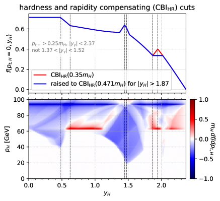
Figure 13: Analogue of Figs. 8 and 9, for the hardness and rapidity compensating boost-invariant (CBI${}_{\text{HR}}$) cuts. The upper panel shows the impact on the $p_{t,\text{\sc h}}=0$ acceptance of the raised high-rapidity $p_{t,\text{\sc cs}}$ cut that we impose, Eq. (75). The lower panel shows the $p_{t,\text{\sc h}}$ derivative of the acceptance (including the raised high-rapidity $p_{t,\text{\sc cs}}$ cut), illustrating that up to $p_{t,\text{\sc h}}\simeq 20\;\mathrm{GeV}$ the acceptance is independent of $p_{t,\text{\sc h}}$ for all Higgs rapidities. Absolute values of the acceptances as a function of $p_{t,\text{\sc h}}$ are to be found in Fig. 14.

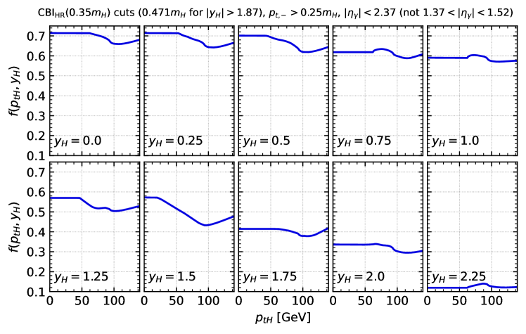
Figure 14: Acceptance for the hardness and rapidity compensating cuts, as a function of $p_{t,\text{\sc h}}$, for several $y_{\text{\sc h}}$ values (CBI${}_{\text{HR}}$, raised at high rapidity, as for the blue curve and the heat-map plot in the upper and lower panels respectively of Fig. 13).

The lower panel of Fig. 13 shows the $p_{t,\text{\sc h}}$ derivative of the acceptance, while the absolute values of the acceptances as a function of $p_{t,\text{\sc h}}$ are shown for a representative set of $y_{\text{\sc h}}$ values in Fig. 14. One of the key objectives of this section was to eliminate all $p_{t,\text{\sc h}}$ dependence at low-$p_{t,\text{\sc h}}$. Regions with no $p_{t,\text{\sc h}}$ dependence appear in white in Fig. 13, and the figure clearly demonstrates that the acceptance in the low and moderate $p_{t,\text{\sc h}}$ regions is independent of $p_{t,\text{\sc h}}$. The lowest value of $p_{t,\text{\sc h}}$ where this independence breaks down, corresponding to the $p_{t}^{\text{thresh}}$ threshold that enters into our expression, Eq. (64), for the fiducial cross section, is about $20\;\mathrm{GeV}$. It arises at the $y_{\text{\sc h}}$ value where the $p_{t,\text{\sc cs}}$ and the upper rapidity cuts have equivalent $p_{t,\text{\sc h}}=0$ actions, i.e. for $y_{H}=y_{\max}-\operatorname{arccosh}(m_{\text{\sc h}}/2p_{t,\text{cut}})\simeq 1.474$. For low values of $p_{t,\text{\sc h}}$, the compensation mechanism balances a loss of acceptance from the rapidity cut at $\phi>\pi/2$ (cf. the linear term of Eq. (42)), with a corresponding gain of acceptance from a loosening of the $p_{t,\text{\sc cs}}$ cut for $\phi<\pi/2$. However that compensation mechanism becomes compromised for

$$p_{t,\text{\sc h}}\gtrsim\frac{2\Delta}{1+f_{0}^{2}}+\mathcal{O}_{2}\,,$$ (76)

where, for $\phi=0$, the $\cos\theta$ limit from the $p_{t,-}$ cut, Eq. (16b), becomes lower than the $\cos\theta$ limit that is needed to balance the loss of acceptance from the rapidity cut for $\phi=\pi$.

6 Comments on Drell–Yan ($Z$) production

A complete study of the Drell–Yan process, i.e. the production of a charged-lepton pair, is beyond the scope of this article. Still it may be useful to briefly outline some of the similarities and differences relative to the Higgs production case. A first consideration is that the Drell-Yan di-lepton mass ($m_{{\ell\ell}}$) spectrum covers a continuum. We will work within the assumption that one picks a narrow part of the continuum (e.g. concentrating on resonant $Z$ production and/or imposing a narrow $m_{\ell\ell}$ window), or that hardness cuts are formulated as fractions of $m_{\ell\ell}$. This serves to avoid the additional complications that come from the interplay between a steeply-falling spectrum and fixed lepton hardness cuts. We will also ignore contributions from $\gamma\gamma\to\ell^{+}\ell^{-}$ (see e.g. Ref. Harland-Lang:2020veo ) and other electroweak contributions Denner:2011vu ; Frederix:2020nyw . This allows us to adopt the widespread parametrisation of the cross section as a function of the Drell–Yan exchanged 4-momentum $q$ and the Collins-Soper Collins:1977iv angles $\theta$ and $\phi$

$$\frac{d\sigma}{d^{4}qd\cos\theta d\phi}=\frac{3}{16\pi}\frac{d\sigma^{\text{unpol.}}}{d^{4}q}\left(h_{u}(\theta,\phi)+\sum_{i=0}^{7}A_{i}(q)\,h_{i}(\theta,\phi)\right),$$ (77)

in terms of the unpolarised cross section and the spherical harmonic functions $h_{\text{\sc x}}$

$$h_{u} =1+\cos^{2}\theta\,, h_{0} ={\textstyle\frac{1}{2}}(1-3\cos^{2}\theta)\,, h_{1} =\sin 2\theta\cos\phi\,,$$ (78a)

$$h_{2} ={\textstyle\frac{1}{2}}\sin^{2}\theta\cos 2\phi\,, h_{3} =\sin\theta\cos\phi\,, h_{4} =\cos\theta,$$ (78b)

$$h_{5} =\sin^{2}\theta\sin 2\phi\,, h_{6} =\sin 2\theta\sin\phi\,, h_{7} =\sin\theta\sin\phi\,.$$ (78c)

Each of the $h_{i}$ is multiplied by a coefficient $A_{i}(q)$, where we have made explicit that it depends on the Drell-Yan pair 4-momentum, while the normalisation of $h_{u}$ is fixed by the requirement for the expression to integrate to the unpolarised cross section. The $A_{i}(q)$ coefficients have been calculated to NNLO for non-zero $q_{t}$ in Ref. Gauld:2017tww . We will work within the assumption that the Drell-Yan lepton-pair transverse momentum, $p_{t,{\ell\ell}}$, is identical to $q_{t}$, which corresponds to an assumption that collinear photon radiation has been clustered with the leptons (we ignore lepton isolation). The Drell–Yan fiducial cross section with cuts on the final-state leptons is then given by

$$\frac{d\sigma_{\text{fid}}}{d^{4}q}=\frac{d\sigma^{\text{unpol.}}}{d^{4}q}\left[f^{(u)}(q)+\sum_{i=0\ldots 7}A_{i}(q)f^{(i)}(q)\right],$$ (79)

with

$$f^{(\text{{x}})}(q)=\frac{3}{16\pi}\int_{-1}^{1}\!d\!\cos\theta\int_{-\pi}^{\pi}\!d\phi\,\,h_{\text{{x}}}(\theta,\phi)\,\,\Theta_{\text{cuts}}(\theta,\phi,q)\,,$$ (80)

where $\Theta_{\text{cuts}}(\theta,\phi,q)$ is $1$ ($0$) if the leptons pass (do not pass) the fiducial cuts. We refer to the $f^{(\text{{x}})}$ as harmonic acceptances.

To understand the overall behaviour of the cross section, one needs to put together the behaviour of both the $A_{i}(q)$ and the $f^{(\text{{x}})}$ functions, and there are some general features that are worth keeping in mind. Firstly, for $i=3,\ldots,7$, the $f^{(i)}$ are zero, which can be seen by observing that the cuts have an effect that is unchanged under symmetry operations that swap the two leptons ($\theta\to\pi-\theta$ and $\phi\to\pi+\phi$) or that correspond to a change of the sign of $\phi$. Under one or other of these symmetry operations the corresponding $h_{i}$ functions flip sign. Secondly, the discussions of Refs. Collins:1978yt ; Boer:2006eq ; Berger:2007si ; Bodek:2010qg ; Lindfors:1979rc indicate that the $A_{0\ldots 2}$ are zero for $p_{t,\ell\ell}=0$ and that for small $p_{t,\ell\ell}$, the $A_{0}$ and $A_{2}$ coefficients scale quadratically with $p_{t,\ell\ell}$, while $A_{1}$ scales linearly.

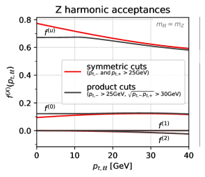
Figure 15: Left: acceptances for the non-zero spherical harmonics, as defined in Eq. (80), for symmetric cuts ($p_{t,\ell}>25\;\mathrm{GeV}$, in red), and product cuts ($\sqrt{p_{t,+}p_{t,-}}>30\;\mathrm{GeV}$, supplemented with a minimum cut $p_{t,-}>25\;\mathrm{GeV}$, in black). Right: the unpolarised part of the cross section (i.e. corresponding to $f^{(u)}$) within an all-order N3LL calculation (in blue) and its truncation at N3LO (in red), as a function of the minimum $p_{t,\ell\ell}$ that is allowed in the integration. The results are shown for the same symmetric and product cuts as in the left-hand plot.

As in our discussion of Higgs boson cuts, we start by considering just hardness cuts, using symmetric and product cuts for our illustration. Fig. 15 (left) shows the harmonic acceptances for symmetric cuts ($p_{t,\ell}>25\;\mathrm{GeV}$, as used by CMS Sirunyan:2019bzr ) and product cuts ($\sqrt{p_{t,+}p_{t,-}}>30\;\mathrm{GeV}$ and $p_{t,-}>25\;\mathrm{GeV}$). One clearly sees a linear $p_{t,\ell\ell}$ dependence for $f^{(u)}$ and $f^{(0)}$ for the symmetric cuts, which appears for the same reasons as discussed in the Higgs boson case (though with different coefficients). With product cuts, the linear dependence is absent for $p_{t,\ell\ell}\lesssim 2\Delta=10\;\mathrm{GeV}$, and it is only quadratic dependence that remains there.

The impact of the cuts on a perturbative calculation of the fiducial cross section is illustrated with the following series for the symmetric cuts (the spectrum and expansion used to obtain the N3LL results were kindly provided by the authors of Ref. Bizon:2018foh )

$$\frac{\sigma_{\text{sym}}^{\text{(u)}}-f_{0}\sigma_{\text{inc}}}{\sigma_{0}f_{0}} \simeq-0.074_{\alpha_{s}}+0.051_{\alpha_{s}^{2}}-0.057_{\alpha_{s}^{3}}+0.090_{\alpha_{s}^{4}}-0.181_{\alpha_{s}^{5}}+\ldots \simeq-0.047\;\; @\text{DL},$$

$$\simeq-0.074_{\alpha_{s}}+0.027_{\alpha_{s}^{2}}-0.014_{\alpha_{s}^{3}}+0.010_{\alpha_{s}^{4}}-0.010_{\alpha_{s}^{5}}+\ldots \simeq-0.055\;\; @\text{LL},$$

$$\simeq-0.118_{\alpha_{s}}+0.012_{\alpha_{s}^{2}}-0.016_{\alpha_{s}^{3}}+\ldots \simeq-0.114\;\; @\text{NNLL},$$

$$\simeq-0.118_{\alpha_{s}}+0.012_{\alpha_{s}^{2}}-0.016_{\alpha_{s}^{3}}+\ldots \simeq-0.114\;\; @\text{N3LL}.$$

It is the linear dependence of $f^{(u)}$ that will be critical, so the above equations show just the contribution to the cross section from $f^{(u)}$. The DL and LL results both show a breakdown in the convergence of the series, though at somewhat different orders and with fairly different normalisations for the smallest term. Considering the N3LL series, the all-order N3LL result and its N3LO truncation disagree at the order of a percent relative to the Born cross section.

The dependence of the unpolarised part of the fiducial cross section on a $p_{t,{\ell\ell}}$ cutoff and the impact of scale variation are illustrated in Fig. 15 (right). The N3LO truncation is noticeably sensitive to the minimum $p_{t,\ell\ell}$ allowed in the integration, converging only when including unphysically low values down to $1\;\mathrm{MeV}$ and below. The pattern can be compared to that in Fig. 3 (Higgs production with asymmetric cuts). The normalisation of the discrepancy here is much reduced because of the $C_{F}$ factor instead of a $C_{A}$ factor in the resummation (keeping in mind that the missing DL terms, i.e. those from N4LO onwards, scale as the colour factor to the fourth power). However, the accuracy of the data is also much higher for $Z$ production than for Higgs production, and so percent-level issues are conceivably relevant for the $Z$ case. The minimum $p_{t,\ell\ell}$ value that is needed for a reliable estimate of the N3LO coefficient is similar to that in the Higgs case, Eq. (21), because it is determined by the number of logarithms in the fixed-order expansion, which is the same.

The corresponding results for product cuts are

$$\frac{\sigma_{\text{prod}}^{\text{(u)}}-f_{0}\sigma_{\text{inc}}}{\sigma_{0}f_{0}} \simeq-0.006_{\alpha_{s}}-0.000_{\alpha_{s}^{2}}+0.000_{\alpha_{s}^{3}}-0.000_{\alpha_{s}^{4}}-0.000_{\alpha_{s}^{5}}+\ldots \simeq-0.006\;\; @\text{DL},$$

$$\simeq-0.006_{\alpha_{s}}-0.000_{\alpha_{s}^{2}}-0.000_{\alpha_{s}^{3}}+0.000_{\alpha_{s}^{4}}-0.000_{\alpha_{s}^{5}}+\ldots \simeq-0.007\;\; @\text{LL},$$

$$\simeq-0.018_{\alpha_{s}}-0.009_{\alpha_{s}^{2}}-0.003_{\alpha_{s}^{3}}+\ldots \simeq-0.030\;\; @\text{NNLL},$$

$$\simeq-0.018_{\alpha_{s}}-0.009_{\alpha_{s}^{2}}-0.002_{\alpha_{s}^{3}}+\ldots \simeq-0.029\;\; @\text{N3LL}.$$

The DL and LL results converge fast, while the N3LL resummation and its N3LO truncation agree at the per-mil level. From Fig. 15 (right), we see that the fiducial cross section (whether at all orders or N3LO) is essentially insensitive to transverse momenta below $10\;\mathrm{GeV}$.

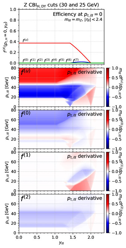
Figure 16: Top panels: $p_{t,\ell\ell}=0$ harmonic acceptances for $Z\to\ell^{+}\ell^{-}$, as defined in Eq. (80), for each of the spherical harmonic functions in Eq. (78). Lower panels: the $p_{t,\ell\ell}=0$ derivatives of the acceptances for the $f^{(\textsc{x})}$ that are non-zero. The left-hand column shows results for product cuts, the right-hand column for the CBI${}_{\text{H}}$ cuts supplemented with the condition in Eq. (83) (which, together, we refer to as CBI${}_{\text{H,DY}}$ cuts). In both figures we use events with a fixed $m_{{\ell\ell}}=m_{Z}=91.1876\;\mathrm{GeV}$.

If product cuts are to be a good replacement for standard symmetric and asymmetric cuts in $Z$-production studies, then one should understand their interplay with lepton rapidity cuts. Fig. 16 (left) examines the behaviour of the product cuts when supplemented with a requirement $|y_{\ell}|<y_{\max}=2.4$, as used by CMS Sirunyan:2019bzr . The top panel shows the harmonic acceptances for $p_{t,\ell\ell}=0$, as a function of the lepton-pair rapidity. The remaining panels show the $p_{t,\ell\ell}$ derivative of the acceptance for those harmonics that are non-zero. We comment on two features: firstly, $f^{(u)}$ acquires linear dependence at $y_{\ell\ell}=y_{t}\equiv y_{\max}-\operatorname{arccosh}(m_{\ell\ell}/2p_{t,\text{cut}})\simeq 1.42$. As with the analogous characteristic seen in sections 4.3 and 4.4, a suitably wide rapidity bin around this point will transform this linear dependence into reasonably tame quadratic dependence. The second feature concerns $f^{(1)}$, where one sees linear $p_{t,{\ell\ell}}$ dependence for $y_{\ell\ell}\geq y_{t}$. Recalling from our discussion above that $f^{(1)}(p_{t,{\ell\ell}})$ multiplies $A_{1}(p_{t,{\ell\ell}})$ and that the latter goes at most as $p_{t,{\ell\ell}}$ for small $p_{t,{\ell\ell}}$, the net effect on the cross section will remain quadratic. Thus we conclude that combining product hardness cuts with standard lepton rapidity cuts, one obtains quadratic dependence of the full acceptance on $p_{t,{\ell\ell}}$, as long as one uses suitably wide rapidity binning for the lepton pair around $y_{t}$. This should ensure that the good perturbative behaviour of product cuts illustrated in Fig. 15 (right) carries over to the case also with rapidity cuts.

The last question that we touch on concerns the design of cuts for which the acceptance is independent of $p_{t,{\ell\ell}}$ at low values of $p_{t,{\ell\ell}}$. While a complete study is beyond the scope of this article, we can already envisage one complication relative to the Higgs production case, namely that $f^{(0)}$ is non-zero and multiplies a function $A_{0}$ which is zero for $p_{t,{\ell\ell}}=0$, but has non-trivial (quadratic) $p_{t,{\ell\ell}}$ dependence beyond that point. One solution to this issue is to design cuts that lead to $f^{(0)}=0$. For a $p_{t,\text{\sc cs}}$ cut that corresponds to a constraint $\cos\theta<c$, a zero value of $f^{(0)}$ can be obtained by placing an additional requirement

$$\cos\theta>\bar{c}=\frac{-c_{0}+\sqrt{4-3c^{2}}}{2}\,,$$ (83)

as can be verified by integrating $h_{0}$ in the range $\bar{c}<\cos\theta<c$. This gives a non-zero range for $c>\sqrt{1/3}$. To illustrate what can be achieved, we take the CBI${}_{\text{H}}$ procedure, algorithm 1, and supplement step 1 with the condition that the event is also discarded if $\cos\theta_{\text{\sc cs}}<\bar{c}$, calling this the CBI${}_{\text{H,DY}}$ algorithm. The results are shown in Fig. 16 (right). It is clear that there is a substantial reduction in the acceptance relative to the product cuts. However, typically Drell-Yan measurements at low and moderate $p_{t,{\ell\ell}}$ are not statistics limited, so one may anticipate that this would not be an issue. The characteristic that we intended to obtain, and that has been obtained, is that at central $y_{{\ell\ell}}$ rapidities, $f^{(0,1,2)}$ are now all identically zero for $p_{t,{\ell\ell}}\lesssim 2\Delta$, and $f^{(u)}$ is independent of $p_{t,{\ell\ell}}$ in that same range. This guarantees that the fiducial cross section at those rapidities is independent of $p_{t,{\ell\ell}}$ up to roughly $2\Delta$, within the approximation that the harmonic decomposition of Eq. (77) completely describes the cross section.

Clearly there is scope for further investigation of the Drell-Yan process, both resonant and non-resonant, but the material presented here provides at least some of the elements that one might wish to consider and expand on in such a study.

7 Conclusions

In this article, we have seen that current widely used cuts for two-body collider processes can have severe consequences for perturbation theory, leading to contributions that diverge factorially as one goes to higher orders. Unlike the renormalon-induced factorial divergences that are an expected feature of perturbation theory but set in at very high orders, the structures that we have observed here set in early, cf. Eq. (20) in a simple approximation for the all-order structure of the $H\to\gamma\gamma$ fiducial cross section. These problems are clearly visible in recent full N3LO fiducial calculations Chen:2021isd ; Billis:2021ecs and they are associated also with fixed-order calculations’ strong sensitivity to unphysically low momentum scales. In more general terms, we expect such problems to arise whenever one integrates a power of some quantity $v$ in a phase-space region where the perturbative series involves exponentiating double logarithms of $v$. It would be valuable to develop a more systematic understanding of how and where such problems may appear.

In the Higgs and Drell-Yan cases, the poor perturbative behaviour can be directly traced back to the linear dependence of the $H\to\gamma\gamma$ acceptance on the Higgs boson transverse momentum for low $p_{t,\text{\sc h}}$ values, which is a feature both of symmetric cuts and the asymmetric cuts that have come to replace them in many contexts. One possible solution is to supplement fixed-order calculations with suitable resummations, as outlined nearly twenty years ago in the dijet context Banfi:2003jj and advocated recently for the Higgs case in Ref. Billis:2021ecs . For legacy fiducial measurements, this is probably the only viable solution.

Cut Type	cuts on	small-$p_{t,\text{\sc h}}$ dependence	$f_{n}$ coefficient	$p_{t,\text{\sc h}}$ transition
symmetric	$p_{t,-}$	linear	$+2s_{0}/(\pi f_{0})$	none
asymmetric	$p_{t,+}$	linear	$-2s_{0}/(\pi f_{0})$	$\phantom{\sqrt{2}}\phantom{2}\Delta$
sum	$\frac{1}{2}(p_{t,-}+p_{t,+})$	quadratic	$(1+s_{0}^{2})/(4f_{0})$	$\phantom{\sqrt{2}}2\Delta$
product	$\sqrt{p_{t,-}+p_{t,+}}$	quadratic	$s_{0}^{2}/(4f_{0})$	$\phantom{\sqrt{2}}2\Delta$
staggered	$p_{t,1}$	quadratic	$s_{0}^{4}/(4f_{0}^{3})$	$\phantom{2\sqrt{2}}\Delta$
Collins-Soper	$p_{t,\text{\sc cs}}$	none	—	$\phantom{\sqrt{2}}2\Delta$
CBI${}_{\text{H}}$	$p_{t,\text{\sc cs}}$	none	—	$2\sqrt{2}\Delta$
rapidity	$y_{\gamma}$	quadratic	$f_{0}s_{0}^{2}/2$

Table 1: Summary of the main hardness cuts, the variable they cut on at small $p_{t,\text{\sc h}}$, and the small-$p_{t,\text{\sc h}}$ dependence of the acceptance. For linear cuts $f_{n}\equiv f_{1}$ multiplies $p_{t,\text{\sc h}}/m_{\text{\sc h}}$, while for quadratic cuts $f_{n}\equiv f_{2}$ multiplies $(p_{t,\text{\sc h}}/m_{\text{\sc h}})^{2}$ (in all cases there are additional higher order terms that are not shown). For a leading threshold of $p_{t,\text{cut}}$, $s_{0}=2p_{t,\text{cut}}/m_{\text{\sc h}}$ and $f_{0}=\sqrt{1-s_{0}^{2}}$, while for the rapidity cut $s_{0}=1/\cosh(y_{\text{\sc h}}-y_{\text{cut}})$. For a cut on the softer lepton’s transverse momentum of $p_{t,-}>p_{t,\text{cut}}-\Delta$, the right-most column indicates the $p_{t,\text{\sc h}}$ value at which the $p_{t,-}$ cut starts to modify the behaviour of the acceptance (additional $\mathcal{O}\left(\Delta^{2}/m_{\text{\sc h}}\right)$ corrections not shown). For the interplay between hardness and rapidity cuts, see sections 4.2, 4.3 and 5.2.

For future measurements, however, we argue that the choice of cuts should be revisited, so that one can fully retain the power and conceptual simplicity of fixed-order calculations. A summary of the behaviour of different cuts is given in Table 1. A straightforward way of eliminating linear $p_{t,\text{\sc h}}$ dependence is to replace a cut on the higher-$p_{t}$ photon with a cut on the sum or product of the two photon transverse momenta. This leaves just a quadratic dependence on $p_{t,\text{\sc h}}$, significantly reducing the problems of convergence and low-$p_{t,\text{\sc h}}$ sensitivity in fixed-order perturbative predictions. The clearest illustration of the impact is perhaps the comparison of Fig. 3 for asymmetric cuts with with Fig. 5 for sum and product cuts (all using an N3LL approximation for the perturbative series). Ultimately, product cuts seem preferable to sum cuts because their residual quadratic dependence is smaller. Combining product (or sum) hardness cuts with rapidity cuts leaves the conclusions unchanged, so long as any rapidity bins are kept reasonably wide around certain critical Higgs rapidities, cf. Eq. (62).

It turns out that it is also possible to design cuts whose acceptance is independent of $p_{t,\text{\sc h}}$ at low and moderate values of $p_{t,\text{\sc h}}$. One core element is to replace the usual higher $p_{t}$ cut with a cut on the Collins–Soper angle, which is explicitly invariant under transverse boosts. Residual $p_{t,\text{\sc h}}$ dependence associated with the lower $p_{t}$ cut and rapidity cuts can then be addressed with a compensation mechanism between different regions of decay phase space for each given Higgs kinematic point, a mechanism that also provides a way to enhance the high-$p_{t,\text{\sc h}}$ acceptance. The resulting algorithm, dubbed CBI${}_{\text{HR}}$, while not as simple as cutting on the product of transverse momenta, can be easily encapsulated in code, which we make available together with this paper. Its performance is illustrated as a function of Higgs rapidity and transverse momentum in Fig. 13, with the white areas of the lower panel indicating independence on $p_{t,\text{\sc h}}$ (this is to be compared with corresponding plots for asymmetric and product cuts in Fig. 9). Having an acceptance that is independent of transverse momentum is potentially valuable not just for the stability of perturbative predictions, but also for experimental determinations of more inclusive cross sections, which would then be less reliant on perturbative or standard-model assumptions about the shape of the $p_{t,\text{\sc h}}$ distribution.

We believe that there are several directions where further work could be of benefit. One simple question concerns the optimisation of the thresholds used experimentally. Here we kept to existing values for the thresholds, which results in an overall loss of acceptance of the order of a few percent (backgrounds will also be correspondingly reduced). If the cuts of this paper are adopted, there may be advantages to adjusting those thresholds, so as to simultaneously maximise signal significances and minimise experimental and perturbative systematics (for example, one might investigate lowering the main cut from $0.35m_{\text{\sc h}}$ or $m_{\text{\sc h}}/3$ to $0.30m_{\text{\sc h}}$, which raises the overall acceptance). Another avenue for investigation would be to develop a more robust understanding of the structure of the factorial divergences and of the power of $(\Lambda/Q)$ that characterises the unavoidable residual ambiguity in truncated perturbation theory with various cuts. One might also wish to develop an understanding of how perturbative and genuine non-perturbative uncertainties scale for matched-resummed calculations with various cuts.

Finally, we believe it would be worthwhile extending our analyses to a wider range of processes. We sketched how this could be done for $Z$ production, where existing cuts generate small, but relevant, perturbative convergence issues and where product cuts can bring a significant improvement, cf. Fig. 15 right. A clear next step would be to consider continuum $2\to 2$ processes, where the question is not just of cuts, but also of the variables used to bin the distributions and the interplay with a steeply falling spectrum.

We look forward to further work on these and other cut-related topics.

Note added

While this work was being completed it was pointed out to us by Alexander Huss (private communication), that a cut on the rapidity difference between the two decay products could also be used as a hardness cut and that its acceptance is free of both linear and quadratic $p_{t,\text{\sc h}}$ dependence. At low $p_{t,\text{\sc h}}$ we find an acceptance of $f(p_{t,\text{\sc h}})=f_{0}+f_{0}/(8s_{0}^{2})(p_{t,\text{\sc h}}/m_{\text{\sc h}})^{4}+\mathcal{O}_{6}$. In combination with a $p_{t,-}$ cut, its acceptance in the $p_{t,\text{\sc h}}=50{-}100\;\mathrm{GeV}$ range is intermediate between that of the product and $p_{t,\text{\sc cs}}$ cuts shown in Fig. 6, while at yet higher $p_{t,\text{\sc h}}$ values, the acceptance approaches saturation of the values allowed by the $p_{t,-}$ cut.

Appendix A Higher-order expansions of small-$p_{t,\text{\sc h}}$ acceptances

Here, we provide the expansions up to fourth order in $p_{t,\text{\sc h}}/m_{\text{\sc h}}$ for the acceptances for all of the individual cuts discussed in the main text. It is convenient to introduce $u=p_{t,\text{\sc h}}/m_{\text{\sc h}}$, and to write the results in terms of the effective Born cut on $\sin\theta$, i.e. $\sin\theta>s_{0}=2p_{t,\text{cut}}/m_{\text{\sc h}}$, and the Born acceptance $f_{0}=\sqrt{1-s_{0}^{2}}$. We work with $s_{0}$ in the range $0<s_{0}<1$ such that the Born acceptance is non-zero and not trivially fully inclusive.

For a cut on just the lower-$p_{t}$ photon, as in a symmetric cut, we have

$$f^{(\text{sym})}=f_{0}-\frac{2s_{0}}{\pi f_{0}}u-\frac{s_{0}^{4}}{4f_{0}^{3}}u^{2}-\frac{\left(f_{0}^{6}+f_{0}^{4}-5f_{0}^{2}+2\right)}{3\pi f_{0}^{5}s_{0}}u^{3}-\frac{3\left(3f_{0}^{2}+5\right)s_{0}^{6}}{64f_{0}^{7}}u^{4}+\mathcal{O}_{5}\,.$$ (84)

For a cut on just the higher-$p_{t}$ lepton, i.e. the relevant part of the asymmetric cut, we find

$$f^{(\text{asym})}=f_{0}+\frac{2s_{0}}{\pi f_{0}}u-\frac{s_{0}^{4}}{4f_{0}^{3}}u^{2}+\frac{\left(f_{0}^{6}+f_{0}^{4}-5f_{0}^{2}+2\right)}{3\pi f_{0}^{5}s_{0}}u^{3}-\frac{3\left(3f_{0}^{2}+5\right)s_{0}^{6}}{64f_{0}^{7}}u^{4}+\mathcal{O}_{5}\,.$$ (85)

For a cut on the sum of the two lepton transverse momenta we have

$$f^{(\text{sum})}=f_{0}+\frac{1+s_{0}^{2}}{4f_{0}}u^{2}-\frac{\left(9f_{0}^{6}-21f_{0}^{4}+8\right)}{64f_{0}^{3}s_{0}^{2}}u^{4}+\mathcal{O}_{6}\,,$$ (86)

while a cut on the product of their transverse momenta leads to

$$f^{(\text{prod})}=f_{0}+\frac{s_{0}^{2}}{4f_{0}}u^{2}-\frac{\left(9f_{0}^{6}-19f_{0}^{4}-f_{0}^{2}+3\right)}{64f_{0}^{3}s_{0}^{2}}u^{4}+\mathcal{O}_{6}\,.$$ (87)

The quadratic coefficient in the case of product cuts is always less than half that in the case of the sum cuts, for any $0<s_{0}<1$. The acceptance for a cut on just one of the photons (as with staggered cuts, chosen in a way that does not depend on the photon transverse momenta, e.g. the one with larger rapidity), is given by

$$f^{(\text{single})}=f_{0}-\frac{s_{0}^{4}}{4f_{0}^{3}}u^{2}-\frac{3\left(3f_{0}^{2}+5\right)s_{0}^{6}}{64f_{0}^{7}}u^{4}+\mathcal{O}_{6}\,.$$ (88)

This corresponds to the low-$p_{t,\text{\sc h}}$ behaviour discussed in the case of staggered cuts, section 3.3, and is equal to the average of Eqs. (84) and (85), because half of the time the cut acts on the harder photon, the other half of the time on the softer one. Finally a single rapidity cut yields

$$f^{(<y_{\text{cut}})}=f_{0}\left(1+\frac{1}{2}s_{0}^{2}u^{2}+\frac{1}{8}\left(3f_{0}^{4}-2f_{0}^{2}-1\right)u^{4}+\mathcal{O}_{6}\right)\,,$$ (89)

where $s_{0}=1/\cosh(y_{\text{\sc h}}-y_{\text{cut}})$ and $f_{0}=\sqrt{1-s_{0}^{2}}$.

Appendix B Discussion of sensitivity of perturbative series to low $p_{t,\text{\sc h}}$ values

In this appendix, we further discuss the basis for our statement that certain cuts (in particular, those with linear $p_{t,\text{\sc h}}$ dependence) result in the perturbative coefficients having strong sensitivity to unphysical, non-perturbative transverse momentum scales. For simplicity, we focus on the case without rapidity cuts.

Let us start with Eq. (10a). In this simple case, there are two ways of viewing the structure of the result. One is that the factor $[f^{\text{sym}}(p_{t,\text{\sc h}})-f^{\text{sym}}(0)\big{]}$ in the integral comes from the expansion of the plus prescription in Eq. (9b), as would occur in a local subtraction method. In this interpretation there is a fundamental ambiguity as concerns what is placed in the integrand. For example, more generally, one may choose to integrate

$$\int_{0}dp_{t,\text{\sc h}}\left[f(p_{t,\text{\sc h}})\frac{d\sigma^{R}}{dp_{t,\text{\sc h}}}-f(0)\frac{d\sigma^{C}}{dp_{t,\text{\sc h}}}\right]\,.$$ (90)

Here, $d\sigma^{R}/dp_{t,\text{\sc h}}$ is the “real” cross section in some fixed-order perturbative expansion, by which we mean that it contains all real and real-virtual contributions for which the Higgs boson has non-zero $p_{t,\text{\sc h}}$. For a given choice of renormalisation and factorisation scales, it is uniquely defined at each order of perturbation theory. Additionally, we have $d\sigma^{C}/dp_{t,\text{\sc h}}$, which serves as counterterm in some local subtraction formalism. In a Monte Carlo implementation of the subtraction formalism, the events associated with the $d\sigma^{C}/dp_{t,\text{\sc h}}$ counterterm always have a Higgs boson with zero transverse momentum. There is considerable freedom in the choice of the distribution of the counterterm $d\sigma^{C}/dp_{t,\text{\sc h}}$, so long as it cancels the non-integrable divergences of the real cross section for small $p_{t,\text{\sc h}}$. Different choices for the counterterm result in different compensating additive corrections outside the integral, always proportional to $f(0)$. The final result for the fiducial cross section is unique at each order in the coupling, but the interpretation of what is and is not part of the integral is not unique. In this sense, one may worry that any interpretation that the integral is dominated by low $p_{t,\text{\sc h}}$ values would be equally ambiguous. Note that this would be an interpretation in which we directly calculate a fiducial cross section.

The second way of viewing the structure of the result is that we have as a reference point the inclusive (total) cross section, $\sigma_{\text{tot}}$, which we assume to have a reasonably well behaved perturbative series. The question we then ask is the following: how does the fiducial cross section differ from the product of total cross section and Born acceptance? The answer to this question involves an integral

$$\sigma_{\text{fid}}-f_{0}\sigma_{\text{tot}}=\int_{0}dp_{t,\text{\sc h}}\left[f(p_{t,\text{\sc h}})\frac{d\sigma^{R}}{dp_{t,\text{\sc h}}}-f(0)\frac{d\sigma^{R}}{dp_{t,\text{\sc h}}}\right]\,,$$ (91)

where, for each value of $p_{t,\text{\sc h}}$, we ask how the acceptance differs from the Born acceptance, and weight that difference with the differential cross section for that $p_{t,\text{\sc h}}$. Consequently we have $\frac{d\sigma^{R}}{dp_{t,\text{\sc h}}}$ in both terms in the integral and there is no ambiguity related to a choice of counterterm in a subtraction method. Indeed, at order $\alpha_{s}^{n}$ (relative to the Born cross section), Eq. (91) can be evaluated from the N^n-1LO cross section for the Higgs plus jet process, without any reference to the purely virtual ($p_{t,\text{\sc h}}=0$) corrections to the inclusive (NⁿLO) Higgs production cross section. In a Monte Carlo evaluation of Eq. (91), both terms are associated with events with the same non-zero $p_{t,\text{\sc h}}$. Accordingly, we can meaningfully bin the contributions to the integral as a function of $p_{t,\text{\sc h}}$ and determine which $p_{t,\text{\sc h}}$ ranges contribute the most; or equivalently, as in Eq. (21) and Figs. 3 and 5, we can ask how the integral converges if we place a lower limit on $p_{t,\text{\sc h}}$ of $\epsilon$ and take $\epsilon\to 0$. All the results that we present here can be interpreted in this second way, and so we can meaningfully evaluate how much of the contribution to the difference in Eq. (91) comes from low $p_{t,\text{\sc h}}$ values.

Three further comments are due. One relates to the observation Ebert:2018gsn ; Ebert:2020dfc that the first corrections to $d\sigma^{R}/dp_{t,\text{\sc h}}$, beyond its leading $1/p_{t,\text{\sc h}}$ power structure, are suppressed by two (relative) powers of $p_{t,\text{\sc h}}$, i.e. overall they go as $p_{t,\text{\sc h}}$. Let us now suppose that the differential counterterm in Eq. (90) also satisfies this property, as is the case by construction in the projection-to-Born method, and as is effectively the case also for the integrated counterterm in $p_{t,\text{\sc h}}$-based phase-space slicing methods Catani:2007vq , which normally involve just the leading-power contribution. In this situation, at small $p_{t,\text{\sc h}}$, the integrand of Eq. (90) is dominated by the relative order $p_{t,\text{\sc h}}/m_{\text{\sc h}}$ difference of $f(p_{t,\text{\sc h}})$ and $f(p_{t,\text{\sc h}})$, rather than by the relative order $p_{t,\text{\sc h}}^{2}/m_{\text{\sc h}}^{2}$ difference of $d\sigma^{R}/dp_{t,\text{\sc h}}$ and $d\sigma^{C}/dp_{t,\text{\sc h}}$. In such a situation the small-$p_{t,\text{\sc h}}$ dependence of the integrand in Eq. (90) will be almost identical to that of Eq. (91), and so conclusions about dependence on the technical cutoff in the subtraction procedure will coincide with conclusions about the physical dependence on small scales in Eq. (91).

Our second comment is that if the integral in Eq. (91) is sensitive to low scales, then the proper definition of the perturbative coefficients needs to account also for the effects of finite quark masses: not just the masses of the charm and bottom quarks, but also those of the lighter quarks.

Our final comment is that an interpretation as in Eq. (91) can only be straightforwardly brought into play if one can define a total cross section, free of fiducial cuts. This is not always possible, e.g. in $2\to 2$ QCD scattering processes, even though one may expect similar convergence and low-scale sensitivity issues to be present for such processes.

Appendix C Remarks on perturbative asymptotics

When we examined the $\alpha_{s}$ series expansion for the acceptance at DL accuracy, e.g. Eq. (10), it was straightforward to identify the smallest term and express its magnitude as a power of $\Lambda/Q$. Beyond DL accuracy, this becomes more complicated. Here we give our findings for the impact of two classes of subleading term that we have identified as potentially being able to modify the effective power of $\Lambda/Q$: those associated with the running coupling (referred to as LL in the text) and those that account for the vector sum of the transverse momenta of multiple emissions. The analysis in this appendix is in many respects rather elementary, and intended mainly to highlight where there are indications that a simple analysis can provide a reliable understanding of the asymptotic behaviour of the perturbative series and where, instead, further work is needed.

To help the discussion, it is useful to introduce the shorthand $\Sigma(L)$ for the fraction of the cross section where the transverse momentum of a boson of mass $m$ is less than $e^{-L}m$. (In the main text we used a definition of $e^{-L}m/2$, but the difference only affects the overall normalisation of the perturbative series for the acceptance, not the scaling of the smallest term). For a process with two incoming legs, each carrying a colour factor $C$, we have

$$\Sigma^{\text{\sc dl}}(L)=e^{-R^{\text{\sc dl}}(L)},\qquad R^{\text{\sc dl}}=\frac{2C\alpha_{s}L^{2}}{\pi}\,.$$ (92)

The LL result is

$$\Sigma^{\text{\sc ll}}(L)=e^{-R^{\text{\sc ll}}(L)},\qquad R^{\text{\sc ll}}=2CLr_{1}(\alpha_{s}Lb_{0})\,,$$ (93)

with $r_{1}$ given in Eq. (22). A $p_{t}$-space resummation of the impact of multiple emission brings a NLL modification of the result Frixione:1998dw

$$\Sigma^{\text{\sc ll}_{\mathcal{F}}}(L)=\mathcal{F}(R^{\prime})e^{-R^{\text{\sc ll}}(L)}\,,\qquad\mathcal{F}(R^{\prime})=\frac{\Gamma(1-R^{\prime}/2)}{\Gamma(1+R^{\prime}/2)}\,,$$ (94)

with $R^{\prime}=\partial_{L}R^{\text{\sc ll}}(L)$. Yet another possibility is to use a Fourier-transform ($b$-space) approach Parisi:1979se

$$\partial_{L}\Sigma^{\text{\sc ll}_{b}}(L)=e^{-2L}\int_{0}^{\infty}bdbJ_{0}(be^{-L})\Sigma^{\text{\sc ll}}(\ln b/\mathcal{B}_{0})\,,$$ (95)

where $\mathcal{B}_{0}=2e^{-\gamma_{E}}$, with $\gamma_{E}\simeq 0.577216$ the Euler number. For the perturbative expansion of the $b$-space formula we have made use of the results in Refs. Kulesza:2001jc ; Bozzi:2005wk .

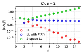
Figure 17: The coefficients of the series expansions for $\delta_{p}$, Eq. (96), using a variety of approximation for $\Sigma$, Eqs. (93)–(95), normalised to the coefficients from the DL series. The four plots show different combinations of colour factor and $p$. Circles with a central plus indicate a positive ratio, circles with a central dot indicate a negative ratio.

For each of the above approximations for $\Sigma(L)$, we can evaluate the impact of a $p_{t}^{p}$ dependence of the acceptance on the fiducial cross section, as

$$\delta_{p}\equiv\frac{\sigma_{\text{fid}}}{f_{0}\sigma_{\text{tot}}}-1=f_{p}\int_{0}^{\infty}dL\,e^{-pL}\partial_{L}\Sigma(L)=\sum_{n=1}^{\infty}\alpha_{s}^{n}c_{n}\,.$$ (96)

Fig. 17 shows the ratio of the $c_{n}$ as obtained with each of Eqs. (93)–(95) to the DL result for $c_{n}$. A first observation is that in all cases, asymptotically, the DL coefficients appear to be effectively rescaled by a factor $1/r^{n}$

$$c_{n}\sim\frac{c_{n}^{\text{\sc dl}}}{r^{n}}\,,$$ (97)

where $r$ is some constant. Below, we will consider how such a rescaling can come about. For now, however, we examine what we can learn from Fig. 17.

A first point is that with a modification of the series as in Eq. (97), the expression for the perturbative order at which one finds the smallest term in the perturbative series becomes

$$n_{\min}\simeq|r|\frac{\pi p^{2}}{8\alpha_{s}C}\,.$$ (98)

The effective power scaling of the minimal term in the series becomes

$$\left(\frac{\Lambda}{Q}\right)^{|r|\frac{(11C_{A}-2n_{f})p^{2}}{48C}}\,.$$ (99)

For $p=1$ (the upper row of Fig. 17) the LL, LL_F and LL_b results all yield compatible values of $r$. Specifically for the $p=1$, $C_{A}$ case we find $r\simeq 1.28$, corresponding to an effective power of $(\Lambda/Q)^{0.205}$. For the $p=1$, $C_{F}$ case we find $r\simeq 2.1$, corresponding to an effective power of $(\Lambda/Q)^{0.76}$. The agreement between the different approximations for $\Sigma$ suggests that the resulting rescaling factors and effective powers have a good chance of being representative of the actual asymptotic structure of the perturbative series.

In contrast, for $p=2$, we find that the LL, LL_F and LL_b approximations yield quite different results. We believe that the underlying reason is that the DL $p=2$ factorial growth is weaker than for $p=1$, and so there is a greater chance that artefacts of the various approximations for $\Sigma$ can more easily come to dominate the expansion. Specifically, the LL_F approximation has a well-known spurious all-order divergence for $R^{\prime}=2$, and integrating over the expansion of such a divergence is bound to generate (spurious, same-sign) factorial growth (careful investigation of Fig. 17 shows that $r$ is negative, i.e. the observed factorial growth is indeed of the same-sign variety). The approach of Ref. Monni:2016ktx offers ways of working around this issue, though the expansion of that approach to high perturbative orders would require further work. Meanwhile the LL_b approximation is known to generate spurious factorial growth in the coefficients of the distribution at finite $p_{t}$ Frixione:1998dw , a feature that we have explicitly confirmed by integrating over a region of moderate $L$. As a result, we believe that it is unlikely that the stronger-than-DL factorial growth seen with the $b$-space approach will be a genuine feature of the true perturbative series. Note that the modified logarithms used in Ref. Bozzi:2005wk may well address this problem, but they bring more complicated expansion expressions at high orders. Overall the conclusion is that to obtain a reliable understanding the asymptotics of the perturbative series for the $p=2$ case, further more careful work is needed.

As a final point, we examine analytically how a rescaling such as Eq. (97) can arise. Consider the coefficient of a term $\alpha_{s}^{n}L^{2n-\ell}$. For $\ell=0$, the coefficient scales as $1/n!$, which is promoted to $(2n)!/n!$ after the integration in Eq. (96). Naively one might expect terms with $\ell>0$ to be suppressed because the integration over $L$ will only give an enhancement $(2n-\ell)!$. However this assumes that the coefficient of $\alpha_{s}^{n}L^{2n-\ell}$ has the same factorial scaling as that of $\alpha_{s}^{n}L^{2n}$. To see why this is not the case, we supplement the DL approximation with just the term in the series expansion of $r_{1}(\lambda)$ in Eq. (93) that is proportional to $b_{0}$ (and its exponentiation), i.e. we consider the DL formula with the replacement

$$\frac{2C\alpha_{s}L^{2}}{\pi}\to\frac{2C\alpha_{s}L^{2}}{\pi}\left(1+\frac{4}{3}\alpha_{s}b_{0}L\right)\,.$$ (100)

Exponentiating this, after some straightforward manipulation, one obtains

$$\Sigma=\sum_{n=0}^{\infty}\frac{1}{n!}\left(-\frac{2C\alpha_{s}}{\pi}\right)^{n}\sum_{\ell=0}^{n/2}\frac{n!}{\ell!(n-2\ell)!}\left(-\frac{2\pi}{3}\frac{b_{0}}{C}\right)^{\ell}L^{2n-\ell}\,.$$ (101)

The result for $\delta_{p}$ is then

$$\delta_{p}=\frac{1}{2^{p}}\sum_{n=0}^{\infty}\frac{(2n)!}{n!}\left(-\frac{2C\alpha_{s}}{\pi p^{2}}\right)^{n}\sum_{\ell=0}^{n/2}\frac{1}{\ell!}\frac{n!}{(n-2\ell)!}\frac{(2n-\ell)!}{(2n)!}\left(-\frac{2\pi}{3}\frac{pb_{0}}{C}\right)^{\ell}\,.$$ (102)

Next we observe that when $n\gg\ell$,

$$\frac{n!}{(n-2\ell)!}\frac{(2n-\ell)!}{(2n)!}\simeq\frac{n^{2\ell}}{(2n)^{\ell}}=\left(\frac{n}{2}\right)^{\ell}\,,$$ (103)

from which we obtain

$$\delta_{p} \simeq\frac{1}{2^{p}}\sum_{n=0}^{\infty}\frac{(2n)!}{n!}\left(-\frac{2C\alpha_{s}}{\pi p^{2}}\right)^{n}\sum_{\ell=0}^{n/2}\frac{1}{\ell!}\left(-\frac{n\pi}{3}\frac{pb_{0}}{C}\right)^{\ell}\,,$$ (104a)

$$\simeq\frac{1}{2^{p}}\sum_{k=0}^{\infty}\frac{(2k)!}{k!}\left(-\frac{2C\alpha_{s}}{\pi p^{2}}\right)^{k}\exp\left(-\frac{k\pi}{3}\frac{pb_{0}}{C}\right)\,,$$ (104b)

which is precisely of the form of Eq. (97) with

$$r=\exp\left(\frac{\pi}{3}\frac{pb_{0}}{C}\right)\,.$$ (105)

For $p=1$ and $C=C_{A}$ this gives $r\simeq 1.24$, which is in the same ballpark as the complete numerical result given above of $r\simeq 1.28$. For $p=1$ and $C=C_{F}$, one finds $r\simeq 1.6$, which is not so close to the observed numerical result of $r=2.1$. In both cases, however, we have made quite a number of approximations, such as taking just the first non-trivial $b_{0}$ term as our starting point, Eq. (100), so it is perhaps unsurprising that the analysis does not yield the full structure of the series. Still, we believe that the analysis is sufficient to motivate the observed structural form of the scaling as written in Eq. (97) and observed in Fig. 17.

Appendix D Remarks on defiducialisation

An alternative approach to the elimination of artefacts from cuts is to adopt a defiducialisation procedure Glazov:2020gza . In the case of Higgs production and decay, this is particularly simple and one may write a defiducialised cross section as

$$\sigma_{\text{defid}} =\int_{-y_{\text{\sc h}}^{\text{max}}}^{+y_{\text{\sc h}}^{\text{max}}}dy_{\text{\sc h}}\int_{0}^{p_{t,\text{\sc h}}^{\text{max}}}dp_{t,\text{\sc h}}\frac{d\sigma^{\text{fid}}}{dy_{\text{\sc h}}dp_{t,\text{\sc h}}}\frac{1}{f(y_{\text{\sc h}},p_{t,\text{\sc h}})}\,,$$ (106a)

$$\equiv\int_{-y_{\text{\sc h}}^{\text{max}}}^{+y_{\text{\sc h}}^{\text{max}}}dy_{\text{\sc h}}\int_{0}^{p_{t,\text{\sc h}}^{\text{max}}}dp_{t,\text{\sc h}}\frac{d\sigma}{dy_{\text{\sc h}}dp_{t,\text{\sc h}}}\,,$$ (106b)

where $d\sigma^{\text{fid}}/{dy_{\text{\sc h}}dp_{t,\text{\sc h}}}$ is the differential cross section with some specific set of fiducial cuts, and $f(y_{\text{\sc h}},p_{t,\text{\sc h}}$) is the acceptance with those cuts. The meaning of Eq. (106a) is that each event that passes the cuts is binned with a weight $1/f(y_{\text{\sc h}},p_{t,\text{\sc h}})$. Such an approach effectively yields a bin of a simplified template cross section Berger:2019wnu , as made evident from Eq. (106b). Care is needed with the choice of $y_{\text{\sc h}}^{\text{max}}$ and $p_{t,\text{\sc h}}^{\text{max}}$ so as to avoid regions where the acceptance is zero or close to zero. This implies that that $y_{\text{\sc h}}^{\text{max}}$ should be kept well away from the upper limit on the photon acceptance (for example, for a maximum photon pseudorapidity of $2.37$, one might choose $y_{\text{\sc h}}^{\text{max}}=2$). With cuts that remove slices of (pseudo)rapidity for the photons, a $p_{t,\text{\sc h}}^{\text{max}}$ restriction may be necessary to avoid the high-$p_{t,\text{\sc h}}$ region where one or other of the photons from the Higgs decay is highly likely to be collimated into the slice. Alternatively, one may remove the slice regions from the rapidity integral.

To evaluate Eq. (106a) in practice, $f(y_{\text{\sc h}},p_{t,\text{\sc h}})$ can be pre-tabulated. If this is considered too cumbersome, one could instead evaluate

$$\sigma_{\text{defid}}=\int_{-y_{\text{\sc h}}^{\text{max}}}^{+y_{\text{\sc h}}^{\text{max}}}dy_{\text{\sc h}}\int_{0}^{p_{t,\text{\sc h}}^{\text{max}}}dp_{t,\text{\sc h}}\int d\phi_{\text{\sc cs}}\frac{d\sigma^{\text{fid}}}{dy_{\text{\sc h}}dp_{t,\text{\sc h}}d\phi_{\text{\sc cs}}}\left[\frac{1}{4}\sum_{i=1}^{4}f(y_{\text{\sc h}},p_{t,\text{\sc h}},\phi_{i})\right]^{-1}\,.$$ (107)

This equation is to be interpreted as follows: for each event, one determines $y_{\text{\sc h}}$, $p_{t,\text{\sc h}}$ and the Collins-Soper azimuth $\phi_{\text{\sc cs}}$. One then evaluates the quantity in square brackets across the four $\phi_{i}$ values as given in Eq. (71) and uses this to determine the weight when binning the event. The logic of this approach is that the quantity $f(y_{\text{\sc h}},p_{t,\text{\sc h}},\phi_{i})$ can be evaluated exactly, and relatively efficiently, with the help of the code supplied with this article. The sum over four $\phi_{i}$ values serves to avoid large fluctuations in event weights (for example due to the region of low $\phi_{\text{\sc cs}}$ values in the right-hand, $p_{t,\text{\sc h}}=100\;\mathrm{GeV}$, panel of Fig. 11, where the non-negotiable $p_{t,-}$ cut causes the acceptance to be very close to zero).

A further variant is to defiducialise just the $p_{t,\text{\sc h}}$ dependence. In our view, the simplest such approach is the following,

$$\sigma_{\text{defid},p_{t,\text{\sc h}}} =\int_{-y_{\text{\sc h}}^{\text{max}}}^{+y_{\text{\sc h}}^{\text{max}}}dy_{\text{\sc h}}\int_{0}^{p_{t,\text{\sc h}}^{\text{max}}}dp_{t,\text{\sc h}}\frac{d\sigma^{\text{fid}}}{dy_{\text{\sc h}}dp_{t,\text{\sc h}}}\frac{f(y_{\text{\sc h}},0)}{f(y_{\text{\sc h}},p_{t,\text{\sc h}})}\,,$$ (108a)

$$\equiv\int_{-y_{\text{\sc h}}^{\text{max}}}^{+y_{\text{\sc h}}^{\text{max}}}dy_{\text{\sc h}}\int_{0}^{p_{t,\text{\sc h}}^{\text{max}}}dp_{t,\text{\sc h}}\frac{d\sigma}{dy_{\text{\sc h}}dp_{t,\text{\sc h}}}f(y_{\text{\sc h}},0)\,,$$ (108b)

where the weight assigned to each observed event is now $\frac{f(y_{\text{\sc h}},0)}{f(y_{\text{\sc h}},p_{t,\text{\sc h}})}$. As with full defiducialisation, this may also be adapted to use a weight that is $\phi$-dependent.

Note that defiducialisation is a rigorous and straightforward procedure only for scalar decays. Applications to vector-boson decays (as in the original proposal) encounter the complication the angular distribution of the decay products depends on the kinematics and production mechanism of the vector boson in a non-trivial manner. One might consider exploring an approximate defiducialisation, e.g. based just on the unpolarised acceptance, however it is not clear to what extent this would be superior to the simple use of product cuts.

References

- (1) M. Klasen and G. Kramer, Dijet cross-sections at in photon–proton collisions, Phys. Lett. B 366 (1996) 385 [hep-ph/9508337].
- (2) B.W. Harris and J.F. Owens, Photoproduction of jets at HERA in next-to-leading order QCD, Phys. Rev. D 56 (1997) 4007 [hep-ph/9704324].
- (3) S. Frixione and G. Ridolfi, Jet photoproduction at HERA, Nucl. Phys. B 507 (1997) 315 [hep-ph/9707345].
- (4) G. Heinrich, Collider Physics at the Precision Frontier, Phys. Rept. 922 (2021) 1 [2009.00516].
- (5) C. Anastasiou, C. Duhr, F. Dulat, F. Herzog and B. Mistlberger, Higgs Boson Gluon-Fusion Production in QCD at Three Loops, Phys. Rev. Lett. 114 (2015) 212001 [1503.06056].
- (6) C. Anastasiou, C. Duhr, F. Dulat, E. Furlan, T. Gehrmann, F. Herzog et al., High precision determination of the gluon fusion Higgs boson cross-section at the LHC, JHEP 05 (2016) 058 [1602.00695].
- (7) C. Duhr, F. Dulat and B. Mistlberger, Drell-Yan Cross Section to Third Order in the Strong Coupling Constant, Phys. Rev. Lett. 125 (2020) 172001 [2001.07717].
- (8) C. Duhr, F. Dulat and B. Mistlberger, Charged current Drell-Yan production at N3LO, JHEP 11 (2020) 143 [2007.13313].
- (9) F. Dulat, B. Mistlberger and A. Pelloni, Precision predictions at N3LO for the Higgs boson rapidity distribution at the LHC, Phys. Rev. D 99 (2019) 034004 [1810.09462].
- (10) L. Cieri, X. Chen, T. Gehrmann, E.W.N. Glover and A. Huss, Higgs boson production at the LHC using the subtraction formalism at N3LO QCD, JHEP 02 (2019) 096 [1807.11501].
- (11) X. Chen, T. Gehrmann, E.W.N. Glover, A. Huss, B. Mistlberger and A. Pelloni, Fully Differential Higgs Boson Production to Third Order in QCD, 2102.07607.
- (12) G. Billis, B. Dehnadi, M.A. Ebert, J.K.L. Michel and F.J. Tackmann, The Higgs Spectrum and Total Cross Section with Fiducial Cuts at N3LL′+N3LO, 2102.08039.
- (13) S. Camarda, L. Cieri and G. Ferrera, Drell-Yan lepton-pair production: resummation at N3LL accuracy and fiducial cross sections at N3LO, 2103.04974.
- (14) S. Alekhin, A. Kardos, S. Moch and Z. Trócsányi, Precision studies for Drell-Yan processes at NNLO, 2104.02400.
- (15) M.A. Ebert and F.J. Tackmann, Impact of isolation and fiducial cuts on qT and N-jettiness subtractions, JHEP 03 (2020) 158 [1911.08486].
- (16) M.A. Ebert, J.K.L. Michel, I.W. Stewart and F.J. Tackmann, Drell-Yan resummation of fiducial power corrections at N3LL, JHEP 04 (2021) 102 [2006.11382].
- (17) M. Beneke, Renormalons, Phys. Rept. 317 (1999) 1 [hep-ph/9807443].
- (18) M. Beneke and V.M. Braun, Power corrections and renormalons in Drell-Yan production, Nucl. Phys. B 454 (1995) 253 [hep-ph/9506452].
- (19) M. Dasgupta, Power corrections to the differential Drell-Yan cross-section, JHEP 12 (1999) 008 [hep-ph/9911391].
- (20) S. Ferrario Ravasio, G. Limatola and P. Nason, Infrared renormalons in kinematic distributions for hadron collider processes, JHEP 06 (2021) 018 [2011.14114].
- (21) F. Caola, S.F. Ravasio, G. Limatola, K. Melnikov and P. Nason, On linear power corrections in certain collider observables, 2108.08897.
- (22) A. Banfi and M. Dasgupta, Dijet rates with symmetric cuts, JHEP 01 (2004) 027 [hep-ph/0312108].
- (23) M. Dasgupta, F.A. Dreyer, K. Hamilton, P.F. Monni, G.P. Salam and G. Soyez, Parton showers beyond leading logarithmic accuracy, Phys. Rev. Lett. 125 (2020) 052002 [2002.11114].
- (24) K. Hamilton, R. Medves, G.P. Salam, L. Scyboz and G. Soyez, Colour and logarithmic accuracy in final-state parton showers, 2011.10054.
- (25) A. Karlberg, G.P. Salam, L. Scyboz and R. Verheyen, Spin correlations in final-state parton showers and jet observables, 2103.16526.
- (26) J.R. Forshaw, J. Holguin and S. Plätzer, Building a consistent parton shower, JHEP 09 (2020) 014 [2003.06400].
- (27) J. Holguin, J.R. Forshaw and S. Plätzer, Improvements on dipole shower colour, Eur. Phys. J. C 81 (2021) 364 [2011.15087].
- (28) Z. Nagy and D.E. Soper, Summations by parton showers of large logarithms in electron-positron annihilation, 2011.04777.
- (29) Z. Nagy and D.E. Soper, Summations of large logarithms by parton showers, 2011.04773.
- (30) P.F. Monni, P. Nason, E. Re, M. Wiesemann and G. Zanderighi, MiNNLOPS: a new method to match NNLO QCD to parton showers, JHEP 05 (2020) 143 [1908.06987].
- (31) S. Alioli, A. Broggio, A. Gavardi, S. Kallweit, M.A. Lim, R. Nagar et al., Matching NNLO to parton shower using N3LL colour-singlet transverse momentum resummation in GENEVA, 2102.08390.
- (32) S. Prestel, Matching N3LO QCD calculations to parton showers, 2106.03206.
- (33) A. Glazov, Defiducialization: Providing Experimental Measurements for Accurate Fixed-Order Predictions, Eur. Phys. J. C 80 (2020) 875 [2001.02933].
- (34) H1 collaboration, Dijet event rates in deep inelastic scattering at HERA, Eur. Phys. J. C 13 (2000) 415 [hep-ex/9806029].
- (35) T. Carli, Renormalization scale dependencies in dijet production at HERA, in Workshop on Monte Carlo Generators for HERA Physics (Plenary Starting Meeting), 4, 1998 [hep-ph/9906541].
- (36) H1 collaboration, Measurement and QCD analysis of jet cross-sections in deep inelastic positron - proton collisions at s**(1/2) of 300-GeV, Eur. Phys. J. C 19 (2001) 289 [hep-ex/0010054].
- (37) M. Rubin, G.P. Salam and S. Sapeta, Giant QCD K-factors beyond NLO, JHEP 09 (2010) 084 [1006.2144].
- (38) N. Berger et al., Simplified Template Cross Sections - Stage 1.1, 1906.02754.
- (39) F. Bishara, U. Haisch, P.F. Monni and E. Re, Constraining Light-Quark Yukawa Couplings from Higgs Distributions, Phys. Rev. Lett. 118 (2017) 121801 [1606.09253].
- (40) Y. Soreq, H.X. Zhu and J. Zupan, Light quark Yukawa couplings from Higgs kinematics, JHEP 12 (2016) 045 [1606.09621].
- (41) J.C. Collins and D.E. Soper, Angular Distribution of Dileptons in High-Energy Hadron Collisions, Phys. Rev. D 16 (1977) 2219.
- (42) ATLAS collaboration, Measurements of Higgs boson properties in the diphoton decay channel with 36 fb-1 of collision data at TeV with the ATLAS detector, Phys. Rev. D98 (2018) 052005 [1802.04146].
- (43) G. Parisi and R. Petronzio, Small Transverse Momentum Distributions in Hard Processes, Nucl. Phys. B 154 (1979) 427.
- (44) P.F. Monni, E. Re and P. Torrielli, Higgs Transverse-Momentum Resummation in Direct Space, Phys. Rev. Lett. 116 (2016) 242001 [1604.02191].
- (45) W. Bizon, P.F. Monni, E. Re, L. Rottoli and P. Torrielli, Momentum-space resummation for transverse observables and the Higgs p⟂ at N3LL+NNLO, JHEP 02 (2018) 108 [1705.09127].
- (46) W. Bizoń, X. Chen, A. Gehrmann-De Ridder, T. Gehrmann, N. Glover, A. Huss et al., Fiducial distributions in Higgs and Drell-Yan production at N3LL+NNLO, JHEP 12 (2018) 132 [1805.05916].
- (47) J. Butterworth et al., PDF4LHC recommendations for LHC Run II, J. Phys. G 43 (2016) 023001 [1510.03865].
- (48) I. Scimemi and A. Vladimirov, Non-perturbative structure of semi-inclusive deep-inelastic and Drell-Yan scattering at small transverse momentum, JHEP 06 (2020) 137 [1912.06532].
- (49) A. Bacchetta, V. Bertone, C. Bissolotti, G. Bozzi, F. Delcarro, F. Piacenza et al., Transverse-momentum-dependent parton distributions up to N3LL from Drell-Yan data, JHEP 07 (2020) 117 [1912.07550].
- (50) T. Becher and T. Neumann, Fiducial resummation of color-singlet processes at N3LL+NNLO, JHEP 03 (2021) 199 [2009.11437].
- (51) E. Re, L. Rottoli and P. Torrielli, Fiducial Higgs and Drell-Yan distributions at N3LL′+NNLO with RadISH, 2104.07509.
- (52) M.A. Ebert, I. Moult, I.W. Stewart, F.J. Tackmann, G. Vita and H.X. Zhu, Subleading power rapidity divergences and power corrections for qT, JHEP 04 (2019) 123 [1812.08189].
- (53) M. Cacciari, F.A. Dreyer, A. Karlberg, G.P. Salam and G. Zanderighi, Fully Differential Vector-Boson-Fusion Higgs Production at Next-to-Next-to-Leading Order, Phys. Rev. Lett. 115 (2015) 082002 [1506.02660].
- (54) D0 collaboration, Measurement of the electron charge asymmetry in decays in collisions at TeV, Phys. Rev. D 91 (2015) 032007 [1412.2862].
- (55) CMS collaboration, Measurements of the boson rapidity, helicity, double-differential cross sections, and charge asymmetry in collisions at = 13 TeV, Phys. Rev. D 102 (2020) 092012 [2008.04174].
- (56) Sherpa collaboration, Event Generation with Sherpa 2.2, SciPost Phys. 7 (2019) 034 [1905.09127].
- (57) CMS collaboration, Measurement of inclusive and differential Higgs boson production cross sections in the diphoton decay channel in proton-proton collisions at 13 TeV, JHEP 01 (2019) 183 [1807.03825].
- (58) ATLAS collaboration, Measurements and interpretations of Higgs-boson fiducial cross sections in the diphoton decay channel using 139 of collision data at = 13 TeV with the ATLAS detector, Tech. Rep. ATLAS-CONF-2019-029 (7, 2019).
- (59) M. Cacciari, G.P. Salam and G. Soyez, FastJet User Manual, Eur. Phys. J. C 72 (2012) 1896 [1111.6097].
- (60) L.A. Harland-Lang, M. Tasevsky, V.A. Khoze and M.G. Ryskin, A new approach to modelling elastic and inelastic photon-initiated production at the LHC: SuperChic 4, Eur. Phys. J. C 80 (2020) 925 [2007.12704].
- (61) A. Denner, S. Dittmaier, T. Kasprzik and A. Muck, Electroweak corrections to dilepton + jet production at hadron colliders, JHEP 06 (2011) 069 [1103.0914].
- (62) R. Frederix and T. Vitos, Electroweak corrections to the angular coefficients in finite- Z-boson production and dilepton decay, Eur. Phys. J. C 80 (2020) 939 [2007.08867].
- (63) R. Gauld, A. Gehrmann-De Ridder, T. Gehrmann, E.W.N. Glover and A. Huss, Precise predictions for the angular coefficients in Z-boson production at the LHC, JHEP 11 (2017) 003 [1708.00008].
- (64) J.C. Collins, Simple Prediction of QCD for Angular Distribution of Dileptons in Hadron Collisions, Phys. Rev. Lett. 42 (1979) 291.
- (65) D. Boer and W. Vogelsang, Drell-Yan lepton angular distribution at small transverse momentum, Phys. Rev. D 74 (2006) 014004 [hep-ph/0604177].
- (66) E.L. Berger, J.-W. Qiu and R.A. Rodriguez-Pedraza, Angular distribution of leptons from the decay of massive vector bosons, Phys. Lett. B 656 (2007) 74 [0707.3150].
- (67) A. Bodek, A simple event weighting technique for optimizing the measurement of the forward-backward asymmetry of Drell-Yan dilepton pairs at hadron colliders, Eur. Phys. J. C 67 (2010) 321 [0911.2850].
- (68) J. Lindfors, Angular Distribution of Large -transverse Muon Pairs in Different Reference Frames, Phys. Scripta 20 (1979) 19.
- (69) CMS collaboration, Measurements of differential Z boson production cross sections in proton-proton collisions at = 13 TeV, JHEP 12 (2019) 061 [1909.04133].
- (70) S. Catani and M. Grazzini, An NNLO subtraction formalism in hadron collisions and its application to Higgs boson production at the LHC, Phys. Rev. Lett. 98 (2007) 222002 [hep-ph/0703012].
- (71) S. Frixione, P. Nason and G. Ridolfi, Problems in the resummation of soft gluon effects in the transverse momentum distributions of massive vector bosons in hadronic collisions, Nucl. Phys. B 542 (1999) 311 [hep-ph/9809367].
- (72) A. Kulesza and W.J. Stirling, Soft gluon resummation in transverse momentum space for electroweak boson production at hadron colliders, Eur. Phys. J. C 20 (2001) 349 [hep-ph/0103089].
- (73) G. Bozzi, S. Catani, D. de Florian and M. Grazzini, Transverse-momentum resummation and the spectrum of the Higgs boson at the LHC, Nucl. Phys. B 737 (2006) 73 [hep-ph/0508068].