Theory of unidirectional magnetoresistance and nonlinear Hall effect

Abstract

We study the unidirectional magnetoresistance (UMR) and the nonlinear Hall effect (NLHE) in the ferromagnetic Rashba model. For this purpose we derive expressions to describe the response of the electric current quadratic in the applied electric field. We compare two different formalisms, namely the standard Keldysh nonequilibrium formalism and the Moyal-Keldysh formalism, to derive the nonlinear conductivities of UMR and NLHE. We find that both formalisms lead to identical numerical results when applied to the ferromagnetic Rashba model. The UMR and the NLHE nonlinear conductivities tend to be comparable in magnitude according to our calculations. Additionally, their dependencies on the Rashba parameter and on the quasiparticle broadening are similar. The nonlinear zero-frequency response considered here is several orders of magnitude higher than the one at optical frequencies that describes the photocurrent generation in the ferromagnetic Rashba model. Additionally, we compare our Keldysh nonequilibrium expression in the independent-particle approximation to literature expressions of the UMR that have been obtained within the constant relaxation time approximation of the Boltzmann formalism. We find that both formalisms converge to the same analytical formula in the limit of infinite relaxation time. However, remarkably, we find that the Boltzmann result does not correspond to the intraband term of the Keldysh expression. Instead, the Boltzmann result corresponds to the sum of the intraband term and an interband term that can be brought into the form of an effective intraband term due to the f-sum rule.

I Introduction

In magnetic bilayers such as Co/Pt, which are composed of a ferromagnetic layer and a heavy metal layer, a change in the longitudinal resistance is observed when either the applied in-plane current or the magnetization is reversed [1, 2, 3]. This so-called unidirectional magnetoresistance (UMR) is proportional to $({\boldsymbol{j}}\times\hat{{\boldsymbol{e}}}_{z})\cdot\hat{{\boldsymbol{M}}}$, where ${\boldsymbol{j}}$, $\hat{{\boldsymbol{M}}}$, and $\hat{{\boldsymbol{e}}}_{z}$ denote the electric current, the magnetization direction, and the unit vector along the bilayer interface normal, respectively. UMR is a nonlinear magnetoresistance, because the corresponding voltage is quadratic in the applied electric current. Therefore, UMR generates a 2nd harmonic voltage when an a.c. current is applied. UMR can be used to detect 180^∘ magnetization reversal [4, 5] and to realize reversible diodes [6]. Using UMR the four different magnetic states that may be realized in ferromagnet/nonmagnet/ferromagnet trilayers may be differentiated [5].

One contribution to the UMR arises from spin accumulation in the ferromagnetic layer, which modifies the electrical conductivity when the mobility is spin-dependent [6]. The spin accumulation itself may arise from the spin Hall effect (SHE) in the heavy metal, which injects spin current into the ferromagnet. Additionally, the interfacial spin accumulation may modify the interface contribution to the conductivity, which may contribute to the UMR as well [7]. A thickness-dependent study [8] in magnetic bilayers confirms the role of the SHE for the UMR. Another indication that the SHE is very often at the heart of the UMR in metallic bilayers comes from the observation that the UMR correlates with the antidamping spin-orbit torque, but not with the field-like one [1]. This picture changes if Rashba interface states dominate the interfacial magnetotransport properties: In Fe/Ge(111) a large UMR has been found that has been attributed to the Rashba effect of the interface states [9]. Also in heterostructures composed of a topological insulator on a ferromagnet the Rashba-Edelstein effect has been found to contribute to the UMR as well [10].

Moreover, the spin current injected into the ferromagnet due to the SHE of the heavy metal layer may excite magnons in the ferromagnet. These magnons may modify the resistivity of the ferromagnetic layer similarly to the spin-disorder contribution to the resistivity and thus contribute to the UMR [7]. The large UMR in topological insulator heterostructures has been attributed to asymmetric electron-magnon scattering [11]. Finally, UMR exists not only in magnetic heterostructures but also in bulk ferromagnets with broken inversion symmetry [4, 12], which might require different models to describe the UMR than the heterostructures.

In addition to the UMR the nonlinear response to the applied electric current contains also the nonlinear Hall effect (NLHE) [13]. Some mechanisms of the UMR discussed above may also lead to NLHE. For example, asymmetric electron-magnon scattering has been found to contribute to the NLHE [14].

So far, most theoretical models of UMR address only one particular mechanism. Ref. [6] develops a model to describe the UMR from the modulation of the conductivity of the ferromagnetic layer when a spin current from a heavy metal layer is injected due to the SHE. For magnetic bilayer systems composed of an insulating ferromagnet on a heavy metal layer a theoretical model was developed to describe the magnonic contribution to the UMR [15]. Ref. [12] uses the Boltzmann transport theory to derive an expression for UMR, which is applied to NiMnSb. Ref. [16] expresses the nonlinear conductivity in the clean limit in terms of the Berry curvature dipole and a Drude term and applies this theory to a model of BaMn₂As₂.

While UMR and NLHE are relatively new effects in spintronics, there are much older second order responses well-known in nonlinear optics, e.g. the shift current, the injection current and the 2nd harmonic generation [17]. The nonlinear conductivities at optical frequencies contain also the photovoltaic anomalous Hall effect, which has been considered recently in line-node semimetals [18], and it also contains the photovoltaic chiral magnetic effect, which has been studied in Weyl semimetals recently [19]. At first glance it is tempting to guess that formulae suitable to compute the UMR and the NLHE may be obtained easily by taking the zero-frequency limit of the dc photocurrent expressions. However, as we will discuss in this work this is not the case. Nevertheless, it is instructive to compare the second order response tensors derived in nonlinear optics to the expressions for UMR and NLHE. Since second order response coefficients are considerably more complicated to compute than the linear ones a large number of nonlinear optics works are devoted to the topic of comparing various formalisms and finding the most efficient approach for calculations [17, 20, 21, 22, 23, 24]. An important conclusion of these works is that all formalisms yield the same answer if all caveats are considered properly.

In view of the large number of the proposed mechanisms of UMR and NLHE it is desirable to derive general expressions for the nonlinear response coefficients that quantify these effects. Ideally, these expressions should cover all possible mechanisms and they should be in a form that allows us to apply them within first-principles density-functional theory calculations. In this work we derive formulae for the second order response of the electric current to an applied electric field using two different approaches: The Keldysh nonequilibrium formalism on the one hand and the Moyal-Keldysh formalism on the other hand. We show that these two different formalisms lead to identical numerical results for the UMR and the NLHE in the ferromagnetic Rashba model, which corroborates the applicability of both methods to magnetic Hamiltonians with spin-orbit interaction (SOI). In our numerical study of the Rashba model we use the independent particle approximation and describe effects of disorder effectively through a quasiparticle broadening parameter. However, in our general presentation of the Moyal-Keldysh formalism we give explicit expressions for the self-energies, which may be used to go beyond this constant broadening model. In our discussion of the UMR and NLHE in the ferromagnetic Rashba model we investigate the dependence on the SOI strength, on the Fermi energy, and on the quasiparticle broadening. Additionally, we show analytically that the Keldysh approach converges to the same result as an expression in the literature that was obtained from the Boltzmann formalism within the constant relaxation time approximation.

This paper is structured as follows: In Sec. II.1 we use the Keldysh formalism to derive the response coefficient for the second order in the applied electric field. In Sec. II.2 we use the Moyal-Keldysh technique to derive this response, where we defer detailed definitions of Green functions and self energies to the Appendix A. In Sec. II.3 we introduce the ferromagnetic Rashba model, which we use for the numerical study of UMR and NLHE. In Sec. II.4 we discuss the symmetry properties of the UMR and the NLHE in the ferromagnetic Rashba model. In Sec. III we discuss the numerical results on the UMR and the NLHE that we obtain in the ferromagnetic Rashba model using our Keldysh and Moyal-Keldysh approaches. This paper ends with a summary in Sec. IV.

II Formalism

II.1 Keldysh formalism

We describe the action of the applied electric field through the time-dependent perturbation

$$\delta H(t)=e{\boldsymbol{v}}\cdot{\boldsymbol{A}}(t)$$ (1)

to the Hamiltonian $H$, where $e$ is the elementary positive charge, ${\boldsymbol{v}}$ is the velocity operator and

$${\boldsymbol{A}}(t)=\frac{1}{2}\left[\frac{{\boldsymbol{E}}_{0}e^{-i\omega t}}{i\omega}-\frac{{\boldsymbol{E}}_{0}e^{i\omega t}}{i\omega}\right]=-\frac{{\boldsymbol{E}}_{0}\sin(\omega t)}{\omega}$$ (2)

is the vector potential with the corresponding electric field

$${\boldsymbol{E}}(t)=-\frac{\partial{\boldsymbol{A}}(t)}{\partial t}=\frac{{\boldsymbol{E}}_{0}}{2}\left[e^{i\omega t}+e^{-i\omega t}\right]={\boldsymbol{E}}_{0}\cos(\omega t).$$ (3)

In the course of the following derivations we will take the limit frequency $\omega\rightarrow 0$ below in order to extract the dc response.

The electric current density is given by

$${\boldsymbol{j}}(t)=-\frac{e}{iV}{\rm Tr}\left[{\boldsymbol{v}}G^{<}(t,t)\right],$$ (4)

where $G^{<}$ is the lesser Green function and $V$ is the volume of the system. One may expand $G^{<}$ in orders of the perturbation $\delta H(t)$. The contribution to $G^{<}$ that is quadratic in $\delta H(t)$ is given by [25]

$$G^{<}_{2}(t,t^{\prime})=$$ (5)

$$\int\!\!{\rm d}t_{1}\!\!\int\!\!{\rm d}t_{2}\,G^{\rm R}_{\rm 0}(t,t_{1})\frac{\delta H(t_{1})}{\hbar}G^{\rm R}_{\rm 0}(t_{1},t_{2})\frac{\delta H(t_{2})}{\hbar}G^{<}_{\rm 0}(t_{2},t^{\prime})+$$

$$\int\!\!{\rm d}t_{1}\!\!\int\!\!{\rm d}t_{2}\,G^{\rm R}_{\rm 0}(t,t_{1})\frac{\delta H(t_{1})}{\hbar}G^{<}_{\rm 0}(t_{1},t_{2})\frac{\delta H(t_{2})}{\hbar}G_{\rm 0}^{\rm A}(t_{2},t^{\prime})+$$

$$\int\!\!{\rm d}t_{1}\!\!\int\!\!{\rm d}t_{2}\,G_{\rm 0}^{<}(t,t_{1})\frac{\delta H(t_{1})}{\hbar}G_{\rm 0}^{\rm A}(t_{1},t_{2})\frac{\delta H(t_{2})}{\hbar}G_{\rm 0}^{\rm A}(t_{2},t^{\prime}),$$

where

$$G^{\rm R}_{\rm 0}(t,t^{\prime})=\frac{1}{2\pi\hbar}\int_{-\infty}^{\infty}\!\!{\rm d}\mathcal{E}\,{\rm e}^{-i\mathcal{E}(t-t^{\prime})/\hbar}G^{\rm R}_{\rm 0}(\mathcal{E})$$ (6)

is the retarded Green function in equilibrium with Fourier transform $G^{\rm R}_{\rm 0}(\mathcal{E})=\hbar/[\mathcal{E}-H+i\Gamma]$. Similarly, $G^{\rm A}_{\rm 0}(t,t_{1})$ and $G^{<}_{\rm 0}(t,t_{1})$ are the advanced and lesser Green functions in equilibrium, respectively, with Fourier transforms $G^{\rm A}_{\rm 0}(\mathcal{E})=[G^{\rm R}_{\rm 0}(\mathcal{E})]^{\dagger}$ and $G^{<}_{\rm 0}(\mathcal{E})=[G^{\rm A}_{\rm 0}(\mathcal{E})-G^{\rm R}_{\rm 0}(\mathcal{E}))]f(\mathcal{E})$, where $f(\mathcal{E})$ is the Fermi-Dirac distribution function. In this section we use the independent particle approximation and assume that lifetime effects and effects of impurity scattering can be described by the quasiparticle broadening $\Gamma>0$. In section II.2 we will give explicit expressions to compute the self-energy within the Moyal-Keldysh approach.

In order to evaluate the time-integrations in Eq. (5) we use

$$\int\!\!\!{\rm d}t_{1}\!\!\!\int\!\!\!{\rm d}t_{2}G_{\rm 0}^{\eta}(t,t_{1})e^{-i\omega_{1}t_{1}}G_{\rm 0}^{\eta^{\prime}}(t_{1},t_{2})e^{-i\omega_{2}t_{2}}G_{\rm 0}^{\eta^{\prime\prime}}(t_{2},t)=$$ (7)

$$=\frac{{\rm e}^{-i[\omega_{1}+\omega_{2}]t}}{h}\!\int\!\!{\rm d}\mathcal{E}G_{\rm 0}^{\eta}(\mathcal{E}\!+\!\hbar\omega_{1})G_{\rm 0}^{\eta^{\prime}}(\mathcal{E})G_{\rm 0}^{\eta^{\prime\prime}}\!(\mathcal{E}\!-\!\hbar\omega_{2}),$$

where $\eta,\eta^{\prime},\eta^{\prime\prime}={\rm R,A,<}$ and $\omega_{1},\omega_{2}=\pm\omega$. When we set $\omega_{1}=\omega_{2}=\pm\omega$ we obtain the $2\omega$ and $-2\omega$ contributions, while we access the dc component by setting $\omega_{1}=-\omega_{2}=\pm\omega$. Thus, the $-2\omega$ component of the lesser Green function is given by

$$G^{<}_{-2\omega}(t,t)=-\frac{e^{2}}{4\omega^{2}h\hbar^{2}}\mathcal{F}(\omega,-\omega)e^{-2i\omega t},$$ (8)

where we defined

$$\mathcal{F}(\Omega_{1},\Omega_{2})=\int{\rm d}\mathcal{E}$$ (9)

$$G^{\rm R}_{0}(\mathcal{E}+\hbar\Omega_{1}){\boldsymbol{v}}\cdot{\boldsymbol{E}}_{0}G^{\rm R}_{0}(\mathcal{E}){\boldsymbol{v}}\cdot{\boldsymbol{E}}_{0}G^{<}_{0}(\mathcal{E}+\hbar\Omega_{2})+$$

$$+ G^{\rm R}_{0}(\mathcal{E}+\hbar\Omega_{1}){\boldsymbol{v}}\cdot{\boldsymbol{E}}_{0}G^{<}_{0}(\mathcal{E}){\boldsymbol{v}}\cdot{\boldsymbol{E}}_{0}G^{\rm A}_{0}(\mathcal{E}+\hbar\Omega_{2})+$$

$$+ G^{<}_{0}(\mathcal{E}+\hbar\Omega_{1}){\boldsymbol{v}}\cdot{\boldsymbol{E}}_{0}G^{\rm A}_{0}(\mathcal{E}){\boldsymbol{v}}\cdot{\boldsymbol{E}}_{0}G^{\rm A}_{0}(\mathcal{E}+\hbar\Omega_{2}).$$

Similarly, the $2\omega$ component is given by

$$G^{<}_{2\omega}(t,t)=-\frac{e^{2}}{4\omega^{2}h\hbar^{2}}\mathcal{F}(-\omega,\omega)e^{2i\omega t},$$ (10)

and the dc component is as follows:

$$G^{<}_{\rm dc}(t,t)=\frac{e^{2}}{4\omega^{2}h\hbar^{2}}\left[\mathcal{F}(-\omega,-\omega)+\mathcal{F}(\omega,\omega)\right].$$ (11)

Obviously, these three components may be written as products of the $\omega^{-2}$ factor, the complex exponential, and the remainder of the expression: $G^{<}_{-2\omega}(t,t)=\omega^{-2}g^{<}_{-2\omega}(\omega)e^{-2i\omega t}$, $G^{<}_{2\omega}(t,t)=\omega^{-2}g^{<}_{2\omega}(\omega)e^{2i\omega t}$, and $G^{<}_{\rm dc}(t,t)=\omega^{-2}g^{<}_{\rm dc}(\omega)$. The sum of these three contributions may thus be formulated as

$$[G^{<}_{-2\omega}(t,t)+G^{<}_{2\omega}(t,t)+G^{<}_{\rm dc}(t,t)]=$$ (12)

$$\frac{1}{\omega^{2}} [g^{<}_{-2\omega}(\omega)+g^{<}_{2\omega}(\omega)+g^{<}_{\rm dc}(\omega)]\cos^{2}(\omega t)+$$

$$+\frac{1}{\omega^{2}} [-g^{<}_{-2\omega}(\omega)-g^{<}_{2\omega}(\omega)+g^{<}_{\rm dc}(\omega)]\sin^{2}(\omega t)+$$

$$+\frac{i}{\omega^{2}} [-g^{<}_{-2\omega}(\omega)+g^{<}_{2\omega}(\omega)]\sin(2\omega t).$$

Next, we need to take the $\omega\rightarrow 0$ limit in order to extract the dc response. Since the dc response is time-independent by definition, we have the freedom to set $t$ in Eq. (12) to a value that makes the evaluation particularly convenient. Therefore, we choose $t=0$, because then only the first term on the right-hand side of Eq. (12) needs to be computed, because the second and third terms are zero for $t=0$:

$$[G^{<}_{-2\omega}(0,0)+G^{<}_{2\omega}(0,0)+G^{<}_{\rm dc}(0,0)]=$$ (13)

$$\frac{1}{\omega^{2}} [g^{<}_{-2\omega}(\omega)+g^{<}_{2\omega}(\omega)+g^{<}_{\rm dc}(\omega)].$$

In order to compute the zero-frequency limit of Eq. (13) we first observe that $\lim_{\omega\rightarrow 0}[g^{<}_{-2\omega}(\omega)+g^{<}_{2\omega}(\omega)+g^{<}_{\rm dc}(\omega)]=0$, because

$$\lim_{\omega\rightarrow 0}\left[-\mathcal{F}(\omega,-\omega)-\mathcal{F}(-\omega,\omega)+\mathcal{F}(-\omega,-\omega)+\mathcal{F}(\omega,\omega)\right]$$ (14)

$$=\left[-\mathcal{F}(0,0)-\mathcal{F}(0,0)+\mathcal{F}(0,0)+\mathcal{F}(0,0)\right]=0.$$

Moreover, we can show that

$$\lim_{\omega\rightarrow 0}\frac{1}{\omega}[g^{<}_{-2\omega}(\omega)+g^{<}_{2\omega}(\omega)+g^{<}_{\rm dc}(\omega)]=$$ (15)

$$= \lim_{\omega\rightarrow 0}\frac{\partial}{\partial\omega}[g^{<}_{-2\omega}(\omega)+g^{<}_{2\omega}(\omega)+g^{<}_{\rm dc}(\omega)]=0.$$

Consequently, we may use

$$\lim_{\omega\rightarrow 0}\frac{1}{\omega^{2}}[g^{<}_{-2\omega}(\omega)+g^{<}_{2\omega}(\omega)+g^{<}_{\rm dc}(\omega)]=$$ (16)

$$\lim_{\omega\rightarrow 0}\frac{1}{2}\frac{\partial^{2}}{\partial\omega^{2}}[g^{<}_{-2\omega}(\omega)+g^{<}_{2\omega}(\omega)+g^{<}_{\rm dc}(\omega)].$$

These zero-frequency limits of the second derivatives are given by

$$\lim_{\omega\rightarrow 0}\frac{1}{2}\frac{\partial^{2}}{\partial\omega^{2}}g^{<}_{2\omega}(\omega)=\lim_{\omega\rightarrow 0}\frac{1}{2}\frac{\partial^{2}}{\partial\omega^{2}}g^{<}_{-2\omega}(\omega)=-\Xi(-2)$$ (17)

and

$$\lim_{\omega\rightarrow 0}\frac{1}{2}\frac{\partial^{2}}{\partial\omega^{2}}g^{<}_{\rm dc}(\omega)=2\,\Xi(2),$$ (18)

where we defined the function

$$\Xi(\xi)=\frac{e^{2}}{8h}\int{\rm d}\mathcal{E}\Big{\{}$$ (19)

$$\frac{\partial^{2}}{\partial\mathcal{E}^{2}}G^{\rm R}_{0}(\mathcal{E}){\boldsymbol{v}}\cdot{\boldsymbol{E}}_{0}G^{\rm R}_{0}(\mathcal{E}){\boldsymbol{v}}\cdot{\boldsymbol{E}}_{0}G^{<}_{0}(\mathcal{E})+$$

$$G^{\rm R}_{0}(\mathcal{E}){\boldsymbol{v}}\cdot{\boldsymbol{E}}_{0}G^{\rm R}_{0}(\mathcal{E}){\boldsymbol{v}}\cdot{\boldsymbol{E}}_{0}\frac{\partial^{2}}{\partial\mathcal{E}^{2}}G^{<}_{0}(\mathcal{E})+$$

$$\xi\frac{\partial}{\partial\mathcal{E}}G^{\rm R}_{0}(\mathcal{E}){\boldsymbol{v}}\cdot{\boldsymbol{E}}_{0}G^{\rm R}_{0}(\mathcal{E}){\boldsymbol{v}}\cdot{\boldsymbol{E}}_{0}\frac{\partial}{\partial\mathcal{E}}G^{<}_{0}(\mathcal{E})+$$

$$+ \frac{\partial^{2}}{\partial\mathcal{E}^{2}}G^{\rm R}_{0}(\mathcal{E}){\boldsymbol{v}}\cdot{\boldsymbol{E}}_{0}G^{<}_{0}(\mathcal{E}){\boldsymbol{v}}\cdot{\boldsymbol{E}}_{0}G^{\rm A}_{0}(\mathcal{E})+$$

$$+ G^{\rm R}_{0}(\mathcal{E}){\boldsymbol{v}}\cdot{\boldsymbol{E}}_{0}G^{<}_{0}(\mathcal{E}){\boldsymbol{v}}\cdot{\boldsymbol{E}}_{0}\frac{\partial^{2}}{\partial\mathcal{E}^{2}}G^{\rm A}_{0}(\mathcal{E})+$$

$$\xi\frac{\partial}{\partial\mathcal{E}}G^{\rm R}_{0}(\mathcal{E}){\boldsymbol{v}}\cdot{\boldsymbol{E}}_{0}G^{<}_{0}(\mathcal{E}){\boldsymbol{v}}\cdot{\boldsymbol{E}}_{0}\frac{\partial}{\partial\mathcal{E}}G^{\rm A}_{0}(\mathcal{E})+$$

$$+ \frac{\partial^{2}}{\partial\mathcal{E}^{2}}G_{0}^{<}(\mathcal{E}){\boldsymbol{v}}\cdot{\boldsymbol{E}}_{0}G^{\rm A}_{0}(\mathcal{E}){\boldsymbol{v}}\cdot{\boldsymbol{E}}_{0}G^{\rm A}_{0}(\mathcal{E})+$$

$$+ G_{0}^{<}(\mathcal{E}){\boldsymbol{v}}\cdot{\boldsymbol{E}}_{0}G^{\rm A}_{0}(\mathcal{E}){\boldsymbol{v}}\cdot{\boldsymbol{E}}_{0}\frac{\partial^{2}}{\partial\mathcal{E}^{2}}G^{\rm A}_{0}(\mathcal{E})+$$

$$+ \xi\frac{\partial}{\partial\mathcal{E}}G_{0}^{<}(\mathcal{E}){\boldsymbol{v}}\cdot{\boldsymbol{E}}_{0}G^{\rm A}_{0}(\mathcal{E}){\boldsymbol{v}}\cdot{\boldsymbol{E}}_{0}\frac{\partial}{\partial\mathcal{E}}G^{\rm A}_{0}(\mathcal{E})\Big{\}}.$$

Summing up terms, we obtain

$$\lim_{\omega\rightarrow 0}\frac{g^{<}_{-2\omega}(\omega)+g^{<}_{2\omega}(\omega)+g^{<}_{\rm dc}(\omega)}{\omega^{2}}=\frac{e^{2}}{2h}\int{\rm d}\mathcal{E}\Big{\{}$$ (20)

$$2\frac{\partial}{\partial\mathcal{E}}G^{\rm R}_{0}(\mathcal{E}){\boldsymbol{v}}\cdot{\boldsymbol{E}}_{0}G^{\rm R}_{0}(\mathcal{E}){\boldsymbol{v}}\cdot{\boldsymbol{E}}_{0}\frac{\partial}{\partial\mathcal{E}}G^{<}_{0}(\mathcal{E})+$$

$$2\frac{\partial}{\partial\mathcal{E}}G^{\rm R}_{0}(\mathcal{E}){\boldsymbol{v}}\cdot{\boldsymbol{E}}_{0}G^{<}_{0}(\mathcal{E}){\boldsymbol{v}}\cdot{\boldsymbol{E}}_{0}\frac{\partial}{\partial\mathcal{E}}G^{\rm A}_{0}(\mathcal{E})+$$

$$+ 2\frac{\partial}{\partial\mathcal{E}}G_{0}^{<}(\mathcal{E}){\boldsymbol{v}}\cdot{\boldsymbol{E}}_{0}G^{\rm A}_{0}(\mathcal{E}){\boldsymbol{v}}\cdot{\boldsymbol{E}}_{0}\frac{\partial}{\partial\mathcal{E}}G^{\rm A}_{0}(\mathcal{E})\Big{\}}.$$

The energy derivative of the lesser Green function contains one term proportional to the Fermi function and a second term proportional to the energy derivative of the Fermi function:

$$\frac{\partial G^{<}_{\rm 0}(\mathcal{E})}{\partial\mathcal{E}} =\left[\frac{\partial G^{\rm A}_{\rm 0}(\mathcal{E})}{\partial\mathcal{E}}-\frac{\partial G^{\rm R}_{\rm 0}(\mathcal{E})}{\partial\mathcal{E}}\right]f(\mathcal{E})$$ (21)

$$+\left[G^{\rm A}_{\rm 0}(\mathcal{E})-G^{\rm R}_{\rm 0}(\mathcal{E})\right]f^{\prime}(\mathcal{E}).$$

First, we separate these contributions proportional to $f$ and $f^{\prime}$ in Eq. (20). The terms proportional to $f$ yield

$$\frac{e^{2}}{2h}\int f(\mathcal{E}){\rm d}\mathcal{E}\Big{\{}$$ (22)

$$2\frac{\partial}{\partial\mathcal{E}}G^{\rm R}_{0}(\mathcal{E}){\boldsymbol{v}}\cdot{\boldsymbol{E}}_{0}G^{\rm R}_{0}(\mathcal{E}){\boldsymbol{v}}\cdot{\boldsymbol{E}}_{0}\frac{\partial}{\partial\mathcal{E}}G^{<,{\rm II}}_{0}(\mathcal{E})+$$

$$+ 2\frac{\partial}{\partial\mathcal{E}}G^{\rm R}_{0}(\mathcal{E}){\boldsymbol{v}}\cdot{\boldsymbol{E}}_{0}G^{<,{\rm II}}_{0}(\mathcal{E}){\boldsymbol{v}}\cdot{\boldsymbol{E}}_{0}\frac{\partial}{\partial\mathcal{E}}G^{\rm A}_{0}(\mathcal{E})+$$

$$+ 2\frac{\partial}{\partial\mathcal{E}}G^{<,{\rm II}}_{0}(\mathcal{E}){\boldsymbol{v}}\cdot{\boldsymbol{E}}_{0}G^{\rm A}_{0}(\mathcal{E}){\boldsymbol{v}}\cdot{\boldsymbol{E}}_{0}\frac{\partial}{\partial\mathcal{E}}G^{\rm A}_{0}(\mathcal{E})\Big{\}},$$

$$=\frac{e^{2}}{h}\int f(\mathcal{E}){\rm d}\mathcal{E}\Big{\{}$$

$$\frac{\partial G^{\rm A}_{0}(\mathcal{E})}{\partial\mathcal{E}}{\boldsymbol{v}}\cdot{\boldsymbol{E}}_{0}G^{\rm A}_{0}(\mathcal{E}){\boldsymbol{v}}\cdot{\boldsymbol{E}}_{0}\frac{\partial G^{\rm A}_{0}(\mathcal{E})}{\partial\mathcal{E}}$$

$$- \frac{\partial G^{\rm R}_{0}(\mathcal{E})}{\partial\mathcal{E}}{\boldsymbol{v}}\cdot{\boldsymbol{E}}_{0}G^{\rm R}_{0}(\mathcal{E}){\boldsymbol{v}}\cdot{\boldsymbol{E}}_{0}\frac{\partial G^{\rm R}_{0}(\mathcal{E})}{\partial\mathcal{E}}\Big{\}},$$

where we defined

$$G^{<,{\rm II}}_{0}(\mathcal{E})=G^{\rm A}_{0}(\mathcal{E})-G^{\rm R}_{0}(\mathcal{E}).$$ (23)

We introduce the second-order conductivity tensor $\sigma_{\alpha\beta\gamma}$ through

$$J_{\alpha}=\sum_{\beta\gamma}\sigma_{\alpha\beta\gamma}E_{\beta}E_{\gamma}.$$ (24)

From Eq. (22) we obtain the following contribution to $\sigma_{\alpha\beta\gamma}$:

$$\sigma^{\rm(I)}_{\alpha\beta\gamma}=\frac{2e^{3}}{hV}\int f(\mathcal{E}){\rm d}\mathcal{E}{\rm Im}\Big{\{}{\rm Tr}[$$ (25)

$$v_{\alpha}\frac{\partial G^{\rm R}_{0}(\mathcal{E})}{\partial\mathcal{E}}v_{\beta}G^{\rm R}_{0}(\mathcal{E})v_{\gamma}\frac{\partial G^{\rm R}_{0}(\mathcal{E})}{\partial\mathcal{E}}]\Big{\}}.$$

Additionally, the terms proportional to $f^{\prime}$ produce the contribution

$$\frac{e^{2}}{2h}\int f^{\prime}(\mathcal{E}){\rm d}\mathcal{E}\Big{\{}$$ (26)

$$2\frac{\partial}{\partial\mathcal{E}}G^{\rm R}_{0}(\mathcal{E}){\boldsymbol{v}}\cdot{\boldsymbol{E}}_{0}G^{\rm R}_{0}(\mathcal{E}){\boldsymbol{v}}\cdot{\boldsymbol{E}}_{0}G^{<,{\rm II}}_{0}(\mathcal{E})+$$

$$2G^{<,{\rm II}}_{0}(\mathcal{E}){\boldsymbol{v}}\cdot{\boldsymbol{E}}_{0}G^{\rm A}_{0}(\mathcal{E}){\boldsymbol{v}}\cdot{\boldsymbol{E}}_{0}\frac{\partial}{\partial\mathcal{E}}G^{\rm A}_{0}(\mathcal{E})\Big{\}}$$

to the lesser Green function, which contributes

$$\sigma^{\rm(II)}_{\alpha\beta\gamma}=-\frac{2e^{3}}{hV}\int f^{\prime}(\mathcal{E}){\rm d}\mathcal{E}{\rm Im}\Big{\{}{\rm Tr}[$$ (27)

$$v_{\alpha}\frac{\partial G^{\rm R}_{0}(\mathcal{E})}{\partial\mathcal{E}}v_{\beta}G^{\rm R}_{0}(\mathcal{E})v_{\gamma}G^{<,{\rm II}}_{0}(\mathcal{E})]\Big{\}}$$

to the conductivity. The total second-order conductivity tensor is given by

$$\sigma^{\phantom{I}}_{\alpha\beta\gamma}=\sigma^{\rm(I)}_{\alpha\beta\gamma}+\sigma^{\rm(II)}_{\alpha\beta\gamma}.$$ (28)

When we compare the derivations in this section to the derivations of the expressions for the laser-induced dc torque [25] and dc photocurrent [26] within the Keldysh nonequilibrium formalism we observe that $\sigma_{\alpha\beta\gamma}$ in Eq. (28) is not simply related to the $\omega\rightarrow 0$ limit of the dc photocurrent. The reason for this is that we have to discard the 2nd harmonics in the derivation of the dc photocurrent. However, in the derivation of the expression for $\sigma_{\alpha\beta\gamma}$ we cannot discard the 2nd harmonics, because they contribute to the dc response as $\omega\rightarrow 0$. The observation that the second-order dc response is not simply the $\omega\rightarrow 0$ limit of the dc photocurrent may also be obtained by a different argument: The photocurrent and the inverse Faraday effect may diverge as $\omega\rightarrow 0$ [27, 28], while the second-order response to a dc electric field has to be finite.

In order to apply Eq. (25) and Eq. (27) to periodic solids we introduce periodic boundary conditions. As a consequence, the Hamiltonian and the Green function become dependent on the $k$-point, but we do not write this $k$-dependence explicitly in the equations for notational convenience. We introduce a $k$-integration by replacing the system volume in Eq. (25) and Eq. (27) as follows:

$$\frac{1}{V}\dots\rightarrow\int\frac{{\rm d}^{D}k}{(2\pi)^{D}}\dots,$$ (29)

where $D$ is the dimension of the system.

Important contributions to Eq. (28) are given by the intraband terms:

$$\sigma^{\rm(II,intra)}_{\alpha\beta\gamma}=-\frac{2e^{3}\hbar^{2}}{\pi}\int\frac{{\rm d}^{D}k}{(2\pi)^{D}}\sum_{n}v_{\alpha,{\boldsymbol{k}}n}v_{\beta,{\boldsymbol{k}}n}v_{\gamma,{\boldsymbol{k}}n}\times$$ (30)

$$\times\int f^{\prime}(\mathcal{E}){\rm d}\mathcal{E}\frac{\Gamma(\mathcal{E}-\mathcal{E}_{{\boldsymbol{k}}n})}{[(\mathcal{E}-\mathcal{E}_{{\boldsymbol{k}}n})^{2}+\Gamma^{2}]^{3}},$$

where $v_{\alpha,{\boldsymbol{k}}n}=\langle{\boldsymbol{k}}n|v_{\alpha}|{\boldsymbol{k}}n\rangle$ are the intraband matrix elements of the velocity operator, $\mathcal{E}_{{\boldsymbol{k}}n}$ is the band energy of an electron in band $n$ at $k$-point ${\boldsymbol{k}}$ and $|{\boldsymbol{k}}n\rangle$ is the corresponding state. Using integration by parts we may rewrite Eq. (30) as follows:

$$\sigma^{\rm(II,intra)}_{\alpha\beta\gamma}=-\frac{e^{3}\hbar^{2}}{2\pi}\int\frac{{\rm d}^{D}k}{(2\pi)^{D}}\sum_{n}v_{\alpha,{\boldsymbol{k}}n}v_{\beta,{\boldsymbol{k}}n}v_{\gamma,{\boldsymbol{k}}n}\times$$ (31)

$$\times\int f^{\prime\prime}(\mathcal{E}){\rm d}\mathcal{E}\frac{\Gamma}{[(\mathcal{E}-\mathcal{E}_{{\boldsymbol{k}}n})^{2}+\Gamma^{2}]^{2}}.$$

In the limit $\Gamma\rightarrow 0$ this turns into

$$\sigma^{\rm(II,intra)}_{\alpha\beta\gamma}=-e^{3}\tau^{2}\int\frac{{\rm d}^{D}k}{(2\pi)^{D}}\sum_{n}v_{\alpha,{\boldsymbol{k}}n}v_{\beta,{\boldsymbol{k}}n}v_{\gamma,{\boldsymbol{k}}n}f^{\prime\prime}(\mathcal{E}_{{\boldsymbol{k}}n}),$$ (32)

where $\tau=\hbar/(2\Gamma)$ is the relaxation time.

Interestingly, Eq. (32) differs from the Boltzmann result [12]

$$\sigma^{(\rm Boltz)}_{\alpha\beta\gamma}=-\frac{e^{3}\tau^{2}}{2}\int\frac{{\rm d}^{D}k}{(2\pi)^{D}}\sum_{n}v_{\alpha,{\boldsymbol{k}}n}v_{\beta,{\boldsymbol{k}}n}v_{\gamma,{\boldsymbol{k}}n}f^{\prime\prime}(\mathcal{E}_{{\boldsymbol{k}}n})$$ (33)

by a factor of 2. This means that the intraband terms in the Keldysh approach do not directly correspond to the Boltzmann result. The reason for this is that the f-sum rule [29]

$$\left[\frac{1}{\hbar^{2}}\frac{\partial^{2}\mathcal{E}_{{\boldsymbol{k}}l}}{\partial k_{\alpha}\partial k_{\beta}}-\frac{\delta_{\alpha\beta}}{m^{*}}\right]=2\sum_{n\neq l}\frac{\left\langle{\boldsymbol{k}}l\left|v_{\alpha}\right|{\boldsymbol{k}}n\right\rangle\left\langle{\boldsymbol{k}}n\left|v_{\beta}\right|{\boldsymbol{k}}l\right\rangle}{\mathcal{E}_{{\boldsymbol{k}}l}-\mathcal{E}_{{\boldsymbol{k}}n}}$$ (34)

allows us to transform intraband terms into interband terms and vice versa: The left-hand side of this expression seems to be an intraband term, while the right-hand side of this expression seems to be an interband term. This means that the terms ’intraband’ and ’interband’ need to be used with care, because the one kind may be transformed into the other kind [29]. In this expression $m^{*}$ is the mass used in the expression of the kinetic energy in the Hamiltonian. Thus, in the framework of ab-initio density-functional theory calculations $m^{*}$ is the electron mass, i.e., $m^{*}=m_{\rm e}$. However, in the Rashba model, which we discuss in Sec. II.3, $m^{*}$ is a free parameter that can be tuned to model the band dispersion.

While the intraband terms of the rigorous quantum mechanical first-order perturbation theory usually correspond to the semiclassical approach, this is not true any more for the higher order perturbation theory. Already in the second order perturbation theory the f-sum rule needs to be used in order to connect the rigorous quantum mechanical approach to the semiclassical one in the case of the orbital magnetic susceptibility [29].

In order to see that the f-sum rule allows us to resolve the discrepancy between Eq. (32) and Eq. (33) we consider the identity

$$\lim_{\Gamma\rightarrow 0}{\rm Im}\int\frac{\Gamma^{2}f^{\prime}(\mathcal{E}){\rm d}\mathcal{E}}{[\mathcal{E}-\mathcal{E}_{{\boldsymbol{k}}n}+i\Gamma]^{2}[\mathcal{E}-\mathcal{E}_{{\boldsymbol{k}}n}-i\Gamma]}=-\frac{\pi}{2}f^{\prime}(\mathcal{E}_{{\boldsymbol{k}}n}),$$ (35)

which can be used to show that Eq. (27) contains precisely one interband term that scales like $\Gamma^{-2}$ in the clean limit, namely

$$\sigma^{\rm(II,inter)}_{\alpha\beta\gamma} =\frac{e^{3}\hbar^{2}}{\pi}\int\frac{{\rm d}^{D}k}{(2\pi)^{D}}\int f^{\prime}(\mathcal{E}){\rm d}\mathcal{E}\sum_{n}\sum_{m\neq n}{\rm Im}\Big{\{}$$ (36)

$$\frac{\langle{\boldsymbol{k}}n|v_{\alpha}|{\boldsymbol{k}}n\rangle\langle{\boldsymbol{k}}n|v_{\beta}|{\boldsymbol{k}}m\rangle\langle{\boldsymbol{k}}m|v_{\gamma}|{\boldsymbol{k}}n\rangle}{(\mathcal{E}-\mathcal{E}_{{\boldsymbol{k}}n}+i\Gamma)^{2}(\mathcal{E}-\mathcal{E}_{{\boldsymbol{k}}n}-i\Gamma)(\mathcal{E}-\mathcal{E}_{{\boldsymbol{k}}m}+i\Gamma)}\Big{\}}$$

$$\simeq-\frac{e^{3}\hbar^{2}}{2\Gamma^{2}}\int\frac{{\rm d}^{D}k}{(2\pi)^{D}}\sum_{n}\sum_{m\neq n}f^{\prime}(\mathcal{E}_{{\boldsymbol{k}}n})\times$$

$$\times\langle{\boldsymbol{k}}n|v_{\alpha}|{\boldsymbol{k}}n\rangle{\rm Re}\left[\frac{\langle{\boldsymbol{k}}n|v_{\beta}|{\boldsymbol{k}}m\rangle\langle{\boldsymbol{k}}m|v_{\gamma}|{\boldsymbol{k}}n\rangle}{(\mathcal{E}_{{\boldsymbol{k}}n}-\mathcal{E}_{{\boldsymbol{k}}m})}\right].$$

Using the f-sum rule we may rewrite $\sigma^{\rm(II,inter)}_{\alpha\beta\gamma}$ as

$$\sigma^{\rm(II,inter)}_{\alpha\beta\gamma} \simeq-\frac{e^{3}}{4\Gamma^{2}}\int\frac{{\rm d}^{D}k}{(2\pi)^{D}}\sum_{n}f^{\prime}(\mathcal{E}_{{\boldsymbol{k}}n})\times$$ (37)

$$\times\langle{\boldsymbol{k}}n|v_{\alpha}|{\boldsymbol{k}}n\rangle\frac{\partial^{2}\mathcal{E}_{{\boldsymbol{k}}n}}{\partial k_{\beta}\partial k_{\gamma}}.$$

Employing integration by parts we obtain first

$$\sigma^{\rm(II,inter)}_{\alpha\beta\gamma}=\sigma^{\rm(II,inter)}_{\gamma\beta\alpha}$$ (38)

and subsequently

$$\sigma^{\rm(II,inter)}_{\alpha\beta\gamma}=\frac{e^{3}\tau^{2}}{2}\int\frac{{\rm d}^{D}k}{(2\pi)^{D}}\sum_{n}v_{\alpha,{\boldsymbol{k}}n}v_{\beta,{\boldsymbol{k}}n}v_{\gamma,{\boldsymbol{k}}n}f^{\prime\prime}(\mathcal{E}_{{\boldsymbol{k}}n}).$$ (39)

It follows that

$$\sigma^{(\rm Boltz)}_{\alpha\beta\gamma}=\sigma^{\rm(II,intra)}_{\alpha\beta\gamma}+\sigma^{\rm(II,inter)}_{\alpha\beta\gamma},$$ (40)

which proves that the Boltzmann formalism and the Keldysh formalism within the independent particle approximation yield identical results in the limit $\tau\rightarrow\infty$, i.e., in the limit $\Gamma\rightarrow 0$.

II.2 Moyal-Keldysh approach

Using the Moyal product Ref. [30] expands the Dyson equation in static electric and magnetic fields. A compact and general expression for the nonequilibrium Green function is given, which describes the perturbation by static electric and magnetic fields up to any required order in this perturbation. In the following we evaluate this general expression for the nonequilibrium Green function from Ref. [30] at the second order in the applied electric field in order to obtain an expression for the nonlinear response of the electric current to the applied electric field.

This Moyal-Keldysh approach differs from the Keldysh approach in Sec. II.1 in two major aspects: In Sec. II.1 we consider a spatially homogeneous time-dependent electric field and take the zero-frequency limit towards the end of the derivations. Therefore, we use a spatially homogeneous vector potential to describe the perturbation by the electric field (in works on nonlinear optics this choice is often referred to as the ’velocity gauge’ [20, 21, 22, 23, 24]). In contrast, the Moyal-Keldysh approach of Ref. [30] considers the perturbation by static electromagnetic fields without taking any zero-frequency limit. In this approach the perturbation by a spatially homogeneous electric field is therefore described by a spatially inhomogeneous scalar potential (in works on nonlinear optics this choice is often referred to as the ’length gauge’ [20, 21, 22, 23]). The difficulty of dealing with a spatially inhomogeneous non-periodic perturbation in the context of an infinite periodic crystal is solved elegantly in Ref. [30] through the use of the Moyal product. Due to these two major differences, namely the time-dependence on the one hand and the use of the Moyal product on the other hand, the derivations in Sec. II.1 are quite distinct from the formalism described in this section. In the results section we will show that these two rather distinct approaches yield identical numerical results. We therefore present both techniques in this manuscript, because they corroborate each other and thereby demonstrate the validity of both approaches for magnetic Hamiltonians with SOI.

Similar comparisons between the velocity gauge and the length gauge have been done for nonlinear optical responses [17, 20, 21, 22, 23]). Some of these works stress the advantages of the length gauge approach, while others stress those of the velocity gauge approach. Ref. [23] advertises the velocity gauge as the more convenient choice in the context of a diagrammatic approach. However, there is also a diagrammatic approach to the Moyal technique (see Appendix C in Ref. [31] for an illustration of several diagrams) and therefore the length gauge may be implemented diagrammatically as well if the Moyal technique is used.

Ref. [30] provides the following expansion of the Green’s function in orders of the electromagnetic field tensor $F^{\mu\nu}$:

$$\hat{G}=\hat{G}_{0}+\frac{\hbar e}{2}\hat{G}_{\mu\nu}F^{\mu\nu}+\frac{\hbar^{2}e^{2}}{8}\hat{G}_{\mu\nu,\mu^{\prime}\nu^{\prime}}F^{\mu\nu}F^{\mu^{\prime}\nu^{\prime}}+\dots,$$ (41)

where

$$\hat{G}(\mathcal{E})=\begin{pmatrix}G^{\rm R}(\mathcal{E})&2G^{<}(\mathcal{E})\\ 0&G^{\rm A}(\mathcal{E})\\ \end{pmatrix}$$ (42)

and

$$\hat{\Sigma}=\begin{pmatrix}\Sigma^{\rm R}(\mathcal{E})&2\Sigma^{<}(\mathcal{E})\\ 0&\Sigma^{A}(\mathcal{E})\\ \end{pmatrix}$$ (43)

are the Green function and the self energy in matrix form, respectively. In the first order, the electromagnetic field tensor contributes

$$\hat{G}_{\mu\nu}= \hat{G}_{0}\hat{\Sigma}_{\mu\nu}\hat{G}_{0}-\frac{i}{2}\hat{G}_{0}\partial_{\pi^{\mu}}\hat{G}_{0}^{-1}\partial_{\pi^{\nu}}\hat{G}_{0}+$$ (44)

$$+\frac{i}{2}\hat{G}_{0}\partial_{\pi^{\nu}}\hat{G}_{0}^{-1}\partial_{\pi^{\mu}}\hat{G}_{0}$$

to the Green function and in the second order it contributes

$$\hat{G}_{\mu\nu,\mu^{\prime}\nu^{\prime}}=\hat{G}_{0}\hat{\Sigma}_{\mu\nu,\mu^{\prime}\nu^{\prime}}\hat{G}_{0}+$$ (45)

$$+\hat{G}_{0}\hat{\Sigma}_{\mu\nu}\hat{G}_{\mu^{\prime}\nu^{\prime}}+\hat{G}_{0}\hat{\Sigma}_{\mu^{\prime}\nu^{\prime}}\hat{G}_{\mu\nu}$$

$$+\frac{i}{2}\hat{G}_{0}\partial_{\pi^{\mu}}\hat{\Sigma}_{\mu^{\prime}\nu^{\prime}}\partial_{\pi^{\nu}}\hat{G}_{0}-\frac{i}{2}\hat{G}_{0}\partial_{\pi^{\mu}}\hat{G}_{0}^{-1}\partial_{\pi^{\nu}}\hat{G}_{\mu^{\prime}\nu^{\prime}}$$

$$-\frac{i}{2}\hat{G}_{0}\partial_{\pi^{\nu}}\hat{\Sigma}_{\mu^{\prime}\nu^{\prime}}\partial_{\pi^{\mu}}\hat{G}_{0}+\frac{i}{2}\hat{G}_{0}\partial_{\pi^{\nu}}\hat{G}_{0}^{-1}\partial_{\pi^{\mu}}\hat{G}_{\mu^{\prime}\nu^{\prime}}$$

$$+\frac{i}{2}\hat{G}_{0}\partial_{\pi^{\mu^{\prime}}}\hat{\Sigma}_{\mu\nu}\partial_{\pi^{\nu^{\prime}}}\hat{G}_{0}-\frac{i}{2}\hat{G}_{0}\partial_{\pi^{\mu^{\prime}}}\hat{G}_{0}^{-1}\partial_{\pi^{\nu^{\prime}}}\hat{G}_{\mu\nu}$$

$$-\frac{i}{2}\hat{G}_{0}\partial_{\pi^{\nu^{\prime}}}\hat{\Sigma}_{\mu\nu}\partial_{\pi^{\mu^{\prime}}}\hat{G}_{0}+\frac{i}{2}\hat{G}_{0}\partial_{\pi^{\nu^{\prime}}}\hat{G}_{0}^{-1}\partial_{\pi^{\mu^{\prime}}}\hat{G}_{\mu\nu}$$

$$+\frac{1}{4}\hat{G}_{0}\partial_{\pi^{\mu}}\partial_{\pi^{\mu^{\prime}}}\hat{G}_{0}^{-1}\partial_{\pi^{\nu}}\partial_{\pi^{\nu^{\prime}}}\hat{G}_{0}$$

$$-\frac{1}{4}\hat{G}_{0}\partial_{\pi^{\nu}}\partial_{\pi^{\mu^{\prime}}}\hat{G}_{0}^{-1}\partial_{\pi^{\mu}}\partial_{\pi^{\nu^{\prime}}}\hat{G}_{0}$$

$$-\frac{1}{4}\hat{G}_{0}\partial_{\pi^{\mu}}\partial_{\pi^{\nu^{\prime}}}\hat{G}_{0}^{-1}\partial_{\pi^{\nu}}\partial_{\pi^{\mu^{\prime}}}\hat{G}_{0}$$

$$+\frac{1}{4}\hat{G}_{0}\partial_{\pi^{\nu}}\partial_{\pi^{\nu^{\prime}}}\hat{G}_{0}^{-1}\partial_{\pi^{\mu}}\partial_{\pi^{\mu^{\prime}}}\hat{G}_{0},$$

where $\pi^{\mu}=(\pi^{0},\pi^{1},\pi^{2},\pi^{3})=(\mathcal{E}/c,\hbar{\boldsymbol{k}})$ is the 4-momentum ($c$ is the velocity of light), $\partial_{\pi^{\mu}}=\partial/\partial\pi^{\mu}$ is the corresponding derivative, and $\hat{G}_{0}$ is the equilibrium Green function in matrix form. In order to obtain the Green function at the second order in the electric field we set $F^{i0}=E_{i}/c$ and $F^{0i}=-E_{i}/c$, which simplifies Eq. (41) to

$$\hat{G}=\hat{G}_{0}+\frac{\hbar e}{c}\hat{G}_{E_{i}}E_{i}+\frac{\hbar^{2}e^{2}}{2c^{2}}\hat{G}_{E_{i},E_{j}}E_{i}E_{j}+\dots,$$ (46)

where

$$\hat{G}_{E_{i},E_{j}}=\hat{G}_{0}\Biggl{[}\hat{\Sigma}_{E_{i},E_{j}}\hat{G}_{0}+\hat{\Sigma}_{E_{i}}\hat{G}_{E_{j}}+\hat{\Sigma}_{E_{j}}\hat{G}_{E_{i}}+$$ (47)

$$-\frac{i}{2}\partial_{\pi^{i}}\hat{\Sigma}_{E_{j}}\partial_{\pi^{0}}\hat{G}_{0}+\frac{i}{2}\partial_{\pi^{i}}\hat{G}_{0}^{-1}\partial_{\pi^{0}}\hat{G}_{E_{j}}$$

$$+\frac{i}{2}\partial_{\pi^{0}}\hat{\Sigma}_{E_{j}}\partial_{\pi^{i}}\hat{G}_{0}-\frac{i}{2}\partial_{\pi^{0}}\hat{G}_{0}^{-1}\partial_{\pi^{i}}\hat{G}_{E_{j}}$$

$$-\frac{i}{2}\partial_{\pi^{j}}\hat{\Sigma}_{E_{i}}\partial_{\pi^{0}}\hat{G}_{0}+\frac{i}{2}\partial_{\pi^{j}}\hat{G}_{0}^{-1}\partial_{\pi^{0}}\hat{G}_{E_{i}}$$

$$+\frac{i}{2}\partial_{\pi^{0}}\hat{\Sigma}_{E_{i}}\partial_{\pi^{j}}\hat{G}_{0}-\frac{i}{2}\partial_{\pi^{0}}\hat{G}_{0}^{-1}\partial_{\pi^{j}}\hat{G}_{E_{i}}$$

$$+\frac{1}{4}\partial_{\pi^{i}}\partial_{\pi^{j}}\hat{G}_{0}^{-1}\partial_{\pi^{0}}\partial_{\pi^{0}}\hat{G}_{0}$$

$$-\frac{1}{4}\partial_{\pi^{0}}\partial_{\pi^{j}}\hat{G}_{0}^{-1}\partial_{\pi^{0}}\partial_{\pi^{i}}\hat{G}_{0}$$

$$-\frac{1}{4}\partial_{\pi^{0}}\partial_{\pi^{i}}\hat{G}_{0}^{-1}\partial_{\pi^{0}}\partial_{\pi^{j}}\hat{G}_{0}$$

$$+\frac{1}{4}\partial_{\pi^{0}}\partial_{\pi^{0}}\hat{G}_{0}^{-1}\partial_{\pi^{j}}\partial_{\pi^{i}}\hat{G}_{0}\Biggr{]}.$$

In Eq. (47) up to two energy derivatives $\partial_{\pi^{0}}$ may act on the Green functions. The second energy derivative of $G^{<}_{\rm 0}(\mathcal{E})=[G^{\rm A}_{\rm 0}(\mathcal{E})-G^{\rm R}_{\rm 0}(\mathcal{E}))]f(\mathcal{E})$ generates terms proportional to $f$, to $f^{\prime}$ and to $f^{\prime\prime}$. Consequently, the lesser-component of $\hat{G}_{E_{i},E_{j}}$ may be written as

$$G^{<}_{E_{i},E_{j}}=f^{\prime}(\mathcal{E})G^{<,{\rm I}}_{E_{i},E_{j}}+f(\mathcal{E})G^{<,{\rm II}}_{E_{i},E_{j}}+f^{\prime\prime}(\mathcal{E})G^{<,{\rm III}}_{E_{i},E_{j}}.$$ (48)

According to Eq. (25) and Eq. (27) the Keldysh formalism in the previous section does not yield a term proportional to $f^{\prime\prime}$ at first. However, already in Eq. (31) we have shown that integration by parts leads to terms proportional to $f^{\prime\prime}$. Conversely, we may use integration by parts to rewrite the term involving $f^{\prime\prime}$ in Eq. (48) as a term proportional to $f^{\prime}$. Therefore, the separation into terms proportional to $f$, $f^{\prime}$, and $f^{\prime\prime}$ is ambiguous rather than unique. Consequently, when comparing the two formalisms numerically in Sec. III we only compare the total second order conductivities rather than their separation into terms proportional to $f$, $f^{\prime}$, and $f^{\prime\prime}$.

Finally, the second order conductivity in the Moyal-Keldysh approach may be written as

$$\sigma_{\alpha\beta\gamma}=-\frac{\hbar^{2}e^{3}}{4\pi iV}\int{\rm d}\mathcal{E}{\rm Tr}\left[v_{i}G^{<}_{E_{i},E_{j}}(\mathcal{E})\right],$$ (49)

where $G^{<}_{E_{i},E_{j}}(\mathcal{E})$ is given by Eq. (48).

Detailed expressions of the self energies $\Sigma^{\rm R}_{E_{i},E_{j}}$, $\Sigma^{\rm R}_{E_{i}}$, $\Sigma^{<,{\rm I}}_{E_{i},E_{j}}$, $\Sigma^{<,{\rm I}}_{E_{i}}$, $\Sigma^{<,{\rm II}}_{E_{i}}$, $\Sigma^{<,{\rm III}}_{E_{i},E_{j}}$ and of several Green functions are given in the Appendix A. In Eq. (52), Eq. (54), and Eq. (55) we have provided the general expressions for $G^{\rm R}_{E_{i},E_{j}}(\mathcal{E})$, $G^{<,{\rm I}}_{E_{i},E_{j}}(\mathcal{E})$, and $G^{<,{\rm III}}_{E_{i},E_{j}}(\mathcal{E})$, respectively, which determine $G^{<}_{E_{i},E_{j}}(\mathcal{E})$ according to Eq. (48). However, for the numerical calculations in this manuscript we only use a constant broadening $\Gamma$. Consequently, we set the self-energies $\Sigma^{\rm R}_{E_{i},E_{j}}$, $\Sigma^{\rm R}_{E_{i}}$, $\Sigma^{<,{\rm I}}_{E_{i},E_{j}}$, $\Sigma^{<,{\rm I}}_{E_{i}}$, $\Sigma^{<,{\rm II}}_{E_{i}}$, $\Sigma^{<,{\rm III}}_{E_{i},E_{j}}$ to zero, which simplifies the Eq. (52), Eq. (54), and Eq. (55) significantly.

In the Keldysh approach a major part of the derivations is devoted to evaluating the limit $\omega\rightarrow 0$ as Sec. II.1 shows. We suspect that with increasing order of the perturbation by the electric field taking this dc limit will become more and more cumbersome. In contrast, in the Moyal-Keldysh approach used in this section the zero-frequency dc response is obtained directly. This is a major advantage of the Moyal-Keldysh approach over the standard Keldysh approach in applications to the zero-frequency dc response.

II.3 Rashba model

In this work we compute UMR and NLHE in the magnetic Rashba model [32]

$$H_{{\boldsymbol{k}}}=\frac{\hbar^{2}}{2m^{*}}k^{2}+\alpha^{\rm R}({\boldsymbol{k}}\times\hat{{\boldsymbol{e}}}_{z})\cdot{\boldsymbol{\sigma}}+\frac{\Delta V}{2}{\boldsymbol{\sigma}}\cdot\hat{{\boldsymbol{M}}},$$ (50)

where $\alpha^{\rm R}$ is the Rashba parameter, $\hat{{\boldsymbol{M}}}$ is the magnetization direction, and $\Delta V$ is the exchange splitting. The mass $m^{*}$ may be tuned to match the band dispersion of a given interfacial or surface state. The electrons are constrained to move in the $xy$ plane, i.e., ${\boldsymbol{k}}=(k_{x},k_{y},0)^{\rm T}$ and $z=0$. The Rashba model is suitable to describe the UMR from interfacial Rashba states [9]. The effects of injection of spin-current generated in one region into a second region are not captured by the Rashba model, because it describes only a single homogeneous two-dimensional region.

When the magnetization points in the $x$ direction, i.e., $\hat{{\boldsymbol{M}}}=\hat{{\boldsymbol{e}}}_{x}$, the eigenenergies of $H_{{\boldsymbol{k}}}$ at $k$-points ${\boldsymbol{k}}=(0,k_{y},0)^{\rm T}$ and $-{\boldsymbol{k}}=(0,-k_{y},0)^{\rm T}$ differ. This ${\boldsymbol{k}}$ vs $-{\boldsymbol{k}}$ asymmetry has been observed in angle-resolved photoemission spectroscopy experiments [33] and it has been suggested that it influences electron transport properties, namely there should be a difference in electron transport depending on whether the current is applied in the $y$ direction or in the $-y$ direction. Explicitly, Ref. [33] suggests that the applied current leads to a torque on the magnetization that changes the resisitivity due to the anisotropic magnetoresistance. As a consequence, a voltage component quadratic in the applied electric current is predicted, which indeed means that the resistivity depends on whether the current is applied in the $y$ direction or in the $-y$ direction.

Additionally, the resistivity is expected to depend on whether the current is applied in the $y$ direction or in the $-y$ direction also due to the UMR. When measuring the UMR one therefore needs to make sure that the magnetization direction is fixed in order to avoid the contribution from the modulation of the magnetoresistance by the current-induced torque described in Ref. [33]. Nevertheless, the UMR in the Rashba model is still related to the ${\boldsymbol{k}}$ vs $-{\boldsymbol{k}}$ asymmetry. Similarly, the nonlinear transverse response of the electric current may contain contributions from two different kinds of effects: The current-induced spin-orbit torque may modulate the anomalous Hall effect and additionally there may be an NLHE [14].

In order to apply Eq. (25), Eq. (27), and Eq. (49) to the Rashba model we introduce a ${\boldsymbol{k}}$ integration according to Eq. (29) with $D=2$.

II.4 Symmetry

In the following we discuss the constraints on the UMR and NLHE currents in the Rashba model imposed by symmetry. We consider an electric current induced at the second order of an applied electric field. In the non-magnetic case, i.e., when $\Delta V=0$ in Eq. (50), symmetry forbids an electric current quadratic in the applied electric field: A $c_{2}$ rotation around the $z$ direction inverts the induced electric current, consequently it has to vanish. For the same reason there is no quadratic response of the electric current in the magnetic case ($\Delta V\neq 0$) when the magnetization is out-of-plane, i.e., along the $z$ direction.

Next, we consider the magnetic case with magnetization in-plane in the $x$ direction. When the electric field is applied in the $x$ direction, or in the $y$ direction, no $J_{x}$ is expected, because the $yz$ mirror plane flips the response-current but not the magnetization. However, the $zx$ mirror plane does not forbid $J_{y}$ if it is odd in $\hat{{\boldsymbol{M}}}$, i.e., $\sigma_{211}$ and $\sigma_{222}$ are allowed by symmetry. Since $\sigma_{211}$ describes a response current transverse to the applied electric field, we call it an NLHE. In contrast, the component $\sigma_{222}$ describes a UMR. For the analysis of experiments, UMR is defined as a resistivity that changes sign when the direction of the electric current is reversed and also when the magnetization direction is reversed [2]. Our description of UMR by a second order response coefficient $\sigma_{\alpha\beta\gamma}$ automatically satisfies the first requirement in this definition. The second requirement, namely the sign change when the magnetization direction is reversed, is met by the coefficient $\sigma_{222}$ in the Rashba model due to symmetry: $\sigma_{222}(\hat{{\boldsymbol{M}}})=-\sigma_{222}(-\hat{{\boldsymbol{M}}})$ because the $zx$ mirror plane forbids contributions to $\sigma_{222}(\hat{{\boldsymbol{M}}})$ that are even in $\hat{{\boldsymbol{M}}}$.

When the electric field is applied in the direction of $[\hat{e}_{x}+\hat{e}_{y}]/\sqrt{2}$, the $zx$ mirror plane modifies the electric field direction into $[\hat{e}_{x}-\hat{e}_{y}]/\sqrt{2}$, it flips the magnetization, while it preserves $J_{x}$. Thus, $\sigma_{112}$ and $\sigma_{121}$ are allowed by symmetry, if they are odd in $\hat{{\boldsymbol{M}}}$. The $yz$ mirror plane modifies the $[\hat{e}_{x}+\hat{e}_{y}]/\sqrt{2}$ direction of the electric field into $[-\hat{e}_{x}+\hat{e}_{y}]/\sqrt{2}$, while it preserves the magnetization and $J_{y}$. Thus, $\sigma_{212}$ and $\sigma_{221}$ are forbidden by symmetry.

III Results

In this section we discuss the UMR and the NLHE in the ferromagnetic Rashba model introduced in Sec. II.3. We set the mass $m^{*}$ in the Rashba model to the electron mass $m_{\rm e}$, i.e., $m^{*}=m_{\rm e}$. A Rashba parameter of $\alpha^{\rm R}=0.095$eVÅ [34] has been estimated in Co/Pt [34] magnetic bilayers. Very high $\alpha^{\rm R}$ parameters (up to $\alpha^{\rm R}=3.05$eVÅ) have been reported for Bi/Ag(111) surface alloys [33, 35]. An even higher value of $\alpha^{\rm R}=3.85$eVÅ  has been reported for BiTeI [36]. Our choice of $\alpha^{\rm R}$ in the numerical calculations below covers a similar range of Rashba parameters.

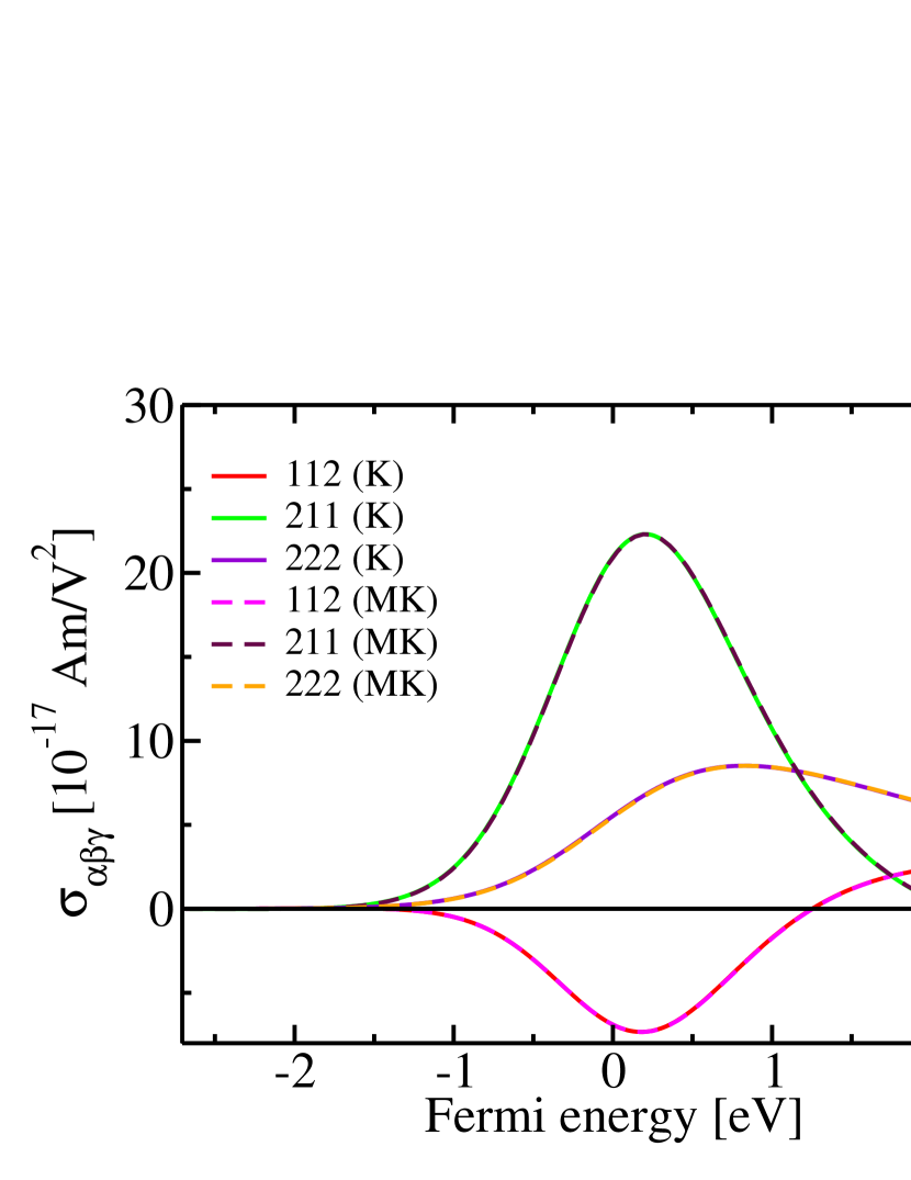
Figure 1: Nonlinear conductivity $\sigma_{\alpha\beta\gamma}$ vs. Fermi energy. Comparison between the Keldysh approach (K) and the Moyal-Keldysh approach (MK). $\alpha^{\rm R}=2$ eVÅ, $\Delta V=1$ eV, $\Gamma=1.36$ eV, and $\hat{{\boldsymbol{M}}}\|-\hat{{\boldsymbol{e}}}_{x}$ are used in the calculation. Both approaches yield identical results.

Fig. 1 shows the comparison between the Keldysh and the Moyal-Keldysh approaches for the parameters $\alpha^{\rm R}=2$ eVÅ, $\Delta V=1$ eV, and $\Gamma=1.36$ eV when the magnetization points in the $-x$ direction. The figure demonstates that the Keldysh and the Moyal-Keldysh approaches yield identical results for the nonlinear conductivity $\sigma_{\alpha\beta\gamma}$, which corroborates the validity of both approaches. In agreement with the symmetry analysis in Sec. II.4 the following tensor components are zero (not shown in the figure): $\sigma_{111}$, $\sigma_{122}$, $\sigma_{212}$, $\sigma_{221}$. Moreover, symmetry dictates that $\sigma_{112}=\sigma_{121}$ (therefore, we show only $\sigma_{112}$ in the figure). When we compare the maxima of the UMR and the NLHE we find that they are comparable in magnitude. When we investigate the dependence of the UMR and of the NLHE on $\Gamma$ and on $\alpha^{\rm R}$ in the figures below we find that this property persists also when these parameters are changed.

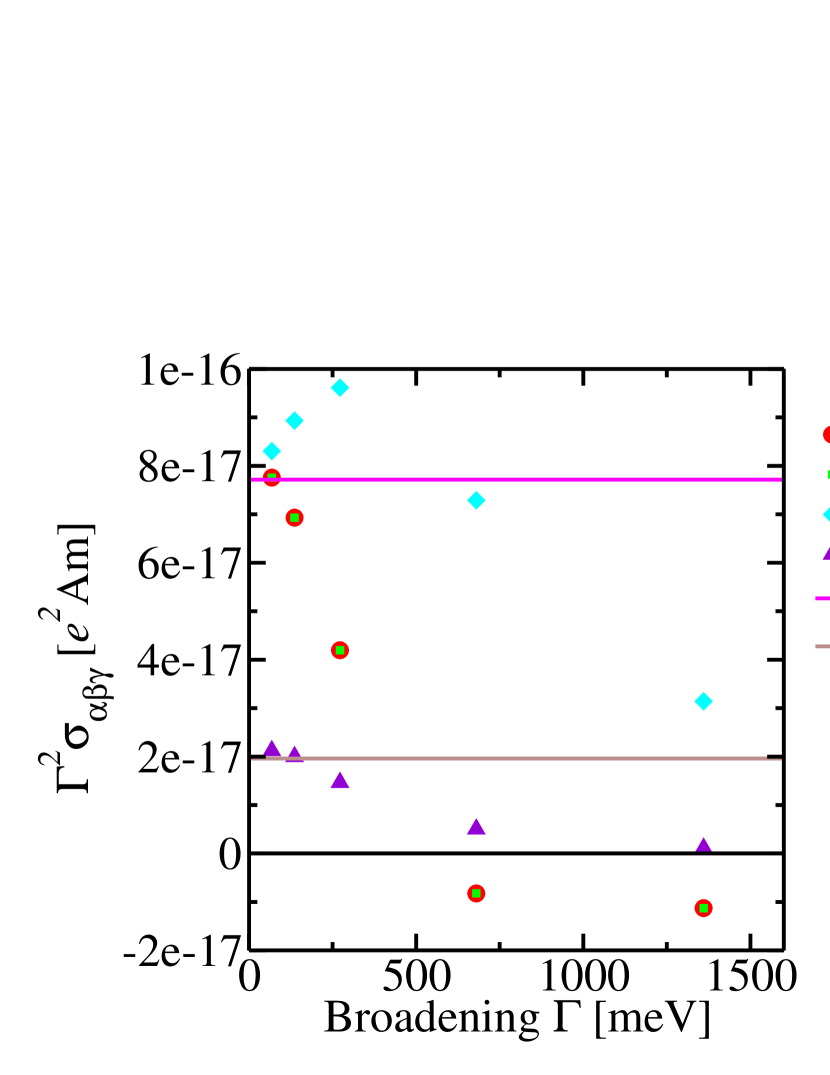
Figure 2: Tensor $\Gamma^{2}\sigma_{\alpha\beta\gamma}$ vs. broadening $\Gamma$ when $\hat{{\boldsymbol{M}}}\|-\hat{{\boldsymbol{e}}}_{x}$, $\alpha^{\rm R}=720$ meVÅ, $\mathcal{E}_{\rm F}=0$, and $\Delta V=1$ eV. Solid lines show the results of the clean-limit Boltzmann (CLB) expression Eq. (33), while the results obtained from Eq. (28) are shown by symbols. CLB is symmetric under any permution of the indices of $\sigma_{\alpha\beta\gamma}$. Consequently, we show only 112 (CLB) in the figure, because 211 (CLB) and 121 (CLB) are equal to it.

In order to study the dependence of the UMR and of the NLHE on the broadening $\Gamma$, we show the $\Gamma$-dependence of the nonlinear conductivity in Fig. 2 at the Fermi energy $\mathcal{E}_{\rm F}=0$, Rashba parameter $\alpha^{\rm R}=720$ meVÅ, and exchange splitting $\Delta V=1$ eV, when $\hat{{\boldsymbol{M}}}$ points in the $-x$ direction. In order to facilitate the illustration of the entire range from small values of $\Gamma$ up to large values of $\Gamma$ we plot $\Gamma^{2}\sigma_{ijk}$ in this figure, because the factor $\Gamma^{2}$ compensates the $\propto\Gamma^{-2}$-behaviour expected in the clean limit according to Eq. (32) and Eq. (39). The clean-limit Boltzmann result Eq. (40) is shown in the figure as well by solid horizontal lines (CLB). The figure shows that the deviations of the clean-limit behaviour from the complete Keldysh results become substantial when $\Gamma$ gets large. Such deviations might contribute to the discrepancies found between the Boltzmann-formalism calculations and the experiment in NiMnSb [12]. Since the Boltzmann formalism yields a tensor $\sigma^{\rm(Boltz)}_{\alpha\beta\gamma}$ that is symmetric [37, 38, 39, 13, 12] under permutation of the indices $\alpha$, $\beta$, and $\gamma$, we show in Fig. 2 only the component $\sigma^{\rm(Boltz)}_{112}$ of the NLHE. In contrast, the Keldysh formalism predicts $\sigma^{\rm(Boltz)}_{112}\neq\sigma^{\rm(Boltz)}_{211}$ when the clean-limit expression does not hold, i.e., when $\Gamma$ is sufficiently large. Clearly, one may argue generally that the violation $\sigma^{\rm(Boltz)}_{112}\neq\sigma^{\rm(Boltz)}_{211}$ indicates that the relaxation time approximation within the Boltzmann formalism fails on the quantitative level. Therefore, when the violation $\sigma^{\rm(Boltz)}_{112}\neq\sigma^{\rm(Boltz)}_{211}$ is established experimentally in a given material, one might consider this as an indication that one needs to go beyond the Boltzmann formalism with constant relaxation time approximation to describe this effect theoretically.

Figure 3: Nonlinear conductivity tensor $\sigma_{\alpha\beta\gamma}$ vs. Fermi energy when $\hat{{\boldsymbol{M}}}\|-\hat{{\boldsymbol{e}}}_{x}$, $\alpha^{\rm R}=720$ meVÅ, $\Delta V=1$ eV, and $\Gamma=68$ meV.

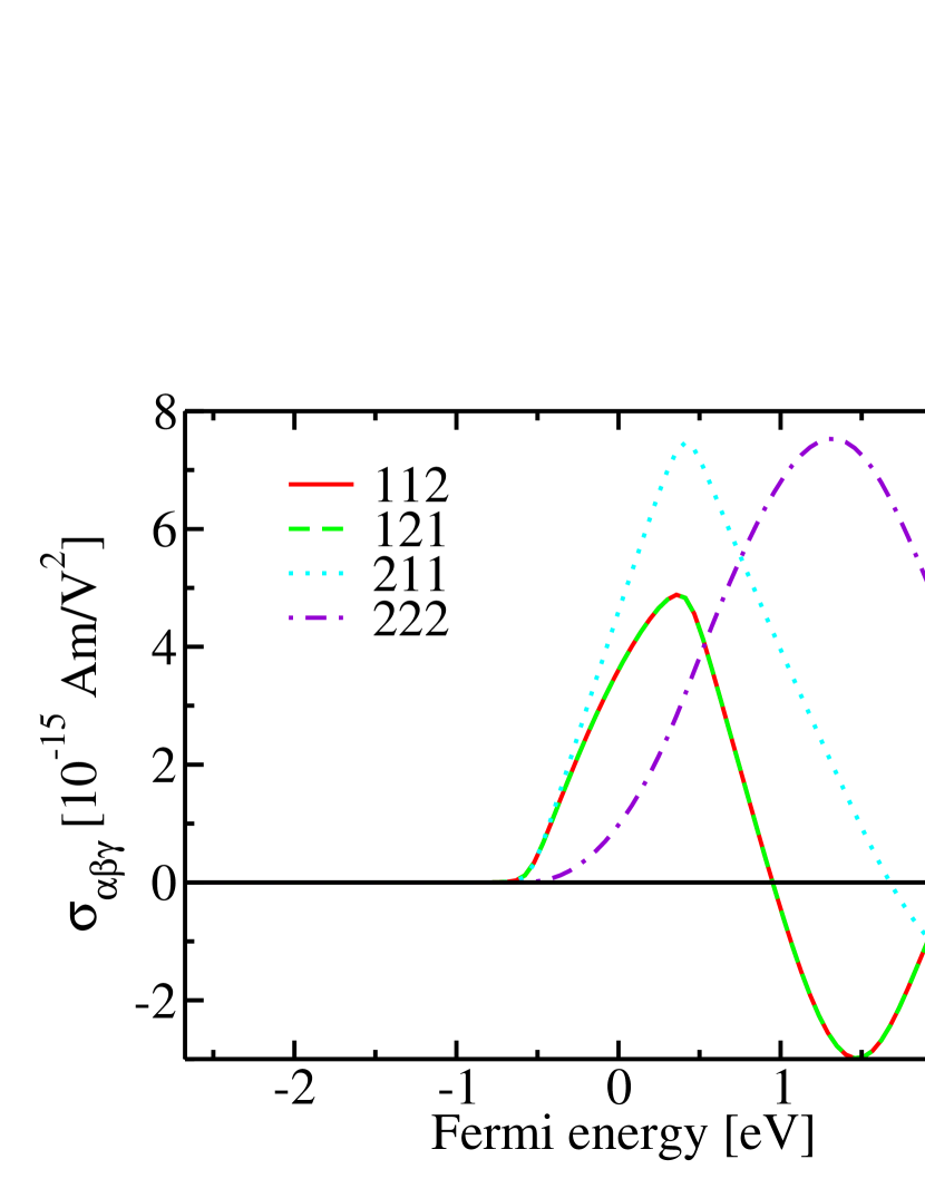
Figure 4: Nonlinear conductivity tensor $\sigma_{\alpha\beta\gamma}$ vs. Fermi energy when $\hat{{\boldsymbol{M}}}\|-\hat{{\boldsymbol{e}}}_{x}$, $\alpha^{\rm R}=720$ meVÅ, $\Delta V=1$ eV, and $\Gamma=136$ meV.

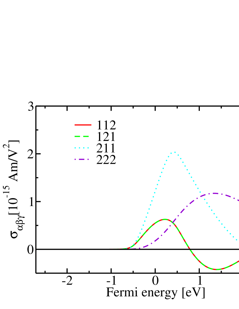
Figure 5: Nonlinear conductivity tensor $\sigma_{\alpha\beta\gamma}$ vs. Fermi energy when $\hat{{\boldsymbol{M}}}\|-\hat{{\boldsymbol{e}}}_{x}$, $\alpha^{\rm R}=720$ meVÅ, $\Delta V=1$ eV, and $\Gamma=272$ meV.

In order to study the dependence of the UMR and of the NLHE on the Fermi energy $\mathcal{E}_{\rm F}$ we show the nonlinear conductivity tensor $\sigma_{\alpha\beta\gamma}$ as a function of Fermi energy when the Rashba parameter is $\alpha^{\rm R}=720$ meVÅ  and when $\hat{{\boldsymbol{M}}}$ points in the $-x$ direction for the broadenings $\Gamma=68$ meV, $\Gamma=136$ meV, $\Gamma=272$ meV, $\Gamma=680$ meV, and $\Gamma=1.36$ eV, in Fig. 3, Fig. 4, Fig. 5, Fig. 6, and Fig. 7, respectively. For these parameters the bandstructure of the Rashba model exhibits a crossing between the first band and the second band at around 1.84 eV, and the band minimum of the first band is at -0.53 eV, while the band minimum of the second band is at 0.47 eV. These band structure properties are visible in Fig. 3: The conductivities vanish below the band minimum of the first band, where the density of states is zero. Around 1.84 eV, where the two bands cross, the conductivities exhibit maxima. The NLHE components exhibit additional maxima around 0.47 eV, where the minimum of the second band is located. These features start to change qualitatively if the broadening $\Gamma$ increases towards the scale of the energy spacing between these features. Since we discussed the $\Gamma$-dependence in Fig. 2 only based on a single Fermi energy $\mathcal{E}_{\rm F}$, we discuss it now a second time by comparing Fig. 3 through Fig. 7 in order to see if qualitative features such as maxima, minima and zeros in the curves are modified by $\Gamma$. As discussed in Fig. 2 we expect that $\sigma_{\alpha\beta\gamma}\propto\tau^{2}\propto\Gamma^{-2}$ when $\Gamma$ is small. Based on this scaling we expect an increase of $\sigma_{\alpha\beta\gamma}$ by a factor of 4 when going from Fig. 4 to Fig. 3. This expectation is roughly satisfied and we attribute the deviations to the size of $\Gamma$, which is not small enough to yield the exact $\propto\Gamma^{-2}$ behaviour of the clean limit. At larger values of $\Gamma$ this $\propto\Gamma^{-2}$ rule becomes less and less predictive. For example the curves in Fig. 5 and Fig. 6 differ substantially qualitatively.

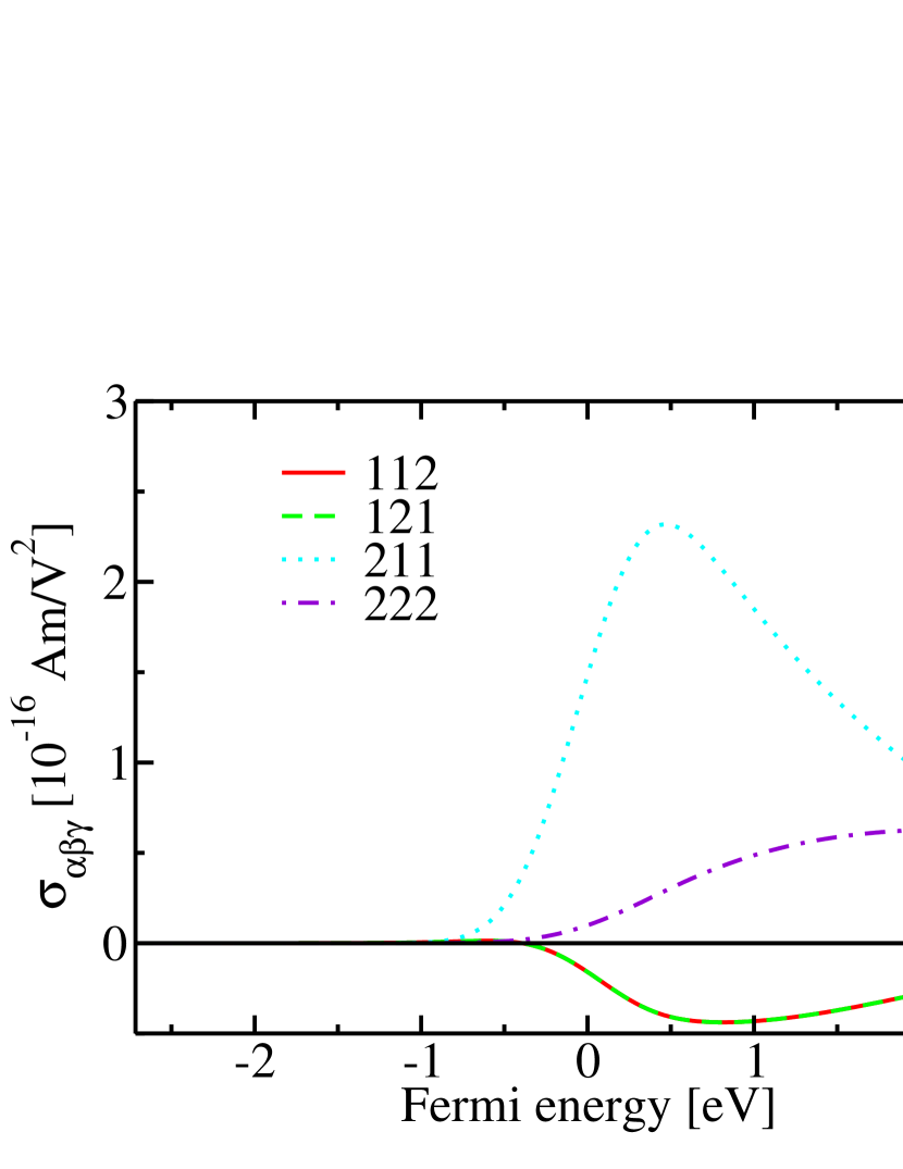
Figure 6: Nonlinear conductivity tensor $\sigma_{\alpha\beta\gamma}$ vs. Fermi energy when $\hat{{\boldsymbol{M}}}\|-\hat{{\boldsymbol{e}}}_{x}$, $\alpha^{\rm R}=720$ meVÅ, $\Delta V=1$ eV, and $\Gamma=680$ meV.

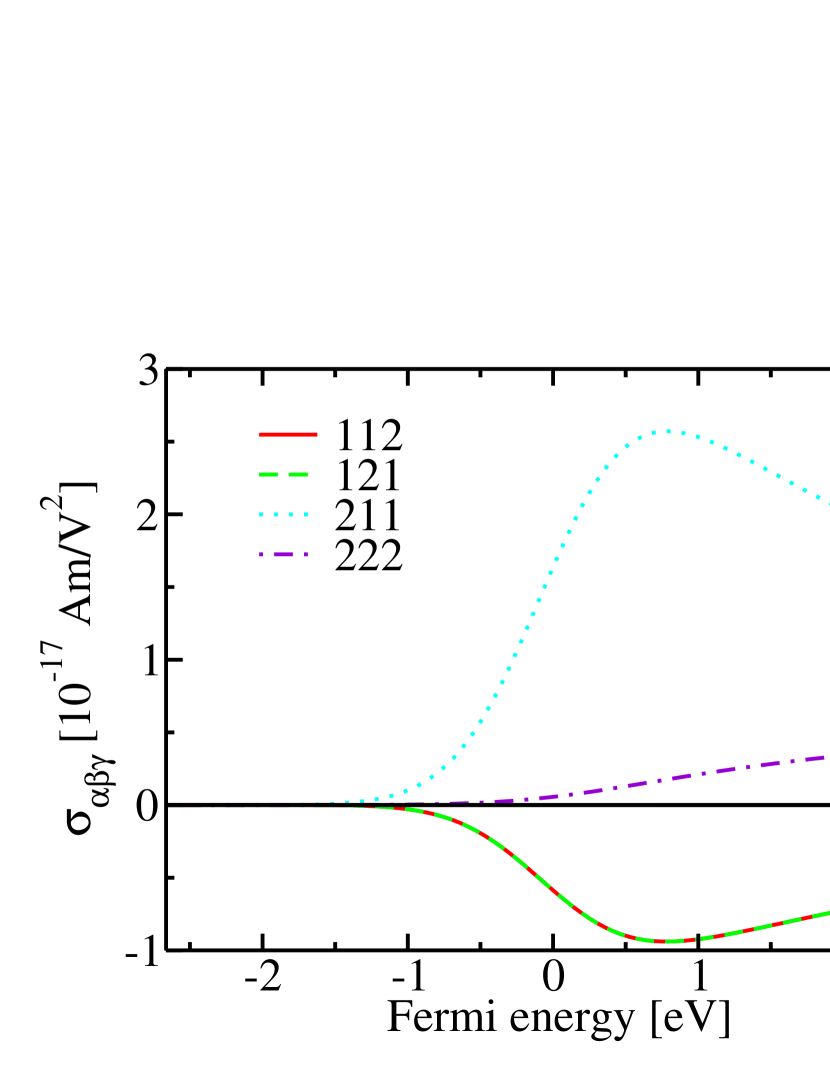
Figure 7: Nonlinear conductivity tensor $\sigma_{\alpha\beta\gamma}$ vs. Fermi energy when $\hat{{\boldsymbol{M}}}\|-\hat{{\boldsymbol{e}}}_{x}$, $\alpha^{\rm R}=720$ meVÅ, $\Delta V=1$ eV, and $\Gamma=1.36$ eV.

Next, we investigate the dependence on the Rashba parameter $\alpha^{\rm R}$. First, we fix the broadening to $\Gamma=136$ meV and vary $\alpha^{\rm R}$. Fig. 8, Fig. 9, Fig. 4, and Fig. 10 show the nonlinear conductivity tensor for $\alpha^{\rm R}=144$ meVÅ, $\alpha^{\rm R}=360$ meVÅ, $\alpha^{\rm R}=720$ meVÅ, and $\alpha^{\rm R}=1439$ meVÅ, respectively. Here, we observe that the maxima of $\sigma_{\alpha\beta\gamma}$ increase stronger than linearly with $\alpha^{\rm R}$. Comparing for example Fig. 4 and Fig. 10 we find that $\sigma_{211}$ and $\sigma_{222}$ increase by roughly one order of magnitude when $\alpha^{\rm R}$ is doubled. In order to investigate this strong $\alpha^{\rm R}$-dependence in more detail we plot the tensor $\sigma_{\alpha\beta\gamma}/(\alpha^{\rm R})^{3}$ in Fig. 11 for the fixed Fermi energy of $\mathcal{E}_{\rm F}=0$. The division of the nonlinear conductivity by the third power of the Rashba parameter facilitates the illustration of the entire range of $\alpha^{\rm R}$ considered here. The component $\sigma_{222}/(\alpha^{\rm R})^{3}$ depends roughly linearly on $\alpha^{\rm R}$ in the range considered in the figure. Consequently, in a coarse approximation $\sigma_{\alpha\beta\gamma}\propto(\alpha^{\rm R})^{4}$ roughly predicts the trend in the range considered in the figure. In contrast, the NLHE depends less strongly on $\alpha^{\rm R}$ at this particular Fermi energy and consequently the components of $\sigma_{\alpha\beta\gamma}/(\alpha^{\rm R})^{3}$ that correspond to the NLHE decrease with increasing $\alpha^{\rm R}$ in the range considered in the figure.

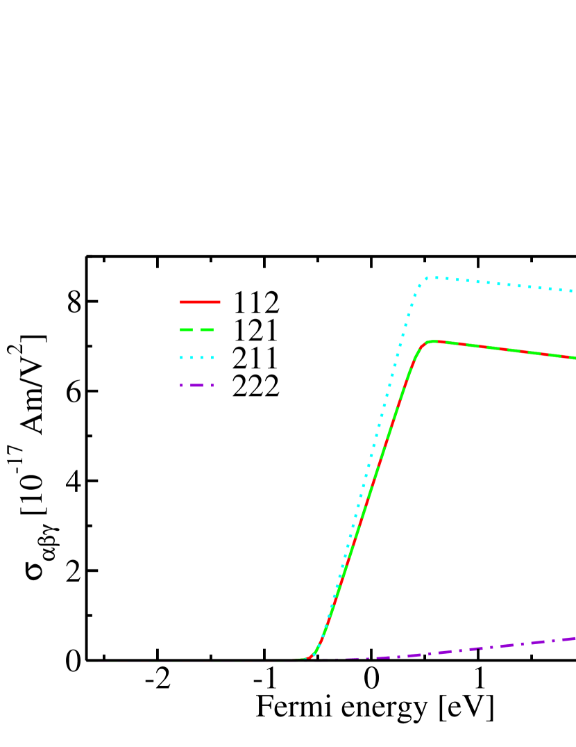
Figure 8: Nonlinear conductivity tensor $\sigma_{\alpha\beta\gamma}$ vs. Fermi energy when $\hat{{\boldsymbol{M}}}\|-\hat{{\boldsymbol{e}}}_{x}$, $\alpha^{\rm R}=144$ meVÅ, $\Delta V=1$ eV, and $\Gamma=136$ meV.

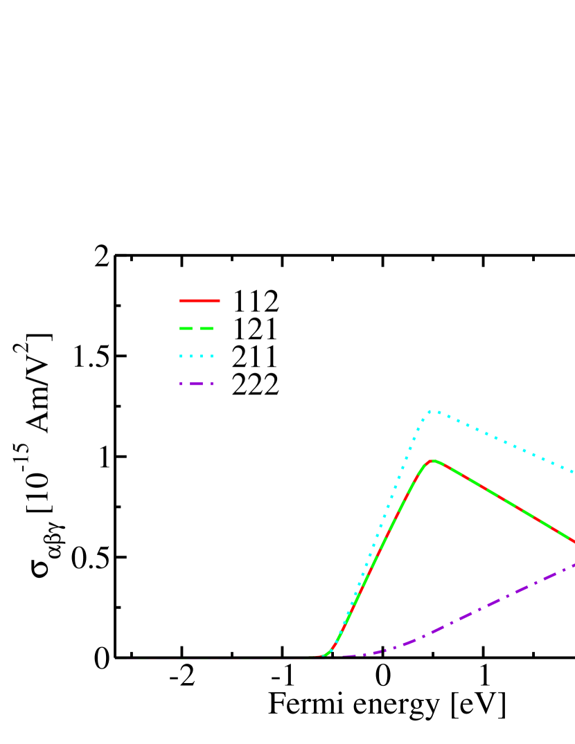
Figure 9: Nonlinear conductivity tensor $\sigma_{\alpha\beta\gamma}$ vs. Fermi energy when $\hat{{\boldsymbol{M}}}\|-\hat{{\boldsymbol{e}}}_{x}$, $\alpha^{\rm R}=360$ meVÅ, $\Delta V=1$ eV, and $\Gamma=136$ meV.

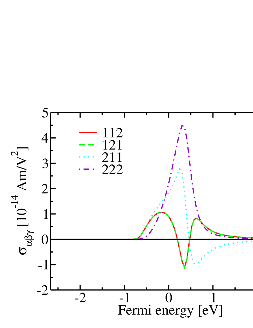
Figure 10: Nonlinear conductivity tensor $\sigma_{\alpha\beta\gamma}$ vs. Fermi energy when $\hat{{\boldsymbol{M}}}\|-\hat{{\boldsymbol{e}}}_{x}$, $\alpha^{\rm R}=1439$ meVÅ, $\Delta V=1$ eV, and $\Gamma=136$ meV.

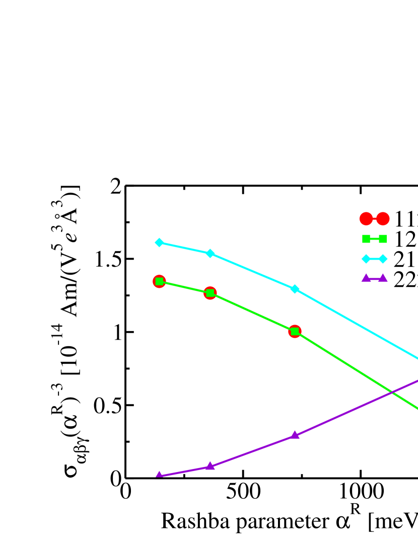
Figure 11: Tensor $\sigma_{\alpha\beta\gamma}/(\alpha^{\rm R})^{3}$ vs. Rashba parameter $\alpha^{\rm R}$ when $\hat{{\boldsymbol{M}}}\|-\hat{{\boldsymbol{e}}}_{x}$, $\Delta V=1$ eV, $\mathcal{E}_{\rm F}=0$ and $\Gamma=136$ meV. Results are shown by symbols and the solid lines only serve as guide to the eye.

Finally, we study the dependence on the Rashba parameter $\alpha^{\rm R}$ at large broadening $\Gamma$ and we set $\Gamma=1.36$ eV. We show the nonlinear conductivities for $\alpha^{\rm R}=360$ meVÅ, $\alpha^{\rm R}=1080$ meVÅ, $\alpha^{\rm R}=1439$ meVÅ, and $\alpha^{\rm R}=2$ eVÅ  in Fig. 12, Fig. 13, Fig. 14, and Fig. 1. When we compare Fig. 14 and Fig. 1 we observe that $\sigma_{\alpha\beta\gamma}$ still increases stronger than linearly with $\alpha^{\rm R}$. However, it does not increase as strongly as for $\Gamma=136$ meV discussed in the preceding paragraph. This behaviour is also illustrated in Fig. 15, which shows the nonlinear conductivity as a function of the Rashba parameter $\alpha^{\rm R}$ when the Fermi energy is set to $\mathcal{E}_{\rm F}=0$.

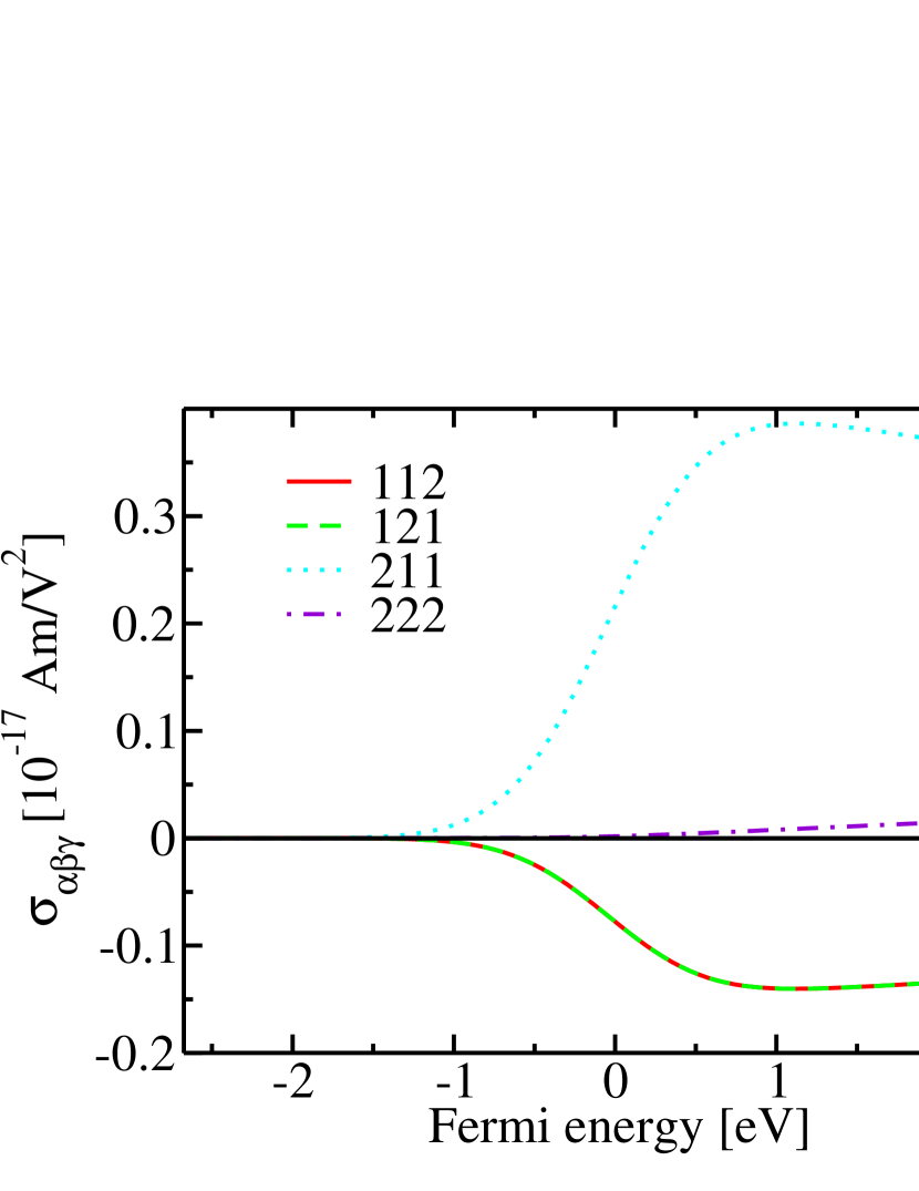
Figure 12: Nonlinear conductivity tensor $\sigma_{\alpha\beta\gamma}$ vs. Fermi energy when $\hat{{\boldsymbol{M}}}\|-\hat{{\boldsymbol{e}}}_{x}$, $\alpha^{\rm R}=360$ meVÅ, $\Delta V=1$ eV, and $\Gamma=1.36$ eV.

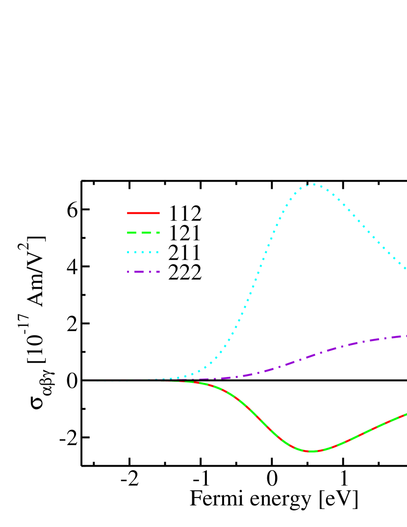
Figure 13: Nonlinear conductivity tensor $\sigma_{\alpha\beta\gamma}$ vs. Fermi energy when $\hat{{\boldsymbol{M}}}\|-\hat{{\boldsymbol{e}}}_{x}$, $\alpha^{\rm R}=1080$ meVÅ, $\Delta V=1$ eV, and $\Gamma=1.36$ eV.

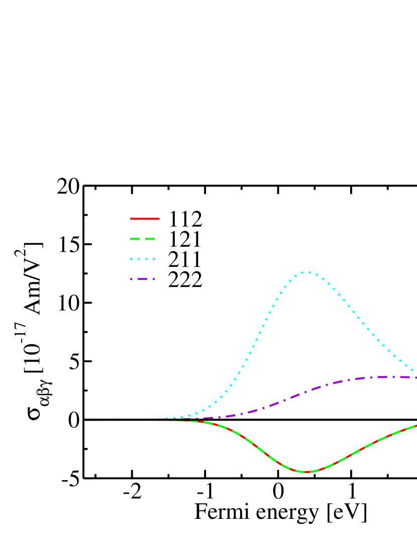
Figure 14: Nonlinear conductivity tensor $\sigma_{\alpha\beta\gamma}$ vs. Fermi energy when $\hat{{\boldsymbol{M}}}\|-\hat{{\boldsymbol{e}}}_{x}$, $\alpha^{\rm R}=1439$ meVÅ, $\Delta V=1$ eV, and $\Gamma=1.36$ eV.

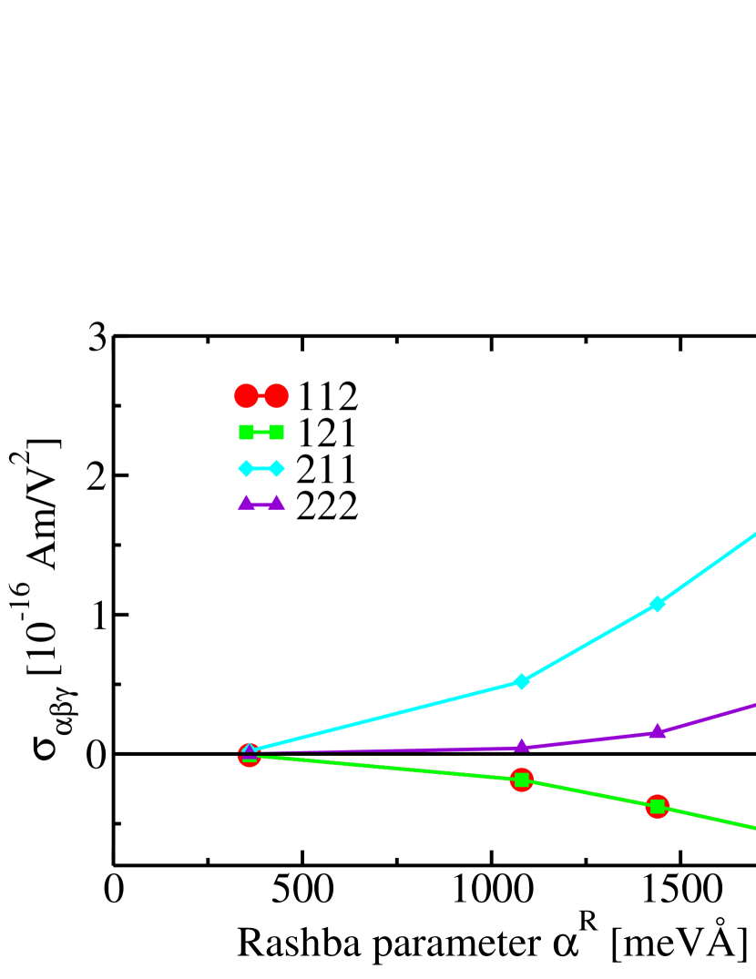
Figure 15: Nonlinear conductivity $\sigma_{\alpha\beta\gamma}$ vs. Rashba parameter $\alpha^{\rm R}$ when $\hat{{\boldsymbol{M}}}\|-\hat{{\boldsymbol{e}}}_{x}$, $\Delta V=1$ eV, $\mathcal{E}_{\rm F}=0$ and $\Gamma=1.36$ eV. Results are shown by symbols and the solid lines only serve as guide to the eye.

It is instructive to compare the magnitude of the UMR and NLHE currents to the magnitude of the photocurrents induced at optical frequencies. According to Ref. [26] laser pulses with 1.55 eV photon energy and intensity 10GW/cm² induce photocurrent densities of the order of magnitude of A/m for Rashba parameters similar to those considered here. The intensity 10GW/cm² corresponds to the electric field strength of the laser field of 2.7 MV/cm. When this field strength induces a photocurrent of 1 A/m, the corresponding second order response coefficient is $\sigma_{\alpha\beta\gamma}=$ A/m (2.7 MV/cm)^-2=$1.37\times 10^{-17}$ Am/V². This is the same order of magnitude as the response coefficients shown in Fig. 12, i.e., at very large broadening of $1.36$ eV. In contrast, we find a response that is larger by three orders of magnitude at small broadening $\Gamma=68$ meV shown in Fig. 3. Since the calculations in Ref. [26] used small broadenings, we may conclude that the nonlinear conductivity at zero frequency is several orders of magnitude larger than the one at optical frequencies when the broadenings are comparable. This finding is consistent with the strong increase and in some cases even divergent behaviour of the quadratic response coefficients as $\omega\rightarrow 0$ found in studies of the inverse Faraday effect [28] and of the photocurrent [27, 40, 41].

IV Summary

We derive the quadratic response of the electric current to an applied electric field using two different formalisms: The usual Keldysh nonequilibrium formalism and the Moyal-Keldysh formalism. The latter approach solves the difficulty of the non-periodic scalar potential associated with a spatially homogeneous time-independent electric field elegantly through the Moyal product. In contrast, the former approach considers a spatially homogeneous time-dependent electric field instead, which may be described by the vector potential, and the zero-frequency limit needs to be taken at the end of the derivation. We show that these two rather different approaches lead to numerically identical results in the ferromagnetic Rashba model, which corroborates their applicability to magnetic Hamiltonians with SOI. Since the Moyal-Keldysh formalism yields the zero-frequency dc response directly, it is presumably the most convenient approach for non-linear response coefficients of high order, because taking the zero-frequency limit in the Keldysh approach becomes more complex as the order of the perturbation increases. When taking the zero-frequency limit in the Keldysh approach we observe that the second order dc conductivity is not identical to the zero-frequency limit of the dc photocurrent expression, because the zero-frequency limit of the 2nd harmonic generation contributes to the second order dc conductivity as well. Additionally, we compare our Keldysh expression in the clean limit analytically to the literature result obtained from the Boltzmann formalism in the constant relaxation time approximation, and find both formulae to agree in this limit. We apply our quadratic response expressions to the ferromagnetic Rashba model in order to study UMR and NLHE. We find the UMR and the NLHE to be of comparable magnitude in this model. Additionally, they scale similarly with the Rashba strength and the quasiparticle broadening. Compared to the response tensor that describes the photocurrent generation at optical frequencies, the zero-frequency effects considered here are several orders of magnitude larger when the parameters in the Rashba parameter are chosen similarly. Our quadratic response expressions are also well-suited to study UMR and NLHE within a first-principles density-functional theory framework.

Appendix A Expressions for the Green functions and the self energies in the Moyal-Keldysh approach

In Eq. (48)

$$G^{<,{\rm II}}_{E_{i},E_{j}}(\mathcal{E})=\left[G^{\rm A}_{E_{i},E_{j}}(\mathcal{E})-G^{\rm R}_{E_{i},E_{j}}(\mathcal{E})\right]$$ (51)

determines the contribution that is proportional to the Fermi function $f(\mathcal{E})$. Here, the retarded function $G^{\rm R}_{E_{i},E_{j}}$ is given by

$$G^{\rm R}_{E_{i},E_{j}}=G^{\rm R}_{0}\Biggl{[}\Sigma^{\rm R}_{E_{i},E_{j}}G^{\rm R}_{0}+\Sigma^{\rm R}_{E_{i}}G^{\rm R}_{E_{j}}+\Sigma^{\rm R}_{E_{j}}G^{\rm R}_{E_{i}}+$$ (52)

$$-\frac{i}{2}\partial_{\pi_{i}}\Sigma^{\rm R}_{E_{j}}\partial_{\pi_{0}}G^{\rm R}_{0}+\frac{i}{2}\partial_{\pi_{i}}(G^{\rm R}_{0})^{-1}\partial_{\pi_{0}}G^{\rm R}_{E_{j}}$$

$$+\frac{i}{2}\partial_{\pi^{0}}\Sigma^{\rm R}_{E_{j}}\partial_{\pi_{i}}G^{\rm R}_{0}-\frac{i}{2}\partial_{\pi^{0}}(G^{\rm R}_{0})^{-1}\partial_{\pi^{i}}G^{\rm R}_{E_{j}}$$

$$-\frac{i}{2}\partial_{\pi_{j}}\Sigma^{\rm R}_{E_{i}}\partial_{\pi_{0}}G^{\rm R}_{0}+\frac{i}{2}\partial_{\pi_{j}}(G^{\rm R}_{0})^{-1}\partial_{\pi_{0}}G^{\rm R}_{E_{i}}$$

$$+\frac{i}{2}\partial_{\pi_{0}}\Sigma^{\rm R}_{E_{i}}\partial_{\pi_{j}}G^{\rm R}_{0}-\frac{i}{2}\partial_{\pi_{0}}(G^{\rm R}_{0})^{-1}\partial_{\pi_{j}}G^{\rm R}_{E_{i}}$$

$$+\frac{1}{4}\partial_{\pi_{i}}\partial_{\pi_{j}}(G^{\rm R}_{0})^{-1}\partial_{\pi_{0}}\partial_{\pi_{0}}G^{\rm R}_{0}$$

$$-\frac{1}{4}\partial_{\pi_{0}}\partial_{\pi_{j}}(G^{\rm R}_{0})^{-1}\partial_{\pi_{0}}\partial_{\pi_{i}}G^{\rm R}_{0}$$

$$-\frac{1}{4}\partial_{\pi_{0}}\partial_{\pi_{i}}(G^{\rm R}_{0})^{-1}\partial_{\pi_{0}}\partial_{\pi_{j}}G^{\rm R}_{0}$$

$$+\frac{1}{4}\partial_{\pi_{0}}\partial_{\pi_{0}}(G^{\rm R}_{0})^{-1}\partial_{\pi_{j}}\partial_{\pi_{i}}G^{\rm R}_{0}\Biggr{]}$$

and $G^{\rm A}_{E_{i},E_{j}}=[G^{\rm R}_{E_{i},E_{j}}]^{\dagger}$, where

$$G^{\rm R}_{E_{i}} =G^{\rm R}_{0}\Biggl{[}\Sigma^{\rm R}_{E_{i}}+\frac{i}{2}\frac{c}{\hbar}\Bigl{[}\frac{\partial}{\partial\mathcal{E}}(G^{\rm R}_{0})^{-1}G^{\rm R}_{0}\frac{\partial}{\partial k_{i}}(G^{\rm R}_{0})^{-1}$$ (53)

$$-\frac{\partial}{\partial k_{i}}(G^{\rm R}_{0})^{-1}G^{\rm R}_{0}\frac{\partial}{\partial\mathcal{E}}(G^{\rm R}_{0})^{-1}\Bigr{]}\Biggr{]}G^{\rm R}_{0}.$$

Additionally,

$$G^{<,{\rm I}}_{E_{i},E_{j}}=G^{\rm R}_{0}\Biggl{[}\Sigma^{<,{\rm I}}_{E_{i},E_{j}}G^{\rm A}_{0}+\Sigma^{<,{\rm I}}_{E_{i}}G^{\rm A}_{E_{j}}+\Sigma^{<,{\rm I}}_{E_{j}}G^{\rm A}_{E_{i}}+$$ (54)

$$-\frac{i}{2}\partial_{\pi_{i}}\Sigma^{\rm R}_{E_{j}}[G^{\rm A}_{0}-G^{\rm R}_{0}]+\frac{i}{2}\partial_{\pi_{i}}(G^{\rm R}_{0})^{-1}\partial_{\pi_{0}}G^{<,{\rm I}}_{E_{j}}$$

$$+\frac{i}{2}\partial_{\pi_{i}}(G^{\rm R}_{0})^{-1}G^{<,{\rm II}}_{E_{j}}$$

$$+\frac{i}{2}\Sigma^{<,{\rm II}}_{E_{j}}\partial_{\pi_{i}}G^{\rm A}_{0}+\frac{i}{2}\partial_{\pi^{0}}\Sigma^{<,{\rm I}}_{E_{j}}\partial_{\pi_{i}}G^{\rm A}_{0}$$

$$-\frac{i}{2}[(G^{\rm A}_{0})^{-1}-(G^{\rm R}_{0})^{-1}]\partial_{\pi^{i}}G^{\rm A}_{E_{j}}-\frac{i}{2}\partial_{\pi^{0}}(G^{\rm R})^{-1}\partial_{\pi^{i}}G^{<,{\rm I}}_{E_{j}}$$

$$-\frac{i}{2}\partial_{\pi_{j}}\Sigma^{\rm R}_{E_{i}}[G^{\rm A}_{0}-G^{\rm R}_{0}]+\frac{i}{2}\partial_{\pi_{j}}(G^{\rm R}_{0})^{-1}\partial_{\pi_{0}}G^{<,{\rm I}}_{E_{i}}$$

$$+\frac{i}{2}\partial_{\pi_{j}}(G^{\rm R}_{0})^{-1}G^{<,{\rm II}}_{E_{i}}$$

$$+\frac{i}{2}\partial_{\pi_{0}}\Sigma^{<,{\rm I}}_{E_{i}}\partial_{\pi_{j}}G^{\rm A}_{0}+\frac{i}{2}\Sigma^{<,{\rm II}}_{E_{i}}\partial_{\pi_{j}}G^{\rm A}_{0}$$

$$-\frac{i}{2}[(G^{\rm A}_{0})^{-1}-(G^{\rm R}_{0})^{-1}]\partial_{\pi_{j}}G^{\rm A}_{E_{i}}-\frac{i}{2}\partial_{\pi_{0}}(G^{\rm R}_{0})^{-1}\partial_{\pi_{j}}G^{<,{\rm I}}_{E_{i}}$$

$$+\frac{1}{2}\partial_{\pi_{i}}\partial_{\pi_{j}}(G^{\rm R}_{0})^{-1}[\partial_{\pi_{0}}G^{\rm A}_{0}-\partial_{\pi_{0}}G^{\rm R}_{0}]$$

$$-\frac{1}{4}\partial_{\pi_{0}}\partial_{\pi_{j}}(G^{\rm R}_{0})^{-1}[\partial_{\pi_{i}}G^{\rm A}_{0}-\partial_{\pi_{i}}G^{\rm R}_{0}]$$

$$-\frac{1}{4}[\partial_{\pi_{j}}(G^{\rm A}_{0})^{-1}-\partial_{\pi_{j}}(G^{\rm R}_{0})^{-1}]\partial_{\pi_{0}}\partial_{\pi_{i}}G^{\rm A}_{0}$$

$$-\frac{1}{4}\partial_{\pi_{0}}\partial_{\pi_{i}}(G^{\rm R}_{0})^{-1}[\partial_{\pi_{j}}G^{\rm A}_{0}-\partial_{\pi_{j}}G^{\rm R}_{0}]$$

$$-\frac{1}{4}[\partial_{\pi_{i}}(G^{\rm A}_{0})^{-1}-\partial_{\pi_{i}}(G^{\rm R}_{0})^{-1}]\partial_{\pi_{0}}\partial_{\pi_{j}}G^{\rm A}_{0}$$

$$+\frac{1}{2}[\partial_{\pi_{0}}(G^{\rm A}_{0})^{-1}-\partial_{\pi_{0}}(G^{\rm R}_{0})^{-1}]\partial_{\pi_{j}}\partial_{\pi_{i}}G^{\rm A}_{0}\Biggr{]}$$

determines the contribution that is proportional to the energy-derivative of the Fermi function $f^{\prime}(\mathcal{E})=\partial f/\partial\mathcal{E}$, and

$$G^{<,{\rm III}}_{E_{i},E_{j}}=G^{\rm R}_{0}\Biggl{[}\Sigma^{<,{\rm III}}_{E_{i},E_{j}}G^{\rm A}_{0}+\frac{i}{2}\partial_{\pi_{i}}(G^{\rm R}_{0})^{-1}G^{<,{\rm I}}_{E_{j}}$$ (55)

$$+\frac{i}{2}\Sigma^{<,{\rm I}}_{E_{j}}\partial_{\pi_{i}}G^{\rm A}_{0}+\frac{i}{2}\partial_{\pi_{j}}(G^{\rm R}_{0})^{-1}G^{<,{\rm I}}_{E_{i}}$$

$$+\frac{i}{2}\Sigma^{<,{\rm I}}_{E_{i}}\partial_{\pi_{j}}G^{\rm A}_{0}+\frac{1}{4}\partial_{\pi_{i}}\partial_{\pi_{j}}(G^{\rm R}_{0})^{-1}[G^{\rm A}_{0}-G^{\rm R}_{0}]$$

$$+\frac{1}{4}[(G^{\rm A}_{0})^{-1}-(G^{\rm R}_{0})^{-1}]\partial_{\pi_{j}}\partial_{\pi_{i}}G^{\rm A}_{0}\Biggr{]}$$

determines the contribution that is proportional to the second energy-derivative of the Fermi function $f^{\prime\prime}(\mathcal{E})=\partial^{2}f/\partial\mathcal{E}^{2}$. Here,

$$G^{<}_{E_{i},I} =G^{\rm R}_{0}\Sigma^{<}_{E_{i},I}G^{\rm A}_{0}$$ (56)

$$-\frac{i}{2}\frac{c}{\hbar}\Biggl{[}G^{\rm R}_{0}\left[\frac{\partial H}{\partial k_{i}}+\frac{\partial\Sigma^{\rm R}_{0}}{\partial k_{i}}\right]\left[G^{\rm A}_{0}-G^{\rm R}_{0}\right]$$

$$-\left[G^{\rm A}_{0}-G^{\rm R}_{0}\right]\left[\frac{\partial H}{\partial k_{i}}+\frac{\partial\Sigma^{A}_{0}}{\partial k_{i}}\right]G^{\rm A}_{0}\Biggr{]}.$$

In the Gaussian disorder approximation we determine the self energies from the equations [30]

$$\Sigma^{\eta,\#}=\mathcal{V}\int\frac{{\rm d}^{D}k}{(2\pi)^{D}}G^{\eta,\#},$$ (57)

$$\Sigma^{\eta,\#}_{E_{i}}=\mathcal{V}\int\frac{{\rm d}^{D}k}{(2\pi)^{D}}G^{\eta,\#}_{E_{i}},$$ (58)

and

$$\Sigma^{\eta,\#}_{E_{i},E_{j}}=\mathcal{V}\int\frac{{\rm d}^{D}k}{(2\pi)^{D}}G^{\eta,\#}_{E_{i},E_{j}},$$ (59)

where $\mathcal{V}$ quantifies the strength of the disorder scattering and $\eta={\rm R,A,}<$. If $\eta\neq<$ we leave $\#$ blank, otherwise $\#={\rm I,II,III}$. Since the Green functions $G^{\eta,\#}$, $G^{\eta,\#}_{E_{i}}$ and $G^{\eta,\#}_{E_{i},E_{j}}$ depend on the self-energies $\Sigma^{\eta,\#}$, $\Sigma^{\eta,\#}_{E_{i}}$, and $\Sigma^{\eta,\#}_{E_{i},E_{j}}$, the equations Eq. (57), Eq. (58) and Eq. (59) need to be solved self-consistently. It is straightforward to extend these expressions into the $T$-matrix approximation [30].

References

- Avci et al. [2015a] C. O. Avci, K. Garello, J. Mendil, A. Ghosh, N. Blasakis, M. Gabureac, M. Trassin, M. Fiebig, and P. Gambardella, Magnetoresistance of heavy and light metal/ferromagnet bilayers, APPLIED PHYSICS LETTERS 107, 192405 (2015a).
- Avci et al. [2015b] C. O. Avci, K. Garello, A. Ghosh, M. Gabureac, S. F. Alvarado, and P. Gambardella, Unidirectional spin Hall magnetoresistance in ferromagnet/normal metal bilayers, Nature physics 11, 570 (2015b).
- Kim et al. [2016] J. Kim, P. Sheng, S. Takahashi, S. Mitani, and M. Hayashi, Spin hall magnetoresistance in metallic bilayers, Phys. Rev. Lett. 116, 097201 (2016).
- Olejník et al. [2015] K. Olejník, V. Novák, J. Wunderlich, and T. Jungwirth, Electrical detection of magnetization reversal without auxiliary magnets, Phys. Rev. B 91, 180402(R) (2015).
- Avci et al. [2017] C. O. Avci, M. Mann, A. J. Tan, P. Gambardella, and G. S. D. Beach, A multi-state memory device based on the unidirectional spin hall magnetoresistance, Applied Physics Letters 110, 203506 (2017).
- Zhang and Vignale [2016] S. S.-L. Zhang and G. Vignale, Theory of unidirectional spin hall magnetoresistance in heavy-metal/ferromagnetic-metal bilayers, Phys. Rev. B 94, 140411(R) (2016).
- Avci et al. [2018] C. O. Avci, J. Mendil, G. S. D. Beach, and P. Gambardella, Origins of the unidirectional spin hall magnetoresistance in metallic bilayers, Phys. Rev. Lett. 121, 087207 (2018).
- Yin et al. [2017] Y. Yin, D.-S. Han, M. C. H. de Jong, R. Lavrijsen, R. A. Duine, H. J. M. Swagten, and B. Koopmans, Thickness dependence of unidirectional spin-hall magnetoresistance in metallic bilayers, Applied Physics Letters 111, 232405 (2017).
- Guillet et al. [2021] T. Guillet, A. Marty, C. Vergnaud, M. Jamet, C. Zucchetti, G. Isella, Q. Barbedienne, H. Jaffrès, N. Reyren, J.-M. George, and A. Fert, Large rashba unidirectional magnetoresistance in the fe/ge(111) interface states, Phys. Rev. B 103, 064411 (2021).
- Lv et al. [2018] Y. Lv, J. Kally, D. Zhang, J. S. Lee, M. Jamali, N. Samarth, and J.-P. Wang, Unidirectional spin-Hall and Rashba-Edelstein magnetoresistance in topological insulator-ferromagnet layer heterostructures, NATURE COMMUNICATIONS 9, 111 (2018).
- Yasuda et al. [2016] K. Yasuda, A. Tsukazaki, R. Yoshimi, K. S. Takahashi, M. Kawasaki, and Y. Tokura, Large unidirectional magnetoresistance in a magnetic topological insulator, Phys. Rev. Lett. 117, 127202 (2016).
- Železný et al. [2021] J. Železný, Z. Fang, K. Olejník, J. Patchett, F. Gerhard, C. Gould, L. W. Molenkamp, C. Gomez-Olivella, J. Zemen, T. Tichý, T. Jungwirth, and C. Ciccarelli, Unidirectional magnetoresistance and spin-orbit torque in (2021), arXiv:2102.12838 [cond-mat.mes-hall] .
- Sodemann and Fu [2015] I. Sodemann and L. Fu, Quantum nonlinear hall effect induced by berry curvature dipole in time-reversal invariant materials, Phys. Rev. Lett. 115, 216806 (2015).
- Yasuda et al. [2017] K. Yasuda, A. Tsukazaki, R. Yoshimi, K. Kondou, K. S. Takahashi, Y. Otani, M. Kawasaki, and Y. Tokura, Current-nonlinear hall effect and spin-orbit torque magnetization switching in a magnetic topological insulator, Phys. Rev. Lett. 119, 137204 (2017).
- Sterk et al. [2019] W. P. Sterk, D. Peerlings, and R. A. Duine, Magnon contribution to unidirectional spin hall magnetoresistance in ferromagnetic-insulator/heavy-metal bilayers, Phys. Rev. B 99, 064438 (2019).
- Watanabe and Yanase [2020] H. Watanabe and Y. Yanase, Nonlinear electric transport in odd-parity magnetic multipole systems: Application to mn-based compounds, Phys. Rev. Research 2, 043081 (2020).
- Sipe and Shkrebtii [2000] J. E. Sipe and A. I. Shkrebtii, Second-order optical response in semiconductors, Phys. Rev. B 61, 5337 (2000).
- Taguchi et al. [2016a] K. Taguchi, D.-H. Xu, A. Yamakage, and K. T. Law, Photovoltaic anomalous hall effect in line-node semimetals, Phys. Rev. B 94, 155206 (2016a).
- Taguchi et al. [2016b] K. Taguchi, T. Imaeda, M. Sato, and Y. Tanaka, Photovoltaic chiral magnetic effect in weyl semimetals, Phys. Rev. B 93, 201202(R) (2016b).
- Ventura et al. [2017] G. B. Ventura, D. J. Passos, J. M. B. Lopes dos Santos, J. M. Viana Parente Lopes, and N. M. R. Peres, Gauge covariances and nonlinear optical responses, Phys. Rev. B 96, 035431 (2017).
- Taghizadeh and Pedersen [2018] A. Taghizadeh and T. G. Pedersen, Gauge invariance of excitonic linear and nonlinear optical response, Phys. Rev. B 97, 205432 (2018).
- Passos et al. [2018] D. J. Passos, G. B. Ventura, J. M. Viana Parente Lopes, J. M. B. Lopes dos Santos, and N. M. R. Peres, Nonlinear optical responses of crystalline systems: Results from a velocity gauge analysis, Phys. Rev. B 97, 235446 (2018).
- Parker et al. [2019] D. E. Parker, T. Morimoto, J. Orenstein, and J. E. Moore, Diagrammatic approach to nonlinear optical response with application to weyl semimetals, Phys. Rev. B 99, 045121 (2019).
- João and Lopes [2019] S. M. João and J. M. V. P. Lopes, Basis-independent spectral methods for non-linear optical response in arbitrary tight-binding models, Journal of Physics: Condensed Matter 32, 125901 (2019).
- Freimuth et al. [2016] F. Freimuth, S. Blügel, and Y. Mokrousov, Laser-induced torques in metallic ferromagnets, Phys. Rev. B 94, 144432 (2016).
- Freimuth et al. [2021] F. Freimuth, S. Blügel, and Y. Mokrousov, Charge and spin photocurrents in the rashba model, Phys. Rev. B 103, 075428 (2021).
- Ahn et al. [2020] J. Ahn, G.-Y. Guo, and N. Nagaosa, Low-frequency divergence and quantum geometry of the bulk photovoltaic effect in topological semimetals, Phys. Rev. X 10, 041041 (2020).
- Berritta et al. [2016] M. Berritta, R. Mondal, K. Carva, and P. M. Oppeneer, Ab initio theory of coherent laser-induced magnetization in metals, Phys. Rev. Lett. 117, 137203 (2016).
- Ogata and Fukuyama [2015] M. Ogata and H. Fukuyama, Orbital magnetism of bloch electrons i. general formula, Journal of the Physical Society of Japan 84, 124708 (2015).
- Onoda et al. [2006] S. Onoda, N. Sugimoto, and N. Nagaosa, Theory of non-equilibirum states driven by constant electromagnetic fields - Non-commutative quantum mechanics in the Keldysh formalism, PROGRESS OF THEORETICAL PHYSICS 116, 61 (2006).
- Freimuth et al. [2013] F. Freimuth, R. Bamler, Y. Mokrousov, and A. Rosch, Phase-space berry phases in chiral magnets: Dzyaloshinskii-moriya interaction and the charge of skyrmions, Phys. Rev. B 88, 214409 (2013).
- Manchon et al. [2015] A. Manchon, H. C. Koo, J. Nitta, S. M. Frolov, and R. A. Duine, New perspectives for Rashba spin–orbit coupling, Nature materials 14, 871 (2015).
- Carbone et al. [2016] C. Carbone, P. Moras, P. M. Sheverdyaeva, D. Pacilé, M. Papagno, L. Ferrari, D. Topwal, E. Vescovo, G. Bihlmayer, F. Freimuth, Y. Mokrousov, and S. Blügel, Asymmetric band gaps in a rashba film system, Phys. Rev. B 93, 125409 (2016).
- Kim et al. [2013] K.-W. Kim, H.-W. Lee, K.-J. Lee, and M. D. Stiles, Chirality from interfacial spin-orbit coupling effects in magnetic bilayers, Phys. Rev. Lett. 111, 216601 (2013).
- Ast et al. [2007] C. R. Ast, J. Henk, A. Ernst, L. Moreschini, M. C. Falub, D. Pacilé, P. Bruno, K. Kern, and M. Grioni, Giant spin splitting through surface alloying, Phys. Rev. Lett. 98, 186807 (2007).
- Ishizaka et al. [2011] K. Ishizaka, M. S. Bahramy, H. Murakawa, M. Sakano, T. Shimojima, T. Sonobe, K. Koizumi, S. Shin, H. Miyahara, A. Kimura, K. Miyamoto, T. Okuda, H. Namatame, M. Taniguchi, R. Arita, N. Nagaosa, K. Kobayashi, Y. Murakami, R. Kumai, Y. Kaneko, Y. Onose, and Y. Tokura, Giant rashba-type spin splitting in bulk , NATURE MATERIALS 10, 521 (2011).
- Zhang et al. [2021] C.-P. Zhang, X.-J. Gao, Y.-M. Xie, H. C. Po, and K. T. Law, Higher-order nonlinear anomalous hall effects induced by berry curvature multipoles (2021), arXiv:2012.15628 [cond-mat.mes-hall] .
- Deyo et al. [2009] E. Deyo, L. E. Golub, E. L. Ivchenko, and B. Spivak, Semiclassical theory of the photogalvanic effect in non-centrosymmetric systems (2009), arXiv:0904.1917 [cond-mat.mes-hall] .
- Tsirkin and Souza [2021] S. S. Tsirkin and I. Souza, On the separation of hall and ohmic nonlinear responses (2021), arXiv:2106.06522 [cond-mat.mtrl-sci] .
- Zhang et al. [2018] Y. Zhang, H. Ishizuka, J. van den Brink, C. Felser, B. Yan, and N. Nagaosa, Photogalvanic effect in weyl semimetals from first principles, Phys. Rev. B 97, 241118(R) (2018).
- Le et al. [2020] C. Le, Y. Zhang, C. Felser, and Y. Sun, Ab initio study of quantized circular photogalvanic effect in chiral multifold semimetals, Phys. Rev. B 102, 121111(R) (2020).