Quality of the Thermodynamic Uncertainty Relation for Fast and Slow Driving

Abstract

The thermodynamic uncertainty relation originally proven for systems driven into a non-equilibrium steady state (NESS) allows one to infer the total entropy production rate by observing any current in the system. This kind of inference scheme is especially useful when the system contains hidden degrees of freedom or hidden discrete states, which are not accessible to the experimentalist. A recent generalization of the thermodynamic uncertainty relation to arbitrary time-dependent driving allows one to infer entropy production not only by measuring current-observables but also by observing state variables. A crucial question then is to understand which observable yields the best estimate for the total entropy production. In this paper we address this question by analyzing the quality of the thermodynamic uncertainty relation for various types of observables for the generic limiting cases of fast driving and slow driving. We show that in both cases observables can be found that yield an estimate of order one for the total entropy production. We further show that the uncertainty relation can even be saturated in the limit of fast driving.
Keywords: thermodynamic uncertainty relation, entropy production, stochastic thermodynamics
Dated:

1 Introduction

Recent progresses in the field of non-equilibrium statistical physics have reshaped our perspective on conventional thermodynamic notions such as work, heat or entropy production. Defining these thermodynamic observables along single fluctuating trajectories is the key step to build up a theoretical formalism nowadays called stochastic thermodynamics [1, 2, 3, 4]. As a key property of these small mesoscopic systems fluctuations and their relation to universal non-equilibrium properties are of special interest from a theoretical as well as from an operational or experimental point of view. A well-established paradigm for such a connection is the fluctuation-dissipation theorem (FDT) relating equilibrium fluctuations to the dissipation rate in driven systems near equilibrium [5]. Milestones in the field of stochastic thermodynamics inter alia deal with similar connections for systems far away from equilibrium: from fluctuation theorems [6, 7, 8, 9, 10, 11, 12, 13, 14, 15] and generalizations of the FDT [16, 17, 18, 19, 20] to the Harada-Sasa relation connecting the violation of the FDT to energy dissipation [21, 22].

A more recent development in this lineup is the so-called thermodynamic uncertainty relation (TUR), which connects the fluctuations or precision of any current in the system to the total entropy production rate [23, 24]. For an overdamped Langevin system or a Markovian system on a discrete set of states driven into a NESS the thermodynamic uncertainty relation for finite observation times $\mathcal{T}$ reads [25, 26]

$$D_{J}(\mathcal{T})\sigma(\mathcal{T})/J(\mathcal{T})^{2}\geq 1$$ (1)

with current $J(\mathcal{T})$, its diffusion coefficient $D_{J}(\mathcal{T})$ quantifying fluctuations and the total entropy production rate $\sigma(\mathcal{T})$. Beyond considering the TUR as a trade-off relation between precision and dissipation leading to bounds on the efficiency of biological processes or molecular machines [27, 28, 29] it has been established as a useful tool for inferring entropy production [30, 31, 32, 33]. Hence, numerous attempts have been made to extend the range of applicability of the TUR including underdamped dynamics [34, 35, 36, 37, 38], ballistic transport between different terminals [39], heat engines [40, 28, 41, 42], periodic driving [43, 44, 45, 46, 47], stochastic field theories [48, 49], generalizations to observables that are even under time-reversal [50, 51, 52], first-passage time problems [53, 54, 55] and quantum systems [56, 57, 58, 39, 59, 60, 61, 62, 63].

In this vast lineup of generalizations and ramifications of the TUR each relation has its own region of validity. A unifying uncertainty relation for arbitrary time-dependent driving including the TUR for finite observation times [25, 26], for relaxation processes [64, 65] and for periodically driven systems [47] has been found recently [66]. This relation reads

$$D_{J}(\mathcal{T},{v})\sigma(\mathcal{T},{v})/J(\mathcal{T},{v})^{2}\geq\left[1+\Delta J(\mathcal{T},{v})/J(\mathcal{T},{v})\right]^{2},$$ (2)

where the speed of driving ${v}$ enters as the second argument and $\Delta J(\mathcal{T},{v})$ describes the change of the current with respect to the observation time $\mathcal{T}$ and the speed of driving ${v}$. A similar inequality involving the total entropy production rate can also be derived for state variables [66]. Since their origin lies in the response of the system with respect to a time re-scaling by using a virtual perturbing force [67], these relations should be clearly distinguished from so-called generalized thermodynamic uncertainty relations that are solely a consequence of the fluctuation theorem [68, 69]. Furthermore, the TUR for time-dependent driving (2) involves operationally accessible observables and hence, preserves the desired property of being a trade-off relation between those. It thus remains a useful tool for inferring entropy production, in principle. However, the question remains, which observables yield the best estimate for entropy production.

In this paper, we analyze the quality of the thermodynamic uncertainty relation (TUR) for time-dependent driving (2) in the limiting cases of fast driving and slow driving for overdamped Langevin systems. We show that in each limiting case at least one optimal class of observable exists that generically yields an estimate of order one for the total entropy production rate. We further show that the time-dependent uncertainty relation in ref. [66] simplifies to the conventional form of the steady-state TUR in refs. [23, 24] in the fast-driving limit. We demonstrate that in this limiting case a current proportional to the total entropy production rate can saturate the TUR. For the slow-driving limit we show that the choice of the optimal observable depends on whether or not a non-conservative force is applied. Moreover, we show that these results hold not only for systems with continuous degrees of freedom, but also for systems with a discrete set of states as we illustrate for a driven three-state model.

2 Setup

2.1 Dynamics

We consider a system with one continuous degree of freedom $x(t)$. The dynamics is given by an overdamped Langevin equation

$$\dot{x}(t)=\mu F(x(t),\lambda_{t})+\zeta(t),$$ (3)

where $\zeta(t)$ is a zero-mean Gaussian white noise satisfying

$$\langle\zeta(t)\rangle =0,$$ (4)

$$\langle\zeta(t)\zeta(t^{\prime})\rangle =2D\delta(t-t^{\prime}).$$ (5)

The system is driven by a time-dependent force

$$F(x,\lambda_{t})\equiv f(\lambda_{t})-\partial_{x}V(x,\lambda_{t}),$$ (6)

which consists of a non-conservative force $f(\lambda_{t})$ and a conservative part $-\partial_{x}V(x,\lambda_{t})$. Both contributions depend on a time-dependent protocol $\lambda_{t}\equiv\lambda({v}t)$. Here, ${v}$ denotes the speed of driving and $D\equiv\mu/\beta$ is the diffusion constant, where $\mu$ is the mobility and $\beta$ is the inverse temperature. Equivalently, we can use a Fokker-Planck equation

$$\partial_{t}p(x,t)=-\partial_{x}(\mu F(x,\lambda_{t})-D\partial_{x})p(x,t)$$ (7)

describing the dynamics for the probability $p(x,t)$ to find the system in state $x$ at time $t$. The system is observed up to time $\mathcal{T}$, where the protocol $\lambda_{t}$ evolves from value $\lambda(0)$ to $\lambda(\tau_{f}\equiv{v}\mathcal{T})$. In the following, we keep the final value $\tau_{f}$ of the protocol fixed, i.e., the observation time $\mathcal{T}=\tau_{f}/{v}$ is coupled to the speed of driving. Equation (7) describes probability conservation and hence, is a continuity equation for the probability current

$$j(x,t)\equiv(\mu F(x,\lambda_{t})-D\partial_{x})p(x,t).$$ (8)

2.2 Observables

The framework of stochastic thermodynamics allows us to define several types of observables for arbitrary time-dependent driven systems [3, 66]. These observables depend on the state $x(t)$ of the system or the velocity $\dot{x}(t)\equiv\partial_{t}x(t)$. The first type of observable we are focusing on is called a state variable $a(x,\lambda_{t})$. This variable can be either observed at a fixed observation time

$$a_{\mathcal{T}}\equiv a(x_{\mathcal{T}},\lambda_{\mathcal{T}})$$ (9)

or it can be time-averaged over a finite-time $\mathcal{T}$

$$A_{\mathcal{T}}\equiv\frac{1}{\mathcal{T}}\int_{0}^{\mathcal{T}}\mathrm{d}t\,a(x_{t},\lambda_{t}),$$ (10)

where $x_{t}\equiv x(t)$. The second kind of observable is a current, which is odd under time reversal. Here, we distinguish between a current depending on the time spent in a certain state

$$J^{b}_{\mathcal{T}}\equiv\frac{1}{\mathcal{T}}\int_{0}^{\mathcal{T}}\mathrm{d}t\,\dot{b}(x_{t},\lambda_{t}),$$ (11)

which depends on the time-derivative of a state variable $\dot{b}(x_{t},\lambda_{t})\equiv(\partial_{t}\lambda_{t})\partial_{\lambda}b(x_{t},\lambda)|_{\lambda=\lambda_{t}}$ and a current depending on the velocity, i.e.,

$$J^{d}_{\mathcal{T}}\equiv\frac{1}{\mathcal{T}}\int_{0}^{\mathcal{T}}\mathrm{d}t\,d(x_{t},\lambda_{t})\circ\dot{x}_{t},$$ (12)

where $d(x_{t},\lambda_{t})$ is a function of the state and $\circ$ denotes the Stratonovich product. A further important observable of interest is the mean total entropy production rate

$$\sigma(\mathcal{T},{v})\equiv\frac{1}{\mathcal{T}}\int_{0}^{\mathcal{T}}\mathrm{d}t\,\int\mathrm{d}x\,\frac{j^{2}(x,t)}{Dp(x,t)},$$ (13)

The fluctuations around the mean value $\langle X_{\mathcal{T}}\rangle$ of any of the above introduced observables $X_{\mathcal{T}}\in\{a_{\mathcal{T}},A_{\mathcal{T}},J^{b,d}_{\mathcal{T}}\}$ are quantified by the diffusion coefficient

$$D_{X}(\mathcal{T},{v})\equiv\mathcal{T}\left(\langle X_{\mathcal{T}}^{2}\rangle-\langle X_{\mathcal{T}}\rangle^{2}\right)/2,$$ (14)

where $\langle\cdot\rangle$ denotes the mean value.

2.3 Quality Factors and the Thermodynamic Uncertainty Relation

The recent generalization of the thermodynamic uncertainty relation to arbitrary time-dependent driving [66] can be applied to all types of observables defined in eqs. (9)–(12). For current-type observables $J_{\mathcal{T}}\in\{J^{d}_{\mathcal{T}},J^{b}_{\mathcal{T}}\}$ the uncertainty relation

$$1\geq\frac{\mathcal{R}_{J}(\mathcal{T},{v})}{D_{J}(\mathcal{T},{v})\sigma(\mathcal{T},{v})}$$ (15)

imposes a bound in terms of the response term

$$\mathcal{R}_{J}(\mathcal{T},{v})\equiv[J(\mathcal{T},{v})+\Delta J(\mathcal{T},{v})]^{2}$$ (16)

with mean value $J(\mathcal{T},{v})\equiv\langle J_{\mathcal{T}}\rangle$ and operator $\Delta\equiv\mathcal{T}\partial_{\mathcal{T}}-{v}\partial_{v}$. The term $\Delta J(\mathcal{T},{v})$ describes the change of the current with respect to a slight change of the observation time $\mathcal{T}$ and the speed of driving ${v}$. For state variables $\mathcal{A}_{\mathcal{T}}\in\{a_{\mathcal{T}},A_{\mathcal{T}}\}$ the uncertainty relation

$$1\geq\frac{\mathcal{R}_{\mathcal{A}}(\mathcal{T},{v})}{D_{\mathcal{A}}(\mathcal{T},{v})\sigma(\mathcal{T},{v})}$$ (17)

involves a modified response term

$$\mathcal{R}_{\mathcal{A}}(\mathcal{T},{v})\equiv[\Delta\mathcal{A}(\mathcal{T},{v})]^{2},$$ (18)

where $\mathcal{A}(\mathcal{T},{v})\equiv\langle\mathcal{A}_{\mathcal{T}}\rangle$ denotes the mean value of a state variable.

For both relations eqs. (15) and (17) we define the quality factors as

$$\mathcal{Q}_{J}\equiv\frac{\mathcal{R}_{J}(\mathcal{T},{v})}{D_{J}(\mathcal{T},{v})\sigma(\mathcal{T},{v})}$$ (19)

and

$$\mathcal{Q}_{\mathcal{A}}\equiv\frac{\mathcal{R}_{\mathcal{A}}(\mathcal{T},{v})}{D_{\mathcal{A}}(\mathcal{T},{v})\sigma(\mathcal{T},{v})},$$ (20)

respectively. Both quality factors are always larger than zero and smaller than one. If a quality factor is zero, no information can be inferred about the entropy production by observing the response and fluctuations of an observable. However, if a quality factor is one, the uncertainty relation is saturated and we can determine the total entropy production exactly.

2.4 Time Scale Separation

The aim of this paper is to analyze the limits of fast driving and slow driving. Hence, it is useful to introduce a time-scale separation between the time scale of the system $t_{\mathrm{sys}}$ and the time scale of the driving ${v}^{-1}$. If the relaxation time scales in the system are approximately of the same order of magnitude, we can choose the basic time scale of the system $t_{\mathrm{sys}}$ as this order of magnitude. However, if the relaxation time scales have different orders of magnitudes, e.g., due to a complex topology like energy barriers in the system, we have to distinguish between the limiting cases of fast driving and slow driving: for the fast-driving limit the basic time scale of the system $t_{\mathrm{sys}}$ has to be chosen as the relaxation time scale describing the fastest relaxation. In contrast, for the limit of slow driving we have to chose $t_{\mathrm{sys}}$ as the time scale that describes the slowest relaxation. Depending on the above discussed cases, the fastest or slowest relaxation time scale in the system is proportional to the inverse of the mobility $\mu$. Hence, the mobility is proportional to the inverse of the time scale $t_{\mathrm{sys}}$ of the system. This circumstance allows us to define a scaled mobility

$$\tilde{\mu}\equiv\mu t_{\mathrm{sys}}.$$ (21)

Plugging eq. (21) into eq. (7) and using the substitution $\tau\equiv{v}t=\tau_{f}t/\mathcal{T}$ leads to the scaled Fokker-Planck equation

$$\partial_{\tau}\tilde{p}(x,\tau)=-\left(\frac{\mathcal{T}}{\tau_{f}t_{\mathrm{sys}}}\right)\partial_{x}(\tilde{\mu}F(x,\lambda_{\tau})-\tilde{D}\partial_{x})\tilde{p}(x,\tau)$$ (22)

with a scaled diffusion constant $\tilde{D}\equiv\tilde{\mu}/\beta$. The density $\tilde{p}(x,\tau)\equiv p(x,\tau/{v})$ depends on the speed of driving ${v}$, i.e.,

$$\tilde{p}(x,\tau)=\tilde{p}(x,\tau;{v}).$$ (23)

We further define the scaled probability current as

$$\tilde{j}(x,\tau;{v})\equiv(\tilde{\mu}F(x,\lambda_{\tau})-\tilde{D}\partial_{x})\tilde{p}(x,\tau;{v}).$$ (24)

For the sake of simplicity, we change the notation $\tilde{p}(x,\tau;{v})\to p(x,\tau;{v})$ and $\tilde{j}(x,\tau;{v})\to j(x,\tau;{v})$ in the following. The scaled Fokker-Planck equation (22) then reads

$$\partial_{\tau}p(x,\tau;{v})=({v}t_{\mathrm{sys}})^{-1}\hat{\mathcal{L}}_{\mathrm{FP}}\left(x,\lambda_{\tau}\right)p(x,\tau;{v}),$$ (25)

with the scaled Fokker-Planck operator

$$\hat{\mathcal{L}}_{\mathrm{FP}}\left(x,\lambda_{\tau}\right)\equiv-\partial_{x}(\tilde{\mu}F(x,\lambda_{\tau})-\tilde{D}\partial_{x}).$$ (26)

The general solution of eq. (25) for a given initial distribution $p(x,0)$ reads

$$p(x,\tau;{v})=\hat{U}\left({x},{\tau},{0}\right)p(x,0),$$ (27)

where

$$\hat{U}\left({x},{\tau_{2}},{\tau_{1}}\right)\equiv\overrightarrow{\exp}\left({\int_{\tau_{1}}^{\tau_{2}}\mathrm{d}\tau\,({v}t_{\mathrm{sys}})^{-1}\hat{\mathcal{L}}_{\mathrm{FP}}\left(x,\lambda_{\tau}\right)}\right)$$ (28)

is the time evolution operator and $\overrightarrow{\exp}\left({\cdot}\right)$ denotes a time-ordered exponential. Via eq. (28) we can define the propagator as

$$p(x_{2},\tau_{2}|x_{1},\tau_{1})\equiv\hat{U}\left({x_{2}},{\tau_{2}},{\tau_{1}}\right)\delta(x_{2}-x_{1}),$$ (29)

where $\tau_{2}\geq\tau_{1}$ and $\delta(\cdot)$ denotes a Dirac delta.

The mean values of the state variables (9) and (10) in terms of the scaled time $\tau={v}t=\tau_{f}t/\mathcal{T}$ are given by

$$a(\mathcal{T},{v})\equiv\int\mathrm{d}x\,a(x,\lambda_{\tau_{f}})p(x,\tau_{f};{v})$$ (30)

and

$$A(\mathcal{T},{v})\equiv\frac{1}{\tau_{f}}\int_{0}^{\tau_{f}}\mathrm{d}\tau\,\int\mathrm{d}x\,a(x,\lambda_{\tau})p(x,\tau;{v}),$$ (31)

respectively, whereas the mean values of the currents (11) and (12) are given by

$$J_{b}(\mathcal{T},{v})\equiv\frac{v}{\tau_{f}}\int_{0}^{\tau_{f}}\mathrm{d}\tau\,\int\mathrm{d}x\,\dot{b}(x,\lambda_{\tau})p(x,\tau;{v})$$ (32)

and

$$J_{d}(\mathcal{T},{v})\equiv\frac{1}{t_{\mathrm{sys}}\tau_{f}}\int_{0}^{\tau_{f}}\mathrm{d}\tau\,\int\mathrm{d}x\,d(x,\lambda_{\tau})j(x,\tau;{v}),$$ (33)

respectively. Here, $\dot{b}(x,\lambda_{\tau})\equiv\partial_{\tau}b(x,\lambda_{\tau})$ is the time-derivative in terms of time scale $\tau$ and

$$j(x,\tau;{v})\equiv(\tilde{\mu}F(x,\lambda_{\tau})-\tilde{D}\partial_{x})p(x,\tau;{v})$$ (34)

is the scaled probability current. Moreover, the mean total entropy production rate (13) in terms of the scaled quantities is given by

$$\sigma(\mathcal{T},{v})\equiv\frac{1}{t_{\mathrm{sys}}\tau_{f}}\int_{0}^{\tau_{f}}\mathrm{d}\tau\,\int\mathrm{d}x\,\frac{j^{2}(x,\tau;{v})}{\tilde{D}p(x,\tau;{v})}.$$ (35)

The diffusion coefficients of the quantities defined in eqs. (9)–(12) can be written in terms of correlation functions between state variables and hence, depend on the propagator (29). Their explicit expressions in terms of the scaled time $\tau$ can be found in A.1.

3 Fast Driving

We first consider the limit of fast driving, where the driving is much faster than the fastest relaxation time scale of the system. The limit of fast driving requires the parameter

$$\epsilon_{f}\equiv\frac{1}{{v}t_{\mathrm{sys}}}\ll 1$$ (36)

to be small, i.e., ${v}^{-1}\ll t_{\mathrm{sys}}$ or equivalently, $\mathcal{T}\ll\tau_{f}t_{\mathrm{sys}}$. This means that the time scale of the driving ${v}^{-1}=\mathcal{T}/\tau_{f}$ is much shorter than the time scale $t_{\mathrm{sys}}$ on which the fastest relaxation of the system takes place. The time evolution operator in eq. (28) can be expanded in terms of $\epsilon_{f}$, i.e.,

$$\hat{U}\left({x},{\tau_{2}},{\tau_{1}}\right)=1+\epsilon_{f}\int_{\tau_{1}}^{\tau_{2}}\mathrm{d}\tau\,\hat{\mathcal{L}}_{\mathrm{FP}}\left(x,\lambda_{\tau}\right)+\mathcal{O}\left(\epsilon_{f}^{2}\right).$$ (37)

Via eq. (27) the density is given by

$$p(x,\tau;{v})=p^{(0)}(x,\tau)+\epsilon_{f}p^{(1)}(x,\tau)+\mathcal{O}\left(\epsilon_{f}^{2}\right)$$ (38)

with zeroth and first order

$$p^{(0)}(x,\tau) =p(x,0),$$ (39)

$$p^{(1)}(x,\tau) =\hat{\mathcal{L}}_{\mathrm{eff}}\left(x,\tau,0\right)p(x,0),$$ (40)

respectively, and

$$\hat{\mathcal{L}}_{\mathrm{eff}}\left(x,\tau,0\right)\equiv\int_{0}^{\tau}\mathrm{d}\tau^{\prime}\,\hat{\mathcal{L}}_{\mathrm{FP}}\left(x,\lambda_{\tau^{\prime}}\right)$$ (41)

being the time-averaged Fokker-Planck operator. The probability current is analogously given by

$$j(x,\tau;{v})=j^{(0)}(x,\tau)+\epsilon_{f}j^{(1)}(x,\tau)+\mathcal{O}\left(\epsilon_{f}^{2}\right)$$ (42)

with zeroth and first order

$$j^{(0)}(x,\tau) =(\tilde{\mu}F(x,\lambda_{\tau})-\tilde{D}\partial_{x})p(x,0),$$ (43)

$$j^{(1)}(x,\tau) =(\tilde{\mu}F(x,\lambda_{\tau})-\tilde{D}\partial_{x})\hat{\mathcal{L}}_{\mathrm{eff}}\left(x,\tau,0\right)p(x,0),$$ (44)

respectively. The leading order of the density (39) shows that the fast driving leaves the initial distribution over the observation time unchanged. The density can then approximately be described by the time-independent initial condition. As a consequence, the leading order of the probability current (43) depends only on the protocol. Furthermore, we can use (37) to get the leading orders of the propagator (29), i.e.,

$$p(x_{2},\tau_{2}|x_{1},\tau_{1})=p^{(0)}(x_{2},\tau_{2}|x_{1},\tau_{1})+\epsilon_{f}p^{(1)}(x_{2},\tau_{2}|x_{1},\tau_{1})+\mathcal{O}\left(\epsilon_{f}^{2}\right).$$ (45)

with zeroth and first order

$$p^{(0)}(x_{2},\tau_{2}|x_{1},\tau_{1}) =\delta(x_{2}-x_{1}),$$ (46)

$$p^{(1)}(x_{2},\tau_{2}|x_{1},\tau_{1}) =\hat{\mathcal{L}}_{\mathrm{eff}}\left(x_{2},\tau_{2},\tau_{1}\right)\delta(x_{2}-x_{1}),$$ (47)

respectively.

To determine the leading orders of the quality factors for the different types of observables, we use eqs. (38), (42) as well as (45) to determine the leading orders of the scaled mean values, eqs. (30)–(33), their response terms, their corresponding diffusion coefficients, eqs. (75)–(A.1), as well as the scaled total entropy production rate (35). Here, all mean values and diffusion coefficients can be written as

$$X(\mathcal{T},{v})\equiv\sum_{n=0}\left(\epsilon_{f}\right)^{n}X^{(n)}(\mathcal{T},{v})$$ (48)

and

$$D_{X}(\mathcal{T},{v})\equiv\sum_{n=0}\left(\epsilon_{f}\right)^{n}D_{X}^{(n)}(\mathcal{T},{v}),$$ (49)

respectively with mean values $X(\mathcal{T},{v})\in\{a(\mathcal{T},{v}),A(\mathcal{T},{v}),\epsilon_{f}J_{b}(\mathcal{T},{v}),J_{d}(\mathcal{T},{v})\}$ and diffusion coefficients $D_{X}(\mathcal{T},{v})\in\{D_{a}(\mathcal{T},{v}),D_{A}(\mathcal{T},{v}),\epsilon_{f}D_{J_{b}}(\mathcal{T},{v}),D_{J_{d}}(\mathcal{T},{v})\}$. Their leading orders and the resulting quality factors are shown in table 1 (see B for details of the derivation).

Table 1: Leading orders of the total entropy production rate, the response terms, the diffusion coefficents and the quality factors of the observables in the limit of fast driving.

Observable $X$	Response Term $\mathcal{R}_{X}$	$D_{X}$	$\sigma(\mathcal{T},{v})$	$\mathcal{Q}_{X}$
$X=a(\mathcal{T},{v})$	$[\Delta a(\mathcal{T},{v})]^{2}=\mathcal{O}\left(\epsilon_{f}^{2}\right)$	$\mathcal{O}\left(\epsilon_{f}\right)$	$\mathcal{O}\left(1\right)$	$\mathcal{O}\left(\epsilon_{f}\right)$
$X=A(\mathcal{T},{v})$	$[\Delta A(\mathcal{T},{v})]^{2}=\mathcal{O}\left(\epsilon_{f}^{2}\right)$	$\mathcal{O}\left(\epsilon_{f}\right)$	$\mathcal{O}\left(1\right)$	$\mathcal{O}\left(\epsilon_{f}\right)$
$X=J_{b}(\mathcal{T},{v})$	$[J_{b}(\mathcal{T},{v})+\Delta J_{b}(\mathcal{T},{v})]^{2}=\mathcal{O}\left(1\right)$	$\mathcal{O}\left(\epsilon_{f}^{-1}\right)$	$\mathcal{O}\left(1\right)$	$\mathcal{O}\left(\epsilon_{f}\right)$
$X=J_{d}(\mathcal{T},{v})$	$[J_{d}(\mathcal{T},{v})+\Delta J_{d}(\mathcal{T},{v})]^{2}=\mathcal{O}\left(1\right)$	$\mathcal{O}\left(1\right)$	$\mathcal{O}\left(1\right)$	$\mathcal{O}\left(1\right)$

The response terms of the state variables vanish like $\epsilon_{f}^{2}$, whereas the response terms of the current observables are of $\mathcal{O}\left(1\right)$. The diffusion coefficients of the state variables vanish like $\epsilon_{f}$ because their variances are of $\mathcal{O}\left(1\right)$. This circumstance is a consequence of the fact that the fast driving conserves the initial distribution. In contrast to the state variables $a(\mathcal{T},{v})$ and $A(\mathcal{T},{v})$ the diffusion coefficient for currents depending on the residence time $D_{J_{b}}$ diverges proportional to $\epsilon_{f}^{-1}$ due to the additional time-derivative of the increment. Together with the fact that the mean total entropy production rate is of $\mathcal{O}\left(1\right)$ these results imply quality factors that vanish linearly with $\epsilon_{f}$ for all observables except for the quality factor $\mathcal{Q}_{J_{d}}$, which is of $\mathcal{O}\left(1\right)$.

To summarize, in the limit of fast driving generically only the current observable $J_{b}(\mathcal{T},{v})$ yields an useful estimate for entropy production. Moreover, the explicit expression for quality factor reads (see B)

$$Q_{J_{d}}\approx\frac{\left[\int_{0}^{\tau_{f}}\mathrm{d}\tau\,\int\mathrm{d}x\,d(x,\lambda_{\tau})j^{(0)}(x,\tau)\right]^{2}}{\left[\int_{0}^{\tau_{f}}\mathrm{d}\tau\,\int\mathrm{d}x\,d^{2}(x,\lambda_{\tau})p(x,0)\right]\left[\int_{0}^{\tau_{f}}\mathrm{d}\tau\,\int\mathrm{d}x\,\left(j^{(0)}(x,\tau)\right)^{2}/(\tilde{D}p(x,0))\right]}.$$ (50)

Here, the response of the current $\Delta J_{d}(\mathcal{T},{v})$ vanishes, which implies that eq. (15) simplifies to the conventional form of the steady-state uncertainty relation in refs. [23, 24]. Furthermore eq. (50) shows that the TUR for time-dependent driving can be saturated for the choice

$$d(x,\lambda_{\tau})=(\tilde{\mu}F(x,\lambda_{\tau})-D[\partial_{x}p(x,0)]/p(x,0))/\tilde{D}=j^{(0)}(x,\tau)/(\tilde{D}p(x,0)),$$ (51)

i.e., when the current is chosen to be the total entropy production rate. We remark that choosing the total entropy production as a current in eq. (15) is in general not allowed due to the fact that the increment for the entropy production $d_{\sigma}\equiv j(x,\tau;{v})/p(x,\tau;{v})$ is not a function of the protocol, i.e., $d_{\sigma}\neq d_{\sigma}(x,\lambda_{\tau})$ (see derivation in ref. [66]). However, in the fast-driving limit the probability current becomes a function of the protocol, i.e., $j(x,\tau;{v})=j^{(0)}(x,\lambda_{\tau})+\mathcal{O}\left(\epsilon_{f}\right)$ and thus the total entropy production rate fulfills the uncertainty relation (15). The fact that the total entropy production can always saturate the TUR in the fast-driving limit is unique for systems with continuous degrees of freedom. For systems with discrete degrees of freedom the definition of the total entropy production rate prevents the saturation of the TUR arbitrary far away from equilibrium. Only for discrete systems close to equilibrium the TUR can be saturated [24, 30]. Moreover, for a constant protocol the result in eq. (50) for fast driving reduces to the result for steady-states in refs. [33, 32] in the limit of short observation times. As a consequence, we have generalized this result to arbitrary time-dependent driving and shown that the total entropy production rate can always saturate the TUR in the short-time limit beyond steady-states for arbitrary driving.

4 Slow Driving

As the second limiting case we consider the limit of slow driving, where the time-dependent driving is much slower than the slowest relaxation time of the system. In this limit the parameter

$$\epsilon_{s}\equiv{v}t_{\mathrm{sys}}\ll 1$$ (52)

is assumed to be small. Here, the time scale of the driving ${v}^{-1}=\mathcal{T}/\tau_{f}$ is large compared to the time scale of the system $t_{\mathrm{sys}}$ describing the slowest relaxation in the system. If the system is initially prepared in an arbitrary distribution $p(x,0)$ it will relax into the stationary state at fixed $\lambda_{0}$. This relaxation process occurs on a time scale that is much faster than the time scale of the external driving. In the following we focus on the slow time scale on which the protocol is changing. Therefore, we assume that the system has already relaxed into the stationary state at $\lambda_{0}$. The density depending only on the slow time scale

$$p(x,\tau;{v})=p^{(0)}(x,\tau)+\epsilon_{s}p^{(1)}(x,\tau)+\mathcal{O}\left(\epsilon_{s}^{2}\right)$$ (53)

relaxes instantaneously into the stationary state

$$p^{(0)}(x,\tau)=p^{s}(x,\lambda_{\tau})$$ (54)

at fixed $\lambda_{\tau}$, i.e., it fulfills

$$\hat{\mathcal{L}}_{\mathrm{FP}}\left(x,\lambda_{\tau}\right)p^{(0)}(x,\tau)=0.$$ (55)

Equation (55) follows by inserting eq. (53) into (25) and by comparing the zeroth orders in $\epsilon_{s}$. The time dependence of the density (54) is given through the protocol $\lambda_{\tau}$. The density corresponds either to a NESS or an equilibrium state at a fixed protocol $\lambda_{\tau}$. If the density is that of a NESS at fixed $\lambda_{\tau}$, the probability current

$$j(x,\tau;{v})=j^{(0)}(x,\tau)+\epsilon_{s}j^{(1)}(x,\tau)+\mathcal{O}\left(\epsilon_{s}^{2}\right)$$ (56)

converges to a finite value

$$j^{(0)}(x,\tau)=(\tilde{\mu}F(x,\lambda_{\tau})-\tilde{D}\partial_{x})p^{s}(x,\lambda_{\tau}).$$ (57)

In contrast if the density is an equilibrium state at fixed $\lambda_{\tau}$, the driving is quasi-static and the probability current vanishes such that $j^{(0)}(x,\tau)=0$ and

$$j(x,\tau;{v})=\epsilon_{s}j^{(1)}(x,\tau)+\mathcal{O}\left(\epsilon_{s}^{2}\right).$$ (58)

The time evolution operator (28) converges to the leading order

$$\hat{U}^{(0)}\left({x},{\tau_{2}},{\tau_{1}}\right)\equiv\lim_{\epsilon_{s}\to 0}\overrightarrow{\exp}\left({\int_{\tau_{1}}^{\tau_{2}}\mathrm{d}\tau\,\epsilon_{s}^{-1}\hat{\mathcal{L}}_{\mathrm{FP}}\left(x,\lambda_{\tau}\right)}\right),$$ (59)

which satisfies

$$\hat{U}^{(0)}\left({x},{\tau_{2}},{\tau_{1}}\right)\rho(x,\tau_{1})=p^{s}(x,\lambda_{\tau_{2}})$$ (60)

for an arbitrary density $\rho(x,\tau)$. Equation (60) shows that the time evolution operator transforms any density into the stationary state at fixed $\lambda_{\tau}$. As a consequence the leading order of the propagator is given by

$$p(x_{2},\tau_{2}|x_{1},\tau_{1})=p(x_{2},\lambda_{\tau_{2}})+\mathcal{O}\left(\epsilon_{s}\right).$$ (61)

We now use eqs. (53), (56) and (61) to determine the leading orders of the scaled mean values, eqs. (30)–(33), their response terms, their corresponding diffusion coefficients, eqs. (75)–(A.1), as well as the scaled total entropy production rate (35). We assume that all mean values and diffusion coefficients can be written as

$$X(\mathcal{T},{v})\equiv\sum_{n=0}\left(\epsilon_{s}\right)^{n}X^{(n)}(\mathcal{T},{v})$$ (62)

and

$$D_{X}(\mathcal{T},{v})\equiv\sum_{n=0}\left(\epsilon_{s}\right)^{n}D_{X}^{(n)}(\mathcal{T},{v})$$ (63)

respectively, with mean values $X(\mathcal{T},{v})\in\{a(\mathcal{T},{v}),A(\mathcal{T},{v}),J_{b,d}(\mathcal{T},{v})\}$ and diffusion coefficients $D_{X}(\mathcal{T},{v})\in\{\epsilon_{s}D_{a}(\mathcal{T},{v}),D_{A}(\mathcal{T},{v}),D_{J_{b,d}}(\mathcal{T},{v})\}$. Their leading orders and the resulting quality factors are shown in table 2 (see C for details of the derivation).

Table 2: Leading orders of the total entropy production rate, the response terms, the diffusion coefficents and the quality factors of the observables in the limit of slow driving. In this limit we have to distinguish whether a non-conservative force $f(\lambda_{t})$ is applied to the system or not: if a non-conservative force is applied the system is in a NESS at fixed $\lambda_{\tau}$ (NESS). However, if only a conservative force is applied, the system is in an equilibrium state for a fixed $\lambda_{\tau}$ (EQ).

Observable $X$	Response Term $\mathcal{R}_{X}$		$D_{X}$	$\sigma(\mathcal{T},{v})$		$\mathcal{Q}_{X}$
	NESS	EQ		NESS	EQ	NESS	EQ
$X=a(\mathcal{T},{v})$	$\mathcal{O}\left(\epsilon_{s}^{2}\right)$	$\mathcal{O}\left(\epsilon_{s}^{2}\right)$	$\mathcal{O}\left(\epsilon_{s}^{-1}\right)$	$\mathcal{O}\left(1\right)$	$\mathcal{O}\left(\epsilon_{s}^{2}\right)$	$\mathcal{O}\left(\epsilon_{s}^{3}\right)$	$\mathcal{O}\left(\epsilon_{s}\right)$
$X=A(\mathcal{T},{v})$	$\mathcal{O}\left(\epsilon_{s}^{2}\right)$	$\mathcal{O}\left(\epsilon_{s}^{2}\right)$	$\mathcal{O}\left(1\right)$	$\mathcal{O}\left(1\right)$	$\mathcal{O}\left(\epsilon_{s}^{2}\right)$	$\mathcal{O}\left(\epsilon_{s}^{2}\right)$	$\mathcal{O}\left(1\right)$
$X=J_{b}(\mathcal{T},{v})$	$\mathcal{O}\left(\epsilon_{s}^{4}\right)$	$\mathcal{O}\left(\epsilon_{s}^{4}\right)$	$\mathcal{O}\left(\epsilon_{s}^{2}\right)$	$\mathcal{O}\left(1\right)$	$\mathcal{O}\left(\epsilon_{s}^{2}\right)$	$\mathcal{O}\left(\epsilon_{s}^{2}\right)$	$\mathcal{O}\left(1\right)$
$X=J_{d}(\mathcal{T},{v})$	$\mathcal{O}\left(1\right)$	$\mathcal{O}\left(\epsilon_{s}^{4}\right)$	$\mathcal{O}\left(1\right)$	$\mathcal{O}\left(1\right)$	$\mathcal{O}\left(\epsilon_{s}^{2}\right)$	$\mathcal{O}\left(1\right)$	$\mathcal{O}\left(\epsilon_{s}^{2}\right)$

The response terms of the state variables vanish like $\epsilon_{s}^{2}$ due to the fact that in the stationary state at fixed $\lambda_{\tau}$ the state variables are invariant under a perturbation that scales the time [67, 70, 66]. The same argument holds for the response term of the current $J_{b}(\mathcal{T},{v})$, which vanishes like $\epsilon_{s}^{4}$. The additional power of two comes from the time-derivative of the increment. If a non-conservative force is applied, the system is driven into a NESS, which implies that the response term of the current $J_{d}(\mathcal{T},{v})$ is of $\mathcal{O}\left(1\right)$ due to the symmetry of the current under the scaling of time in a NESS. However, if only a conservative force is applied, this symmetry does not longer hold because the system is in an equilibrium state at fixed $\lambda_{\tau}$. As a consequence the response term vanishes like $\epsilon_{s}^{2}$. The diffusion coefficient of the state variable $A(\mathcal{T},{v})$ and the current $J_{d}(\mathcal{T},{v})$ are of $\mathcal{O}\left(1\right)$ because their fluctuations are finite in the stationary state at fixed $\lambda_{\tau}$. The instantaneous state variable diverges proportional to $\epsilon_{s}^{-1}$ due to the factor of $\mathcal{T}$ in the definition of its diffusion constant. The diffusion coefficient of the current $J_{b}(\mathcal{T},{v})$ vanishes like $\epsilon_{s}$ due to the time-derivative of its increment. The total entropy production rate is of $\mathcal{O}\left(1\right)$, if a non-conservative force is applied. In this case the probability currents do not vanish and are of $\mathcal{O}\left(1\right)$. In contrast if the system is only driven by a conservative force, the total entropy production rate is of $\mathcal{O}\left(\epsilon_{s}^{2}\right)$. In this case the system is in an equilibrium state at fixed $\lambda_{\tau}$ and hence, the probability currents vanish like $\epsilon_{s}$. Combining these results yields to the leading orders of the quality factors: if a non-conservative force is applied, all quality factors except the quality factor for the current $J_{d}(\mathcal{T},{v})$ vanish. In contrast, if only a conservative force is applied, the quality factors of the state variable $A(\mathcal{T},{v})$ and of the current $J_{b}(\mathcal{T},{v})$ are of $\mathcal{O}\left(1\right)$. The other quality factors vanish asymptotically. To summarize, a useful estimate for the entropy production rate is only possible for the current $J_{d}(\mathcal{T},{v})$, if a non-conservative force is applied or for both, the state variable $A(\mathcal{T},{v})$ and the current $J_{b}(\mathcal{T},{v})$, if the system is driven by a conservative force only.

5 Systems with discrete states: three-state model

Our main results, the scaling of the quality factors in table 1 for fast driving and in table 2 for slow driving, hold generically not only for overdamped Langevin systems but also for systems with a set of discrete states described by a Markovian dynamics as the derivation of the scaling of the quality factors follows the same steps presented in sections 3 and 4. The dynamics for the probability to find the system in a discrete state $i$ is described by the master equation

$$\partial_{t}p_{i}(t;{v})=-\sum_{j}j_{ij}(t;{v})$$ (64)

with probability current

$$j_{ij}(t;{v})\equiv p_{i}(t;{v})k_{ij}(\lambda_{t})-p_{j}(t;{v})k_{ji}(\lambda_{t}),$$ (65)

where we introduced the dependence with respect to the speed parameter ${v}$ as the second argument for both, the probability to find the system in a state $i$ and the probability current between two states $i$ and $j$. The transition rates $k_{ij}(\lambda_{t})$ between two states $i$ and $j$ are time-dependent through the protocol $\lambda_{t}$ and fulfill the local detailed balance condition

$$\frac{k_{ij}(\lambda_{t})}{k_{ji}(\lambda_{t})}=\exp{-\beta\left[E_{j}(\lambda_{t})-E_{i}(\lambda_{t})\right]-\mathcal{A}_{ij}(\lambda_{t})},$$ (66)

where $\beta$ denotes the inverse temperature, $E_{i}(\lambda_{t})$ denotes the time-dependent energy of state $i$ and $\mathcal{A}_{ij}(\lambda_{t})$ is a driving affinity, which drives the system additionally to the time-dependent energies into a non-equilibrium state.

As an example we consider a system with three discrete states, where the energy levels of the states are driven time-dependently through a protocol $\lambda_{t}$. The topology of this network is shown in Fig. 1a).

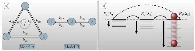
Figure 1: Topology of the two models A and B for the three-state system (a) and schematic of the three-state system with time-dependent energy levels (b). In model A there is a link between states 1 and 3 such that a NESS can be reached by applying a non-conservative force $f$. In model B there is no link betweenstates 1 and 3, which limits the net number of transitions up to a finite observation time $\mathcal{T}$ between two states. The three energy levels have initially the same value $E_{i}(0)=0$ and are decreased over time to a fixed final value $E_{i}(\lambda_{\tau_{f}})=-E^{0}_{i}\tau_{f}^{2}$.

We distinguish between two models: model A contains a link between state 1 and 3. In addition to the time-dependent driving of the energy levels, the system is driven by a constant non-conservative force $f$. In model B there is no link between state 1 and 3. As a consequence the net number of transitions between two states is zero or $\pm 1$, which implies that their fluctuations are not time-extensive. The energy levels of the three states

$$E_{i}(\lambda_{t})\equiv-E^{0}_{i}\lambda_{t},$$ (67)

are driven by a quadratic protocol

$$\lambda_{t}\equiv\left({v}t\right)^{2},$$ (68)

where $E^{0}_{i}$ is the amplitude of the driving and ${v}$ is the speed parameter. The rates are chosen according to the local detailed balance condition (66) and read

$$k_{ij}(\lambda_{t}) \equiv k_{0}^{ij}\exp(-\beta\left[E_{j}(\lambda_{t})-E_{j}(\lambda_{t})\right]/2-f/6),$$ (69)

$$k_{ji}(\lambda_{t}) \equiv k_{0}^{ij}\exp(\beta\left[E_{j}(\lambda_{t})-E_{j}(\lambda_{t})\right]/2+f/6),$$ (70)

where we have chosen the driving affinity as a constant $\mathcal{A}_{ij}(\lambda_{t})=-\mathcal{A}_{ji}(\lambda_{t})=f/3$. The rate amplitudes $k_{0}^{ij}$ determine time scale of the system $t_{\mathrm{sys}}$. In the following, we set all the rate amplitudes to the same value $k_{0}^{ij}\equiv k_{0}=1$ and choose all other parameters $\beta$, $E_{i}(\lambda_{t})$ and $f$ of $\mathcal{O}\left(1\right)$. As a consequence all relaxation times in system are of the same order of magnitude and hence, we are able to choose $t_{\mathrm{sys}}\equiv 1/k_{0}=1$ as outlined in section 2.4. Moreover, we choose the initial distribution $p_{i}(0)$ as the stationary state at fixed $\lambda_{0}$ at the beginning of the driving.

In the following, we analyze the quality factors for both models, A and B in the limits of fast and slow driving for several types of observables. As an example for the instantaneous state variable, we consider the variable

$$a_{\mathcal{T}}^{i}=\delta_{i,i(\mathcal{T})}.$$ (71)

Its mean value is the probability to find the system in state $i$ at the end of the observation time $\mathcal{T}$. Here, $\delta_{i,i(t)}$ is one, if the trajectory $i(t)$ is in state $i$ and zero, otherwise. We further analyze the time-average over this variable

$$A_{\mathcal{T}}^{i}=\frac{1}{\mathcal{T}}\int_{0}^{\mathcal{T}}\mathrm{d}t\,\delta_{i,i(t)},$$ (72)

which is the overall fraction of time the system has spent in state $i$ up to the finite observation time $\mathcal{T}$. For the current-observables we analyze the power

$$P^{i}_{\mathcal{T}}\equiv\frac{1}{\mathcal{T}}\int_{0}^{\mathcal{T}}\mathrm{d}t\,\dot{E}_{i}(\lambda_{t})\delta_{i,i(t)}$$ (73)

exerted at energy level $i$, which is an example for the current $J^{b}_{\mathcal{T}}$ and the rate of directed number of transitions between state $i$ and $j$

$$J^{ij}_{\mathcal{T}}\equiv\frac{1}{\mathcal{T}}\int_{0}^{\mathcal{T}}\mathrm{d}t\,\left[\dot{n}_{ij}(t)-\dot{n}_{ji}(t)\right],$$ (74)

which is an example for the current $J^{d}_{\mathcal{T}}$. Here, $n_{ij}(t)$ denotes the number of transitions between states $i$ and $j$ up to time $t$ along a trajectory $i(t)$. The average value of eq. (74) is the time-averaged probability current between state $i$ and $j$.

In the following we plot inter alia $\mathcal{Q}_{X}/\epsilon_{s,f}^{n}$ against $\epsilon_{s,f}^{-1}$ to analyze the scaling of the quality factor for an observable $X$. Here, $\mathcal{Q}_{X}/\epsilon_{s,f}^{n}$ converges to a constant value for the correct power $n$ (see table 1 and 2) in the limit of fast-driving $\epsilon_{f}^{-1}\to\infty$ and slow-driving $\epsilon_{s}^{-1}\to\infty$, i.e., $\epsilon_{f}\to 0$ and $\epsilon_{s}\to 0$, respectively.

5.1 Model A

The topology of model A in fig. 1a) allows the system to reach a NESS by applying a non-conservative force $f$ or to converge to an equilibrium system by applying only a conservative force. These distinct two cases are especially relevant for the limit of slow driving.

Figure 2 shows the quality factors of the different types of observables defined in eqs. (71)–(74) for a finite non-conservative force $f\geq 0$ (a) and for a vanishing non-conservative force $f=0$ (b).

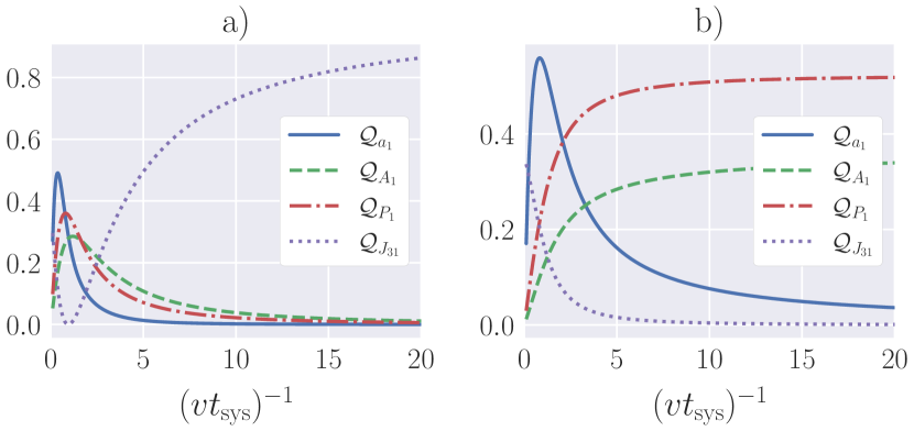
Figure 2: Quality factors of the probability $a_{1}(\mathcal{T},{v})$ to find the system in state 1, of the fraction of time $A_{1}(\mathcal{T},{v})$ the system has spent in state 1, of the power $P_{1}(\mathcal{T},{v})$ applied to state 1 and of the current $J_{31}(\mathcal{T},{v})$ between states 3 and 1. The quality factors are plotted against $({v}t_{\mathrm{sys}})^{-1}$ for $f=1.5$ (a) and for $f=0$ (b). Here, we have set $\beta=1.0$, $E^{0}_{1}=0.5$, $E^{0}_{2}=1.0$ and $E^{0}_{3}=2$.

Comparing the results for fast driving in table 1 and for slow driving in table 2 for the three-state model let us conclude that either the current $J_{31}(\mathcal{T},{v})\equiv\langle J_{\mathcal{T}}^{31}\rangle$ between state 3 and 1 or the time-averaged state variable $A_{1}(\mathcal{T},{v})\equiv\langle A_{\mathcal{T}}^{1}\rangle$ as well as the power $P_{1}(\mathcal{T},{v})\equiv\langle P^{1}_{\mathcal{T}}\rangle$ are the best choice to infer the total entropy production in the respective limiting cases. However, the instantaneous state variable, the probability $a_{1}(\mathcal{T},{v})\equiv\langle a_{\mathcal{T}}^{1}\rangle$ to find the system in state 1, is not an optimal choice for both limiting cases as its quality factor vanishes as shown in fig. 2a) and b). In contrast, we expect that the quality factor for the instantaneous state variable has a maximum and is of $\mathcal{O}\left(1\right)$ for a speed of driving comparable with the time scale of the system, i.e., $({v}t_{\mathrm{sys}})^{-1}\sim 1$. This can be seen for the three-state model in fig. 2a) and b), where the instantaneous state variable yields about $50\%$ of the total entropy production rate.

Next, we analyze the quality factors for the observables defined in eqs. (71)–(74) in the limit of fast-driving. The quality factors for the power, for the fraction of time the system has spent in a certain state, for the probability to find the system in a state and for the time-averaged current between two states are shown in fig. 3a)–d).

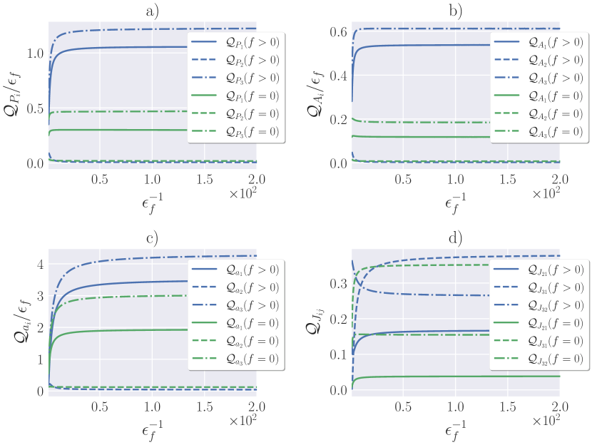
Figure 3: Quality factors in the limit of fast driving for the power (a), for the fraction of time spent in a certain state (b), for the probability to find the system in a certain state (c) and for the time-averaged probability current between two states (d). The quality factors are plotted against the parameter $\epsilon_{f}^{-1}$ and shown for a finite non-conservative force $f=1.5>0$ and for a vanishing force $f=0$. Here, we have set $\beta=1.0$, $E^{0}_{1}=0.5$, $E^{0}_{2}=1.0$ and $E^{0}_{3}=2$.

As predicted by table 1, the quality factors for the state variables $A_{i}(\mathcal{T},{v})$ and $a_{i}(\mathcal{T},{v})$ and the current depending on the residence time $P_{i}(\mathcal{T},{v})$ are proportional to $\epsilon_{f}$ as their quality factors divided by $\epsilon_{f}$ converge to a constant value in the limit $\epsilon_{f}^{-1}\to\infty$ (see fig. 3a)–c)). The quality factor for the current $J_{ij}(\mathcal{T},{v})$ converges to a constant value and is of $\mathcal{O}\left(1\right)$ as shown in fig 3d). The scaling of these quality factors are independent of the force $f$.

In contrast, in the limit of slow driving the scaling of the quality factors depend on the non-conservative force $f$. For $f>0$, the system converges to a NESS at a constant $\lambda_{t}$, whereas for a vanishing force $f=0$ the system converges to an equilibrium state at constant $\lambda_{t}$. We first focus on the case of a non-vanishing force $f>0$. The quality factors for the power, for the fraction of time the system has spent in a certain state, for the probability to find the system in a state and for the time-averaged current between two states are shown in fig. 4a)–d).

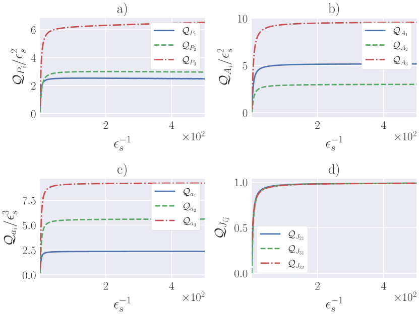
Figure 4: Quality factors in the limit of slow driving for the power (a), for the fraction of time spent in a certain state (b), for the probability to find the system in a certain state (c) and for the time-averaged probability current between two states (d). The quality factors are plotted against the parameter $\epsilon_{s}^{-1}$ and shown for a finite force $f=1.5>0$. Here, we have set $\beta=1.0$, $E^{0}_{1}=0.5$, $E^{0}_{2}=1.0$ and $E^{0}_{3}=2$.

The quality factors for the current $P_{i}(\mathcal{T},{v})$ and the time-averaged state variable $A_{i}(\mathcal{T},{v})$ scale like $\epsilon_{s}^{2}$, whereas it scales for the instantaneous state variable like $\epsilon_{s}^{3}$. In contrast, the only the quality factor of the current $J_{ij}(\mathcal{T},{v})$ yields to a quality factor of $\mathcal{O}\left(1\right)$. There are three quality factors of the time-averaged probability current for each link: $\mathcal{Q}_{J_{21}}$, $\mathcal{Q}_{J_{31}}$ and $\mathcal{Q}_{J_{31}}$. While all three of the quality factors are different in the region of small $\epsilon_{s}^{-1}$, where the slow-driving limit is not yet reached, they converge asymptotically identical to the same value in the limit of slow driving ($\epsilon_{s}^{-1}\to\infty$). This can be understood as follows. When the system is driven slowly enough, it passes different NESSs in the course of time. In each NESS all three currents are identical. As a consequence the quality factors must also be identical. To summarize, the optimal observable leading to a useful estimate for the total entropy production rate is a current $J_{d}(\mathcal{T},{v})$ depending on the velocity or, equivalently, depending on the number of transitions between two discrete states. All other observables yield a quality factor that vanishes at least of order $\epsilon_{s}^{2}$ as predicted in table 2.

Next, we consider the limit of slow driving for a vanishing force $f=0$, where the system is in an equilibrium state at fixed $\lambda_{t}$. The quality factors for the power, for the fraction of time the system has spent in a certain state, for the probability to find the system in a state and for the time-averaged current between two states are shown in fig. 5a)–d).

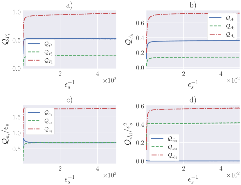
Figure 5: Quality factors in the limit of slow driving for the power (a), for the fraction of time spent in a certain state (b), for the probability to find the system in a certain state (c) and for the time-averaged probability current between two states (d). The quality factors are plotted against the parameter $\epsilon_{s}^{-1}$ and shown for a finite force $f=0$. Here, we have set $\beta=1.0$, $E^{0}_{1}=0.5$, $E^{0}_{2}=1.0$ and $E^{0}_{3}=2$.

In contrast to the case with $f>0$, where the quality factors of the current $P_{i}(\mathcal{T},{v})$ and the state variable $A_{i}(\mathcal{T},{v})$ vanish like $\epsilon_{s}^{2}$ (see fig.4a) and b)), they both converge to a value of $\mathcal{O}\left(1\right)$ as shown in fig. 5a) and b). In the latter case, the time-average state variable $A_{3}(\mathcal{T},{v})$ yields over $60\%$ of the total entropy production rate. The quality factor for the power $P_{3}(\mathcal{T},{v})$ even nearly saturates due to the fact that the total power $P_{\mathrm{tot}}(\mathcal{T},{v})\equiv\sum_{i}P_{i}(\mathcal{T},{v})$ converges to the entropy production rate in the limit of slow driving. The power $P_{3}(\mathcal{T},{v})$ contributes the most to the total power (due to $E^{0}_{3}>E^{0}_{2}>E^{0}_{1}$ as sketched in fig. 1b)) and hence, yields to the best estimate for the total entropy production rate. As shown in fig. 5c) and d) the quality factors for the state variable $a_{i}(\mathcal{T},{v})$ and the for the current $J_{ij}(\mathcal{T},{v})$ vanish like $\epsilon_{s}$ and $\epsilon_{s}^{2}$, respectively. This is an important contrast to the case $f>0$, where the quality factor for the current $J_{ij}(\mathcal{T},{v})$ is of $\mathcal{O}\left(1\right)$.

5.2 Model B

Model B cannot be driven into a NESS due to its topology depicted in fig. 1a). Hence, the system can only reach an equilibrium state, which leads to the generic scaling for the quality factors in the limit of slow driving as shown in table 2 (second columns). However, in this system the topology of the network leads to deviations of the predicted scaling behavior of these quality factors, which are shown in fig. 6a)–d).

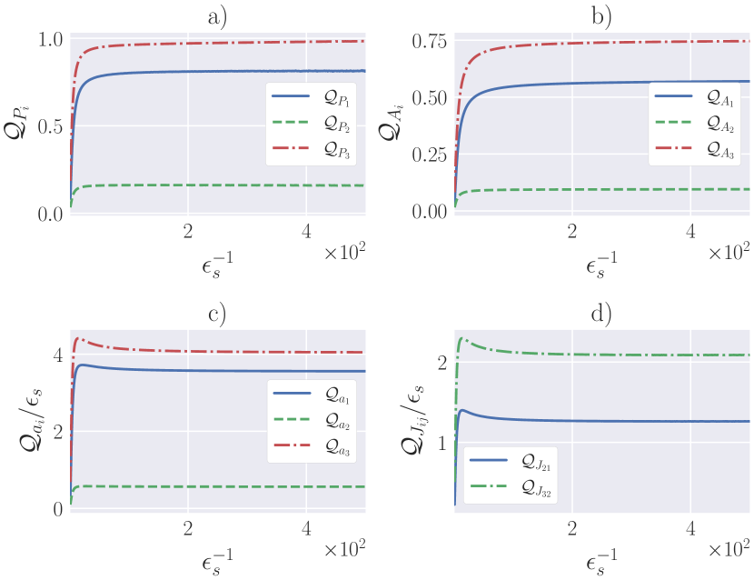
Figure 6: Quality factors in the limit of slow driving for the power (a), for the fraction of time spent in a certain state (b), for the probability to find the system in a certain state (c) and for the time-averaged probability current between two states (d). The quality factors are plotted against the parameter $\epsilon_{s}^{-1}$. Here, we have set $\beta=1.0$, $E^{0}_{1}=0.5$, $E^{0}_{2}=1.0$ and $E^{0}_{3}=2$.

Only the state variable $A_{i}(\mathcal{T},{v})$ and the current $P_{i}(\mathcal{T},{v})$ yield an estimate for the entropy production of $\mathcal{O}\left(1\right)$ as shown in fig. 6a) and b). The quality factors for the instantaneous variable $a_{i}(\mathcal{T},{v})$ and for the current $J_{ij}(\mathcal{T},{v})$ vanish. However, the quality factor of the current $J_{ij}(\mathcal{T},{v})$ does not vanish like $\epsilon_{s}^{2}$ as generically predicted in table 2 but scales like $\epsilon_{s}$. This circumstance follows from the fact that the net number of transitions between two states and consequently also their fluctuations cannot become arbitrary large. As a consequence, the diffusion coefficient of the current is not of $\mathcal{O}\left(1\right)$ but vanishes proportional to $\epsilon_{s}$. This leads to the modified scaling of $\mathcal{O}\left(\epsilon_{s}\right)$ as shown in fig 6d).

6 Conclusion

In this paper, we have analyzed the quality of the thermodynamic uncertainty relation for the limiting cases of fast driving and slow driving. In the limit of fast driving, the generic optimal observable is the current-observable depending on the velocity. The quality factors of all other observables vanish asymptotically. We have further shown that in the limit of fast driving a current proportional to the total entropy production rate can saturate the uncertainty relation. In the limit of slow driving, one has to distinguish whether a driving affinity is additionally applied to the system or not in order to choose the optimal observable. If the system is driven by a driving affinity the optimal observable is the current depending on the velocity. However, if there is no driving affinity only the current depending on the residence time or the time-averaged state variable yields an useful estimate for the total entropy production rate. All other quality factors vanish generically with a power law in the ratio of the relevant time scales. The quality factor of the instantaneous state variable vanishes in both limiting cases. However, as we have illustrated for a three-level system it still can yield a useful estimate when the speed of driving is comparable with the relaxation time scales in the system. Last but not least, an analysis of the quality factors in the three-state model shows that depending on the topology of the system deviations of the generic scaling of the quality factors can occur.

With these results we have introduced first steps for optimizing inference schemes using the thermodynamic uncertainty relation for time-dependent driving. We have focused on the scaling behavior of various classes of observables. In a next step, one could investigate which observable is optimal within each class. Moreover, it would be possible to use a superposition of two observables or to involve correlations between them in order to optimize the bounds on entropy production [71]. Lastly, a further open question is how the quality of the TUR behaves as a function of system size in more complex models.

Appendix A Diffusion Coefficients and Correlation Functions

A.1 Diffusion Coefficients

In this section, we give the explicit expressions for the diffusion coefficients of the observables defined in eqs. (9)–(12). The diffusion coefficients of the state variables (9) and (10) in terms of the scaled time $\tau$ are given by

$$D_{a}(\mathcal{T},{v})=\mathcal{T}\left(\int\mathrm{d}x\,a^{2}(x,\lambda_{\tau_{f}})p(x,\tau_{f};{v})-a(\mathcal{T},{v})^{2}\right)/2$$ (75)

and

$$D_{A}(\mathcal{T},{v})= \frac{\mathcal{T}}{\tau_{f}^{2}}\int_{0}^{\tau_{f}}\mathrm{d}\tau\,\int_{0}^{\tau}\mathrm{d}\tau^{\prime}\,\int\mathrm{d}x\,\int\mathrm{d}x^{\prime}\,a(x,\lambda_{\tau})p(x,\tau|x^{\prime},\tau^{\prime})a(x^{\prime},\lambda_{\tau})p(x^{\prime},\tau;{v})$$

$$-\mathcal{T}/2A(\mathcal{T},{v})^{2},$$ (76)

respectively. Analogously, the diffusion coefficient of the the current (11) is given by

$$D_{J^{b}}(\mathcal{T},{v})= \frac{{v}}{\tau_{f}}\int_{0}^{\tau_{f}}\mathrm{d}\tau\,\int_{0}^{\tau}\mathrm{d}\tau^{\prime}\,\int\mathrm{d}x\,\int\mathrm{d}x^{\prime}\,\dot{b}(x,\lambda_{\tau})p(x,\tau|x^{\prime},\tau^{\prime})\dot{b}(x^{\prime},\lambda_{\tau})p(x^{\prime},\tau;{v})$$

$$-\mathcal{T}/2J_{b}(\mathcal{T},{v})^{2}.$$ (77)

In order to write the diffusion coefficient of the current in eq. (12) in terms of correlation functions between state functions, we use the relation (A.2) in A.2. Plugging eq. (A.2) into the diffusion coefficient (14) of the current depending on the velocity and changing to the time scale $\tau$ yields

$$D_{J^{d}}(\mathcal{T},{v})= \frac{1}{t_{\mathrm{sys}}\tau_{f}}\int_{0}^{\tau_{f}}\mathrm{d}\tau\,\int\mathrm{d}x\,\tilde{D}d^{2}(x,\lambda_{\tau})p(x,\tau;{v})$$

$$+\frac{({v}t_{\mathrm{sys}})^{-1}}{t_{\mathrm{sys}}\tau_{f}}\int_{0}^{\tau_{f}}\mathrm{d}\tau\,\int_{0}^{\tau}\mathrm{d}\tau^{\prime}\,\int\mathrm{d}x\,\int\mathrm{d}x^{\prime}\,\tilde{J}(x,\tau)p(x,\tau|x^{\prime},\tau^{\prime})$$

$$\hskip 85.35826pt\times\{\tilde{J}(x^{\prime},\tau^{\prime})p(x^{\prime},\tau^{\prime};{v})-2\tilde{D}\left[d(x^{\prime},\lambda_{\tau^{\prime}})p(x^{\prime},\tau^{\prime};{v})\right]^{\prime}\}$$

$$-\frac{\mathcal{T}}{2}J_{d}(\mathcal{T},{v})^{2}$$ (78)

with

$$\tilde{J}(x,\tau)\equiv d(x,\lambda_{\tau})j(x,\tau;{v})/p(x,\tau;{v})+\tilde{D}\{d(x,\lambda_{\tau})p(x,\tau;{v})\}^{\prime}/p(x,\tau;{v}).$$ (79)

A.2 Correlation Functions

Throughout this section, we use the original notation for the Fokker-Planck equation introduced in eq. (7) and not the time-scaled notation introduced in section 2.4. In the following, we derive the relation

$$\langle d(x_{t},\lambda_{t})\circ\dot{x}_{t}d(x_{t^{\prime}},\lambda_{t^{\prime}})\circ\dot{x}_{t^{\prime}}\rangle =\,2D\langle d^{2}(x_{t},\lambda_{t})\rangle\delta(t-t^{\prime})$$

$$+\theta(t-t^{\prime})\langle J(x_{t^{\prime}},t^{\prime})\left[J(x_{t},t)-2D\{d(x_{t},\lambda_{t})p(x_{t},t;{v})\}^{\prime}/p(x_{t},t)\right]\rangle$$

$$+\theta(t^{\prime}-t)\langle J(x_{t},t)\left[J(x_{t^{\prime}},t^{\prime})-2D\{d(x_{t},\lambda_{t})p(x_{t},t;{v})\}^{\prime}/p(x_{t^{\prime}},t^{\prime})\right]\rangle$$ (80)

with

$$J(x_{t},t)\equiv d(x_{t},\lambda_{t})j(x_{t},t)/p(x_{t},t)+D\{d(x_{t},\lambda_{t})p(x_{t},t)\}^{\prime}/p(x_{t},t),$$ (81)

where

$$\{d(x_{t},\lambda_{t})p(x_{t},t)\}^{\prime}\equiv\partial_{x}d(x,\lambda_{t})p(x,t)|_{x=x_{t}}.$$ (82)

We introduce the shorthand notation $C_{t}\equiv C(x_{t},\lambda_{t})$ for an arbitrary state function $C(x_{t},\lambda_{t})$. First, we use the Langevin eq. (3) to rewrite the expression

$$\langle d_{t}\circ\dot{x}_{t}d_{t^{\prime}}\circ\dot{x}_{t^{\prime}}\rangle=\langle d_{t}\circ\zeta_{t}d_{t^{\prime}}\circ\zeta_{t^{\prime}}\rangle-\langle d_{t}\mu F_{t}d_{t^{\prime}}\mu F_{t^{\prime}}\rangle+\langle d_{t}\mu F_{t}d_{t^{\prime}}\circ\dot{x}_{t^{\prime}}\rangle+\langle d_{t^{\prime}}\mu F_{t^{\prime}}d_{t}\circ\dot{x}_{t}\rangle$$ (83)

in terms of the noise. Then, we use Itô’s lemma [72] to write the first term in eq. (83) in terms of non-anticipating functions and the noise, i.e.,

$$\langle d_{t}\circ\zeta_{t}d_{t^{\prime}}\circ\zeta_{t^{\prime}}\rangle=\langle d_{t}\cdot\zeta_{t}d_{t^{\prime}}\cdot\zeta_{t^{\prime}}\rangle-D^{2}\langle d^{\prime}_{t}d^{\prime}_{t^{\prime}}\rangle+\langle Dd^{\prime}_{t}d_{t^{\prime}}\circ\left[\dot{x}_{t^{\prime}}-\mu F_{t^{\prime}}\right]\rangle+\langle Dd^{\prime}_{t^{\prime}}d_{t}\circ\left[\dot{x}_{t}-\mu F_{t}\right]\rangle,$$ (84)

where $\cdot$ denotes the Itô product and

$$d^{\prime}_{t}\equiv\partial_{x}d(x,\lambda_{t})|_{x=x_{t}}.$$ (85)

Next, we use Itô’s Isometry [72] to evaluate the first term in eq. (84), which reads

$$\langle d_{t}\cdot\zeta_{t}d_{t^{\prime}}\cdot\zeta_{t^{\prime}}\rangle=2D\delta(t-t^{\prime})\langle d^{2}_{t}\rangle.$$ (86)

Using eqs. (84) and (86) we can rewrite eq. (83) as

$$\langle d_{t}\circ\dot{x}_{t}d_{t^{\prime}}\circ\dot{x}_{t^{\prime}}\rangle= 2D\delta(t-t^{\prime})\langle d^{2}_{t}\rangle-\langle\left[d_{t}\mu F_{t}+Dd^{\prime}_{t}\right]\left[d_{t^{\prime}}\mu F_{t^{\prime}}+Dd^{\prime}_{t^{\prime}}\right]\rangle$$ (87)

$$+\langle\left[d_{t^{\prime}}\mu F_{t^{\prime}}+Dd^{\prime}_{t^{\prime}}\right]d_{t}\circ\dot{x}_{t}\rangle+\langle\left[d_{t}\mu F_{t}+Dd^{\prime}_{t}\right]d_{t^{\prime}}\circ\dot{x}_{t^{\prime}}\rangle.$$

Now, we rewrite the last two terms of eq. (87) in terms of correlation functions between state functions. To do so, we define a variable $B(x,\lambda_{t})$ such that $\partial_{x}B(x,\lambda_{t})=d(x,\lambda_{t})$ and hence, $d(x_{t},\lambda_{t})\circ\dot{x}_{t}=\dot{B}(x_{t},\lambda_{t})-\dot{\lambda}\partial_{\lambda}B(x,\lambda)|_{\lambda=\lambda_{t}}$, where $\dot{B}(x_{t},\lambda_{t})\equiv(\mathrm{d}/\mathrm{d}t)B(x_{t},\lambda_{t})$ is the total time-derivative of the state function $B(x,\lambda_{t})$. The last term in eq. (87) can be written as

$$\langle\left[d_{t}\mu F_{t}+Dd^{\prime}_{t}\right]d_{t^{\prime}}\circ\dot{x}_{t^{\prime}}\rangle=\langle A_{t}\circ\left[\dot{B}_{t^{\prime}}-\dot{\lambda}\partial_{\lambda}B(x_{t^{\prime}},\lambda)|_{\lambda=\lambda_{t^{\prime}}}\right]\rangle,$$ (88)

with $A_{t}\equiv d_{t}\mu F_{t}+Dd^{\prime}_{t}$. Next, we can rewrite the first term on the r.h.s of eq. (88) by applying the derivative after averaging because average values and time derivatives commute in the Stratonovich convention [73], i.e.,

$$\langle A_{t}\dot{B}_{t^{\prime}}\rangle=(\mathrm{d}/\mathrm{d}t^{\prime})\langle A_{t}B_{t^{\prime}}\rangle=(\mathrm{d}/\mathrm{d}t^{\prime})\int\mathrm{d}x\,A(x,\lambda_{t})U\left({x},{t},{t^{\prime}}\right)B(x,\lambda_{t^{\prime}})$$ (89)

for $t>t^{\prime}$ and

$$\langle A_{t}\dot{B}_{t^{\prime}}\rangle=(\mathrm{d}/\mathrm{d}t^{\prime})\int\mathrm{d}x\,B(x,\lambda_{t^{\prime}})U\left({x},{t^{\prime}},{t}\right)A(x,\lambda_{t})$$ (90)

for $t^{\prime}>t$ with time evolution operator

$$U\left({x},{t^{\prime}},{t}\right)\equiv\overrightarrow{\exp}\left({\int_{t}^{t^{\prime}}\mathrm{d}t^{\prime\prime}\,\mathcal{L}_{\mathrm{FP}}\left(x,\lambda_{t^{\prime\prime}}\right)}\right)$$ (91)

and Fokker-Planck operator

$$\mathcal{L}_{\mathrm{FP}}\left(x,\lambda_{\tau}\right)\equiv-\partial_{x}\left(\mu F-D\partial_{x}\right).$$ (92)

Using $(\mathrm{d}/\mathrm{d}t^{\prime})U\left({x},{t^{\prime}},{t}\right)=\mathcal{L}_{\mathrm{FP}}\left(x,t^{\prime}\right)U\left({x},{t^{\prime}},{t}\right)$ and $(\mathrm{d}/\mathrm{d}t^{\prime})U\left({x},{t},{t^{\prime}}\right)=U\left({x},{t},{t^{\prime}}\right)\mathcal{L}_{\mathrm{FP}}\left(x,t^{\prime}\right)$ for eqs. (89) and (90) yields the following expression

$$\langle A_{t}\dot{B}_{t^{\prime}}\rangle =\theta(t-t^{\prime})\langle A_{t}\left[2\nu_{t^{\prime}}d_{t^{\prime}}-\mu F_{t^{\prime}}-Dd^{\prime}_{t^{\prime}}+\dot{\lambda}\partial_{\lambda}B(x_{t^{\prime}},\lambda)|_{\lambda=\lambda_{t^{\prime}}}\right]\rangle$$ (93)

$$+\theta(t^{\prime}-t)\langle A_{t}\left[\mu F_{t^{\prime}}d_{t^{\prime}}+Dd^{\prime}_{t^{\prime}}+\dot{\lambda}\partial_{\lambda}B(x_{t^{\prime}},\lambda)|_{\lambda=\lambda_{t^{\prime}}}\right]\rangle,$$

where $\theta(\cdot)$ is the Heaviside function and $\nu_{t}\equiv j(x_{t},\lambda_{t})/p(x_{t},\lambda_{t})$ is the mean local velocity. Finally, inserting eq. (93) into eq. (87) leads to

$$\langle d_{t}\circ\dot{x}_{t}d_{t^{\prime}}\circ\dot{x}_{t^{\prime}}\rangle =2D\delta(t-t^{\prime})\langle d^{2}_{t}\rangle$$ (94)

$$+\theta(t-t^{\prime})\langle\left[\mu F_{t}d_{t}+Dd^{\prime}_{t}\right]\left[2\nu_{t^{\prime}}d_{t^{\prime}}-\mu F_{t^{\prime}}d_{t^{\prime}}-Dd^{\prime}_{t^{\prime}}\right]\rangle$$

$$+\theta(t^{\prime}-t)\langle\left[\mu F_{t^{\prime}}d_{t^{\prime}}+Dd^{\prime}_{t^{\prime}}\right]\left[2\nu_{t}d_{t}-\mu F_{t}d_{t}-Dd^{\prime}_{t}\right]\rangle,$$

which is identical to eq. (A.2) when identifying the terms $J(x_{t},\lambda_{t})=\mu F_{t^{\prime}}d_{t^{\prime}}+Dd^{\prime}_{t^{\prime}}$ and $J(x_{t},\lambda_{t})-2D{d(x_{t},\lambda_{t})p(x_{t},\lambda_{t})}^{\prime}/p(x_{t},t)=2\nu_{t}d_{t}-\mu F_{t}d_{t}-Dd^{\prime}_{t}$.

Appendix B Limit of Fast Driving

In this section, we derive the scaling properties of the quality factors in the limit of fast driving shown in table 1.

First, we determine the leading order of the total entropy production rate by inserting eqs. (38) and (42) into eq. (35), which yields

$$\sigma(\mathcal{T},{v})=\frac{1}{t_{\mathrm{sys}}}\sigma^{(0)}(\mathcal{T},{v})+\mathcal{O}\left(\epsilon_{f}/t_{\mathrm{sys}}\right)\equiv\frac{1}{t_{\mathrm{sys}}\tau_{f}}\int_{0}^{\tau_{f}}\mathrm{d}\tau\,\int\mathrm{d}x\,\frac{j^{(0)}(x,\tau)^{2}}{\tilde{D}p(x,0)}+\mathcal{O}\left(\epsilon_{f}/t_{\mathrm{sys}}\right).$$ (95)

Obviously, the entropy production rate is of $\mathcal{O}\left(1\right)$ in the limit of fast driving.

Next, we determine the leading orders of the mean values and their response terms. Inserting eqs. (38), (39), (40) into (30) leads to an expression for the instantaneous state variable

$$a(\mathcal{T},{v})=a^{(0)}(\mathcal{T},{v})+\epsilon_{f}a^{(1)}(\mathcal{T},{v})+\mathcal{O}\left(\epsilon_{f}^{2}\right)$$ (96)

with

$$a^{(0)}(\mathcal{T},{v})\equiv\int\mathrm{d}x\,a(x,\lambda_{\tau_{f}})p(x,0)$$ (97)

and

$$a^{(1)}(\mathcal{T},{v})\equiv\int\mathrm{d}x\,a(x,\lambda_{\tau_{f}})\hat{\mathcal{L}}_{\mathrm{eff}}\left(x,\tau_{f},0\right)p(x,0).$$ (98)

The response term of $a(\mathcal{T},{v})$ is consequently given by

$$\mathcal{R}_{a}(\mathcal{T},{v})\equiv\left[\Delta a(\mathcal{T},{v})\right]^{2}=\left[a^{(1)}(\mathcal{T},{v})\right]^{2}\epsilon_{f}^{2}+\mathcal{O}\left(\epsilon_{f}^{3}\right)$$ (99)

due to the fact that $\Delta f(\tau_{f}={v}\mathcal{T})=0$ for an arbitrary function depending only on $\tau_{f}$ and not depending separately on ${v}$ and $\mathcal{T}$. For time-averaged state variables (31) one gets a similar behavior by following the analogous steps above, which leads to the response term

$$\mathcal{R}_{A}(\mathcal{T},{v})\equiv\left[\Delta A(\mathcal{T},{v})\right]^{2}=\left[A^{(1)}(\mathcal{T},{v})\right]^{2}\epsilon_{f}^{2}+\mathcal{O}\left(\epsilon_{f}^{3}\right)$$ (100)

with

$$A^{(1)}(\mathcal{T},{v})\equiv\frac{1}{\tau_{f}}\int_{0}^{\tau_{f}}\int\mathrm{d}x\,a(x,\lambda_{\tau})\hat{\mathcal{L}}_{\mathrm{eff}}\left(x,\tau,0\right)p(x,0).$$ (101)

Furthermore, for the current defined in eq. (32) one finds the following expression for the current

$$J_{b}(\mathcal{T},{v})=\frac{1}{\epsilon_{f}t_{\mathrm{sys}}}\left(J^{(0)}_{b}(\mathcal{T},{v})+\epsilon_{f}J^{(1)}_{b}(\mathcal{T},{v})+\mathcal{O}\left(\epsilon_{f}^{2}\right)\right)$$ (102)

with zeroth order

$$J^{(0)}_{b}(\mathcal{T},{v})\equiv\frac{1}{\tau_{f}}\int_{0}^{\tau_{f}}\int\mathrm{d}x\,\dot{b}(x,\lambda_{\tau})p(x,0)$$ (103)

and first order

$$J^{(1)}_{b}(\mathcal{T},{v})\equiv\frac{1}{\tau_{f}}\int_{0}^{\tau_{f}}\int\mathrm{d}x\,\dot{b}(x,\lambda_{\tau})\hat{\mathcal{L}}_{\mathrm{eff}}\left(x,\tau,0\right)p(x,0).$$ (104)

Using these expressions leads to the response term

$$\mathcal{R}_{J_{b}}(\mathcal{T},{v})\equiv\left[J_{b}(\mathcal{T},{v})+\Delta J_{b}(\mathcal{T},{v})\right]^{2}=\left[J^{(1)}_{b}(\mathcal{T},{v})\right]^{2}(1/t_{\mathrm{sys}}^{2})+\mathcal{O}\left(\epsilon_{f}\right).$$ (105)

Moreover, for the current depending on the velocity we insert eqs. (42), (43) into eq. (34), which leads to

$$J_{d}(\mathcal{T},{v})=\frac{1}{t_{\mathrm{sys}}}J^{(0)}_{d}(\mathcal{T},{v})+\mathcal{O}\left(\epsilon_{f}/t_{\mathrm{sys}}\right)$$ (106)

with zeroth leading order

$$J^{(0)}_{d}(\mathcal{T},{v})\equiv\frac{1}{\tau_{f}}\int_{0}^{\tau_{f}}\mathrm{d}\tau\,\int\mathrm{d}x\,d(x,\lambda_{\tau})j^{(0)}(x,\tau).$$ (107)

The response term consequently reads

$$\mathcal{R}_{J_{d}}(\mathcal{T},{v})\equiv\left[J_{d}(\mathcal{T},{v})+\Delta J_{d}(\mathcal{T},{v})\right]^{2}=\left[J^{(0)}_{d}(\mathcal{T},{v})\right]^{2}\frac{1}{t_{\mathrm{sys}}^{2}}+\mathcal{O}\left(\epsilon_{f}/t_{\mathrm{sys}}^{2}\right).$$ (108)

Now we derive the leading order of the diffusion coefficients. First, using the leading order of the density in (39) and plugging it into eq. (75) yields

$$D_{a}(\mathcal{T},{v})=t_{\mathrm{sys}}\tau_{f}\epsilon_{f}D^{(1)}_{a}(\mathcal{T},{v})+\mathcal{O}\left(\epsilon_{f}^{2}\right)$$ (109)

with

$$D^{(1)}_{a}(\mathcal{T},{v})\equiv\frac{1}{2}\left(\int\mathrm{d}x\,a(x,\lambda_{\tau_{f}})^{2}p(x,0)-\left[\int\mathrm{d}x\,a(x,\lambda_{\tau_{f}})p(x,0)\right]^{2}\right)$$ (110)

for the instantaneous state variable. For all other diffusion coefficients it is sufficient to use the zeroth order of the propagator defined in eq. (46). Plugging this leading order into the diffusion coefficient (A.1) for time-averaged state variable leads to

$$D_{A}(\mathcal{T},{v})=t_{\mathrm{sys}}\tau_{f}\epsilon_{f}D^{(1)}_{A}(\mathcal{T},{v})+\mathcal{O}\left(\epsilon_{f}^{2}\right)$$ (111)

with

$$D^{(1)}_{A}(\mathcal{T},{v})\equiv\frac{1}{\tau_{f}^{2}}\int_{0}^{\tau_{f}}\mathrm{d}\tau\,\int_{0}^{\tau}\mathrm{d}\tau^{\prime}\,\int\mathrm{d}x\,a(x,\lambda_{\tau})a(x,\lambda_{\tau^{\prime}})p(x,0)-\frac{1}{2}A^{(0)}(\mathcal{T},{v})^{2},$$ (112)

where

$$A^{(0)}(\mathcal{T},{v})\equiv\frac{1}{\tau_{f}}\int_{0}^{\tau_{f}}\mathrm{d}\tau\,\int\mathrm{d}x\,a(x,\lambda_{\tau})p(x,0)$$ (113)

is the leading zeroth order of the time-averaged state variable. Furthermore, plugging eq. (46) into (32) yields the diffusion coefficient

$$D_{J_{b}}=\frac{\tau_{f}}{t_{\mathrm{sys}}\epsilon_{f}}\left(D^{(0)}_{J_{b}}(\mathcal{T},{v})+\mathcal{O}\left(\epsilon_{f}\right)\right)$$ (114)

of the current $J_{b}(\mathcal{T},{v})$ with

$$D^{(0)}_{J_{b}}(\mathcal{T},{v})\equiv\frac{1}{\tau_{f}^{2}}\int_{0}^{\tau_{f}}\mathrm{d}\tau\,\int_{0}^{\tau}\mathrm{d}\tau^{\prime}\,\int\mathrm{d}x\,\dot{b}(x,\lambda_{\tau})\dot{b}(x,\lambda_{\tau^{\prime}})p(x,0)-\frac{1}{2}J^{(0)}_{b}(\mathcal{T},{v})^{2},$$ (115)

where $J^{(0)}_{b}(\mathcal{T},{v})$ is defined in eq. (103). For diffusion coefficient of the current depending on the velocity, we insert eq. (46) into (A.1), which leads to

$$D_{J_{d}}(\mathcal{T},{v})=\frac{1}{t_{\mathrm{sys}}}D^{(0)}_{J_{d}}(\mathcal{T},{v})+\mathcal{O}\left(\epsilon_{f}/t_{\mathrm{sys}}\right)$$ (116)

with leading order

$$D^{(0)}_{J_{d}}(\mathcal{T},{v})\equiv\frac{1}{\tau_{f}}\int_{0}^{\tau_{f}}\mathrm{d}\tau\,\int\mathrm{d}x\,d^{2}(x,\lambda_{\tau})p(x,0).$$ (117)

Finally, we use the above derived results to determine the leading orders of all quality factors. First, by using eqs. (95),  (99) and (109) we can determine the quality factor

$$Q_{a}\equiv\frac{\mathcal{R}_{a}(\mathcal{T},{v})}{\sigma(\mathcal{T},{v})D_{a}(\mathcal{T},{v})}\approx\frac{\left[a^{(1)}(\mathcal{T},{v})\right]^{2}}{\sigma^{(0)}(\mathcal{T},{v})\tau_{f}D^{(1)}_{a}(\mathcal{T},{v})}\epsilon_{f}$$ (118)

for the instantaneous state variable $a(\mathcal{T},{v})$. Furthermore, via eqs. (95), (100) and (111) we get the asymptotic behavior of the quality factor

$$Q_{A}\equiv\frac{\mathcal{R}_{A}(\mathcal{T},{v})}{\sigma(\mathcal{T},{v})D_{A}(\mathcal{T},{v})}\approx\frac{\left[A^{(1)}(\mathcal{T},{v})\right]^{2}}{\sigma^{(0)}(\mathcal{T},{v})\tau_{f}D^{(1)}_{A}(\mathcal{T},{v})}\epsilon_{f}$$ (119)

for the time-averaged observable. Moreover using eqs. (95),  (105) and (114) yields the quality factor

$$Q_{J_{b}}\equiv\frac{\mathcal{R}_{J_{b}}(\mathcal{T},{v})}{\sigma(\mathcal{T},{v})D_{J_{b}}(\mathcal{T},{v})}\approx\frac{\left[J^{(1)}_{b}(\mathcal{T},{v})\right]^{2}}{\sigma^{(0)}(\mathcal{T},{v})\tau_{f}D^{(0)}_{J_{b}}(\mathcal{T},{v})}\epsilon_{f}$$ (120)

for the current depending on the time spent in a certain state. Last but not least, using eqs. (95),  (108) and (116) leads to the expression for the quality factor

$$Q_{J_{d}}\equiv\frac{\mathcal{R}_{J_{d}}(\mathcal{T},{v})}{\sigma(\mathcal{T},{v})D_{J_{d}}(\mathcal{T},{v})}\approx\frac{\left[J^{(0)}_{d}(\mathcal{T},{v})\right]^{2}}{\sigma^{(0)}(\mathcal{T},{v})D^{(0)}(\mathcal{T},{v})}$$ (121)

for the current depending on the velocity. We remark, that the explicit expression for the quality factor (121) is given by eq. (50) in the main text, which can be verified by using eqs. (95), (106) and (116).

Appendix C Limit of Slow Driving

In this section, we derive the generic scaling properties of the quality factors in the limit of slow driving shown in table (2). A system prepared in an arbitrary initial condition relaxes into the stationary state at $\lambda_{0}$ on a time scale that is much shorter than the time scale of the external driving on which the protocol changes. We are interested in the dynamics on a time scale that is comparable with the time scale of the driving and hence, we assume that the system has already reached the stationary state at $\lambda_{0}$.

We first derive an expression for the total entropy production rate. For this, we insert eqs. (53) and (56) into eq. (35), which leads to

$$\sigma(\mathcal{T},{v})=\frac{1}{t_{\mathrm{sys}}\tau_{f}}\int_{0}^{\tau_{f}}\mathrm{d}\tau\,\int\mathrm{d}x\,\frac{\left(j^{(0)}(x,\tau)+\epsilon_{s}j^{(1)}(x,\tau)\right)^{2}}{\tilde{D}p^{(0)}(x,\tau)}.$$ (122)

If the system is driven around an equilibrium state, the entropy production rate vanishes, i.e., $\sigma(\mathcal{T},{v})=\mathcal{O}\left(\epsilon_{s}\right)$. If the system is driven around a NESS, the entropy production rate is finite and hence, $\sigma(\mathcal{T},{v})=\mathcal{O}\left(1\right)$.

Next, we derive the leading orders of the mean values and their response terms. Due to the fact, that the density (54) is a function of the protocol in the leading order, the response term of the zeroth order of the instantaneous state variable vanishes. As a consequence, the response term of this quantity is given by

$$\mathcal{R}_{a}(\mathcal{T},{v})=\left[a^{(1)}(\mathcal{T},{v})\right]^{2}\epsilon_{s}^{2}+\mathcal{O}\left(\epsilon_{s}^{3}\right),$$ (123)

where we used that $\Delta\epsilon_{s}=-\epsilon_{s}$. This implies that the response terms for the time-averaged state variable

$$\mathcal{R}_{A}(\mathcal{T},{v})=\left[A^{(1)}(\mathcal{T},{v})\right]^{2}\epsilon_{s}^{2}+\mathcal{O}\left(\epsilon_{s}^{3}\right)$$ (124)

as well as for the current depending on the residence time

$$\mathcal{R}_{J_{b}}(\mathcal{T},{v})=\left[J^{(2)}_{b}(\mathcal{T},{v})\right]^{2}\epsilon_{s}^{4}/t_{\mathrm{sys}}^{2}+\mathcal{O}\left(\epsilon_{s}^{5}\right)$$ (125)

vanish asymptotically. The response term for the current depending on the velocity is given by

$$\mathcal{R}_{J_{d}}(\mathcal{T},{v})=\left[J^{(0)}_{d}(\mathcal{T},{v})-\epsilon_{s}^{2}J^{(2)}_{d}(\mathcal{T},{v})+\mathcal{O}\left(\epsilon_{s}^{3}\right)\right]^{2}(1/t_{\mathrm{sys}})^{2},$$ (126)

where the linear term in $\epsilon_{s}$ of the current vanishes due to $\Delta\epsilon_{s}=-\epsilon_{s}$. Depending on whether a non-conservative force is applied or not, the response term (126) is either of $\mathcal{O}\left(1\right)$ or $\mathcal{O}\left(\epsilon_{s}^{4}\right)$, respectively.

Now, we derive the leading orders of the diffusion coefficients. First, for the instantaneous state variable we plug eq. (53) into (75) and obtain

$$D_{a}(\mathcal{T},{v})=\frac{\tau_{f}t_{\mathrm{sys}}}{\epsilon_{s}}\left[D^{(0)}_{a}(\mathcal{T},{v})+\mathcal{O}\left(\epsilon_{s}\right)\right]$$ (127)

with

$$D^{(0)}_{a}(\mathcal{T},{v})\equiv\frac{1}{2}\int\mathrm{d}x\,a^{2}(x,\lambda_{\tau_{f}})p^{(0)}(x,\tau_{f})-\left[\int\mathrm{d}x\,a(x,\tau_{f})p^{(0)}(x,\tau_{f})\right]^{2}.$$ (128)

For the time-averaged observables, we insert the propagator (61) in the limit of slow driving into the diffusion coefficients (A.1), (A.1) and (A.1). The leading order of the variance of the time-averaged state variable vanishes such that its diffusion coefficient is given by

$$D_{A}(\mathcal{T},{v})=\tau_{f}t_{\mathrm{sys}}D_{A}^{(0)}(\mathcal{T},{v})+\mathcal{O}\left(\epsilon_{s}\right)$$ (129)

with leading order $D_{A}^{(0)}(\mathcal{T},{v})$. Analogously, for the current $J_{b}(\mathcal{T},{v})$ we find

$$D_{J_{b}}(\mathcal{T},{v})=\frac{\epsilon_{s}^{2}}{\tau_{f}t_{\mathrm{sys}}}D^{(2)}_{J_{b}}(\mathcal{T},{v})+\mathcal{O}\left(\epsilon_{s}^{3}\right)$$ (130)

with leading order $D^{(2)}_{J_{b}}(\mathcal{T},{v})$. Furthermore, the diffusion coefficient for the current $J_{d}(\mathcal{T},{v})$ converges to

$$D_{J_{d}}(\mathcal{T},{v})=\frac{1}{t_{\mathrm{sys}}}D^{(0)}_{J_{d}}(\mathcal{T},{v})+\mathcal{O}\left(\epsilon_{s}\right)$$ (131)

with leading order $D^{(0)}_{J_{d}}(\mathcal{T},{v})$ as the last two terms in eq. (A.1) compensate each other, when using (61).

Lastly, we determine the leading orders of all quality factors by using the above derived results. Using eqs. (122), (123), and (127) leads to the quality factor

$$\mathcal{Q}_{a}\equiv\frac{\mathcal{R}_{a}(\mathcal{T},{v})}{\sigma(\mathcal{T},{v})D_{a}(\mathcal{T},{v})}\approx\frac{\left[a^{(1)}(\mathcal{T},{v})\right]^{2}\epsilon_{s}^{3}}{D_{a}^{(0)}(\mathcal{T},{v})\int_{0}^{\tau_{f}}\mathrm{d}\tau\,\int\mathrm{d}x\,\frac{\left(j^{(0)}(x,\tau)+\epsilon_{s}j^{(1)}(x,\tau)\right)^{2}}{\tilde{D}p^{(0)}(x,\tau)}}$$ (132)

of the instantaneous state variable. Depending on whether a non-conservative force is applied or not the quality factor (132) vanishes like $\epsilon_{s}^{3}$ or $\epsilon_{s}$, respectively. The quality factor of the time-averaged state variable can be calculated by using eqs. (122), (124) and (129) and reads

$$\mathcal{Q}_{A}\equiv\frac{\mathcal{R}_{A}(\mathcal{T},{v})}{\sigma(\mathcal{T},{v})D_{A}(\mathcal{T},{v})}\approx\frac{\left[A^{(1)}(\mathcal{T},{v})\right]^{2}\epsilon_{s}^{2}}{D^{(0)}_{A}(\mathcal{T},{v})\int_{0}^{\tau_{f}}\mathrm{d}\tau\,\int\mathrm{d}x\,\frac{\left(j^{(0)}(x,\tau)+\epsilon_{s}j^{(1)}(x,\tau)\right)^{2}}{\tilde{D}p^{(0)}(x,\tau)}}.$$ (133)

This quality factor is either of $\mathcal{O}\left(\epsilon_{s}^{2}\right)$ or $\mathcal{O}\left(1\right)$ depending on whether the system is in a NESS or in an equilibrium state at fixed $\lambda_{\tau}$. Furthermore, we use eqs. (122), (125) and (130) to determine the leading order of the quality factor for current $J_{b}(\mathcal{T},{v})$

$$\mathcal{Q}_{J_{b}}\equiv\frac{\mathcal{R}_{J_{b}}(\mathcal{T},{v})}{\sigma(\mathcal{T},{v})D_{J_{b}}(\mathcal{T},{v})}\approx\frac{\left[J^{(2)}_{b}(\mathcal{T},{v})\right]^{2}\epsilon_{s}^{2}\tau_{f}^{2}}{D_{J_{b}}(\mathcal{T},{v})\int_{0}^{\tau_{f}}\mathrm{d}\tau\,\int\mathrm{d}x\,\frac{\left(j^{(0)}(x,\tau)+\epsilon_{s}j^{(1)}(x,\tau)\right)^{2}}{\tilde{D}p^{(0)}(x,\tau)}},$$ (134)

which vanishes like $\epsilon_{s}^{2}$, if a non-conservative force is applied and is of $\mathcal{O}\left(1\right)$, when only conservative forces are applied. Using eqs. (122), (126) and (131) yields the quality factor for the current $J_{d}(\mathcal{T},{v})$

$$\mathcal{Q}_{J_{d}}\equiv\frac{\mathcal{R}_{J_{d}}(\mathcal{T},{v})}{\sigma(\mathcal{T},{v})D_{J_{d}}(\mathcal{T},{v})}\approx\frac{\left[J^{(0)}_{d}(\mathcal{T},{v})-\epsilon_{s}^{2}J^{(2)}_{d}(\mathcal{T},{v})\right]^{2}\tau_{f}}{D^{(0)}_{J_{d}}(\mathcal{T},{v})\int_{0}^{\tau_{f}}\mathrm{d}\tau\,\int\mathrm{d}x\,\frac{\left(j^{(0)}(x,\tau)+\epsilon_{s}j^{(1)}(x,\tau)\right)^{2}}{\tilde{D}p^{(0)}(x,\tau)}}.$$ (135)

The quality factor (135) is of $\mathcal{O}\left(1\right)$, if a non-conservative force is applied and vanishes like $\epsilon_{s}^{2}$, if only conservative forces are present.

References

References

• [1] Sekimoto K 2010 Stochastic Energetics (Berlin, Heidelberg: Springer)
• [2] Jarzynski C 2011 Ann. Rev. Cond. Mat. Phys. 2 329–351
• [3] Seifert U 2012 Rep. Prog. Phys. 75 126001
• [4] van den Broeck C and Esposito M 2015 Physica A 418 6 – 16
• [5] Kubo R 1966 Rep. Progr. Phys. 29 255
• [6] Evans D J, Cohen E G D and Morriss G P 1993 Phys. Rev. Lett. 71 2401
• [7] Gallavotti G and Cohen E G D 1995 Phys. Rev. Lett. 74 2694
• [8] Kurchan J 1998 J. Phys. A: Math. Gen. 31 3719
• [9] Lebowitz J L and Spohn H 1999 J. Stat. Phys. 95 333
• [10] Evans D J and Searles D J 1994 Phys. Rev. E 50 1645
• [11] Jarzynski C 1997 Phys. Rev. Lett. 78 2690
• [12] Jarzynski C 1997 Phys. Rev. E 56 5018
• [13] Crooks G E 1999 Phys. Rev. E 60 2721
• [14] Crooks G E 2000 Phys. Rev. E 61 2361
• [15] Seifert U 2005 Europhys. Lett. 70 36
• [16] Marconi U, Puglisi A, Rondoni L and Vulpiani A 2008 Phys. Rep. 461 111–195
• [17] Baiesi M, Maes C and Wynants B 2009 Phys. Rev. Lett. 103 010602
• [18] Prost J, Joanny J F and Parrondo J M R 2009 Phys. Rev. Lett. 103 090601
• [19] Seifert U and Speck T 2010 EPL 89 10007
• [20] Baiesi M and Maes C 2013 New J. Phys. 15 013004
• [21] Harada T and Sasa S I 2005 Phys. Rev. Lett. 95 130602
• [22] Harada T and Sasa S 2006 Phys. Rev. E 73 026131
• [23] Barato A C and Seifert U 2015 Phys. Rev. Lett. 114(15) 158101
• [24] Gingrich T R, Horowitz J M, Perunov N and England J L 2016 Phys. Rev. Lett. 116(12) 120601
• [25] Pietzonka P, Ritort F and Seifert U 2017 Phys. Rev. E 96(1) 012101
• [26] Horowitz J M and Gingrich T R 2017 Phys. Rev. E 96(2) 020103(R)
• [27] Pietzonka P, Barato A C and Seifert U 2016 J. Stat. Mech.: Theor. Exp. 124004
• [28] Pietzonka P and Seifert U 2018 Phys. Rev. Lett. 120 190602
• [29] Hwang W and Hyeon C 2018 J. Phys. Chem. Lett. 9 513–520
• [30] Gingrich T R, Rotskoff G M and Horowitz J M 2017 J. Phys. A: Math. Theor. 50 184004
• [31] Li J, Horowitz J M, Gingrich T R and Fakhri N 2019 Nat. Commun. 10 1666
• [32] Otsubo S, Ito S, Dechant A and Sagawa T 2020 Phys. Rev. E 101(6) 062106
• [33] Manikandan S K, Gupta D and Krishnamurthy S 2020 Phys. Rev. Lett. 124(12) 120603
• [34] Fischer L P, Pietzonka P and Seifert U 2018 Phys. Rev. E 97(2) 022143
• [35] Dechant A and Sasa S I 2018 Phys. Rev. E 97 062101
• [36] Chun H M, Fischer L P and Seifert U 2019 Phys. Rev. E 99 042128
• [37] Lee J S, Park J M and Park H 2019 Phys. Rev. E 100(6) 062132
• [38] Fischer L P, Chun H M and Seifert U 2020 Phys. Rev. E 102(1) 012120
• [39] Brandner K, Hanazato T and Saito K 2018 Phys. Rev. Lett. 120(9) 090601
• [40] Shiraishi N, Saito K and Tasaki H 2016 Phys. Rev. Lett. 117(19) 190601
• [41] Holubec V and Ryabov A 2018 Phys. Rev. Lett. 121 120601
• [42] Ekeh T, Cates M E and Fodor E 2020 Phys. Rev. E 102(1) 010101(R)
• [43] Proesmans K and Van den Broeck C 2017 EPL 119 20001
• [44] Barato A C, Chetrite R, Faggionato A and Gabrielli D 2018 New J. Phys. 20 103023
• [45] Koyuk T, Seifert U and Pietzonka P 2019 J. Phys. A Math. Theor. 52 02LT02
• [46] Proesmans K and Horowitz J M 2019 J. Stat. Mech.: Theor. Exp. 2019 054005
• [47] Koyuk T and Seifert U 2019 Phys. Rev. Lett. 122 230601
• [48] Niggemann O and Seifert U 2020 J. Stat. Phys. 178 1142
• [49] Niggemann O and Seifert U 2021 J. Stat. Phys. 182 25
• [50] Maes C 2017 Phys. Rev. Lett. 119(16) 160601
• [51] Nardini C and Touchette H 2018 Eur. Phys. J. B 91 16
• [52] Terlizzi I and Baiesi M 2019 J. Phys. A 52 02LT03
• [53] Gingrich T R and Horowitz J M 2017 Phys. Rev. Lett. 119(17) 170601
• [54] Garrahan J P 2017 Phys. Rev. E 95(3) 032134
• [55] Hiura K and Sasa S i 2021 Phys. Rev. E 103(5) L050103
• [56] Macieszczak K, Brandner K and Garrahan J P 2018 Phys. Rev. Lett. 121 130601
• [57] Agarwalla B K and Segal D 2018 Phys. Rev. B 98 155438
• [58] Ptaszyński K 2018 Phys. Rev. B 98 085425
• [59] Carrega M, Sassetti M and Weiss U 2019 Phys. Rev. A 99 062111
• [60] Guarnieri G, Landi G T, Clark S R and Goold J 2019 Phys. Rev. Research 1 033021
• [61] Carollo F, Jack R L and Garrahan J P 2019 Phys. Rev. Lett. 122 130605
• [62] Pal S, Saryal S, Segal D, Mahesh T S and Agarwalla B K 2020 Phys. Rev. Research 2 022044
• [63] Friedman H M, Agarwalla B K, Shein-Lumbroso O, Tal O and Segal D 2020 Phys. Rev. B 101 195423
• [64] Dechant A and Sasa S I 2018 J. Stat. Mech. Theor. Exp. 063209
• [65] Liu K, Gong Z and Ueda M 2020 Phys. Rev. Lett. 125 140602
• [66] Koyuk T and Seifert U 2020 Phys. Rev. Lett. 125(26) 260604
• [67] Dechant A and Sasa S I 2020 Proc. Natl. Acad. Sci. U.S.A. 117 6430
• [68] Hasegawa Y and Van Vu T 2019 Phys. Rev. Lett. 123(11) 110602
• [69] Timpanaro A M, Guarnieri G, Goold J and Landi G T 2019 Phys. Rev. Lett. 123(9) 090604
• [70] Dechant A and Sasa S I 2020 arXiv:2010.14769
• [71] Dechant A and Sasa S I 2021 arXiv:2104.04169
• [72] Gardiner C W 2004 Handbook of Stochastic Methods 3rd ed (Berlin: Springer-Verlag)
• [73] Zinn-Justin J 2002 Quantum Field Theory and Critical Phenomena 4th ed (New York: Oxford University Press)