Canonical-Correlation-Based Fast Feature Selection

Abstract

This paper proposes a canonical-correlation-based filter method for feature selection. The sum of squared canonical correlation coefficients is adopted as the feature ranking criterion. The proposed method boosts the computational speed of the ranking criterion in greedy search. The supporting theorems developed for the feature selection method are fundamental to the understanding of the canonical correlation analysis. In empirical studies, a synthetic dataset is used to demonstrate the speed advantage of the proposed method, and eight real datasets are applied to show the effectiveness of the proposed feature ranking criterion in both classification and regression. The results show that the proposed method is considerably faster than the definition-based method, and the proposed ranking criterion is competitive compared with the seven mutual-information-based criteria.

Keywords: feature selection, canonical correlation analysis, filter, feature interaction, regression

1 Introduction

Feature selection is an essential step to determine a useful subset of features for the construction of a machine learning model. Feature selection methods can generally be categorised into filter, wrapper and embedded methods (Guyon and Elisseeff, 2003). Filter methods select features by model-free ranking criteria (e.g. mutual information (MI) and correlation coefficients) of evaluating the usefulness of the features. For wrapper methods, the usefulness of features is evaluated by the predictive performance of machine learning models. Embedded methods (e.g. the Lasso (Tibshirani, 1996)) selects features during the model parameter optimisation by manipulating the model’s objective function. Unlike the wrapper and embedded methods, which evaluate multiple features together, the filter methods normally evaluate features individually, which leads to redundancy issues and interaction issues (Li et al., 2017). The redundancy issue is that, although some selected features are useful individually, they are similar to each other and provide redundant information. The interaction issue is that although some unselected features are useless individually, they are useful when cooperating with each other, e.g. the inputs of an XOR gate.

The mainstream solution to the afore mentioned two issues is to define new criteria for quantifying the feature redundancy and interaction to penalise or compensate the original ranking criteria. Hall and Smith (1999) proposed the Correlation-based Feature Selection (CFS) method, which uses the averaged feature-feature Pearson’s correlation coefficients as the redundancy to penalise the averaged feature-class Pearson’s correlation coefficients. Hanchuan Peng et al. (2005) proposed the minimal-Redundancy-Maximal-Relevance (mRMR) method, which uses averaged feature-feature MI as the redundancy to penalise the averaged feature-class MI. Brown et al. (2012) proposed a unifying framework, which uses MI-based criteria to define the feature relevancy, redundancy and conditional redundancy (i.e. interaction), and the feature relevancy is penalised by feature redundancy and compensated by feature conditional redundancy. Instead of defining new criteria, an alternative idea that receives relatively little attention is to use the predefined criteria (e.g. multiple correlation, canonical correlation (Kaya et al., 2014) and conditional MI (Brown et al., 2012)), which can inherently handle multiple features together. Therefore, like wrapper and embedded methods, this class of criteria are inherently immune to the redundancy and interaction issues.

This paper adopts the second criterion type, using the Sum of Squared canonical Correlation coefficients (SSC) as the ranking criterion. The effectiveness of the criterion has been empirically demonstrated in linear classification cases (Zhang and Lang, 2021). To boost the computational speed of the proposed criterion, the $h$-correlation-based method is proposed in previous research (Zhang and Lang, 2021), for the case where the dataset has a relatively-small number of instances compared with the number of features. In this paper, the novel $\theta$-angle-based method is proposed for the case where the dataset has a relatively-large number of instances, compared with the number of features. Supporting theorems and a fast greedy-search algorithm using both methods are developed. It is argued that the theorems are not only conducive to the establishment of the proposed feature selection method, but also fundamental to a better understanding of the canonical correlation analysis. Finally, a concrete example is given for the convenience of the algorithm reproduction, a synthetic dataset is used to demonstrate the computational-speed boost, and eight real datasets are applied to show the effectiveness of the SSC compared with the seven MI-based ranking criteria in both classification and regression.

2 Linear correlation coefficients and angles

In this section, the preliminary knowledge about the Pearson’s correlation coefficient, multiple correlation coefficient and canonical correlation coefficient are summarised. The definitions of three angles corresponding to the three correlations are introduced.

The Pearson’s correlation coefficient is a criterion to measure the linear association between two variables. If the vector $\mathbf{x}\in\mathbb{R}^{N}$ contains the samples of one variable, the vector $\mathbf{y}\in\mathbb{R}^{N}$ contains the samples of another variable, and $\mathbf{x}_{\mathrm{C}}$ and $\mathbf{y}_{\mathrm{C}}$ are the centred $\mathbf{x}$ and $\mathbf{y}$, the association between $\mathbf{x}$ and $\mathbf{y}$ can be measured by the Pearson’s correlation coefficient $r({\mathbf{x},\mathbf{y}})$ which is given by,

$$r({\mathbf{x},\mathbf{y}})\triangleq\frac{\langle\mathbf{x}_{\mathrm{C}},\mathbf{y}_{\mathrm{C}}\rangle}{\norm{\mathbf{x}_{\mathrm{C}}}\;\norm{\mathbf{y}_{\mathrm{C}}}},$$

where the operator $\langle\cdot,\cdot\rangle$ denotes the inner product and the operator $\norm{\cdot}$ denotes the $\ell^{2}$ norm. A similar criterion is the cosine of the angle between the vectors $\mathbf{x}$ and $\mathbf{y}$, i.e. $\cos(\angle(\mathbf{x},\mathbf{y}))$, where,

$$\angle(\mathbf{x},\mathbf{y})\triangleq\arccos\left(\frac{\langle\mathbf{x},\mathbf{y}\rangle}{\norm{\mathbf{x}}\;\norm{\mathbf{y}}}\right).$$

Unlike the Pearson’s correlation coefficient, the calculation of $\cos(\angle(\mathbf{x},\mathbf{y}))$ does not require one to centre the vectors.

The multiple correlation coefficient is a criterion to measure the linear association between two or more independent variables and a dependent variable (Cohen et al., 2003). If the design matrix $\mathbf{X}\in\mathbb{R}^{N\times n}$ contains the samples of $n$ independent variables, the response vector $\mathbf{y}\in\mathbb{R}^{N}$ contains the samples of a dependent variable, and $\mathbf{X}_{\mathrm{C}}$ and $\mathbf{y}_{\mathrm{C}}$ are the column-centred $\mathbf{X}$ and $\mathbf{y}$, the association between $\mathbf{X}$ and $\mathbf{y}$ can be measured by the multiple correlation coefficient $R({\mathbf{X},\mathbf{y}})$ or $R({\mathbf{y},\mathbf{X}})$. The evaluation of the multiple correlation coefficient between $\mathbf{X}$ and $\mathbf{y}$ is to find a projection direction for $\mathbf{X}_{\mathrm{C}}$, so that the Pearson’s correlation coefficient between $\mathbf{y}_{\mathrm{C}}$ and the projected $\mathbf{X}_{\mathrm{C}}$ is maximised, i.e.

$$R({\mathbf{X},\mathbf{y}})=R({\mathbf{y},\mathbf{X}})\triangleq\max_{\bm{\upalpha}}r({\mathbf{X}_{\mathrm{C}}\bm{\upalpha},\mathbf{y}_{\mathrm{C}}}),$$

where the optimal projection direction $\bm{\upalpha}\in\mathbb{R}^{n}$ is given by,

$$\bm{\upalpha}=\langle\mathbf{X}_{\mathrm{C}},\mathbf{X}_{\mathrm{C}}\rangle^{-1}\langle\mathbf{X}_{\mathrm{C}},\mathbf{y}_{\mathrm{C}}\rangle.$$

Correspondingly, a similar criterion is the cosine of the angle between the projected $\mathbf{X}$ and $\mathbf{y}$

$$\max_{\bm{\upalpha}}\cos{\big{(}\angle(\mathbf{X}\bm{\upalpha},\mathbf{y})\big{)}}=\cos{\big{(}\min_{\bm{\upalpha}}\angle(\mathbf{X}\bm{\upalpha},\mathbf{y})\big{)}}.$$

Accordingly, the angle between $\mathbf{X}$ and $\mathbf{y}$ can be defined as,

$$\varTheta(\mathbf{X},\mathbf{y})=\varTheta(\mathbf{y},\mathbf{X})\triangleq\min_{\bm{\upalpha}}\angle(\mathbf{X}\bm{\upalpha},\mathbf{y}),$$ (1)

where the optimal projection $\bm{\upalpha}\in\mathbb{R}^{n}$ is given by,

$$\bm{\upalpha}=\langle\mathbf{X},\mathbf{X}\rangle^{-1}\langle\mathbf{X},\mathbf{y}\rangle.$$

The canonical correlation coefficient is a criterion to measure the linear association between two or more independent variables and two or more dependent variables (Hotelling, 1936; Hardoon et al., 2004). If the design matrix $\mathbf{X}\in\mathbb{R}^{N\times n}$ contains the samples of $n$ independent variables, the response matrix $\mathbf{Y}\in\mathbb{R}^{N\times m}$ contains the samples of $m$ dependent variables, and $\mathbf{X}_{\mathrm{C}}$ and $\mathbf{Y}_{\mathrm{C}}$ are the column-centred $\mathbf{X}$ and $\mathbf{Y}$, the association between $\mathbf{X}$ and $\mathbf{Y}$ can be measured by the canonical correlation coefficient $R({\mathbf{X},\mathbf{Y}})$. The means of evaluation of $R({\mathbf{X},\mathbf{Y}})$ is called Canonical Correlation Analysis (CCA), which is to find a pair of the projection directions $\bm{\upalpha}$ and $\bm{\upbeta}$, so that the Pearson’s correlation coefficient between $\mathbf{X}_{\mathrm{C}}\bm{\upalpha}$ and $\mathbf{Y}_{\mathrm{C}}\bm{\upbeta}$ is maximised, i.e.

$$R({\mathbf{X},\mathbf{Y}})\triangleq\max_{\bm{\upalpha},\bm{\upbeta}}r({\mathbf{X}_{\mathrm{C}}\bm{\upalpha},\mathbf{Y}_{\mathrm{C}}\bm{\upbeta}}),$$ (2)

where the optimal vectors $\bm{\upalpha}\in\mathbb{R}^{n}$ and $\bm{\upbeta}\in\mathbb{R}^{m}$ are obtained by solving the eigenvalue problem given by,

$$\langle\mathbf{X}_{\mathrm{C}},\mathbf{X}_{\mathrm{C}}\rangle^{-1}\langle\mathbf{X}_{\mathrm{C}},\mathbf{Y}_{\mathrm{C}}\rangle\langle\mathbf{Y}_{\mathrm{C}},\mathbf{Y}_{\mathrm{C}}\rangle^{-1}\langle\mathbf{Y}_{\mathrm{C}},\mathbf{X}_{\mathrm{C}}\rangle\bm{\upalpha} =R^{2}({\mathbf{X},\mathbf{Y}})\bm{\upalpha}$$ (3a)

$$\langle\mathbf{Y}_{\mathrm{C}},\mathbf{Y}_{\mathrm{C}}\rangle^{-1}\langle\mathbf{Y}_{\mathrm{C}},\mathbf{X}_{\mathrm{C}}\rangle\langle\mathbf{X}_{\mathrm{C}},\mathbf{X}_{\mathrm{C}}\rangle^{-1}\langle\mathbf{X}_{\mathrm{C}},\mathbf{Y}_{\mathrm{C}}\rangle\bm{\upbeta} =R^{2}({\mathbf{X},\mathbf{Y}})\bm{\upbeta}.$$ (3b)

The two projection directions $\bm{\upalpha}$ and $\bm{\upbeta}$ are the eigenvectors, and the eigenvalues are the squared canonical correlation coefficients. If $\mathbf{X}_{\mathrm{C}}$ and $\mathbf{Y}_{\mathrm{C}}$ have full column rank, the number of non-zero solutions of (3) is not more than $n\wedge m$, where the operator $\wedge$ returns the minimum of the two arguments. Thus, in contrast with the multiple correlation coefficient—which is a single value—the canonical correlation coefficients for $\mathbf{X}$ and $\mathbf{Y}$ include $n\wedge m$ values, which are denoted as $R_{1}({\mathbf{X},\mathbf{Y}}),\ldots,R_{n\wedge m}({\mathbf{X},\mathbf{Y}})$. The multiple correlation is a special case of the canonical correlation when $\mathbf{X}$ or $\mathbf{Y}$ is a vector. The corresponding cosine of the angle between the projected $\mathbf{X}$ and the projected $\mathbf{Y}$ is,

$$\max_{\bm{\upalpha},\bm{\upbeta}}\cos{\big{(}\angle(\mathbf{X}\bm{\upalpha},\mathbf{Y}\bm{\upbeta})\big{)}}=\cos{\big{(}\min_{\bm{\upalpha},\bm{\upbeta}}\angle(\mathbf{X}\bm{\upalpha},\mathbf{Y}\bm{\upbeta})\big{)}}.$$

Accordingly, the angle between $\mathbf{X}$ and $\mathbf{Y}$ can be defined as,

$$\varTheta(\mathbf{X},\mathbf{Y})\triangleq\min_{\bm{\upalpha},\bm{\upbeta}}\angle(\mathbf{X}\bm{\upalpha},\mathbf{Y}\bm{\upbeta}),$$ (4)

where the optimal projections $\bm{\upalpha}\in\mathbb{R}^{n}$ and $\bm{\upbeta}\in\mathbb{R}^{m}$ are given by,

$$\langle\mathbf{X},\mathbf{X}\rangle^{-1}\langle\mathbf{X},\mathbf{Y}\rangle\langle\mathbf{Y},\mathbf{Y}\rangle^{-1}\langle\mathbf{Y},\mathbf{X}\rangle\bm{\upalpha} =\cos^{2}\big{(}\varTheta({\mathbf{X},\mathbf{Y}})\big{)}\bm{\upalpha}$$

$$\langle\mathbf{Y},\mathbf{Y}\rangle^{-1}\langle\mathbf{Y},\mathbf{X}\rangle\langle\mathbf{X},\mathbf{X}\rangle^{-1}\langle\mathbf{X},\mathbf{Y}\rangle\bm{\upbeta} =\cos^{2}\big{(}\varTheta({\mathbf{X},\mathbf{Y}})\big{)}\bm{\upbeta}.$$

The $n\wedge m$ minimised angles are denoted as $\varTheta_{1}({\mathbf{X},\mathbf{Y}}),\ldots,\varTheta_{n\wedge m}({\mathbf{X},\mathbf{Y}})$, which are referred to as the principle angles (Golub and Van Loan, 2013). The angle (1) is a special case of the angle between matrices (4), when $\mathbf{X}$ or $\mathbf{Y}$ is a vector.

3 Theorems of canonical correlation

The theorems of canonical correlation required for the proposed feature selection method are developed in this section.

Definition 1

Let $\mathbf{U}\in\mathbb{R}^{N\times n}$ be a matrix whose columns form a vector basis. If the columns of $\mathbf{X}\in\mathbb{R}^{N\times p}$ are in the range of $\mathbf{U}$, then there is one and only one matrix $[\mathbf{X}]_{\mathbf{U}}\in\mathbb{R}^{n\times p}$ satisfying,

$$\mathbf{X}=\mathbf{U}[\mathbf{X}]_{\mathbf{U}},$$

and the matrix $[\mathbf{X}]_{\mathbf{U}}$ is defined as the coordinate matrix of $\mathbf{X}$ with respect to $\mathbf{U}$.

Based on the definition, it is straightforward to obtain the following proposition.

Proposition 2

If $[\mathbf{X}]_{\mathbf{U}}$ and $[\mathbf{Y}]_{\mathbf{U}}$ are the coordinate matrices of $\mathbf{X}$ and $\mathbf{Y}$ with respect to the same matrix $\mathbf{U}$, then,

$$\big{(}[\mathbf{X}]_{\mathbf{U}},[\mathbf{Y}]_{\mathbf{U}}\big{)}=\big{[}(\mathbf{X},\mathbf{Y})\big{]}_{\mathbf{U}}.$$

By finding some special vector bases, the canonical correlation coefficient will have a superposition property, which is the key to speed up the proposed feature selection method.

Theorem 3 (Correlation Superposition Theorem)

If,

1. $\mathbf{X}_{\mathrm{sC}}$, $\mathbf{X}_{\mathrm{rC}}$ and $\mathbf{Y}_{\mathrm{C}}$ are the column-centred matrices of $\mathbf{X}_{\mathrm{s}}\in\mathbb{R}^{N\times p}$, $\mathbf{X}_{\mathrm{r}}\in\mathbb{R}^{N\times q}$ and $\mathbf{Y}\in\mathbb{R}^{N\times m}$;

2. the columns of $\mathbf{Y}_{\mathrm{C}}$ are in the range of $\mathbf{V}\in\mathbb{R}^{N\times m}$ whose columns form a vector basis;

3. the columns of $\mathbf{X}_{\mathrm{sC}}$ are in the range of $\mathbf{W}_{\mathrm{s}}\in\mathbb{R}^{N\times p}$ whose columns form a vector basis;

4. the columns of $\mathbf{X}_{\mathrm{rC}}$ are in the range of $(\mathbf{W}_{\mathrm{s}},\mathbf{W}_{\mathrm{r}})\in\mathbb{R}^{N\times(p+q)}$ whose columns form a vector basis;

5. $\mathbf{W}_{\mathrm{r}}$ is orthogonal to $\mathbf{W}_{\mathrm{s}}$, i.e. $\langle\mathbf{W}_{\mathrm{s}},\mathbf{W}_{\mathrm{r}}\rangle=\mathbf{0}_{p\times q}$,

then,

$$\sum_{k=1}^{(p+q)\wedge m}R_{k}^{2}\big{(}{(\mathbf{X}_{\mathrm{s}},\mathbf{X}_{\mathrm{r}}),\mathbf{Y}}\big{)}=\sum_{k=1}^{p\wedge m}R_{k}^{2}({\mathbf{W}_{\mathrm{s}},\mathbf{V}})+\sum_{k=1}^{q\wedge m}R_{k}^{2}({\mathbf{W}_{\mathrm{r}},\mathbf{V}}).$$ (6)

The labels from T3.1 to T3.5 indicate the assumptions used in Theorem 3. The proof is given in Appendix A. Using the Correlation Superposition Theorem, the following corollary can be obtained.

Corollary 4 (Maximum Correlation Theorem)

If,

1. $\mathbf{X}_{\mathrm{C}}$ and $\mathbf{Y}_{\mathrm{C}}$ are the column-centred matrices of $\mathbf{X}\in\mathbb{R}^{N\times n}$ and $\mathbf{Y}\in\mathbb{R}^{N\times m}$;

2. the columns of $\mathbf{X}_{\mathrm{C}}$ are in the range of $\mathbf{W}\in\mathbb{R}^{N\times n}$ whose columns form an orthogonal basis, where $\mathbf{W}=(\mathbf{w}_{1},\ldots,\mathbf{w}_{n})$;

3. the columns of $\mathbf{Y}_{\mathrm{C}}$ are in the range of $\mathbf{V}\in\mathbb{R}^{N\times m}$ whose columns form an orthogonal basis, where $\mathbf{V}=(\mathbf{v}_{1},\ldots,\mathbf{v}_{m})$,

then,

$$\sum_{k=1}^{n\wedge m}R_{k}^{2}({\mathbf{X},\mathbf{Y}})=\sum_{k=1}^{n\wedge m}R_{k}^{2}({\mathbf{W},\mathbf{V}})=\sum_{i=1}^{n}\sum_{j=1}^{m}h_{i,j},$$ (7)

where,

$$h_{i,j}=r^{2}(\mathbf{w}_{i},\mathbf{v}_{j}).$$ (8)

The labels from C4.1 to C4.3 indicate the assumptions used in Corollary 4. It is found that the maximisation problem in the definition (2) can be decomposed to the orthogonalisation and summation. In the $h$-correlation-based feature selection method, the SSC is decomposed to $h$-correlation (8) to speed up the computation.

The bridge lemma to connect the $h$-correlation and $\theta$-angle methods is given below.

Lemma 5

If,

1. $\mathbf{X}_{\mathrm{C}}$ and $\mathbf{Y}_{\mathrm{C}}$ are the column-centred matrices of $\mathbf{X}\in\mathbb{R}^{N\times n}$ and $\mathbf{Y}\in\mathbb{R}^{N\times m}$;

2. $[\mathbf{X}_{\mathrm{C}}]_{\mathbf{U}}$ and $[\mathbf{Y}_{\mathrm{C}}]_{\mathbf{U}}$ are the coordinate matrices of $\mathbf{X}_{\mathrm{C}}$ and $\mathbf{Y}_{\mathrm{C}}$ with respect to the same matrix $\mathbf{U}\in\mathbb{R}^{N\times z}$ whose columns form an orthonormal basis, where ‘orthonormal’ means $\langle\mathbf{U},\mathbf{U}\rangle=I_{z}$, and $n+m\leq z\leq N$,

then,

$$R(\mathbf{X},\mathbf{Y})=\cos\big{(}\varTheta([\mathbf{X}_{\mathrm{C}}]_{\mathbf{U}},[\mathbf{Y}_{\mathrm{C}}]_{\mathbf{U}})\big{)}.$$

The labels from L5.1 to L5.2 indicate the assumptions used in Lemma 5. The proof is given in Appendix B. Using this lemma, the canonical correlation coefficient between two matrices is transferred to the angle between their coordinate matrices. When $N$ is large, the computation of the canonical correlation coefficient can be simplified significantly via the lemma.

After applying Lemma 5, a similar procedure to the Correlation Superposition Theorem can be taken to find the special vector bases for the coordinate matrices, and the canonical correlation coefficient will have another superposition property.

Theorem 6 (Angle Superposition Theorem)

If,

1. $\mathbf{X}_{\mathrm{sC}}$, $\mathbf{X}_{\mathrm{rC}}$ and $\mathbf{Y}_{\mathrm{C}}$ are the column-centred matrices of $\mathbf{X}_{\mathrm{s}}\in\mathbb{R}^{N\times p}$, $\mathbf{X}_{\mathrm{r}}\in\mathbb{R}^{N\times q}$ and $\mathbf{Y}\in\mathbb{R}^{N\times m}$;

2. $\big{[}(\mathbf{X}_{\mathrm{sC}},\mathbf{X}_{\mathrm{rC}})\big{]}_{\mathbf{U}}$, i.e. $\big{(}[\mathbf{X}_{\mathrm{sC}}]_{\mathbf{U}},[\mathbf{X}_{\mathrm{rC}}]_{\mathbf{U}}\big{)}$ due to Proposition 2, and $[\mathbf{Y}_{\mathrm{C}}]_{\mathbf{U}}$ are the coordinate matrices of $(\mathbf{X}_{\mathrm{sC}},\mathbf{X}_{\mathrm{rC}})$ and $\mathbf{Y}_{\mathrm{C}}$ with respect to the same matrix $\mathbf{U}\in\mathbb{R}^{N\times z}$ whose columns form an orthonormal basis, where ‘orthonormal’ means $\langle\mathbf{U},\mathbf{U}\rangle=I_{z}$, and $p+q+m\leq z\leq N$;

3. the columns of $[\mathbf{Y}_{\mathrm{C}}]_{\mathbf{U}}$ are in the range of $\mathbf{V}\in\mathbb{R}^{z\times m}$ whose columns form a vector basis;

4. the columns of $[\mathbf{X}_{\mathrm{sC}}]_{\mathbf{U}}$ are in the range of $\mathbf{W}_{\mathrm{s}}\in\mathbb{R}^{z\times p}$ whose columns form a vector basis;

5. the columns of $[\mathbf{X}_{\mathrm{rC}}]_{\mathbf{U}}$ are in the range of $(\mathbf{W}_{\mathrm{s}},\mathbf{W}_{\mathrm{r}})\in\mathbb{R}^{z\times(p+q)}$ whose columns form a vector basis;

6. $\mathbf{W}_{\mathrm{r}}$ is orthogonal to $\mathbf{W}_{\mathrm{s}}$, i.e. $\langle\mathbf{W}_{\mathrm{s}},\mathbf{W}_{\mathrm{r}}\rangle=\mathbf{0}_{p\times q}$,

then,

$$\sum_{k=1}^{(p+q)\wedge m}R_{k}^{2}\big{(}{(\mathbf{X}_{\mathrm{s}},\mathbf{X}_{\mathrm{r}}),\mathbf{Y}}\big{)}=\sum_{k=1}^{p\wedge m}\cos^{2}\big{(}\varTheta_{k}(\mathbf{W}_{\mathrm{s}},\mathbf{V})\big{)}+\sum_{k=1}^{q\wedge m}\cos^{2}\big{(}\varTheta_{k}({\mathbf{W}_{\mathrm{r}},\mathbf{V}})\big{)}.$$ (9)

The labels from T6.1 to T6.6 indicate the assumptions used in Theorem 6. The proof is given in Appendix C. Using the Angle Superposition Theorem, the following corollary can be obtained.

Corollary 7 (Minimum Angle Theorem)

If,

1. $\mathbf{X}_{\mathrm{C}}$ and $\mathbf{Y}_{\mathrm{C}}$ are the column-centred matrices of $\mathbf{X}\in\mathbb{R}^{N\times n}$ and $\mathbf{Y}\in\mathbb{R}^{N\times m}$;

2. $[\mathbf{X}_{\mathrm{C}}]_{\mathbf{U}}$ and $[\mathbf{Y}_{\mathrm{C}}]_{\mathbf{U}}$ are the coordinate matrices of $\mathbf{X}_{\mathrm{C}}$ and $\mathbf{Y}_{\mathrm{C}}$ with respect to the same matrix $\mathbf{U}\in\mathbb{R}^{N\times z}$ whose columns form an orthonormal basis, where ‘orthonormal’ means $\langle\mathbf{U},\mathbf{U}\rangle=I_{z}$ and $n+m\leq z\leq N$;

3. the columns of $[\mathbf{X}_{\mathrm{C}}]_{\mathbf{U}}$ are in the range of $\mathbf{W}\in\mathbb{R}^{(n+m)\times n}$ whose columns form an orthogonal basis, where $\mathbf{W}=(\mathbf{w}_{1},\ldots,\mathbf{w}_{n})$;

4. the columns of $[\mathbf{Y}_{\mathrm{C}}]_{\mathbf{U}}$ are in the range of $\mathbf{V}\in\mathbb{R}^{(n+m)\times m}$ whose columns form an orthogonal basis, where $\mathbf{V}=(\mathbf{v}_{1},\ldots,\mathbf{v}_{m})$;

then,

$$\sum_{k=1}^{n\wedge m}R_{k}^{2}({\mathbf{X},\mathbf{Y}})=\sum_{k=1}^{n\wedge m}\cos^{2}\big{(}\varTheta_{k}({\mathbf{W},\mathbf{V}})\big{)}=\sum_{i=1}^{n}\sum_{j=1}^{m}\theta_{i,j},$$ (10)

where,

$$\theta_{i,j}=\cos^{2}\big{(}{\angle(\mathbf{w}_{i},\mathbf{v}_{j}})\big{)}.$$ (11)

The labels from C7.1 to C7.3 indicate the assumptions used in Corollary 7. It is found that the minimisation problem in the definition (4) can be decomposed to the orthogonalisation and summation. In the $\theta$-angle-based feature selection method, the SSC is decomposed to $\theta$-angle (11) to speed up the computation.

4 Canonical-correlation-based greedy search

Based on the theorems in the last section, the proposed feature selection algorithm is developed. Assuming $N$ instances with $n$ features to form the matrix $\mathbf{X}\in\mathbb{R}^{N\times n}$ and the responses to form the matrix $\mathbf{Y}\in\mathbb{R}^{N\times m}$, the feature selection is to select $t$ features from $\mathbf{X}$, which are useful to build a machine learning model. For a filter feature selection method, a criterion is required to determine the usefulness of the features. In this paper, the ranking criterion is the SSC. Normally, the response is a vector, i.e. $m=1$, while $m>1$ may happen, for example, when the responses are multi-class categorical labels, which are dummy encoded to $\mathbf{Y}$. When the response is represented by a vector $\mathbf{y}$, the proposed criterion degenerates to the coefficient of determination, i.e. the squared multiple correlation coefficient $R^{2}({\mathbf{X},\mathbf{y}})$.

The greedy search at Iteration $p$ is to find the $(p+1)^{\mathrm{th}}$ useful feature $\mathbf{x}_{\mathrm{r}i_{\mathrm{max}}}\in\mathbb{R}^{N}$ from the candidate feature matrix $\mathbf{X}_{\mathrm{r}}\in\mathbb{R}^{N\times(n-p)}$ and to move $\mathbf{x}_{\mathrm{r}i_{\mathrm{max}}}$ from $\mathbf{X}_{\mathrm{r}}$ to $\mathbf{X}_{\mathrm{s}}\in\mathbb{R}^{N\times p}$, where $\mathbf{X}_{\mathrm{s}}$ is composed of the $p$ features selected in the previous Iterations. Adopting the proposed criterion, the greedy search is to find,

$$i_{\mathrm{max}}=\operatorname*{arg\,max}_{i}\sum\limits_{k=1}^{(p+1)\wedge m}R_{k}^{2}\big{(}(\mathbf{X}_{\mathrm{s}},\mathbf{x}_{\mathrm{r}i}),\mathbf{Y}\big{)}.$$ (12)

Iteration	Criterion	$\mathbf{X}_{\mathrm{s}}$
0	$R^{2}({\mathbf{x}_{3},\mathbf{Y}})\geq R^{2}({\mathbf{x}_{\mathrm{r}i},\mathbf{Y}})$	$\mathbf{x}_{3}$
1	$\sum\limits_{k=1}^{2\wedge m}R_{k}({(\mathbf{x}_{3},\mathbf{x}_{5}),\mathbf{Y}})\geq\sum\limits_{k=1}^{2\wedge m}R_{k}({(\mathbf{x}_{3},\mathbf{x}_{\mathrm{r}i}),\mathbf{Y}})$	$\mathbf{x}_{3},\mathbf{x}_{5}$
2	$\sum\limits_{k=1}^{3\wedge m}R_{k}({(\mathbf{x}_{3},\mathbf{x}_{5},\mathbf{x}_{1}),\mathbf{Y}})\geq\sum\limits_{k=1}^{3\wedge m}R_{k}({(\mathbf{x}_{3},\mathbf{x}_{5},\mathbf{x}_{\mathrm{r}i}),\mathbf{Y}})$	$\mathbf{x}_{3},\mathbf{x}_{5},\mathbf{x}_{1}$

Table 1: An example of the greedy search based on the SSC.

The canonical correlation coefficients in the criterion can be evaluated by the definition-based method (2), the $h$-correlation-based method (7), or the $\theta$-angle-based method (10). Via the example shown in Table 1, it is found that, as the size of $\mathbf{X}_{\mathrm{s}}$ is growing with each iteration, the computation of the canonical correlation coefficients by the definition (2) will be increasingly expensive. For example, for each candidate feature $\mathbf{x}_{\mathrm{r}i}$ in Iteration $p$, the computational complexity of the inner product of the column-centred $(\mathbf{X}_{\mathrm{s}},\mathbf{x}_{\mathrm{r}i})$ required in (3) is $\mathcal{O}((p+1)^{2}N)$, which is increasing with the number of the iteration $p$, where $\mathcal{O}$ is the asymptotic upper bound notation (Cormen et al., 2009). However, the $h$-correlation and the $\theta$-angle-based methods can avoid this issue. For the $h$-correlation-based method, according to the Maximum Correlation Theorem and the Correlation Superposition Theorem, the computation of (12) can be decomposed,

$$\sum\limits_{k=1}^{(p+1)\wedge m}R_{k}^{2}\big{(}(\mathbf{X}_{\mathrm{s}},\mathbf{x}_{\mathrm{r}i}),\mathbf{Y}\big{)} =\sum\limits_{k=1}^{(p+1)\wedge m}R_{k}^{2}\big{(}(\mathbf{W}_{\mathrm{s}},\mathbf{w}_{\mathrm{r}i}),\mathbf{V}\big{)}$$ (13a)

$$=\sum_{k=1}^{p\wedge m}R_{k}^{2}({\mathbf{W}_{\mathrm{s}},\mathbf{V}})+R^{2}({\mathbf{w}_{\mathrm{r}i},\mathbf{V}}),$$ (13b)

where the centred columns of $\mathbf{Y}$ are in the range of $\mathbf{V}\in\mathbb{R}^{N\times m}$ whose columns form an orthogonal basis, the centred columns of $\mathbf{X}_{\mathrm{s}}$ are in the range of $\mathbf{W}_{\mathrm{s}}\in\mathbb{R}^{N\times p}$ whose columns form an orthogonal basis, and the centred $\mathbf{x}_{\mathrm{r}i}$ are in the range of $(\mathbf{W}_{\mathrm{s}},\mathbf{w}_{\mathrm{r}i})\in\mathbb{R}^{N\times(p+1)}$ whose columns form an orthogonal basis. As the first term on the right-hand side of (13b) is same for the different candidate $\mathbf{x}_{\mathrm{r}i}$, one need only compute the second term to find the maximum. Therefore, because of the decomposition in (13b), the computational complexity of each iteration is unchanged. It should be noticed that the computational complexity of orthogonalising each centred candidate feature $\mathbf{x}_{\mathrm{r}i}$ to $\mathbf{W}_{\mathrm{s}}$ is $\mathcal{O}(pN)$, which is increasing with the number of the iteration $p$, but the increasing rate is lower than the definition-based method. For a similar reason, the $\theta$-angle-based method also has this property from the Minimum Angle Theorem and the Angle Superposition Theorem. In addition, as the feature matrix $\mathbf{X}\in\mathbb{R}^{N\times n}$ is transferred into the coordinate matrix $[\mathbf{X}_{\mathrm{C}}]_{\mathbf{U}}\in\mathbb{R}^{(n+m)\times n}$, where $\mathbf{X}_{\mathrm{C}}$ is the column-centred matrix of $\mathbf{X}$, the computational complexity of the orthogonalisation process for the $\theta$-angle-based method changes to $\mathcal{O}(p(n+m))$.

Consequently, when $N>m+n$, as the greedy search can be applied on the coordinate matrix $[\mathbf{X}_{\mathrm{C}}]_{\mathbf{U}}\in\mathbb{R}^{(n+m)\times n}$, whose size is smaller than the original feature matrix $\mathbf{X}\in\mathbb{R}^{N\times n}$, the $\theta$-angle-based feature selection method is the most efficient algorithm in the long run. When $N<n+m$, the $h$-correlation-based feature selection method is the most efficient algorithm in the long run.

4.1 Algorithm

The detailed algorithm combining the $h$-correlation and $\theta$-angle-based methods is given as below and the flowchart of the algorithm is shown Figure 1.

Figure 1: Flowchart of the proposed feature selection algorithm.

Input:
$\mathbf{X}\in\mathbb{R}^{N\times n}$: The matrix containing $N$ instances and $n$ features.
$\mathbf{Y}\in\mathbb{R}^{N\times m}$: The matrix formed by the responses.
$t\in\mathbb{R}$: The number of features to be selected.

Step 1. Centre $\mathbf{X}$ into $\mathbf{X}_{\mathrm{C}}$, and $\mathbf{Y}$ into $\mathbf{Y}_{\mathrm{C}}$.

Step 2. Determine whether to use $h$-correlation or $\theta$-angle for the fast canonical-correlation-based feature selection. If $N>m+n$, then the $\theta$-angle should be used, and let $\mathbf{F}_{\mathrm{X}}=[\mathbf{X}_{\mathrm{C}}]_{\mathbf{U}}$ and $\mathbf{F}_{\mathrm{Y}}=[\mathbf{Y}_{\mathrm{C}}]_{\mathbf{U}}$, where $[\mathbf{X}_{\mathrm{C}}]_{\mathbf{U}}\in\mathbb{R}^{(n+m)\times n}$ and $[\mathbf{Y}_{\mathrm{C}}]_{\mathbf{U}}\in\mathbb{R}^{(n+m)\times m}$ are the coordinate matrices of $\mathbf{X}_{\mathrm{C}}$ and $\mathbf{Y}_{\mathrm{C}}$ with respect to the same matrix $\mathbf{U}\in\mathbb{R}^{N\times(n+m)}$, whose columns form an orthonormal basis, which can be obtained by Singular Value Decomposition (SVD) of the matrix $(\mathbf{X}_{\mathrm{C}},\mathbf{Y}_{\mathrm{C}})$. It should be noticed that, although SVD here is time consuming, it is only needed once. Therefore, in the long run, the $\theta$-angle-based method is faster than $h$-correlation-based method (see Section 5.1 for further information). If $N\leq m+n$, then $h$-correlation should be used, and let $\mathbf{F}_{\mathrm{X}}=\mathbf{X}_{\mathrm{C}}$ and $\mathbf{F}_{\mathrm{Y}}=\mathbf{Y}_{\mathrm{C}}$. Then, find an orthogonal basis to form $\mathbf{V}$, that is,

$$\mathbf{V}=(\mathbf{v}_{1},\ldots,\mathbf{v}_{m}),$$

whose range contains the columns of $\mathbf{F}_{\mathrm{Y}}$, which can be realised by the classical Gram-Schmidt process.

Step 3. Divide $\mathbf{X}$ into $(\mathbf{X}_{\mathrm{s}},\mathbf{X}_{\mathrm{r}})$, where the selected feature matrix is given by,

$$\mathbf{X}_{\mathrm{s}}=\left(\mathbf{x}_{\mathrm{s}1},\ldots,\mathbf{x}_{\mathrm{s}p}\right),$$

and the remaining feature matrix is given by,

$$\mathbf{X}_{\mathrm{r}}=\left(\mathbf{x}_{\mathrm{r}1},\ldots,\mathbf{x}_{\mathrm{r}q}\right),$$

where $p$ is the number of the selected features, and $q$ is the number of the remaining features. As the transformation from $\mathbf{X}$ to $\mathbf{F}_{\mathrm{X}}$ is a bijection, $\mathbf{F}_{\mathrm{X}}$ can be divided into $(\mathbf{F}_{\mathrm{Xs}},\mathbf{F}_{\mathrm{Xr}})$ correspondingly, where,

$$\begin{split}\mathbf{F}_{\mathrm{Xs}}&=\left(\mathbf{f}_{\mathrm{s}1},\ldots,\mathbf{f}_{\mathrm{s}p}\right)\\ \mathbf{F}_{\mathrm{Xr}}&=\left(\mathbf{f}_{\mathrm{r}1},\ldots,\mathbf{f}_{\mathrm{r}q}\right).\end{split}$$

Next, find an orthogonal basis to form $\mathbf{W}_{\mathrm{s}}$, whose range contains the columns of $\mathbf{F}_{\mathrm{Xs}}$, which can be realised by the classical Gram-Schmidt process, where,

$$\mathbf{W}_{\mathrm{s}}=\left(\mathbf{w}_{\mathrm{s}1},\ldots,\mathbf{w}_{\mathrm{s}p}\right).$$

Finally, orthogonalise $\mathbf{F}_{\mathrm{Xr}}$ to $\mathbf{W}_{\mathrm{s}}$ to form $\mathbf{W}_{\mathrm{r}}$, where,

$$\mathbf{W}_{\mathrm{r}}=\left(\mathbf{w}_{\mathrm{r}1},\ldots,\mathbf{w}_{\mathrm{r}q}\right),$$

and $\mathbf{w}_{\mathrm{r}i}$ can be obtained via the classical Gram-Schmidt process, which is given by,

$$\mathbf{w}_{\mathrm{r}i}=\mathbf{f}_{\mathrm{r}i}-\sum_{j=1}^{p}\frac{\mathbf{f}_{\mathrm{r}i}^{\top}\mathbf{w}_{\mathrm{s}j}}{\mathbf{w}_{\mathrm{s}j}^{\top}\mathbf{w}_{\mathrm{s}j}}\mathbf{w}_{\mathrm{s}j}\mathrm{,}\quad i=1,\ldots,q.$$

It should be noticed that $\mathbf{w}_{\mathrm{r}i}$ is orthogonal to $\mathbf{W}_{\mathrm{s}}$, but not to $\mathbf{W}_{\mathrm{r}}$, that is $\langle\mathbf{w}_{\mathrm{r}i},\mathbf{w}_{\mathrm{s}j}\rangle=0$ but $\langle\mathbf{w}_{\mathrm{r}i},\mathbf{w}_{\mathrm{r}j}\rangle\neq 0$. If $p=0$, let,

$$\begin{split}\mathbf{W}_{\mathrm{r}}&=\mathbf{F}_{\mathrm{Xr}}\\ \mathbf{w}_{\mathrm{r}i}&=\mathbf{f}_{\mathrm{r}i}\mathrm{,}\quad i=1,\ldots,q.\end{split}$$

Step 4. Compute $R^{2}({\mathbf{w}_{\mathrm{r}i},\mathbf{V}})$ by $h$-correlation if $N\leq m+n$ (or $\cos^{2}\big{(}\varTheta({\mathbf{w}_{\mathrm{r}i},\mathbf{V}})\big{)}$ by $\theta$-angle if $N>m+n$),

$$R^{2}({\mathbf{w}_{\mathrm{r}i},\mathbf{V}})=\sum_{j=1}^{m}h_{i,j}\quad i=1,\ldots,q,$$

where,

$$h_{i,j}=r^{2}(\mathbf{w}_{\mathrm{r}i},\mathbf{v}_{j}).$$

Step 5. Find an $i$ which maximises $R^{2}({\mathbf{w}_{\mathrm{r}i},\mathbf{V}})$ (or $\cos^{2}\big{(}\varTheta({\mathbf{w}_{\mathrm{r}i},\mathbf{V}})\big{)}$) such that,

$$i_{\mathrm{max}}=\operatorname*{arg\,max}_{i}R^{2}({\mathbf{w}_{\mathrm{r}i},\mathbf{V}}).$$

Remove the corresponding $\mathbf{x}_{\mathrm{r}i_{\mathrm{max}}}$ from $\mathbf{X}_{\mathrm{r}}$, and append it to $\mathbf{X}_{\mathrm{s}}$. Return to Step 3 until $p=t$. It should be noticed that $\mathbf{W}_{\mathrm{s}}$ in the next iteration can be simply formed by appending $\mathbf{w}_{\mathrm{r}i_{\mathrm{max}}}$ to the current $\mathbf{W}_{\mathrm{s}}$.

Output: $\mathbf{X}_{\mathrm{s}}$

5 Empirical studies

In this section, the elapsed time of the proposed method is first compared with the traditional definition-based method, so as to have an intuitive feeling of the computational speed boost. Second, eight real datasets are used to comprehensively compare the effectiveness of the proposed criterion, i.e. SSC, with seven MI-based criteria (Brown et al., 2012), which are minimal-Redundancy-Maximal-Relevance (mRMR), Mutual Information Maximisation (MIM), Joint Mutual Information (JMI), Conditional Mutual Information Maximisation (CMIM), Conditional Infomax Feature Extraction (CIFE), Interaction Capping (ICAP), and Double Input Symmetrical Relevance (DISR). The empirical studies are implemented in Matlab R2020a on a MacBook Air M1, and the code will be published on GitHub. In addition, to help readers reproduce the method, a concrete example is given in Appendix D to illustrate the detailed procedure of the algorithm.

5.1 Comparison of elapsed time

A synthetic dataset is constructed for the comparison of the elapsed time between the definition, $h$-correlation and $\theta$-angle-based feature selection methods. The feature and response matrices $\mathbf{X}$ and $\mathbf{Y}$ are generated from random numbers uniformly distributed between 0 to 1. There are 5000 instances, 700 features, and 50 columns of $\mathbf{Y}$, i.e. $N=5000$, $n=700$, $m=50$. The three methods are used to greedily select the useful features according to the proposed criterion, i.e. SSC. The definition-based method uses the built-in function canoncorr of Matlab to compute the criterion.

The results are shown in Figure 2. The computational speed of the definition-based method is much slower than the others, even at the first iteration. That is because, when selecting the first feature, the definition-based method requires one to compute the inner product of $\mathbf{Y}$ with itself, whose computational complexity is $\mathcal{O}(m^{2}N)$ for each candidate feature. For the $h$-correlation-based method, after the one-time orthogonal process to transfer $\mathbf{Y}$ to $\mathbf{V}$, the computation of the criterion for each candidate feature requires the inner product of the centred candidate feature with each column of $\mathbf{V}$, whose computational complexity is $\mathcal{O}(mN)$. Similarly, after the one-time orthogonal processes, the computational complexity for the $\theta$-angle-based method is $\mathcal{O}(m(n+m))$. It is also found that the $\theta$-angle-based method is slower than the $h$-correlation-based until the selection of the $13^{\text{th}}$ feature. That is because, to find the orthonormal basis forming $\mathbf{U}$, the $\theta$-angle method requires SVD at Step 2, whose computational complexity is dominated at the selection of the first several features. However, as SVD is only needed once, the $\theta$-angle-based method is faster in the long run according to the analysis in Section 4.

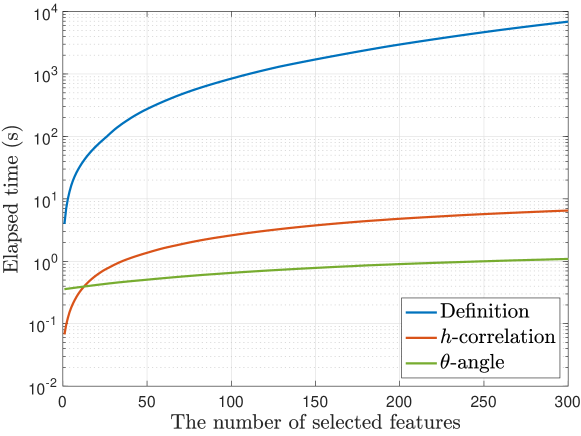
Figure 2: The elapsed time of the definition, $h$-correlation and $\theta$-angle-based feature selection methods.

5.2 Application to the real datasets

The three UCI datasets (Dua and Graff, 2019) and the MINST dataset (LeCun et al., 1998), which are summarised in Table 2, are used to compare the SSC with the seven MI-based criteria in classification tasks. The Lymph dataset (Michalski et al., 1986) is used to classify lymphography information into two classes, i.e. metastases and malign lymph, by 18 medical diagnostic attributes. The CNAE dataset (Ciarelli and Oliveira, 2009) is used to classify 1080 documents of business descriptions of Brazilian companies into nine economic activities by the frequencies of the 856 words in the documents. The Mfeat dataset (van Breukelen et al., 1998) is used to classify the handwritten numerals (i.e. 0 to 9) in a collection of Dutch utility maps by the 649 features extracted from the raw images. The NMIST dataset (LeCun et al., 1998) is used to classify the handwritten digits by the grey levels of the 784 pixels.

	Lymph	CNAE	Mfeat	NMIST
Data Type	Categorical & Discrete	Discrete	Continuous	Discrete
No. of Instances	142	1080	2000	700000
No. of Features	18	856	649	784
No. of Classes	2	9	10	10
Classifier	SVM	LDA	SVM	LDA

Table 2: An example of the greedy search based on the SSC.

For the SSC, the categorical features are transformed to an ordinal encoding, and the response variable is transformed to a $(c-1)$-label dummy encoding. For the MI-based criteria, the continuous features are discretised into five equal-width bins. Ten-fold cross validation is applied. Given the selected features, a linear Support Vector Machine (SVM) or a Linear Discriminant Analysis (LDA) model is trained with the training data, where the continuous features are standardised to z-scores. The performance of the feature selection criteria is evaluated by the averaged classification accuracy (ACC) on the validation data; the results are shown in Figure 3. Generally, the proposed SCC gives competitive results, whether the number of the selected features is small or large. When the ACC results are averaged over the number of selected features, the proposed SSC achieves the best results in three of the four datasets, as shown in Figure 3(e).

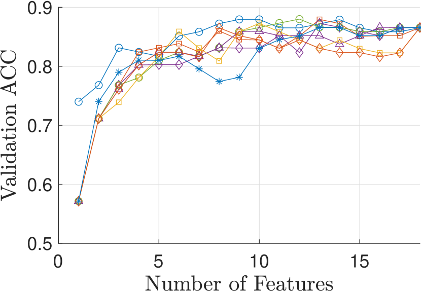
(a) Lymph

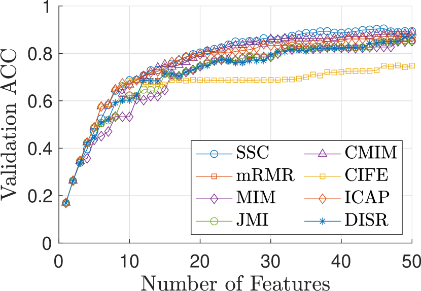
(b) CNAE

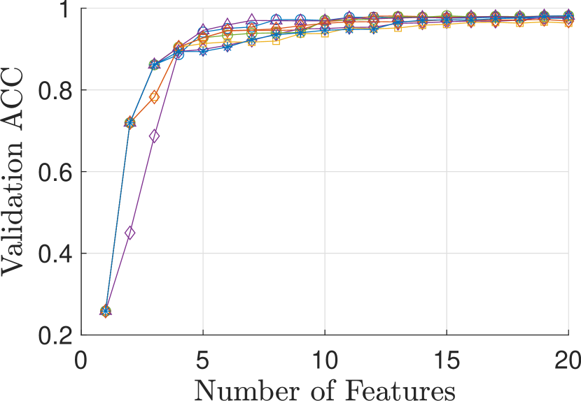
(c) Mfeat

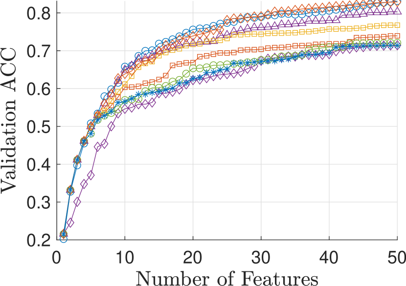
(d) NMIST

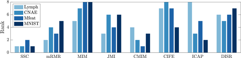
(e) Criterion rank

Figure 3: The comparison of the averaged ACC results between the different feature ranking criteria.

The four UCI datasets (Dua and Graff, 2019), which are summarised in Table 3, are used to compare the SSC with the seven MI-based criteria in linear regression tasks. The Student dataset (Cortez and Silva, 2008) is used to predict the final grade of the Portuguese class (from 0 to 20) in secondary education of two Portuguese schools by demographic, social and school-related features. The Parkinson dataset (Sakar et al., 2013) is used to predict the Unified Parkinson Disease Rating Scale (UPDRS) scores by the features extracted from multiple types of sound recordings, including sustained vowels, numbers, words and short sentences. The Conductor dataset (Hamidieh, 2018) is used in predicting the critical temperature of a superconductor from the features extracted from the superconductor’s chemical formula. The Energy dataset (Candanedo et al., 2017) is used to predict the energy usage of appliances during operation from environmental parameters. The original 24 features are expanded to 2924 features using 1st to 3rd-degree polynomial basis functions.

	Student	Parkinson	Conductor	Energy
Data Type	Categorical & Discrete	Continuous	Continuous	Continuous
No. of Instances	649	1040	21263	19735
No. of Features	30	26	81	2924

Table 3: An example of the greedy search based on the SSC.

Similar to the classification tasks, for the SSC, the categorical features are transformed to an ordinal encoding. For the MI-based criteria, the continuous features of the Energy dataset are discretised into ten equal-width bins, while the others are into five equal-width bins. Ten-fold cross validation is applied. Given the selected features, a Linear Regression (LR) model is fit to the training data, where the continuous features are standardised to z-scores. The performance of the feature selection criteria is evaluated by the averaged Root-Mean-Square Error (RMSE) on the validation data; the results are shown in Figure 4. The proposed SSC has an obvious advantage over the other criteria. As the four tasks are single-output regressions, the SSC degenerates to the coefficient of determination, which has a monotonically decreasing relationship with the RMSE of the LR model (Glantz et al., 2016). Therefore, the SSC-based filter method is equivalent to the LR-based wrapper method in the cases. In LR tasks, there is no surprise that the performance of the seven other filter methods is worse than the LR-based wrapper method.

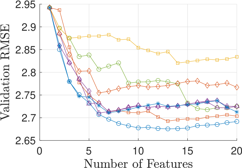
(a) Student

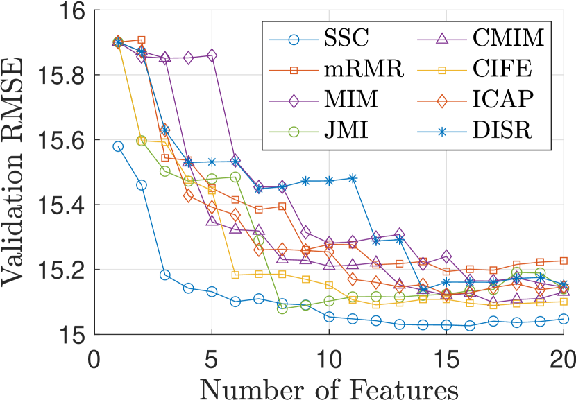
(b) Parkinson

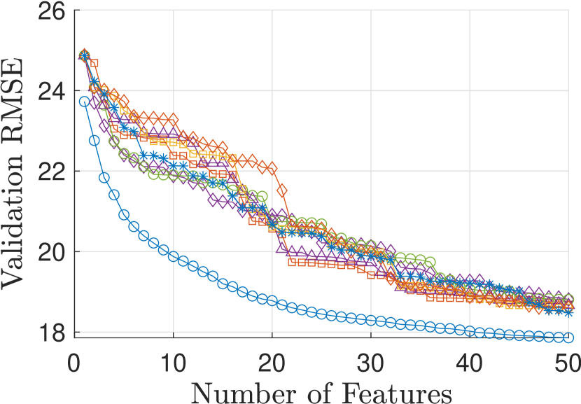
(c) Conductor

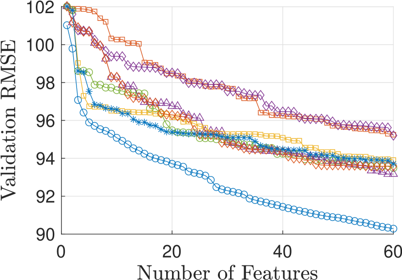
(d) Energy

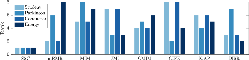
(e) Criterion rank

Figure 4: The comparison of the averaged RMSE results between the different feature ranking criteria.

6 Conclusions

This paper proposes a canonical-correlation-based fast feature selection method, which is composed of the $h$-correlation and $\theta$-angle-based methods. The $h$-correlation-based method boosts the computational speed when the number of features is large. The $\theta$-angle-based method boosts the computational speed when the number of instances is large. The supporting theorems for the proposed feature selection method have been developed to rigorously explain the theoretical reasons for the speed enhancement. The theorems are also fundamental to understand the CCA. The speed advantage of the proposed method has been demonstrated in the synthetic dataset. The comparison of feature ranking criteria shows the proposed SSC can give competitive results among the MI-based criteria, especially in regression tasks.

A Proof of the Correlation Superposition Theorem

Proof  The canonical correlation coefficient on the left-hand side of equation (6) is defined in (2). According to (3a), the sum of the squared canonical correlation coefficients, i.e. the sum of the eigenvalues, is given by,

$$\sum_{k=1}^{(p+q)\wedge m}R_{k}^{2}({\mathbf{X},\mathbf{Y}})=\tr{\left(\langle\mathbf{X}_{\mathrm{C}},\mathbf{X}_{\mathrm{C}}\rangle^{-1}\langle\mathbf{X}_{\mathrm{C}},\mathbf{Y}_{\mathrm{C}}\rangle\langle\mathbf{Y}_{\mathrm{C}},\mathbf{Y}_{\mathrm{C}}\rangle^{-1}\langle\mathbf{Y}_{\mathrm{C}},\mathbf{X}_{\mathrm{C}}\rangle\right)},$$ (14)

where the operator $\tr(\cdot)$ denotes the matrix trace, $\mathbf{X}=(\mathbf{X}_{\mathrm{s}},\mathbf{X}_{\mathrm{r}})$, and $\mathbf{X}_{\mathrm{C}}=(\mathbf{X}_{\mathrm{sC}},\mathbf{X}_{\mathrm{rC}})$. According to the assumptions T3.2 to T3.4, it can be found that,

$$\mathbf{Y}_{\mathrm{C}}=\mathbf{V}[\mathbf{Y}_{\mathrm{C}}]_{\mathbf{V}},$$

and,

$$\begin{split}\mathbf{X}_{\mathrm{C}}&=\mathbf{W}_{\mathrm{x}}[\mathbf{X}_{\mathrm{C}}]_{\mathbf{W}_{\mathrm{x}}}\\ &=\mathbf{W}_{\mathrm{x}}\left([\mathbf{X}_{\mathrm{sC}}]_{\mathbf{W}_{\mathrm{x}}},[\mathbf{X}_{\mathrm{rC}}]_{\mathbf{W}_{\mathrm{x}}}\right),\end{split}$$

where $\mathbf{W}_{\mathrm{x}}=(\mathbf{W}_{\mathrm{s}},\mathbf{W}_{\mathrm{r}})$ and,

$$[\mathbf{X}_{\mathrm{sC}}]_{\mathbf{W}_{\mathrm{x}}}=\begin{pmatrix}[\mathbf{X}_{\mathrm{sC}}]_{\mathbf{W}_{\mathrm{s}}}\\ \mathbf{0}_{q\times p}\\ \end{pmatrix}.$$

The right-hand side of (14) can then be rewritten as,

$$\begin{split}&\tr{\left(\langle\mathbf{X}_{\mathrm{C}},\mathbf{X}_{\mathrm{C}}\rangle^{-1}\langle\mathbf{X}_{\mathrm{C}},\mathbf{Y}_{\mathrm{C}}\rangle\langle\mathbf{Y}_{\mathrm{C}},\mathbf{Y}_{\mathrm{C}}\rangle^{-1}\langle\mathbf{Y}_{\mathrm{C}},\mathbf{X}_{\mathrm{C}}\rangle\right)}\\ =&\tr{\left([\mathbf{X}]_{\mathbf{W}_{\mathrm{x}}}^{-1}\langle\mathbf{W}_{\mathrm{x}},\mathbf{W}_{\mathrm{x}}\rangle^{-1}\langle\mathbf{W}_{\mathrm{x}},\mathbf{V}\rangle\langle\mathbf{V},\mathbf{V}\rangle^{-1}\langle\mathbf{V},\mathbf{W}_{\mathrm{x}}\rangle[\mathbf{X}]_{\mathbf{W}_{\mathrm{x}}}\right)}\\ =&\tr{\left(\langle\mathbf{W}_{\mathrm{x}},\mathbf{W}_{\mathrm{x}}\rangle^{-1}\langle\mathbf{W}_{\mathrm{x}},\mathbf{V}\rangle\langle\mathbf{V},\mathbf{V}\rangle^{-1}\langle\mathbf{V},\mathbf{W}_{\mathrm{x}}\rangle\right)}.\end{split}$$ (15)

As a result of,

$$\begin{split}\langle\mathbf{W}_{\mathrm{x}},\mathbf{W}_{\mathrm{x}}\rangle&=\begin{pmatrix}\langle\mathbf{W}_{\mathrm{s}},\mathbf{W}_{\mathrm{s}}\rangle&\mathbf{0}_{p\times q}\\ \mathbf{0}_{q\times p}&\langle\mathbf{W}_{\mathrm{r}},\mathbf{W}_{\mathrm{r}}\rangle\end{pmatrix}\\ \langle\mathbf{W}_{\mathrm{x}},\mathbf{V}\rangle&=\begin{pmatrix}\langle\mathbf{W}_{\mathrm{s}},\mathbf{V}\rangle\\ \langle\mathbf{W}_{\mathrm{r}},\mathbf{V}\rangle\end{pmatrix}\\ \langle\mathbf{V},\mathbf{W}_{\mathrm{x}}\rangle&=\big{(}\langle\mathbf{V},\mathbf{W}_{\mathrm{s}}\rangle,\langle\mathbf{V},\mathbf{W}_{\mathrm{r}}\rangle\big{)},\end{split}$$

and the columns of $\mathbf{W}_{\mathrm{s}}$, $\mathbf{W}_{\mathrm{r}}$ and $\mathbf{V}$ are zero-mean, it is found that (15) is equal to,

$$\begin{split}&\tr{\left(\langle\mathbf{W}_{\mathrm{s}},\mathbf{W}_{\mathrm{s}}\rangle^{-1}\langle\mathbf{W}_{\mathrm{s}},\mathbf{V}\rangle\langle\mathbf{V},\mathbf{V}\rangle^{-1}\langle\mathbf{V},\mathbf{W}_{\mathrm{s}}\rangle\right)}+\\ &\tr{\left(\langle\mathbf{W}_{\mathrm{r}},\mathbf{W}_{\mathrm{r}}\rangle^{-1}\langle\mathbf{W}_{\mathrm{r}},\mathbf{V}\rangle\langle\mathbf{V},\mathbf{V}\rangle^{-1}\langle\mathbf{V},\mathbf{W}_{\mathrm{r}}\rangle\right)}\\ =&\sum_{k=1}^{p\wedge m}R_{k}^{2}({\mathbf{W}_{\mathrm{s}},\mathbf{V}})+\sum_{k=1}^{q\wedge m}R_{k}^{2}({\mathbf{W}_{\mathrm{r}},\mathbf{V}}).\end{split}$$

Therefore, Theorem 3 follows.

 

B Proof of Lemma 5

Proof  According to the definition given by (2), the canonical correlation coefficient is given by,

$$\begin{split}R(\mathbf{X},\mathbf{Y})&\triangleq\max_{\bm{\upalpha},\bm{\upbeta}}r({\mathbf{X}_{\mathrm{C}}\bm{\upalpha},\mathbf{Y}_{\mathrm{C}}\bm{\upbeta}})\\ &=\max_{\bm{\upalpha,\upbeta}}\frac{\langle\mathbf{X}_{\mathrm{C}}\bm{\upalpha},\mathbf{Y}_{\mathrm{C}}\bm{\upbeta}\rangle}{\norm{\mathbf{X}_{\mathrm{C}}\bm{\upalpha}}\;\norm{\mathbf{Y}_{\mathrm{C}}\bm{\upbeta}}},\end{split}$$

where $\bm{\upalpha}\in\mathbb{R}^{n}$ and $\bm{\upbeta}\in\mathbb{R}^{m}$. From assumption L5.2, where,

$$\mathbf{X}_{\mathrm{C}} =\mathbf{U}[\mathbf{X}_{\mathrm{C}}]_{\mathbf{U}}$$

$$\mathbf{Y}_{\mathrm{C}} =\mathbf{U}[\mathbf{Y}_{\mathrm{C}}]_{\mathbf{U}}$$

$$\langle\mathbf{U},\mathbf{U}\rangle =I_{z},$$

it can be seen that,

$$\begin{split}\max_{\bm{\upalpha},\bm{\upbeta}}\frac{\langle\mathbf{X}_{\mathrm{C}}\bm{\upalpha},\mathbf{Y}_{\mathrm{C}}\bm{\upbeta}\rangle}{\norm{\mathbf{X}_{\mathrm{C}}\bm{\upalpha}}\;\norm{\mathbf{Y}_{\mathrm{C}}\bm{\upbeta}}}&=\max_{\bm{\upalpha},\bm{\upbeta}}\frac{\langle\mathbf{U}[\mathbf{X}_{\mathrm{C}}]_{\mathbf{U}}\bm{\upalpha},\mathbf{U}[\mathbf{Y}_{\mathrm{C}}]_{\mathbf{U}}\bm{\upbeta}\rangle}{\norm{\mathbf{U}[\mathbf{X}_{\mathrm{C}}]_{\mathbf{U}}\bm{\upalpha}}\;\norm{\mathbf{U}[\mathbf{Y}_{\mathrm{C}}]_{\mathbf{U}}\bm{\upbeta}}}\\ &=\max_{\bm{\upalpha},\bm{\upbeta}}\frac{\langle[\mathbf{X}_{\mathrm{C}}]_{\mathbf{U}}\bm{\upalpha},[\mathbf{Y}_{\mathrm{C}}]_{\mathbf{U}}\bm{\upbeta}\rangle}{\norm{[\mathbf{X}_{\mathrm{C}}]_{\mathbf{U}}\bm{\upalpha}}\;\norm{[\mathbf{Y}_{\mathrm{C}}]_{\mathbf{U}}\bm{\upbeta}}}\\ &=\max_{\bm{\upalpha},\bm{\upbeta}}\cos\left({\angle([\mathbf{X}_{\mathrm{C}}]_{\mathbf{U}}\bm{\upalpha},[\mathbf{Y}_{\mathrm{C}}]_{\mathbf{U}}\bm{\upbeta})}\right)\\ &=\cos\left({\min_{\bm{\upalpha},\bm{\upbeta}}\angle([\mathbf{X}_{\mathrm{C}}]_{\mathbf{U}}\bm{\upalpha},[\mathbf{Y}_{\mathrm{C}}]_{\mathbf{U}}\bm{\upbeta})}\right)\\ &=\cos\big{(}\varTheta([\mathbf{X}_{\mathrm{C}}]_{\mathbf{U}},[\mathbf{Y}_{\mathrm{C}}]_{\mathbf{U}})\big{)}.\end{split}$$

Thus, Lemma 5 is proved.

 

C Proof of the Angle Superposition Theorem

Proof  According to Lemma 5, the canonical correlation coefficients on the left-hand side of (9) can be computed via (4), where the optimal vectors $\bm{\upalpha}\in\mathbb{R}^{p+q}$ and $\bm{\upbeta}\in\mathbb{R}^{m}$ are obtained by solving the eigenvalue problem given by,

$$\langle[\mathbf{X}_{\mathrm{C}}]_{\mathbf{U}},[\mathbf{X}_{\mathrm{C}}]_{\mathbf{U}}\rangle^{-1}\langle[\mathbf{X}_{\mathrm{C}}]_{\mathbf{U}},[\mathbf{Y}_{\mathrm{C}}]_{\mathbf{U}}\rangle\langle[\mathbf{Y}_{\mathrm{C}}]_{\mathbf{U}},[\mathbf{Y}_{\mathrm{C}}]_{\mathbf{U}}\rangle^{-1}\langle[\mathbf{Y}_{\mathrm{C}}]_{\mathbf{U}},[\mathbf{X}_{\mathrm{C}}]_{\mathbf{U}}\rangle\bm{\upalpha} =R^{2}({\mathbf{X},\mathbf{Y}})\bm{\upalpha}$$ (17a)

$$\langle[\mathbf{Y}_{\mathrm{C}}]_{\mathbf{U}},[\mathbf{Y}_{\mathrm{C}}]_{\mathbf{U}}\rangle^{-1}\langle[\mathbf{Y}_{\mathrm{C}}]_{\mathbf{U}},[\mathbf{X}_{\mathrm{C}}]_{\mathbf{U}}\rangle\langle[\mathbf{X}_{\mathrm{C}}]_{\mathbf{U}},[\mathbf{X}_{\mathrm{C}}]_{\mathbf{U}}\rangle^{-1}\langle[\mathbf{X}_{\mathrm{C}}]_{\mathbf{U}},[\mathbf{Y}_{\mathrm{C}}]_{\mathbf{U}}\rangle\bm{\upbeta} =R^{2}({\mathbf{X},\mathbf{Y}})\bm{\upbeta},$$ (17b)

where $\mathbf{X}=(\mathbf{X}_{\mathrm{s}},\mathbf{X}_{\mathrm{r}})$ and $\mathbf{X}_{\mathrm{C}}=(\mathbf{X}_{\mathrm{sC}},\mathbf{X}_{\mathrm{rC}})$. According to (17a), the sum of the squared canonical correlation coefficients, i.e. the sum of the eigenvalues, is given by,

$$\begin{split}&\sum_{k=1}^{(p+q)\wedge m}R_{k}^{2}({\mathbf{X},\mathbf{Y}})\\ =&\tr{\left(\langle[\mathbf{X}_{\mathrm{C}}]_{\mathbf{U}},[\mathbf{X}_{\mathrm{C}}]_{\mathbf{U}}\rangle^{-1}\langle[\mathbf{X}_{\mathrm{C}}]_{\mathbf{U}},[\mathbf{Y}_{\mathrm{C}}]_{\mathbf{U}}\rangle\langle[\mathbf{Y}_{\mathrm{C}}]_{\mathbf{U}},[\mathbf{Y}_{\mathrm{C}}]_{\mathbf{U}}\rangle^{-1}\langle[\mathbf{Y}_{\mathrm{C}}]_{\mathbf{U}},[\mathbf{X}_{\mathrm{C}}]_{\mathbf{U}}\rangle\right)}.\end{split}$$ (18)

According to the assumptions T6.3 to T6.5, it can be found that,

$$[\mathbf{Y}_{\mathrm{C}}]_{\mathbf{U}}=\mathbf{V}\big{[}[\mathbf{Y}_{\mathrm{C}}]_{\mathbf{U}}\big{]}_{\mathbf{V}},$$

and,

$$\begin{split}[\mathbf{X}_{\mathrm{C}}]_{\mathbf{U}}&=\mathbf{W}_{\mathrm{x}}\big{[}[\mathbf{X}_{\mathrm{C}}]_{\mathbf{U}}\big{]}_{\mathbf{W}_{\mathrm{x}}}\\ &=\mathbf{W}_{\mathrm{x}}\left(\big{[}[\mathbf{X}_{\mathrm{sC}}]_{\mathbf{U}}\big{]}_{\mathbf{W}_{\mathrm{x}}},\big{[}[\mathbf{X}_{\mathrm{rC}}]_{\mathbf{U}}\big{]}_{\mathbf{W}_{\mathrm{x}}}\right),\end{split}$$

where $\mathbf{W}_{\mathrm{x}}=(\mathbf{W}_{\mathrm{s}},\mathbf{W}_{\mathrm{r}})$ and,

$$\big{[}[\mathbf{X}_{\mathrm{sC}}]_{\mathbf{U}}\big{]}_{\mathbf{W}_{\mathrm{x}}}=\begin{pmatrix}\big{[}[\mathbf{X}_{\mathrm{sC}}]_{\mathbf{U}}\big{]}_{\mathbf{W}_{\mathrm{s}}}\\ \mathbf{0}_{q\times p}\\ \end{pmatrix}.$$

Then, the right-hand side of (18) can be rewritten as,

$$\begin{split}&\tr{\left(\langle[\mathbf{X}_{\mathrm{C}}]_{\mathbf{U}},[\mathbf{X}_{\mathrm{C}}]_{\mathbf{U}}\rangle^{-1}\langle[\mathbf{X}_{\mathrm{C}}]_{\mathbf{U}},[\mathbf{Y}_{\mathrm{C}}]_{\mathbf{U}}\rangle\langle[\mathbf{Y}_{\mathrm{C}}]_{\mathbf{U}},[\mathbf{Y}_{\mathrm{C}}]_{\mathbf{U}}\rangle^{-1}\langle[\mathbf{Y}_{\mathrm{C}}]_{\mathbf{U}},[\mathbf{X}_{\mathrm{C}}]_{\mathbf{U}}\rangle\right)}\\ =&\tr{\left(\big{[}[\mathbf{X}_{\mathrm{C}}]_{\mathbf{U}}\big{]}_{\mathbf{W}_{\mathrm{x}}}^{-1}\langle\mathbf{W}_{\mathrm{x}},\mathbf{W}_{\mathrm{x}}\rangle^{-1}\langle\mathbf{W}_{\mathrm{x}},\mathbf{V}\rangle\langle\mathbf{V},\mathbf{V}\rangle^{-1}\langle\mathbf{V},\mathbf{W}_{\mathrm{x}}\rangle\big{[}[\mathbf{X}_{\mathrm{C}}]_{\mathbf{U}}\big{]}_{\mathbf{W}_{\mathrm{x}}}\right)}\\ =&\tr{\left(\langle\mathbf{W}_{\mathrm{x}},\mathbf{W}_{\mathrm{x}}\rangle^{-1}\langle\mathbf{W}_{\mathrm{x}},\mathbf{V}\rangle\langle\mathbf{V},\mathbf{V}\rangle^{-1}\langle\mathbf{V},\mathbf{W}_{\mathrm{x}}\rangle\right)}.\end{split}$$ (19)

Because,

$$\begin{split}\langle\mathbf{W}_{\mathrm{x}},\mathbf{W}_{\mathrm{x}}\rangle&=\begin{pmatrix}\langle\mathbf{W}_{\mathrm{s}},\mathbf{W}_{\mathrm{s}}\rangle&\mathbf{0}_{p\times q}\\ \mathbf{0}_{q\times p}&\langle\mathbf{W}_{\mathrm{r}},\mathbf{W}_{\mathrm{r}}\rangle\end{pmatrix}\\ \langle\mathbf{W}_{\mathrm{x}},\mathbf{V}\rangle&=\begin{pmatrix}\langle\mathbf{W}_{\mathrm{s}},\mathbf{V}\rangle\\ \langle\mathbf{W}_{\mathrm{r}},\mathbf{V}\rangle\end{pmatrix}\\ \langle\mathbf{V},\mathbf{W}_{\mathrm{x}}\rangle&=\big{(}\langle\mathbf{V},\mathbf{W}_{\mathrm{s}}\rangle,\langle\mathbf{V},\mathbf{W}_{\mathrm{r}}\rangle\big{)},\end{split}$$

it is found that (19) is equal to,

$$\begin{split}&\tr{\left(\langle\mathbf{W}_{\mathrm{s}},\mathbf{W}_{\mathrm{s}}\rangle^{-1}\langle\mathbf{W}_{\mathrm{s}},\mathbf{V}\rangle\langle\mathbf{V},\mathbf{V}\rangle^{-1}\langle\mathbf{V},\mathbf{W}_{\mathrm{s}}\rangle\right)}+\\ &\tr{\left(\langle\mathbf{W}_{\mathrm{r}},\mathbf{W}_{\mathrm{r}}\rangle^{-1}\langle\mathbf{W}_{\mathrm{r}},\mathbf{V}\rangle\langle\mathbf{V},\mathbf{V}\rangle^{-1}\langle\mathbf{V},\mathbf{W}_{\mathrm{r}}\rangle\right)}\\ =&\sum_{k=1}^{p\wedge m}\cos^{2}\big{(}\varTheta_{k}(\mathbf{W}_{\mathrm{s}},\mathbf{V})\big{)}+\sum_{k=1}^{q\wedge m}\cos^{2}\big{(}\varTheta_{k}({\mathbf{W}_{\mathrm{r}},\mathbf{V}})\big{)}.\end{split}$$

and Theorem 6 follows.

 

D An illustration of the canonical-correlation-based fast feature selection

The seven instances from the Fisher’s iris dataset (Fisher, 1936) are given in Table 4, including four features and three classes. The objective of the feature selection is to find three useful features for the three-species classification.

Sepal Length	Sepal Width	Petal Length	Petal Width	Species
5.1	3.5	1.4	0.2	setosa
4.9	3	1.4	0.2	setosa
7	3.2	4.7	1.4	versicolor
6.4	3.2	4.5	1.5	versicolor
6.3	3.3	6	2.5	virginica
5.8	2.7	5.1	1.9	virginica
7.1	3	5.9	2.1	virginica

Table 4: Fisher’s Iris Dataset Sample.

The feature matrix is given by,

$$\mathbf{X}=\left(\mathbf{x}_{1},\mathbf{x}_{2},\mathbf{x}_{3},\mathbf{x}_{4}\right)=\begin{pmatrix}5.1&4.9&7&6.4&6.3&5.8&7.1\\ 3.5&3&3.2&3.2&3.3&2.7&3\\ 1.4&1.4&4.7&4.5&6&5.1&5.9\\ 0.2&0.2&1.4&1.5&2.5&1.9&2.1\\ \end{pmatrix}^{\top},$$

and the $(c-1)$-label dummy encoded response is,

$$\mathbf{Y}=\begin{pmatrix}1&1&0&0&0&0&0\\ 0&0&1&1&0&0&0\\ \end{pmatrix}^{\top},$$

where $(1,0)$ represents setosa, $(0,1)$ represents versicolor, and $(0,0)$ represents virginica. Therefore, let $N=7$, $n=4$, and $m=2$. Following the algorithm introduced in Section 4.1, the procedure of the fast canonical-correlation-based feature selection method is shown below.

Step 1. First, centre $\mathbf{X}$ into $\mathbf{X}_{\mathrm{C}}$, which is given by,

$$\mathbf{X}_{\mathrm{C}}=\begin{pmatrix}-0.9857&-1.1857&0.9143&0.3143&0.2143&-0.2857&1.0143\\ 0.3714&-0.1286&0.0714&0.0714&0.1714&-0.4286&-0.1286\\ -2.7429&-2.7429&0.5571&0.3571&1.8571&0.9571&1.7571\\ -1.2000&-1.2000&0.0000&0.1000&1.1000&0.5000&0.7000\\ \end{pmatrix}^{\top}.$$

Second, centre $\mathbf{Y}$ into $\mathbf{Y}_{\mathrm{C}}$, which is given by,

$$\mathbf{Y}_{\mathrm{C}}=\begin{pmatrix}0.7143&0.7143&-0.2857&-0.2857&-0.2857&-0.2857&-0.2857\\ -0.2857&-0.2857&0.7143&0.7143&-0.2857&-0.2857&-0.2857\\ \end{pmatrix}^{\top}.$$

Step 2. As $N>n+m$, let $\mathbf{F}_{\mathrm{X}}=[\mathbf{X}_{\mathrm{C}}]_{\mathbf{U}}$ and $\mathbf{F}_{\mathrm{Y}}=[\mathbf{Y}_{\mathrm{C}}]_{\mathbf{U}}$, where,

$$\mathbf{F}_{\mathrm{X}}=\begin{pmatrix}1.8286&-0.9433&0.4666&-0.1315&-0.0102&0.0041\\ -0.1782&-0.2150&0.2037&0.5233&0.0306&-0.0016\\ 4.7824&0.2504&-0.0530&-0.0040&0.0116&-0.0086\\ 2.1445&0.4445&-0.0823&0.1837&-0.0543&0.0111\\ \end{pmatrix}^{\top},$$

$$\mathbf{F}_{\mathrm{Y}}=\begin{pmatrix}-1.1535&0.1772&0.2389&0.0557&-0.0799&-0.0090\\ 0.2424&-1.0723&-0.4584&0.0952&-0.0301&-0.0022\\ \end{pmatrix}^{\top}.$$

Here, the orthonormal basis forming $\mathbf{U}$ is obtained by SVD of the matrix $(\mathbf{X}_{\mathrm{C}},\mathbf{Y}_{\mathrm{C}})$, and $\mathbf{U}$ is given by,

$$\mathbf{U}=\begin{pmatrix}-0.5724&-0.5810&0.1497&0.0927&0.3680&0.1695&0.3736\\ 0.0263&0.1509&-0.6540&-0.4183&0.4083&0.4540&0.0327\\ 0.3015&-0.0626&0.0298&-0.4881&0.0159&-0.4662&0.6697\\ 0.3769&-0.3212&-0.0979&0.1931&0.6321&-0.4206&-0.3625\\ 0.5397&-0.6196&0.0554&-0.0855&-0.3155&0.4621&-0.0366\\ 0.0668&-0.0759&-0.6273&0.6251&-0.2359&-0.1207&0.3679\\ \end{pmatrix}^{\top}.$$

Then, the classical Gram-Schmidt process is applied to $\mathbf{F}_{\mathrm{Y}}$ to obtain $\mathbf{V}$, that is,

$$\mathbf{V}=\begin{pmatrix}-1.1535&0.1772&0.2389&0.0557&-0.0799&-0.0090\\ -0.2190&-1.0014&-0.3628&0.1175&-0.0621&-0.0058\\ \end{pmatrix}^{\top}.$$

Step 3. In this step, as no feature has been selected, $\mathbf{X}_{\mathrm{s}}$ is empty and $\mathbf{X}_{\mathrm{r}}$ is the same as $\mathbf{X}$. Correspondingly, $\mathbf{F}_{\mathrm{Xs}}$ is empty and $\mathbf{F}_{\mathrm{Xr}}$ is the same as $\mathbf{F}_{\mathrm{X}}$. As no $\mathbf{W}_{\mathrm{s}}$ that the $\mathbf{F}_{\mathrm{Xr}}$ is orthogonalised to, let $\mathbf{W}_{\mathrm{r}}=\mathbf{F}_{\mathrm{Xr}}$.

Step 4. The angle between $\mathbf{w}_{\mathrm{r}i}$ and $\mathbf{V}$ are evaluated by,

$$\begin{split}\cos^{2}\big{(}\varTheta({\mathbf{w}_{\mathrm{r}1},\mathbf{V}})\big{)}=\theta_{1,1}+\theta_{1,2}=0.7386+0.0242&=0.7628\\ \cos^{2}\big{(}\varTheta({\mathbf{w}_{\mathrm{r}2},\mathbf{V}})\big{)}=\theta_{2,1}+\theta_{2,2}=0.1047+0.1217&=0.2264\\ \cos^{2}\big{(}\varTheta({\mathbf{w}_{\mathrm{r}3},\mathbf{V}})\big{)}=\theta_{3,1}+\theta_{3,2}=0.9184+0.0595&=0.9779\\ \cos^{2}\big{(}\varTheta({\mathbf{w}_{\mathrm{r}4},\mathbf{V}})\big{)}=\theta_{4,1}+\theta_{4,2}=0.8331+0.1273&=0.9604.\end{split}$$ (20)

Step 5. The third feature (i.e. petal length) has the highest cosine of the angle. Thus, the petal length is selected into $\mathbf{X}_{\mathrm{s}}$, and the rest of the features contained in $\mathbf{X}_{\mathrm{r}}$ in order are sepal length, sepal width, and petal width.

Step 3. According to the new $\mathbf{X}_{\mathrm{s}}$ and $\mathbf{X}_{\mathrm{r}}$, divide $\mathbf{F}_{\mathrm{X}}$ into $(\mathbf{F}_{\mathrm{Xs}},\mathbf{F}_{\mathrm{Xr}})$ again. As $\mathbf{F}_{\mathrm{Xs}}$ only has one column, let,

$$\mathbf{W}_{\mathrm{s}}=\mathbf{F}_{\mathrm{Xs}}=\begin{pmatrix}4.7824&0.2504&-0.0530&-0.0040&0.0116&-0.0086\\ \end{pmatrix}^{\top}.$$ (21)

Through the classical Gram-Schmidt process, $\mathbf{F}_{\mathrm{Xr}}$ can be orthogonalised to $\mathbf{W}_{\mathrm{s}}$, which is given by,

$$\mathbf{W}_{\mathrm{r}}=\begin{pmatrix}0.0596&-1.0359&0.4862&-0.1300&-0.0145&0.0073\\ 0.0133&-0.2049&0.2016&0.5232&0.0310&-0.0019\\ -0.0177&0.3313&-0.0584&0.1855&-0.0595&0.0150\\ \end{pmatrix}^{\top}.$$ (22)

Step 4. The angle between $\mathbf{w}_{\mathrm{r}i}$ and $\mathbf{V}$ are evaluated by,

$$\begin{split}\cos^{2}\big{(}\varTheta({\mathbf{w}_{\mathrm{r}1},\mathbf{V}})\big{)}=\theta_{1,1}+\theta_{1,2}=0.0107+0.4352&=0.4458\\ \cos^{2}\big{(}\varTheta({\mathbf{w}_{\mathrm{r}2},\mathbf{V}})\big{)}=\theta_{2,1}+\theta_{2,2}=0.0011+0.0830&=0.0841\\ \cos^{2}\big{(}\varTheta({\mathbf{w}_{\mathrm{r}3},\mathbf{V}})\big{)}=\theta_{3,1}+\theta_{3,2}=0.0296+0.4348&=0.4644.\end{split}$$ (23)

Step 5. The third feature (i.e. petal width) has the highest cosine of the angle. Thus, the features contained in $\mathbf{X}_{\mathrm{s}}$ in order are petal length and petal width, and the features contained in $\mathbf{X}_{\mathrm{r}}$ in order are sepal length and sepal width.

Step 3. According to the new $\mathbf{X}_{\mathrm{s}}$ and $\mathbf{X}_{\mathrm{r}}$, divide $\mathbf{F}_{\mathrm{X}}$ into $(\mathbf{F}_{\mathrm{Xs}},\mathbf{F}_{\mathrm{Xr}})$ again. The matrix $\mathbf{W}_{\mathrm{s}}$ is formed by appending the third column of (22) to (21), which is given by,

$$\mathbf{W}_{\mathrm{s}}=\begin{pmatrix}4.7824&0.2504&-0.0530&-0.0040&0.0116&-0.0086\\ -0.0177&0.3313&-0.0584&0.1855&-0.0595&0.0150\\ \end{pmatrix}^{\top}.$$

Through the classical Gram-Schmidt process, each column of $\mathbf{F}_{\mathrm{Xr}}$ is orthogonalised to $\mathbf{W}_{\mathrm{s}}$, respectively, to obtain $\mathbf{W}_{\mathrm{r}}$, that is,

$$\mathbf{W}_{\mathrm{r}}=\begin{pmatrix}0.0135&-0.1714&0.3339&0.3541&-0.1698&0.0463\\ 0.0151&-0.2383&0.2075&0.5045&0.0370&-0.0034\\ \end{pmatrix}^{\top}.$$

Step 4. The angle between $\mathbf{w}_{\mathrm{r}i}$ and $\mathbf{V}$ are evaluated by,

$$\begin{split}\cos^{2}\big{(}\varTheta({\mathbf{w}_{\mathrm{r}1},\mathbf{V}})\big{)}=\theta_{1,1}+\theta_{1,2}=0.0105+0.0277&=0.0382\\ \cos^{2}\big{(}\varTheta({\mathbf{w}_{\mathrm{r}2},\mathbf{V}})\big{)}=\theta_{2,1}+\theta_{2,2}=0.0004+0.1103&=0.1108.\end{split}$$ (24)

Step 5. The second feature (i.e. sepal width), which has the highest cosine of the angle, is selected into $\mathbf{X}_{\mathrm{s}}$. Therefore, the 3 selected features are petal length, petal width, and sepal width.

The squared canonical correlation coefficients between the 3 features and $\mathbf{Y}$ are given by,

$$\begin{split}R_{1}^{2}({(\mathbf{x}_{3},\mathbf{x}_{4},\mathbf{x}_{2}),\mathbf{Y}})&=0.9905\\ R_{2}^{2}({(\mathbf{x}_{3},\mathbf{x}_{4},\mathbf{x}_{2}),\mathbf{Y}})&=0.5626.\end{split}$$

To verify the equality between the squared canonical correlation coefficients and $\theta$-angle in the Minimum Angle Theorem, the left-hand side of (10) is given by,

$$\begin{split}R_{1}^{2}({(\mathbf{x}_{3},\mathbf{x}_{4},\mathbf{x}_{2}),\mathbf{Y}})+R_{2}^{2}({(\mathbf{x}_{3},\mathbf{x}_{4},\mathbf{x}_{2}),\mathbf{Y}})&=0.9905+0.5626\\ &=1.5531,\end{split}$$

and the right-hand side of (10) is given by the sum of the maxima in (20), (23) and (24), that is $0.9779+0.4644+0.1108=1.5531$.

References

- Brown et al. (2012) Gavin Brown, Adam Pocock, Ming-Jie Zhao, and Mikel Luján. Conditional likelihood maximisation: a unifying framework for information theoretic feature selection. Journal of Machine Learning Research, 13(1):27–66, 2012.
- Candanedo et al. (2017) Luis M. Candanedo, Véronique Feldheim, and Dominique Deramaix. Data driven prediction models of energy use of appliances in a low-energy house. Energy and Buildings, 140:81–97, 2017.
- Ciarelli and Oliveira (2009) Patrick M. Ciarelli and Elias Oliveira. Agglomeration and elimination of terms for dimensionality reduction. In 2009 Ninth International Conference on Intelligent Systems Design and Applications, pages 547–552. IEEE, 2009.
- Cohen et al. (2003) Jacob Cohen, Patricia Cohen, Stephen G. West, and Leona S. Aiken. Applied Multiple Regression/Correlation Analysis for the Behavioral Sciences. Taylor & Francis, Mahwah, NJ, USA, 3rd edition, 2003.
- Cormen et al. (2009) Thomas H. Cormen, Charles E. Leiserson, Ronald L. Rivest, and Clifford Stein. Introduction to Algorithms. MIT Press, Cambridge, MA, USA, 3rd edition, 2009.
- Cortez and Silva (2008) Paulo Cortez and Alice M. G. Silva. Using data mining to predict secondary school student performance. In Proceedings of the Fifth Future Business Technology Conference, pages 5–12. EUROSIS-ETI, 2008.
- Dua and Graff (2019) Dheeru Dua and Casey Graff. UCI machine learning repository, 2019. URL http://archive.ics.uci.edu/ml.
- Fisher (1936) Ronald A. Fisher. The use of multiple measurements in taxonomic problems. Annals of Eugenics, 7(2):179–188, 1936.
- Glantz et al. (2016) Stanton A. Glantz, Bryan K. Slinker, and Torsten B. Neilands. Primer of Applied Regression & Analysis of Variance. McGraw-Hill Education, New York City, NY, USA, 3rd edition, 2016.
- Golub and Van Loan (2013) Gene H. Golub and Charles F. Van Loan. Matrix Computations. Johns Hopkins University Press, Baltimore, MD, USA, 4th edition, 2013.
- Guyon and Elisseeff (2003) Isabelle Guyon and André Elisseeff. An introduction to variable and feature selection. Journal of Machine Learning Research, 3:1157–1182, 2003.
- Hall and Smith (1999) Mark A. Hall and Lloyd A. Smith. Feature selection for machine learning: Comparing a correlation-based filter approach to the wrapper. In Proceedings of the Twelfth International Florida Artificial Intelligence Research Society Conference, page 235–239. AAAI Press, 1999.
- Hamidieh (2018) Kam Hamidieh. A data-driven statistical model for predicting the critical temperature of a superconductor. Computational Materials Science, 154:346–354, 2018.
- Hanchuan Peng et al. (2005) Hanchuan Peng, Fuhui Long, and Chris Ding. Feature selection based on mutual information criteria of max-dependency, max-relevance, and min-redundancy. IEEE Transactions on Pattern Analysis and Machine Intelligence, 27(8):1226–1238, 2005.
- Hardoon et al. (2004) David R. Hardoon, Sandor Szedmak, and John Shawe-Taylor. Canonical correlation analysis: An overview with application to learning methods. Neural Computation, 16(12):2639–2664, 2004.
- Hotelling (1936) Harold Hotelling. Relations between two sets of variates. Biometrika, 28(3/4):321–377, 1936.
- Kaya et al. (2014) Heysem Kaya, Florian Eyben, Albert A. Salah, and Björn Schuller. CCA based feature selection with application to continuous depression recognition from acoustic speech features. In 2014 IEEE International Conference on Acoustics, Speech and Signal Processing, pages 3729–3733. IEEE, 2014.
- LeCun et al. (1998) Yann LeCun, Léon Bottou, Yoshua Bengio, and Patrick Haffner. Gradient-based learning applied to document recognition. Proceedings of the IEEE, 86(11):2278–2324, 1998.
- Li et al. (2017) Yun Li, Tao Li, and Huan Liu. Recent advances in feature selection and its applications. Knowledge and Information Systems, 53(3):551–577, 2017.
- Michalski et al. (1986) Ryszard S. Michalski, Igor Mozetic, Jiarong Hong, and Nada Lavrac. The multi-purpose incremental learning system AQ15 and its testing application to three medical domains. In Proceedings of the Fifth National Conference on Artificial Intelligence, pages 1041–1045, 1986.
- Sakar et al. (2013) Betul Erdogdu Sakar, M. Erdem Isenkul, C. Okan Sakar, Ahmet Sertbas, Fikret Gurgen, Sakir Delil, Hulya Apaydin, and Olcay Kursun. Collection and analysis of a Parkinson speech dataset with multiple types of sound recordings. IEEE Journal of Biomedical and Health Informatics, 17(4):828–834, 2013.
- Tibshirani (1996) Robert Tibshirani. Regression shrinkage and selection via the lasso. Journal of the Royal Statistical Society: Series B (Methodological), 58(1):267–288, 1996.
- van Breukelen et al. (1998) Martijn van Breukelen, Robert P. W. Duin, David M. J. Tax, and Janneke E. den Hartog. Handwritten digit recognition by combined classifiers. Kybernetika, 34(4):381–386, 1998.
- Zhang and Lang (2021) Sikai Zhang and Zi-Qiang Lang. Orthogonal least squares based fast feature selection for linear classification, 2021. arXiv:2101.08539 [cs.LG].