Graphene quantum dots with Stone-Wales defect as a topologically tunable platform for visible-light harvesting

Abstract

In this work, we report for the first time the crucial role of topological anomalies like Stone-Wales (SW) type bond rotations in tuning the optical properties of graphene quantum dots (GQDs). By means of first-principles calculations, we first show that the structural stability of GQDs strongly depends on position of SW defects. Optical absorption spectra is then computed using electron-correlated methodology to demonstrate that SW type reconstruction is responsible for the appearance of new defect-induced peaks below the optical gap and dramatically modifies the optical absorption profile. In addition, our investigations signify that electron correlation effects become more dominant for SW-defected GQDs. We finally establish that the introduction of SW defects at specific locations strongly enhances light absorption in visible range, which is of prime importance for designing light harvesting, photocatalytic and optoelectronic devices.

I Introduction

Currently, the contribution of solar energy to the total global energy demand is quite low and consequently tremendous scientific efforts have been directed to efficiently design devices for visible light harvesting. In recent years, graphene quantum dots have emerged as a promising solution for developing different optoelectronic devices, bio-imaging sensors, etc. due to their unique electronic and tunable optical properties (Wang et al., 2016). Despite this recent progress, very little literature exists on the potential application of GQDs in visible light-sensitive devices since most of the GQDs are efficient absorbers of light in the UV range, rather than the visible range. In this work, we demonstrate for the first time that systematic introduction of topological disorders such as Stone-Wales defects in GQDs in a controlled manner can significantly enhance light absorption in the visible range, opening up their prospective applications in the field of photovoltaics.

The SW defect formed due to rotation of carbon-carbon bonds with respect to their midpoint by 90⁰, leading to the transformation of four hexagons into two pentagons and two heptagons, has attracted substantial attention as it has the lowest formation energy among the different types of topological anomalies in graphenic systems. Experimental investigations have demonstrated the existence of SW-type bond rotations along the edge (He et al., 2015; Girit et al., 2009; Chuvilin et al., 2009) and also in the core (Meyer et al., 2008) of graphene and its nano-structures. The presence of SW defects along the zigzag boundary leads to the formation of a reconstructed zigzag edge (reczag edge) which is experimentally confirmed to be stable in single-walled carbon nanotube for a time span of several seconds (Koskinen et al., 2009). The sequential reconstruction of zigzag edge of GNRs into reczag edge as a function of time and temperature has also been investigated theoretically (Lee et al., 2010). Theoretical studies indicate that energy stability of different edge configurations is a highly debated issue, with critical dependence on the dimension of graphene nanostructures and concentration of hydrogen atoms (Koskinen et al., 2008; Wassmann et al., 2008; Voznyy et al., 2011). Inspite of availability of substantial amount of literature to demonstrate the existence of SW defects and its consequence on the electronic, magnetic and mechanical properties of graphene nanostructures (Bhowmick and Waghmare, 2010; Romanovsky et al., 2012; Rodrigues et al., 2011; Ihnatsenka and Kirczenow, 2013), no studies have been initiated till date to the best of our knowledge, to explore the influence of these defects on the optical properties of these systems.

In the present work, we have studied the structure, energetics, and optical properties of the SW type reconstructions in a reasonably large hydrogen-passivated graphene quantum dot with 64 carbon atoms (GQD-64). We considered two locations for the SW defect: (i) one of the zigzag edges resulting in a reczag edge (SW1-GQD-64), and (ii) core of GQD-64 (SW2-GQD-64), and employed a first-principles methodology to probe their energetics. For computing their optical properties, we used a computational approach based on the Pariser-Parr-Pople (PPP) model Hamiltonian, coupled with the configuration-interaction (CI) methodology for including the electron-correlation effects. Our studies reveal that the introduction of SW-type defects in GQDs significantly alters their electronic structure and optical properties as compared to those of the pristine system. Furthermore, our results demonstrate that the striking attributes of these properties are critically dependent upon the location of SW-type defects.

The rest of the paper is organized as follows. The computational methodology employed by us is briefly described in Sec. II which is followed by the results and discussion in Sec. III. Finally, the conclusions are presented in Sec. IV.

II Computational Methodology

The schematic representations of hydrogen-passivated GQD-64, SW1-GQD-64 and SW2-GQD-64, lying in the x-y plane, are given in Fig. 1. The bond-lengths and bond-angles between carbon atoms are chosen uniformly as 1.4 Å and $120^{0}$, respectively, for GQD-64. In case of SW1-GQD-64 and SW2-GQD-64 configurations, the optimized geometries obtained with Gaussian 16 program package(Frisch et al., 2016) using cc-pvdz basis set at restricted Hartree-Fock (RHF) level, exhibit non-uniform C-C bond-lengths in the range (1.35 - 1.49) Å. The correlated computations on these relaxed geometries have been performed by employing our theoretical formalism based upon the effective $\pi$-electron Pariser-Parr-Pople (PPP) model Hamiltonian (Pople, 1953; Pariser and Parr, 1953)

$$H =-\sum_{i,j,\sigma}t_{ij}\left(c_{i\sigma}^{\dagger}c_{j\sigma}+c_{j\sigma}^{\dagger}c_{i\sigma}\right)+U\sum_{i}n_{i\uparrow}n_{i\downarrow}$$

$$+\sum_{i<j}V_{ij}(n_{i}-1)(n_{j}-1)$$ (1)

where a $\pi$ orbital of spin $\sigma$, localized on the ith carbon atom is created (annihilated) by $c_{i\sigma}^{\dagger}($c${}_{i\sigma})$ while $n$${}_{i}=\sum_{\sigma}c_{i\sigma}^{\dagger}c_{i\sigma}$ denotes the total number of $\pi$-electrons with spin $\sigma$ on atom $i$. The electron-electron repulsion is included by the second and the third terms in Eq. 1, with the parameters $U$ and $V_{ij}$ representing the on-site and long-range Coulomb interactions, respectively. The one-electron hopping matrix elements $t_{ij}$ are restricted between nearest-neighbor carbon atoms $i$ and $j$, with the value $t_{0}$= -2.4 eV corresponding to uniform carbon-carbon bond-length $r_{0}=1.4$ Å, in accordance with our earlier calculations on conjugated polymers, polyaromatic hydrocarbons, and graphene quantum dots(Shukla, 2002, 2004; Basak et al., 2015; Basak and Shukla, 2016; Basak et al., 2018; Basak and Basak, 2020a, b). For the non-uniform bond-lengths, the values of corresponding $t_{ij}$ are determined from the exponential formula $t_{ij}=t_{0}e^{(r_{0}-r_{ij})/\delta}$, extensively used by us earlier(Rai et al., 2018), in which $r_{ij}$ is the distance between $i$th and $j$th carbon atoms (in Å), $t_{0}$= -2.4 eV $r_{0}=1.4$ Å, and $\delta=0.73$ Å is a parameter depicting electron-phonon coupling.

The long-range Coulomb interactions, $V_{ij}$ are parametrized as per the Ohno relationship(Ohno, 1964)

$$V_{ij}=U/\kappa_{i,j}(1+0.6117R_{i,j}^{2})^{\nicefrac{{1}}{{2}}}$$ (2)

where $\kappa_{i,j}$ is the dielectric constant of the system representing the screening effects, and $R_{i,j}$ is the distance between $i$th and $j$th carbon atoms (in Å). In the present set of computations, we have adopted the “screened parameters”(Chandross and Mazumdar, 1997) with $U=8.0$ eV, $\kappa_{i,j}=2.0\>(i\neq j)$, and $\kappa_{i,i}=1.0$, consistent with our earlier works on $\pi$-conjugated systems and graphene quantum dots(Shukla, 2002, 2004; Basak et al., 2015; Basak and Shukla, 2016; Basak et al., 2018; Basak and Basak, 2020a, b).

Our computations are initiated by applying the mean-field approximation at the RHF level with the PPP Hamiltonian (Eq. 1), using a code developed in our group(Sony and Shukla, 2010). The molecular orbitals (MOs) derived from the RHF calculations are employed to transform the PPP Hamiltonian from the site basis to MO basis for incorporating electron correlations by the configuration interaction (CI) approach. The CI calculations are performed at the multi-reference singles-doubles configuration interaction (MRSDCI) level in which, single and double excitations from an initial reference space consisting of closed-shell RHF ground state are employed for computing the CI matrix. The eigenfunctions obtained from the CI matrix are used to calculate transition electric dipole matrix elements between various states, essential for computing the optical absorption spectra. The excited states responsible for various peaks in the absorption spectra are determined, and their corresponding reference configurations having coefficients above a chosen convergence threshold are included to augment the reference space. This enhanced reference set is then utilized to perform the next MRSDCI calculation. The above sequence of operations is iterated until the excitation energies and optical absorption spectra of the system converge to an acceptable tolerance. In order to reduce the size of the CI expansion matrix, and make the computations feasible, the frozen orbital approximation is adopted, wherein a few of the lowest energy occupied orbitals are frozen, and high-energy virtual orbitals are deleted, leading to a smaller set of active MOs.

The ground state optical absorption cross-section $\sigma(\omega)$ assuming a Lorentzian line shape is computed using the transition dipole matrix elements, and the energies of the excited states, according to the formula

$$\sigma(\omega)=4\pi\alpha\underset{i}{\sum}\frac{\omega_{i0}\left|\left\langle i\left|\mathbf{\hat{e}.r}\right|0\right\rangle\right|^{2}\gamma}{\left(\omega_{i0}-\omega\right)^{2}+\gamma^{2}}$$ (3)

where $\omega$ represents the frequency of incident radiation, $\hat{{\bf e}}$ denotes its polarization direction, ${\bf r}$ is the position operator, $\omega_{i0}$ is the frequency difference between $0$ (ground) and $i$ (excited) states, $\alpha$ is the fine structure constant, and $\gamma$ is the absorption line-width.

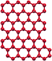
(a)

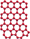
(b)

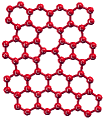
(c)

Figure 1: Schematic representation of hydrogen passivated (a) GQD-64, (b) SW1-GQD-64 and (c) SW2-GQD-64.

III Results and Discussion

In this section, we will first investigate the energy stability, electronic band gaps, and the charge density plots of GQD-64, SW1-GQD-64 and SW2-GQD-64. Thereafter, the conspicuous role played by electron correlation effects in governing the optical properties of these systems are emphasized by a critical analysis of the results obtained from independent particle (TB), PPP model at the restricted Hartree-Fock level (PPP-HF), and the configuration-interaction (CI) methodology (PPP-CI).

III.1 Energy stability, energy band-gap and charge density plots

In Table 1 we report (i) the difference in energy ($\Delta E$) of optimized SW1-GQD-64 and SW2-GQD-64 configurations with respect to pristine GQD-64 (computed from Gaussian 16 program package) and (ii) energy band-gap between the highest occupied (H) and lowest unoccupied (L) molecular orbitals obtained from TB, PPP-HF and the correlated calculations using the PPP-CI approach. A comparison of the energetics of these three systems reveal that GQD-64 has lowest energy followed by SW1-GQD-64 and SW2-GQD-64. This indicates that reconstruction of zigzag to reczag edge (SW1-GQD-64) increases the energy of the system in agreement with earlier theoretical predictions on hydrogen passivated triangular-shaped GQD (Voznyy et al., 2011). Further, quantum dots with reczag edge are more stable as compared to structures having SW defect at the middle (SW2-GQD-64). This implies that the energy stability of GQDs depends crucially on the location of SW defects. At TB and PPP-HF levels, the computed H-L gaps for GQD-64 and SW2-GQD-64 are very close, while the gap is comparatively higher for SW1-GQD-64 configuration. However, on performing the electron-correlated PPP-CI calculations, the gaps for GQD-64 and SW2-GQD-64 increase as compared to their PPP-HF values, while that of SW1-GQD-64 decreases slightly. In addition, these band-gap values are significantly higher than independent particle model results, signifying the importance of electron repulsion effects in these systems. Furthermore, discernible deviation in the gaps calculated at the HF and the CI levels for GQD-64 and SW2-GQD-64, in contrast to their almost identical values for SW1-GQD-64, imply stronger electron-correlation effects in GQD-64 and SW2-GQD-64 as compared to SW1-GQD-64.

Table 1: Energy difference ($\Delta E)$ of SW defected structures with respect to pristine GQD-64 and their HOMO (H)-LUMO (L) band-gap obtained from TB, PPP model at the RHF level and the PPP-CI calculations.

	$\Delta E$	H-L band-gap (eV)
System	(eV)	TB	PPP-HF	PPP-CI
GQD-64	0	0.13	0.74	1.15
SW1-GQD-64	2.77	0.32	0.89	0.87
SW2-GQD-64	4.14	0.14	0.72	1.05

The charge density plots of frontier molecular orbitals contributing significantly to linear absorption spectra computed from TB and PPP model for GQD-64, SW1-GQD-64 and SW2-GQD-64 systems are represented in figs. 2(a-t). In case of GQD-64, the charge density plots of LUMO (L) and L+1 are same as HOMO (H) and H-1 orbitals, respectively, due to the electron-hole symmetry, and hence have not been presented. For GQD-64 (figs. 2(a-d)), the charge is concentrated at the zigzag edges of H (or L) orbital, while for H-1 (or L+1), it is also significant at other atomic sites. In the presence of SW defects (Figs. 2 (e-t)), the electron-hole symmetry is no longer conserved in these orbital pairs. For SW1-GQD-64 (figs. 2(e-l)), the charge distribution is more conspicuous at the zigzag edge for H orbital, while it is more at both the reczag and zigzag edges for L orbital. Further, for H-1 orbital, the charge is quite uniformly distributed over all atomic sites, which is in contrast to the localized nature of charge density near the reczag edge for L+1 orbital. In case of SW2-GQD-64 configuration (figs. 2(m-t)), the charge density is more at the zigzag edge both for H and L orbitals, while at the location of SW defect, it is high for H, H-1 and L+1 orbitals. This charge concentration at the location of SW defects suggests that they will play an important role in determining the electronic band gaps and optical properties of the defective GQDs.

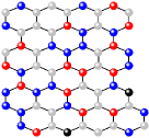
(a)

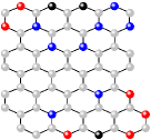
(b)

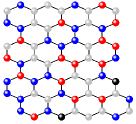
(c)

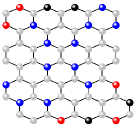
(d)

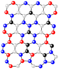
(e)

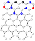
(f)

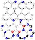
(g)

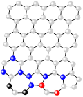
(h)

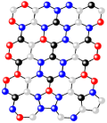
(i)

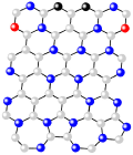
(j)

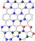
(k)

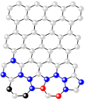
(l)

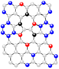
(m)

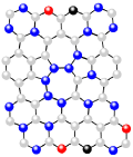
(n)

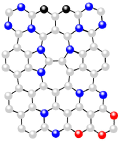
(o)

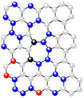
(p)

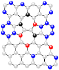
(q)

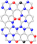
(r)

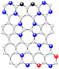
(s)

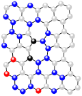
(t)

Figure 2: Charge density plots of H-1, H orbitals of GQD-64 obtained from TB model (a-b) and PPP-HF model (c-d), H-1, H, L, L+1 orbitals of SW1-GQD-64 and SW2-GQD-64 obtained from TB model (e-h and m-p) and PPP-HF model (i-l and q-t). The grey, blue, red and black spheres correspond to $\leq 10\%,$ $>10\%-40\%,$$>40\%-70\%$ and >70% of maximum charge density distribution, respectively.

III.2 Linear absorption spectrum

The significance of electron correlation effects in determining the optical properties of these GQDs are now demonstrated below by critically analyzing the linear absorption spectra computed using the PPP-CI methodology (Figs. 4a, 4b and 4c) with those obtained employing the TB and PPP-HF (Fig. 3) approaches. The reasonably large ($\sim$$10^{6}$) sizes of the CI matrices considered for these GQDs (Table 2) indicate that electron correlation effects are well incorporated in these calculations, thereby signifying the precision of our computations, since no experimental data on optical absorption spectra is available till date on these systems. In addition, detailed quantitative information about the energies, $x$ and $y$ components of the transition dipole moments, and the dominant configurations which contribute to the many particle wave-functions of the excited states primarily responsible for the PPP-CI linear absorption peaks of GQD-64, SW1-GQD-64 and SW2-GQD-64, are listed in tables 3, 4 and 5, respectively.

Table 2: Dimensions of the CI matrices for computing the linear absorption spectra of GQD-64, SW1-GQD-64 and SW2-GQD-64.

System	Dimension of CI Matrix
GQD-64	6118740
SW1-GQD-64	7660787
SW2-GQD-64	8135639

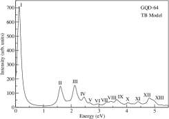
(a)

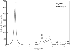
(b)

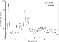
(c)

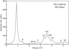
(d)

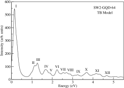
(e)

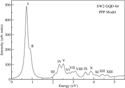
(f)

Figure 3: Linear optical absorption spectra of GQD-64, SW1-GQD-64 and SW2-GQD-64 computed using the tight-binding (TB) model and the PPP model at the HF level. The spectrum has been broadened with a uniform line width of 0.1 eV.

Table 3: Excited states contributing to the linear absorption spectrum of GQD-64, computed using the MRSDCI methodology. Here, $c.c.$ implies the charge-conjugated configuration.

Peak	E (eV)	Transition	Transition	Dominant Configurations
		Dipole (Å) x-component	Dipole (Å) y-component
$I$	$1.15$	$0.70$	$3.31$	$|H\rightarrow L\rangle$$(0.8333)$
				$|H-1\rightarrow L+1\rangle$$(0.1650)$
$II$	$1.90$	$1.30$	$0.27$	$|H\rightarrow L;H\rightarrow L+1\rangle$$+c.c.(0.5665)$
				$|H-3\rightarrow L\rangle$$+c.c.(0.1641)$
$III$	$2.58$	$0.19$	$1.70$	$|H-1\rightarrow L+1\rangle$$(0.4903)$
				$|H-3\rightarrow L\rangle$$+c.c.(0.3696)$
	$2.67$	$0.85$	$1.80$	$|H-1\rightarrow L+1\rangle$$(0.5933)$
				$|H-3\rightarrow L\rangle$$+c.c.(0.3857)$
$IV$	$3.02$	$1.17$	$0.04$	$|H-5\rightarrow L\rangle$$+c.c.(0.3681)$
				$|H-6\rightarrow L\rangle$$-c.c.(0.3513)$
$V$	$3.25$	$0.95$	$1.17$	$|H-5\rightarrow L\rangle$$+c.c.(0.4083)$
				$|H\rightarrow L+6\rangle$$-c.c.(0.3326)$
$VI$	$3.38$	$1.69$	$0.06$	$|H\rightarrow L+7\rangle$$-c.c.(0.5507)$
				$|H\rightarrow L+10\rangle$$+c.c.(0.1321)$
$VII$	$4.25$	$0.22$	$0.11$	$|H\rightarrow L+11\rangle$$-c.c.(0.4248)$
				$|H\rightarrow L;H\rightarrow L+4\rangle$$-c.c.(0.4001)$

Table 4: Excited states contributing to the linear absorption spectrum of SW1-GQD-64, computed employing the MRSDCI methodology.

Peak	E (eV)	Transition	Transition	Dominant Configurations
		Dipole (Å) x-com	Dipole (Å) y-com
$I$	$0.57$	$0.66$	$0.65$	$|H\rightarrow L+1\rangle$$(0.7152)$
				$|H\rightarrow L;H\rightarrow L+1\rangle$$(0.4383)$
$II$	$0.87$	$0.58$	$1.50$	$|H\rightarrow L\rangle$$(0.6061)$
				$|H\rightarrow L;H\rightarrow L\rangle$$(0.3784)$
$III$	$1.42$	$0.22$	$0.96$	$|H\rightarrow L\rangle$$(0.5216)$
				$|H\rightarrow L;H\rightarrow L\rangle$$(0.5072)$
$IV$	$1.65$	$0.11$	$0.45$	$|H-1\rightarrow L\rangle$$(0.5760)$
				$|H\rightarrow L+2\rangle$$(0.3075)$
$V$	$2.06$	$1.11$	$0.60$	$|H\rightarrow L;H\rightarrow L+1\rangle$$(0.4645)$
				$|H\rightarrow L;H-1\rightarrow L\rangle$$(0.4073)$
$VI$	$2.39$	$1.54$	$0.24$	$|H\rightarrow L;H-1\rightarrow L\rangle$$(0.4360)$
				$|H\rightarrow L;H\rightarrow L+2\rangle$$(0.4256)$
$VII$	$2.66$	$0.16$	$0.69$	$|H\rightarrow L+6\rangle$$(0.5775)$
				$|H\rightarrow L+5\rangle$$(0.3303)$
$VIII$	$2.91$	$0.43$	$0.30$	$|H-4\rightarrow L\rangle$$(0.2895)$
				$|H\rightarrow L+6\rangle$$(0.2593)$
				$|H\rightarrow L+4\rangle$$(0.2554)$
				$|H\rightarrow L;H-1\rightarrow L+1\rangle$$(0.2535)$
$IX$	$3.11$	$1.06$	$1.34$	$|H-1\rightarrow L+2\rangle$$(0.5703)$
				$|H-5\rightarrow L\rangle$$(0.4346)$
$X$	$3.38$	$0.66$	$0.48$	$|H\rightarrow L+11\rangle$$(0.4879)$
				$|H-7\rightarrow L\rangle$$(0.3161)$

Table 5: Excited states contributing to the linear absorption spectrum of SW2-GQD-64, computed employing the MRSDCI methodology.

Peak	E (eV)	Transition	Transition	Dominant Configurations
		Dipole (Å) x-com	Dipole (Å) y-com
$I$	$0.65$	$0.97$	$0.51$	$|H-1\rightarrow L\rangle$$(0.7675)$
				$|H\rightarrow L\rangle$$(0.2601)$
$II$	$1.05$	$0.73$	$0.61$	$|H\rightarrow L\rangle$$(0.6223)$
				$|H-1\rightarrow L\rangle$$(0.2684)$
$III$	$1.44$	$0.003$	$0.19$	$|H-1\rightarrow L;H-1\rightarrow L\rangle$$(0.5757)$
				$|H\rightarrow L;H\rightarrow L\rangle$$(0.3828)$
$IV$	$1.86$	$0.92$	$1.41$	$|H-1\rightarrow L+2\rangle$$(0.3857)$
				$|H-1\rightarrow L+1;H\rightarrow L\rangle$$(0.3640)$
				$|H-1\rightarrow L+1\rangle$$(0.3540)$
$V$	$2.07$	$0.33$	$1.53$	$|H-2\rightarrow L\rangle$$(0.5186)$
				$|H\rightarrow L+1;H\rightarrow L\rangle$$(0.3222)$
$VI$	$2.32$	$1.78$	$1.05$	$|H-3\rightarrow L\rangle$$(0.5462)$
				$|H-1\rightarrow L;H-1\rightarrow L+2\rangle$$(0.2991)$
				$|H\rightarrow L+2\rangle$$(0.2941)$
$VII$	$2.85$	$0.88$	$0.60$	$|H-9\rightarrow L\rangle$$(0.3857)$
				$|H-1\rightarrow L+3\rangle$$(0.3838)$
$VIII$	$3.39$	$0.10$	$0.40$	$|H-10\rightarrow L\rangle$$(0.5555)$
				$|H-5\rightarrow L;H\rightarrow L\rangle$$(0.3884)$

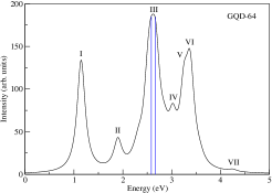
(a)

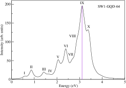
(b)

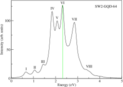
(c)

Figure 4: Linear optical absorption spectra of (a) GQD-64, (b) SW1-GQD-64 and (c) SW2-GQD-64 computed by employing PPP-CI methodology. The spectrum has been broadened with a uniform line width of 0.1 eV. The blue, violet, and the green lines denote the locations of the most intense absorption peaks of these systems.

On examining the calculated spectra of the GQDs and quantitative information about the corresponding excited states (Tables 3-5), we observe the following trends: (i) The first peak of the TB and PPP-HF spectra for all these three systems is due to single excitation of an electron from $H$ to $L$ level, denoted by $|H\rightarrow L\rangle$, corresponding to the optical gap. At the CI level, the excited state wave function of the first peak of GQD-64 corresponding to the optical band-gap (Table 3) is also dominated by the $|H\rightarrow L\rangle$ configuration. On the other hand, the wave functions of the first peaks of SW1-GQD-64 and SW2-GQD-64 are dominated by the transitions $|H\rightarrow L+1\rangle$ and $|H-1\rightarrow L\rangle$, respectively, in contrast to the independent-particle predictions. Further, the configuration $|H\rightarrow L\rangle$ makes major contribution to the wave functions of the excited states giving rise to the second peak of both these SW-defect configurations (Tables 4-5). This implies that in the defective GQDs, the electron correlation effects and the broken particle-hole symmetry due to the presence of SW-type reconstructions, are responsible for the appearance of these first peaks below the ones corresponding to the $|H\rightarrow L\rangle$ dominated second peaks. (ii) At TB and PPP-HF levels, introduction of SW defects at the edge/core of GQD-64 results in marginal blue-shift/no shift of the optical gap, as compared to GQD-64. In contradiction, the PPP-CI calculations predict redshifts in these optical gaps compared to GQD-64, with the decrease being more pronounced for SW1-GQD-64. Further, the entire PPP-CI absorption spectrum of SW2-GQD-64 exhibits a red-shift in comparison to GQD-64, while no such trend is discernable for SW1-GQD-64. (iii) The intensities of the absorption peaks corresponding to the $|H\rightarrow L\rangle$ excitation obtained from TB, PPP-HF and PPP-CI approaches, decrease drastically with the introduction of SW-defects. In addition, the relative strengths of the defect-induced first peaks for SW1-GQD-64/SW2-GQD-64 at the PPP-CI level are always less as compared with the $|H\rightarrow L\rangle$ peaks of the spectra. (iv) The first PPP-CI peaks are not the most intense ones for all the three GQDs, in complete contradiction to the results obtained from the independent particle model, signifying the importance of electron correlation effects. (v) The incorporation of SW-type bond rotations at the edge/middle of the quantum dot leads to a significant blue/red-shift of the maximum intensity (MI) peak in comparison to that of GQD-64 at CI level, which is in contrast to the marginal/no-shift of this peak seen in the TB and PPP-HF results. (vi) The first (I) and sixth (VI) high intensity absorption peaks of pristine GQD-64 are in the infra-red and the UV ranges, respectively, while rest of the strong absorption peaks are in the visible range, resulting in 59% of the total absorption spectrum being in the visible domain. When SW-type bond rotations are present at the edge of GQD-64, all strong absorption peaks except the tenth (X) high intensity peak is in the visible spectrum, increasing the area under visible range to 65%. Also, when SW defects are created at the core of GQD-64, all the high intensity peaks are in the visible range, resulting in 83% of the total CI absorption spectrum being in that domain. These results highlight that the introduction of SW defects in GQD-64 shifts the strong absorption peaks to the visible range, leading to substantial enhancement of visible light absorption. In addition, this improvement in visible light absorption is more pronounced for the SW reconstructions located at the core, as compared to those at the edge of pristine GQD-64. (vii) The strength of the MI peaks computed by the PPP-CI methodology are enhanced/diminished when SW defects are at the edge/centre of the quantum dots, as compared to that of the pristine GQD-64. But, the corresponding peak intensities for the defective GQDs are reduced as compared to GQD-64, when computed using the independent-particle approaches. (viii) The wave functions of the excited states responsible for absorption peaks in GQDs with SW defects demonstrate stronger mixing of several single excitations along with significant contribution from doubly-excited configurations, emphasizing the importance of electron correlation effect in these systems, as compared to pristine GQD-64. (ix) The number of absorption peaks obtained from all the three methodologies increases when SW-type reconstructions are present in the system.

We now provide a detailed discussion of the CI results for the absorption spectra of individual configurations. Figure 4a depicts the computed linear absorption spectrum of GQD-64. The first peak at 1.15 eV (near IR range), corresponding to the optical band-gap, is quite intense and exhibits both x as well as y - polarization. However, the magnitude of transition dipole moment along y-axis is significantly higher than its value along the x-axis. The most intense peak (peak III at energy 2.62 eV) with mixed x-y polarization is due to two closely spaced excited states having energies 2.58 eV and 2.67 eV (blue range of visible spectrum), respectively. The wave-functions of these excited states have dominant contributions from the configurations $|H-1\rightarrow L+1\rangle$ and $|H-3\rightarrow L\rangle+c.c.$, respectively, where c.c. denotes the charge conjugated configuration. The other two high intense peaks (peak V and peak VI) of the absorption spectrum at energies 3.25 eV (violet range of visible spectrum) and 3.38 eV (near UV) are primarily due to single excitations involving higher energy levels $|H-5\rightarrow L\rangle+c.c.$ and $|H\rightarrow L+7\rangle-c.c.$, respectively. Peak V exhibits both x as well as y - polarization while peak VI is dominantly polarized along x-axis. Hence, our results indicate that single excitations are mainly responsible for the appearance of absorption peaks. Further, in contrast to the results obtained from the independent particle model, most of the intense peaks occur at the high energy end of the spectrum, signifying the importance of inclusion of electron correlation effects in predicting the absorption peak profile.

In case of SW1-GQD-64 (fig. 4b), the first weak peak (0.57 eV) with almost equal polarization along both x- and y-axis is primarily due to the single excitation $|H\rightarrow L+1\rangle$, with partial contribution from double excitation $|H\rightarrow L;H\rightarrow L+1\rangle$. The low intensity second peak (0.87 eV) defining the optical band-gap also derives remarkable contribution from the double excitation $|H\rightarrow L;H\rightarrow L\rangle$, and exhibits higher intensities for photons polarized along the $y$-axis, as compared to those polarized along the $x$-axis. The wave-function of the excited state giving rise to the most intense peak (peak IX at 3.11 eV, corresponding to the violet range of the visible spectrum) with mixed $x-y$ polarization is largely composed of the singly excited configurations $|H-1\rightarrow L+2\rangle$ and $|H-5\rightarrow L\rangle$. In addition, the wave-function of the excited state leading to the appearance of high intensity peak VIII at 2.91 eV (violet range), with a mixed $x-y$ character, manifests a strong mixing of singly and doubly excited configurations $|H-4\rightarrow L\rangle$, $|H\rightarrow L+6\rangle$, $|H\rightarrow L+4\rangle$ and $|H\rightarrow L;H-1\rightarrow L+1\rangle$, with almost equal contributions. Similarly, the excited state responsible for the high intensity peak X at energy 3.38 eV (near UV) having mixed $x-y$ polarization is due to single excitations $|H\rightarrow L+11\rangle$ and $|H-7\rightarrow L\rangle$, which involve orbitals far away from the fermi level.

For SW2-GQD-64 (fig. 4c), the first two absorption peaks have very low intensities. The first peak (0.65 eV) with higher magnitude of transition dipole moment along x-axis, as compared to y-axis, is largely composed of single excitation $|H-1\rightarrow L\rangle$, with a weak contribution from $|H\rightarrow L\rangle$. The second peak (1.05 eV) with mixed $x-y$ character is mainly due to the excitation $|H\rightarrow L\rangle$, with some contribution from $|H-1\rightarrow L\rangle$ configuration. The $x-y$ polarized most intense peak VI at 2.32 eV (green spectral line) is mainly due to the single and double excitations $|H-3\rightarrow L\rangle$, $|H\rightarrow L+2\rangle$ and $|H-1\rightarrow L;H-1\rightarrow L+2\rangle$. The high intensity peaks IV (1.86 eV - red spectral line) and VII (2.85 eV - blue spectral line) with mixed $x-y$ character exhibits strong mixing of equally contributing configurations $|H-1\rightarrow L+2\rangle$, $|H-1\rightarrow L+1;H\rightarrow L\rangle$, $|H-1\rightarrow L+1\rangle$ and $|H-9\rightarrow L\rangle$, $|H-1\rightarrow L+3\rangle$, respectively. Furthermore, the excited state giving rise to high intensity peak V at 2.07 eV (orange range of visible spectrum) with larger polarization along y-axis, as compared to x-axis, is mainly composed of the single and double excitations $|H-2\rightarrow L\rangle$ and $|H\rightarrow L+1;H\rightarrow L\rangle$. The contribution of these double excitations in the absorption spectrum is strictly due to the presence of strong electron correlation effects in SW-defected systems.

IV Conclusions

In conclusion, we have performed very large-scale electron-correlated computations employing the PPP Hamiltonian to critically analyze the role played by SW-type bond rotations present at either the zigzag edge, or at the core of GQD-64 in determining its structural, electronic and optical properties. Our computations indicate that SW-type defects increases the energy of pristine GQD-64. In addition, the presence of SW defects at the zigzag edge leads to a lower energy than its location at the middle of the quantum dot. Our electron-correlated results demonstrate that the introduction of SW-type defects is responsible for the appearance of defect-induced peak below the optical band-gap. Also, the variation of the entire absorption peak profile is critically dependent upon the location of SW-type reconstruction. In addition, our studies emphasize that electron correlation effects become more dominant for SW-defected GQDs. Finally, our results signify that the introduction of SW defects in a systematic manner (edge/core of GQD-64) shifts the high intensity edge of optical absorption spectrum to the visible range, leading to significant enhancement of visible light absorption. This mechanism can be efficiently exploited to fabricate novel devices for light harvesting and optoelectronics.

References

- Wang et al. (2016) S. Wang, I. S. Cole, and Q. Li, Chem. Commun. 52, 9208 (2016).
- He et al. (2015) K. He, A. W. Robertson, Y. Fan, C. S. Allen, Y.-C. Lin, K. Suenaga, A. I. Kirkland, and J. H. Warner, ACS Nano 9, 4786 (2015).
- Girit et al. (2009) Ç. Ö. Girit, J. C. Meyer, R. Erni, M. D. Rossell, C. Kisielowski, L. Yang, C.-H. Park, M. F. Crommie, M. L. Cohen, S. G. Louie, and A. Zettl, Science 323, 1705 (2009).
- Chuvilin et al. (2009) A. Chuvilin, J. C. Meyer, G. Algara-Siller, and U. Kaiser, New Journal of Physics 11, 083019 (2009).
- Meyer et al. (2008) J. C. Meyer, C. Kisielowski, R. Erni, M. D. Rossell, M. F. Crommie, and A. Zettl, Nano Letters 8, 3582 (2008).
- Koskinen et al. (2009) P. Koskinen, S. Malola, and H. Häkkinen, Phys. Rev. B 80, 073401 (2009).
- Lee et al. (2010) G.-D. Lee, C. Z. Wang, E. Yoon, N.-M. Hwang, and K. M. Ho, Phys. Rev. B 81, 195419 (2010).
- Koskinen et al. (2008) P. Koskinen, S. Malola, and H. Häkkinen, Phys. Rev. Lett. 101, 115502 (2008).
- Wassmann et al. (2008) T. Wassmann, A. P. Seitsonen, A. M. Saitta, M. Lazzeri, and F. Mauri, Phys. Rev. Lett. 101, 096402 (2008).
- Voznyy et al. (2011) O. Voznyy, A. D. Güçlü, P. Potasz, and P. Hawrylak, Phys. Rev. B 83, 165417 (2011).
- Bhowmick and Waghmare (2010) S. Bhowmick and U. V. Waghmare, Phys. Rev. B 81, 155416 (2010).
- Romanovsky et al. (2012) I. Romanovsky, C. Yannouleas, and U. Landman, Phys. Rev. B 86, 165440 (2012).
- Rodrigues et al. (2011) J. N. B. Rodrigues, P. A. D. Gonçalves, N. F. G. Rodrigues, R. M. Ribeiro, J. M. B. Lopes dos Santos, and N. M. R. Peres, Phys. Rev. B 84, 155435 (2011).
- Ihnatsenka and Kirczenow (2013) S. Ihnatsenka and G. Kirczenow, Phys. Rev. B 88, 125430 (2013).
- Frisch et al. (2016) M. J. Frisch, G. W. Trucks, H. B. Schlegel, G. E. Scuseria, M. A. Robb, J. R. Cheeseman, G. Scalmani, V. Barone, G. A. Petersson, H. Nakatsuji, X. Li, M. Caricato, A. V. Marenich, J. Bloino, B. G. Janesko, R. Gomperts, B. Mennucci, H. P. Hratchian, J. V. Ortiz, A. F. Izmaylov, J. L. Sonnenberg, D. Williams-Young, F. Ding, F. Lipparini, F. Egidi, J. Goings, B. Peng, A. Petrone, T. Henderson, D. Ranasinghe, V. G. Zakrzewski, J. Gao, N. Rega, G. Zheng, W. Liang, M. Hada, M. Ehara, K. Toyota, R. Fukuda, J. Hasegawa, M. Ishida, T. Nakajima, Y. Honda, O. Kitao, H. Nakai, T. Vreven, K. Throssell, J. A. Montgomery, Jr., J. E. Peralta, F. Ogliaro, M. J. Bearpark, J. J. Heyd, E. N. Brothers, K. N. Kudin, V. N. Staroverov, T. A. Keith, R. Kobayashi, J. Normand, K. Raghavachari, A. P. Rendell, J. C. Burant, S. S. Iyengar, J. Tomasi, M. Cossi, J. M. Millam, M. Klene, C. Adamo, R. Cammi, J. W. Ochterski, R. L. Martin, K. Morokuma, O. Farkas, J. B. Foresman, and D. J. Fox, “Gaussian 16 Revision C.01,” (2016), gaussian Inc. Wallingford CT.
- Pople (1953) J. A. Pople, Trans. Faraday Soc. 49, 1375 (1953).
- Pariser and Parr (1953) R. Pariser and R. G. Parr, J. Chem. Phys. 21, 767 (1953).
- Shukla (2002) A. Shukla, Phys. Rev. B 65, 125204 (2002).
- Shukla (2004) A. Shukla, Phys. Rev. B 69, 165218 (2004).
- Basak et al. (2015) T. Basak, H. Chakraborty, and A. Shukla, Phys. Rev. B 92, 205404 (2015).
- Basak and Shukla (2016) T. Basak and A. Shukla, Phys. Rev. B 93, 235432 (2016).
- Basak et al. (2018) T. Basak, T. Basak, and A. Shukla, Phys. Rev. B 98, 035401 (2018).
- Basak and Basak (2020a) T. Basak and T. Basak, Materials Today: Proceedings 26, 2058 (2020a), 10th International Conference of Materials Processing and Characterization.
- Basak and Basak (2020b) T. Basak and T. Basak, Materials Today: Proceedings 26, 2069 (2020b), 10th International Conference of Materials Processing and Characterization.
- Rai et al. (2018) D. K. Rai, H. Chakraborty, and A. Shukla, J. Phys. Chem. C 122, 1309 (2018).
- Ohno (1964) K. Ohno, Theoretica chimica acta 2, 219 (1964).
- Chandross and Mazumdar (1997) M. Chandross and S. Mazumdar, Phys. Rev. B 55, 1497 (1997).
- Sony and Shukla (2010) P. Sony and A. Shukla, Computer Physics Communications 181, 821 (2010).