Emergence of the $\rho$ resonance from the HAL QCD potential in lattice QCD

Abstract

We investigate the $I=1$ $\pi\pi$ interaction using the HAL QCD method in lattice QCD. We employ the (2+1)-flavor gauge configurations on $32^{3}\times 64$ lattice at the lattice spacing $a\approx 0.0907$ fm and $m_{\pi}\approx 411$ MeV, in which the $\rho$ meson appears as a resonance state. We find that all-to-all propagators necessary in this calculation can be obtained with reasonable precision by a combination of three techniques, the one-end trick, the sequential propagator, and the covariant approximation averaging (CAA). The non-local $I=1$ $\pi\pi$ potential is determined at the next-to-next-to-leading order (N²LO) of the derivative expansion for the first time, and the resonance parameters of the $\rho$ meson are extracted. The obtained $\rho$ meson mass is found to be consistent with the value in the literature, while the value of the coupling $g_{\rho\pi\pi}$ turns out to be somewhat larger. The latter observation is most likely attributed to the lack of low-energy information in our lattice setup with the center-of-mass frame. Such a limitation may appear in other P-wave resonant systems and we discuss possible improvement in future. With this caution in mind, we positively conclude that we can reasonably extract the N²LO potential and resonance parameters even in the system requiring the all-to-all propagators in the HAL QCD method, which opens up new possibilities for the study of resonances in lattice QCD.

I Introduction

Understanding the hadronic resonances from the first-principle lattice QCD simulation is one of the most important subjects in particle and nuclear physics. At present, the finite-volume method Luscher (1991); Rummukainen and Gottlieb (1995); Hansen and Sharpe (2012) and the HAL QCD method Ishii et al. (2007); Aoki et al. (2010a); Aoki (2011); Ishii et al. (2012) are employed to extract hadron interactions. The finite-volume method extracts scattering phase shifts through finite-volume energy spectra obtained from temporal correlation functions. It has been successfully applied for various two-meson interactions and related mesonic resonances Briceno et al. (2018). In particular, the $\rho$ resonance has been studied extensively Aoki et al. (2011a); Feng et al. (2011); Lang et al. (2011); Dudek et al. (2013); Wilson et al. (2015); Alexandrou et al. (2017); Andersen et al. (2019); Werner et al. (2020); Fischer et al. (2020) as a benchmark, since it is experimentally well-established and is easily investigated by the single-channel approximation of the $I=1$ $\pi\pi$ P-wave scattering. Recent studies report the results with multiple lattice spacings Werner et al. (2020), and those with pion masses including physical masses Fischer et al. (2020).

The HAL QCD method directly constructs inter-hadron potentials from spatial and temporal correlation functions calculated in lattice QCD. In this method, the potentials can be extracted even without ground state saturations for correlation functions Ishii et al. (2012). Scattering parameters are then obtained by solving the Schrödinger equation in infinite-volume without any model-dependent ansatz. These features make this method particularly useful to study baryonic systems Iritani et al. (2019a) and coupled channel systems Aoki et al. (2011b). The HAL QCD method has been successfully applied to many hadronic systems (see Ref. Aoki and Doi (2020) and references therein for the recent status), including the detailed coupled channel studies for the tetraquark candidate $Z_{c}(3900)$ Ikeda et al. (2016); Ikeda (2018) and $H$-dibaryon Sasaki et al. (2020).

There exists, however, a practical challenge in the HAL QCD method when expanding the scope to many other resonances, since the expensive computations of all-to-all quark propagators are necessary in most cases. To overcome this difficulty, we have previously explored two different all-to-all techniques, the LapH methodPeardon et al. (2009) and the hybrid methodFoley et al. (2005). It turned out Kawai et al. (2018); Kawai (2018) that the LapH smearing on sink operators with a small number of LapH vectors enhances non-locality of the HAL QCD potential and thus the systematic errors associated with the truncation of the derivative expansion. Increasing the number of LapH vectors to minimize such non-locality is practically impossible for larger volumes. On the other hand, the hybrid method with local sink operators is free from the enhancement of the non-locality and is more suitable for the HAL QCD method. A series of studies with the hybrid method Akahoshi et al. (2019, 2020), however, has revealed that it requires too much numerical cost for a reduction of stochastic noises to perform large-scale simulations for hadronic resonances.

In this paper, we develop a new strategy to handle all-to-all propagators, where we combine three techniques in lattice QCD, the one-end trickMcNeile and Michael (2006), the sequential propagator calculationMartinelli and Sachrajda (1989) and the covariant approximation averaging (CAA)Shintani et al. (2015). We calculate the HAL QCD potential of the $I=1$ $\pi\pi$ scattering on gauge configurations at $m_{\pi}\approx 411$ MeV, where the $\rho$ meson is known to appear as a resonance with $m_{\rho}\approx 892$ MeVAoki et al. (2011a). Numerical accuracy in our new strategy allows us to determine the non-local $I=1$ $\pi\pi$ potential at the next-to-next-to-leading order (N²LO) in the derivative expansion for the first time. Accordingly, resonance parameters are extracted also by the N²LO analysis. A resonance mass of the $\rho$ meson is found to be consistent with previous studies, while a somewhat larger value of the $\rho\pi\pi$ coupling is obtained. The latter discrepancy is most likely attributed to the lack of low-energy information in our lattice setup with the center-of-mass frame, indicating that calculations with the laboratory frameAoki (2020) in addition to the center-of-mass frame are desirable to study generic P-wave systems in future.

This paper is organized as follows. In Sect. II, we briefly introduce the HAL QCD method and explain correlation functions relevant to our calculation. Sect. III summarizes simulation details. In Sect. IV, we first present results from the leading order (LO) analysis for two different source operators. Then, as our main results, we give the N²LO order potential and resonance parameters, which are compared with the previous results in the finite-volume method. Sect. V is devoted to a summary of this study. In Appendix A, we explain the one-end trick, which is a clever way to treat a certain combination of all-to-all propagators. Details of calculations of quark contraction diagrams are given in Appendix B, while possible effects of smeared quarks for sink operators are investigated in Appendix C. Some details on the N²LO analysis, namely the assumption in the potential fit and behavior of our N²LO potential in terms of energy-dependent local manner, are given in Appendix D and E.

II The HAL QCD method

A fundamental quantity in the HAL QCD method is the Nambu-Bethe-Salpeter (NBS) wave function, which is defined as

$$\psi_{W}({\bf r})=\langle 0|(\pi\pi)_{I=1,I_{z}=0}({\bf r},0)|\pi\pi;I=1,I_{z}=0,{\bf k}\rangle,$$ (1)

where $|\pi\pi;I=1,I_{z}=0,{\bf k}\rangle$ is an asymptotic state for an elastic $I=1$ $\pi\pi$ system in the center-of-mass frame with a relative momentum ${\bf k}$, a total energy $W=2\sqrt{m_{\pi}^{2}+k^{2}}$ and $k=|{\bf k}|$. The operator $(\pi\pi)_{I=1,I_{z}=0}({\bf r},t)$ is a two-pion operator projected to the $I=1,I_{z}=0$ channel given by

$$(\pi\pi)_{I=1,I_{z}=0}({\bf r},t) = \frac{1}{\sqrt{2}}\{\pi_{s}^{+}({\bf r+x},t)\pi_{s}^{-}({\bf x},t)-\pi_{s}^{-}({\bf r+x},t)\pi_{s}^{+}({\bf x},t)\},$$ (2)

$$\pi_{s}^{+}({\bf x},t) = \bar{d}_{s}({\bf x},t)\gamma_{5}u_{s}({\bf x},t),\quad\pi_{s}^{-}({\bf x},t)=\bar{u}_{s}({\bf x},t)\gamma_{5}d_{s}({\bf x},t),$$ (3)

where $u_{s},d_{s}$ are smeared up and down quark fields. A detail of the quark smearing is given in Sect. III. A radial part of the $l$-th partial component in the NBS wave function behaves at large $r=|{\bf r}|$ as Aoki et al. (2010a, 2013a)

$$\psi^{l}_{W}(r)\approx A_{l}({\bf k})e^{i\delta_{l}(k)}\frac{\sin(kr-l\pi/2+\delta_{l}(k))}{kr},$$ (4)

where $A_{l}({\bf k})$ is an overall factor and $\delta_{l}(k)$ is a scattering phase shift, which is equal to a phase of the S-matrix implied by its unitarity. By using this property, we can construct an energy-independent non-local potential $U({\bf r},{\bf r^{\prime}})$ as

$$\frac{1}{2\mu}(\nabla^{2}+k^{2})\psi_{W}({\bf r})=\int d^{3}{\bf r^{\prime}}\,U({\bf r},{\bf r^{\prime}})\psi_{W}({\bf r^{\prime}}),$$ (5)

with $\mu=m_{\pi}/2$ a reduced mass of two pions. In general, the HAL QCD potential depends on a choice of hadron operators in the NBS wave function (the sink operator $(\pi\pi)_{I=1,I_{z}=0}({\bf r},t)$ in our case), and it is referred to as the scheme dependence of the potential Aoki et al. (2012a); Kawai et al. (2018). Physical observables extracted from potentials in different schemes, of course, agree with each other by construction. Therefore, we can utilize this scheme dependence to reduce statistical and/or systematic uncertainties of observables. As discussed in Appendix C, a comparison of different schemes shows that the $I=1$ $\pi\pi$ potential has much smoother ${\bf r}$ dependences in an “equal-time smeared-sink scheme” (Eq.(2)), where sink quark fields are slightly smeared and two pion operators are put on the same time slice. We employ this scheme for the whole analysis in this study.

To extract the potential in lattice QCD simulations, we begin with a normalized correlation function defined as

$$R({\bf r},t)\equiv\frac{F_{\pi\pi}({\bf r},t)}{F_{\pi}(t)^{2}},$$ (6)

where $F_{\pi}$ and $F_{\pi\pi}$ are a single-pion and a two-pion correlation function, respectively,

$$F_{\pi}(t) = \sum_{{\bf x,y},t_{0}}\langle\pi^{-}({\bf x},t+t_{0})\pi^{+}({\bf y},t_{0})\rangle,$$ (7)

$$F_{\pi\pi}({\bf r},t) = \sum_{t_{0}}\langle(\pi\pi)_{I=1,I_{z}=0}({\bf r},t+t_{0})\overline{{\mathcal{J}}}^{T_{1}^{-}}_{I=1,I_{z}=0}(t_{0})\rangle.$$ (8)

Here $\overline{{\mathcal{J}}}^{T_{1}^{-}}_{I=1,I_{z}=0}(t_{0})$ is a source operator which creates $\pi\pi$ scattering states with $(I,I_{z})=(1,0)$ in an irreducible representation $T_{1}^{-}$ of the cubic group. Thus $R({\bf r},t)$ is related to the NBS wave function as

$$R({\bf r},t)=\sum_{n}{B_{n}}\psi_{W_{n}}({\bf r})e^{-(W_{n}-2m_{\pi})t}+\cdots,$$ (9)

where $W_{n}$ and $B_{n}$ are energy and overlap factor of the $n$-th elastic state, and the ellipses indicate inelastic contributions. Using the energy independence of the potential, we can show thatIshii et al. (2012)

$$\left[\frac{\nabla^{2}}{2\mu}-\frac{\partial}{\partial t}+\frac{1}{8\mu}\frac{\partial^{2}}{\partial t^{2}}\right]R({\bf r},t)=\int d^{3}{\bf r^{\prime}}U({\bf r},{\bf r^{\prime}})R({\bf r^{\prime}},t),$$ (10)

at a sufficiently large $t$ where inelastic contributions in $R({\bf r},t)$ becomes negligible. In actual calculations, we introduce a derivative expansion to treat the non-local potential as

$$U({\bf r},{\bf r^{\prime}})=(V_{0}(r)+V_{2}(r)\nabla^{2}+{\mathcal{O}}(\nabla^{4}))\delta({\bf r-r^{\prime}}),$$ (11)

and the effective LO potential is given by

$$V^{\rm LO}(r)=\frac{\sum_{g\in O_{h}}R^{{\dagger}}(g{\bf r},t)\left[\dfrac{\nabla^{2}}{2\mu}-\dfrac{\partial}{\partial t}+\dfrac{1}{8\mu}\dfrac{\partial^{2}}{\partial t^{2}}\right]R(g{\bf r},t)}{\sum_{g\in O_{h}}R^{{\dagger}}(g{\bf r},t)R(g{\bf r},t)},$$ (12)

where invariance of the potential under the cubic rotation group $O_{h}$ is utilized to improve signals Murano et al. (2014). In this study, we further determine the effective N²LO potential in order to extract resonance parameters more accurately. The effective N²LO potential $U^{\rm N^{2}LO}({\bf r},{\bf r^{\prime}})=\left(V_{0}^{\rm N^{2}LO}+V_{2}^{\rm N^{2}LO}\nabla^{2}\right)\delta({\bf r}-{\bf r^{\prime}})$ is determined by solving the following linear equations Iritani et al. (2019b):

$$\left(\begin{array}[]{cc}1&\nabla^{2}R_{A}({\bf r},t)/R_{A}({\bf r},t)\\ 1&\nabla^{2}R_{B}({\bf r},t)/R_{B}({\bf r},t)\end{array}\right)\left(\begin{array}[]{c}V^{\rm N^{2}LO}_{0}(r)\\ V^{\rm N^{2}LO}_{2}(r)\end{array}\right)=\left(\begin{array}[]{c}V^{\rm LO}_{A}(r)\\ V^{\rm LO}_{B}(r)\end{array}\right),$$ (13)

where $R_{i}\ (i=A,B)$ are the normalized correlation functions with different source operators $\overline{{\mathcal{J}}}_{i}(t_{0})\ (i=A,B)$, and $V^{\rm LO}_{i}(r)\ (i=A,B)$ are the effective LO potentials obtained by $R_{i}\ (i=A,B)$. Note that coefficients $V_{0}(r),V_{2}(r)$ in the full derivative expansion (Eq.(11)) are independent of source operators, while effective N²LO coefficients $V_{0}^{\rm N^{2}LO}(r),V_{2}^{\rm N^{2}LO}(r)$ depend on a choice of source operators. In other words, effective potentials implicitly depend on discrete energy levels included in their determination due to the truncation of the derivative expansion Aoki and Doi (2020). Therefore, systematic errors in the derivative expansion for physical observables depend on the magnitude of non-locality in the true potential as well as on the difference between the energy region relevant for physical observables and that employed to determine the effective potentials Aoki and Doi (2020).

For the source operators, we choose $\rho$-type $\overline{{\mathcal{J}}}^{T_{1}^{-}}_{\rho,I=1,I_{z}=0}(t_{0})$ and $\pi\pi$-type $\overline{{\mathcal{J}}}^{T_{1}^{-}}_{\pi\pi,I=1,I_{z}=0}(t_{0})$ in this study, defined by

$$\overline{{\mathcal{J}}}^{T_{1}^{-}}_{\rho,I=1,I_{z}=0}(t_{0}) = \overline{\rho}^{0}_{3}(t_{0}),$$ (14)

$$\overline{{\mathcal{J}}}^{T_{1}^{-}}_{\pi\pi,I=1,I_{z}=0}(t_{0}) = \overline{(\pi\pi)}_{I=1,I_{z}=0}({\bf p}_{3},t_{0}),$$ (15)

where ${\bf p}_{3}=(0,0,2\pi/L)$. $\overline{(\pi\pi)}_{I=1,I_{z}=0}({\bf p},t)$ and $\overline{\rho}^{0}_{3}$ are given as

$$\overline{\rho}^{0}_{3}(t) = \sum_{{\bf x}}\frac{1}{\sqrt{2}}\left(\bar{u}({\bf x},t)\gamma_{3}u({\bf x},t)-\bar{d}({\bf x},t)\gamma_{3}d({\bf x},t)\right)$$ (16)

$$\overline{(\pi\pi)}_{I=1,I_{z}=0}({\bf p},t) = \frac{1}{\sqrt{2}}\sum_{{\bf y_{1},y_{2}}}e^{-i{\bf p\cdot y_{1}}}e^{i{\bf p\cdot y_{2}}}\left(\pi^{-}({\bf y_{1}},t)\pi^{+}({\bf y_{2}},t)-\pi^{+}({\bf y_{1}},t)\pi^{-}({\bf y_{2}},t)\right),$$ (17)

where we use local quark fields for source operators.

Calculations of correlation functions with momentum projected sources generally need all-to-all propagators, which requires too much numerical cost to calculate exactly. Therefore, we evaluate all-to-all propagators by the combination of the one-end trick, the sequential propagator, and the CAA. We give a brief introduction of the one-end trick in Appendix A, and details of diagram calculations are presented in Appendix B.

III Simulation details

We employ (2+1)-flavor full QCD configurations generated by the PACS-CS Collaborations Aoki et al. (2009) on a $32^{3}\times 64$ lattice with the Iwasaki gauge actionIwasaki (1985) at $\beta=1.90$ and a non-perturbatively improved Wilson-clover actionSheikholeslami and Wohlert (1985) at $c_{SW}=1.715$ and hopping parameters $(\kappa_{ud},\kappa_{s})=(0.13754,0.13640)$. These parameters correspond to a lattice spacing $a=0.0907$ fm, and a pion mass $m_{\pi}\approx 411$ MeV, where the $\rho$ meson appears as a resonance with $m_{\rho}\approx 892$ MeV Aoki et al. (2011a). The calculations are performed in the center-of-mass frame with the periodic boundary condition for all spacetime directions. In this report, dimensionful quantities without the corresponding unit are written in lattice unit unless otherwise stated.

Table 1: Numerical setup for the calculation.

Source type	Scheme	$N_{\rm conf}$ (#. of time slice ave.)	Stat. error
$\pi\pi$-type	equal-time, smeared-sink	100 (64)	jackknife with bin–size 5
$\rho$-type	equal-time, smeared-sink	200 (64)	jackknife with bin–size 10

Table 2: Setups for the one-end trick and the CAA in this study. $N_{\rm eig}$ is the number of low eigenmodes. Color and spinor dilutions are always used.

Source type	One-end trick		CAA
	Noise vector	Space dilution	$N_{\rm eig}$	# of averaged points
$\pi\pi$-type	$Z_{4}$ noise	$s2$ (even-odd)	300	64
$\rho$-type	$Z_{4}$ noise	$s4$	300	64

Table 1 and 2 show general setups and parameters of the one-end trick and the CAA, respectively. We employ smeared quark operators $q_{s}({\bf x},t)=\sum_{\bf y}f({\bf x-y})q({\bf y},t)$ at the sink with the Coulomb gauge fixing, in order to improve signals of potentials at short distance. A smearing function $f$ is given by

$$f\left({\bf x}\right)=\begin{cases}Ae^{-B|{\bf x}|}&(\ 0<|{\bf x}|<R\ )\\ 1&(\ |{\bf x}|=0\ )\\ 0&(\ |{\bf x}|\geq R\ ),\end{cases}$$ (18)

with $A=1.0,\ B=1.0,\ R=3.5$. As discussed in Appendix C, these parameters make potential smoother without worsening the convergence of the derivative expansion. For the one-end trick, we generate a single $Z_{4}$ noise vector for each insertion. To suppress the corresponding stochastic noises, we employ a dilution technique Foley et al. (2005) in color, spinor and space indices. Color and spinor indices are fully diluted, and for the space dilution, we take $s2$ (even-odd) dilution and $s4$ dilution Akahoshi et al. (2020) in the $\pi\pi$-type source and the $\rho$-type source, respectively. In the CAA, we exactly estimate a low-mode part with 300 eigenmodes, and a high-mode part is estimated by an average over loosely solved solutions on 64 different spatial points ${\bf x}=(x_{0}+8l,y_{0}+8m,z_{0}+8n)\ {\rm mod}\ 32$, with $l,n,m\in\{0,1,2,3\}$. Finer and looser solutions are obtained with $1.0\times 10^{-24}$ and $9.0\times 10^{-9}$ for the squared residue, respectively. We randomly choose the reference point ${\bf x}_{0}=(x_{0},y_{0},z_{0})$ for each configuration.

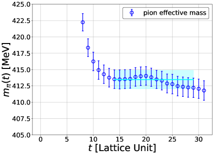
Figure 1: Effective mass of a pion (blue circles) and the fit result by a cosh function at $t=[t_{\rm min},t_{\rm max}]=[14,29]$ (cyan solid line with bands).

Figure 1 (left) show an effective mass of a pion obtained by an average over 200 configurations ($\times 64$ time slice average). A fit to the pion propagator $F_{\pi}(t)$ at $t=[t_{\rm min},t_{\rm max}]=[14,29]$ with a cosh function gives $m_{\pi}=413.5(1.4)$ MeV. We also check a $t_{\rm min}$ dependence of the effective mass, and the dependence is negligible compared with statistical errors as far as $t_{\rm min}\geq 13$. Therefore we confirm that a ground state saturation in $F_{\pi}(t)$ is achieved at $t=13$. A possible leading inelastic contribution for two pions in this setup comes from a P-wave $K\overline{K}$ state with energy $W_{K\overline{K}}=2\sqrt{m_{K}^{2}+(2\pi/L)^{2}}\approx 1530$ MeV in non-interacting case, while the two-pion ground state energy is reported as $E_{0}=914(11)$ MeV in Ref. Aoki et al. (2011a). We therefore expect inelastic contributions in $F_{\pi\pi}({\bf r},t)$ are suppressed at $t\approx 1/[W_{K\overline{K}}-E_{0}]\approx 3.5$. These considerations suggest that inelastic contributions in $R({\bf r},t)$ become negligible at $t\geq 13$, so that potentials can be reliably extracted at $t\geq 13$. Hereafter, we show results at $t=14$ and $18$ for $\rho$-type source and $\pi\pi$-type source, respectively.

In lattice QCD, the rotational symmetry is broken to the cubic symmetry, and there exist higher partial wave components in the irreducible representation of the cubic group ($l=3,5,\cdots$ partial waves in this study). This leads to systematic uncertainties in the HAL QCD potential, which exhibit as multi-valued structures of potentials as a function of $r$. We address this issue by performing the approximated partial wave decomposition recently introduced to lattice QCD Miyamoto et al. (2020). In practice, we remove the dominant contaminations, the $l=3$ partial wave component, when we evaluate the potential at $r=[2,14.8]$. Tunable parameters of the decomposition Miyamoto et al. (2020), a number of radial bases $n_{\rm max}$, a number of partial waves considered $l_{\rm max}$ and a width of the shell $\Delta$, are taken as $(n_{\rm max},l_{\rm max},\Delta)=(4,5,1.2)$ at $2\leq r\leq 10$ or $(4,5,1.5)$ at $r>10$, where we use larger $\Delta$ at larger $r$ to avoid artificial oscillation of decomposed data due to too small $\Delta$.

IV Result

IV.1 Effective leading-order potentials

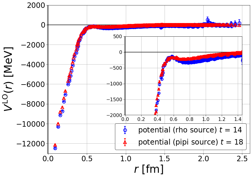
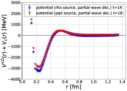
Figure 2: (Left) Effective LO potentials. Blue and red points show the results from the $\rho$-type source and the $\pi\pi$-type source, respectively. Inset shows an enlarged view of potentials. (Right) Improved potentials obtained by the partial wave decomposition with the P-wave centrifugal term, $V_{c}(r)=\frac{1}{2\mu}\frac{1\cdot 2}{r^{2}}$.

Figure 2 (Left) show the results for effective LO potentials without the partial wave decomposition. We observed that the potentials are attractive at all distances. Fig. 2 (Right) represents potentials after the partial wave decomposition with the P-wave centrifugal term added, which become much smoother as multi-valued structures are eliminated. The potentials with the centrifugal term reveal characteristic features for an existence of a resonance state such as an attractive pocket at short distances and a potential barrier around $r=0.5$ fm. We also notice that potentials obtained from different source operators are different from each other, which fact suggests a presence of non-negligible higher-order contributions in the derivative expansion.

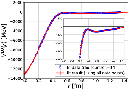
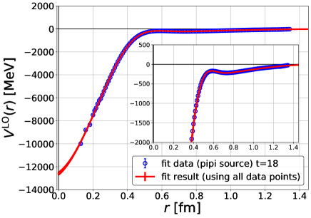
Figure 3: (Left) Fit result with the $\rho$-type source. Inset shows an enlarged view of them. (Right) The same plot with the $\pi\pi$-type source. Both results are obtained with all allowed data points.

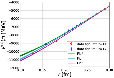
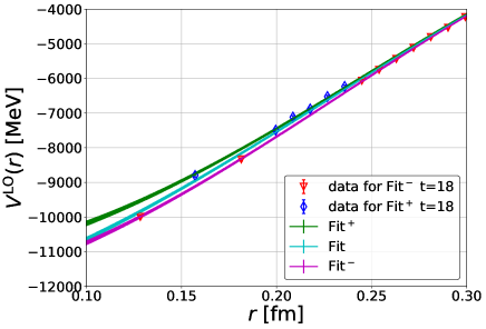
Figure 4: Systematic uncertainty in the fit of the potential at short distances. (Left) Three fit results with the $\rho$-type source. Red and blue points show data used in Fit^- and Fit⁺, respectively, and magenta and green lines are results of Fit^- and Fit⁺. We also show the fit result with all allowed data (Fit) by a cyan line for a comparison. (Right) The same plot with the $\pi\pi$-type source.

Table 3: Fit parameters for effective LO potential with the $\pi\pi$-type source.

	$a_{0}$	$a_{1}$	$a_{2}$	$a_{3}$	$a_{4}$	$a_{5}$	$a_{6}$	$a_{7}$	$a_{8}$	$\chi^{2}/{\rm dof.}$
Fit	-0.0821(42)	8.04(38)	5.15(44)	-5.94(11)	-0.649(93)	3.995(74)	0.548(21)	4.670(15)	2.009(26)	0.85
Fit+	-0.0976(75)	6.95(63)	5.75(56)	-5.20(10)	-0.09(10)	3.658(99)	0.525(34)	4.611(17)	2.0286(34)	0.24
Fit-	-0.0983(10)	6.84(79)	5.84(57)	-5.66(14)	-0.28(14)	3.76(17)	0.574(71)	4.517(43)	2.109(53)	0.14

Table 4: Fit parameters for effective LO potential with the $\rho$-type source.

	$a_{0}$	$a_{1}$	$a_{2}$	$a_{3}$	$a_{4}$	$a_{5}$	$a_{6}$	$a_{7}$	$a_{8}$	$\chi^{2}/{\rm dof.}$
Fit	-0.1146(74)	9.64(33)	5.23(47)	-6.35(17)	-1.03(15)	4.456(95)	0.711(25)	4.818(23)	2.068(29)	1.15
Fit+	-0.124(11)	8.89(65)	5.83(68)	-5.57(16)	-0.42(15)	4.12(14)	0.712(41)	4.752(27)	2.111(36)	0.29
Fit-	-0.120(17)	9.1(1.1)	5.75(97)	-6.18(21)	-0.74(23)	4.34(27)	0.81(11)	4.650(72)	2.227(79)	0.18

We fit LO potentials with a sum of Gaussian terms given by

$$V(r)=a_{0}e^{-(r-a_{1})^{2}/a_{2}^{2}}+a_{3}e^{-(r-a_{4})^{2}/a_{5}^{2}}+a_{6}e^{-(r-a_{7})^{2}/a_{8}^{2}}.$$ (19)

For the fit, we utilize data projected to the $l=1$ component by the partial wave decomposition at $r=[2,14.8]$ as already discussed, combined with the original lattice data at $r\leq 2$, to which the partial wave decomposition cannot be reliably applied. We also remove data at very short distances ($r=0,1$) since they suffer from large discretization errors. Remaining systematic uncertainties caused by non-smoothness at short distances are estimated by differences among three different fit results: a result using all allowed data (Fit), a result removing data at $r\leq 0.32$ fm which are significantly larger than Fit (Fit^-), and a result removing data at $r\leq 0.32$ fm which are significantly smaller than Fit (Fit⁺). The fit results using all allowed data (Fit) are shown in Figure 3, and comparisons of three fit results at short distances are given in Figure 4. Resultant fit parameters and $\chi^{2}/{\rm dof}$ are given in Table. 3 and 4. As seen in Fig.4, the non-smooth behavior of the potential at short distances, which is probably caused by contaminations from higher partial waves, affects the fit result at $r\lesssim 0.25$ fm. Since the removal of such contaminations at short distances is impractical, we estimate systematic errors for physical observables by differences among fit results, taking the result using all allowed data as a central value.

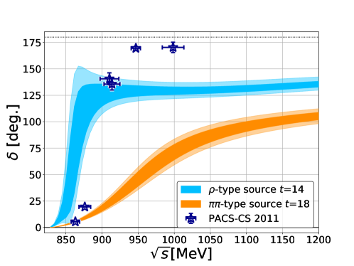
Figure 5: Phase shifts at the LO analysis. Blue (orange) band shows the $\rho$-type ($\pi\pi$-type) source result. Statistical errors are given by dark color bands, whereas systematic errors estimated by three different fits at short distances are represented by light color bands. The previous finite-volume results by the PACS-CS Collaboration Aoki et al. (2011a) are also given by navy stars for comparison.

Figure 5 shows phase shifts obtained from fitted potentials, where systematic errors associated with removals of data at short distances are shown by light color bands on top of statistical errors by dark color bands. Shown together is the previous finite-volume result reported in Ref. Aoki et al. (2011a), which employs the same gauge configurations. The phase shift obtained with the $\rho$-type source crosses 90 degrees around $\sqrt{s}\approx 870$ MeV, while it only reaches around 130 degrees as the energy increases. On the other hand, the phase shift obtained with the $\pi\pi$-type source crosses 90 degrees at much higher energy, around $\sqrt{s}\approx 1050$ MeV, with much broader width. These behaviors are probably caused by truncation errors of the derivative expansion for the LO potential. Since the $\rho$-type source strongly overlaps the $\rho$ resonance state, which corresponds to the ground state in this setup, the resultant phase shift with the $\rho$ source reproduces the $\rho$ resonance structure relatively well. On the other hand, since the $\pi\pi$-type source mainly overlaps P-wave $\pi\pi$ scattering states, which appear in the energy region far above the $\rho$ resonance in this lattice setup, it is difficult for the phase shift with the $\pi\pi$-type source to capture the resonance structure correctly.

IV.2 The N²LO analysis

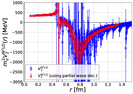
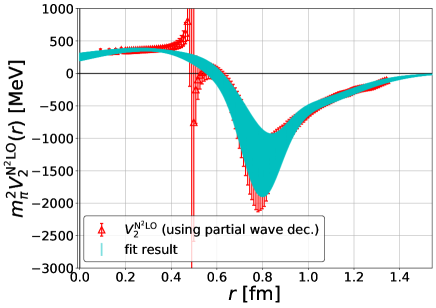
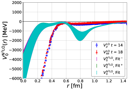
Figure 6: Effective N²LO potentials. (Upper left) $V_{2}^{\rm N^{2}LO}$ determined from raw data (blue circles) and data obtained with the partial wave decomposition (red triangles). (Upper right) The fit result (cyan band) using the decomposed data (red triangles). (Lower) $V_{0}^{\rm N^{2}LO}$ obtained by three fit results , Fit(cyan), Fit^-(magenta) and Fit⁺(green). Shown together are the effective LO potentials for a comparison.

As we have two LO potentials, we can proceed to the N²LO analysis. The effective N²LO potentials are obtained through eq.(13) as

$$V_{2}^{\rm N^{2}LO}(r) = \frac{V_{\rho}^{\rm LO}(r)-V_{\pi\pi}^{\rm LO}(r)}{\nabla^{2}R_{\rho}(r)/R_{\rho}(r)-\nabla^{2}R_{\pi\pi}(r)/R_{\pi\pi}(r)}$$ (20)

$$V_{0}^{\rm N^{2}LO}(r) = V_{\rho}^{\rm LO}(r)-V_{2}^{\rm N^{2}LO}(r)\nabla^{2}R_{\rho}(r)/R_{\rho}(r).$$ (21)

In Fig. 6 (upper left), we show $V_{2}^{\rm N^{2}LO}$ obtained from raw data (blue points), and $l=1$ data with the partial wave decomposition (red points). Thanks to the removal of higher partial wave contaminations, we can significantly reduce fluctuations of $V_{2}^{\rm N^{2}LO}$, as seen in the figure.

A somewhat singular behavior at $r\approx 0.5$ fm is caused by a vanishing denominator of $V_{2}^{\rm N^{2}LO}$ in Eq.(20). We however expect that this singular behavior is canceled by a vanishing numerator at the same point. As discussed in Appendix D, this expectation is shown to be true as long as the N⁴LO (and higher order) terms in the derivative expansion are negligible. Furthermore, we assume that $1-2\mu V_{2}^{\rm N^{2}LO}>0$, which is also shown to be true in Appendix D if the N⁴LO or higher order terms are negligible. We thus fit $V_{2}^{\rm N^{2}LO}$ (red point) by a smooth function, a 3-Gaussian function in Eq (19), where data with $1-2\mu V_{2}^{\rm N^{2}LO}\leq 0$ are excluded in the fit. Fit parameters for $V_{2}^{\rm N^{2}LO}$ are summarized in Table 5 and the fit result is shown by a cyan band in Fig. 6 (upper right). Since significant non-smooth behavior is not observed for $V_{2}^{\rm N^{2}LO}$ at short distances, systematic errors associated with removals of data mentioned before are not included in the analysis for $V_{2}^{\rm N^{2}LO}$.

Table 5: Fit parameters of the $V_{2}^{\rm N^{2}LO}$.

$a_{0}$	$a_{1}$	$a_{2}$	$a_{3}$	$a_{4}$	$a_{5}$	$a_{6}$	$a_{7}$	$a_{8}$	$\chi^{2}/dof$
-12.8(6.4)	8.82(24)	1.37(11)	-9.4(5.8)	9.86(94)	3.97(78)	5.7(4.7)	4.8(2.4)	6.48(72)	0.063

Table 6: Fit parameters of the Laplacian term $\nabla^{2}R_{\rho}/R_{\rho}$.

	$a_{0}$	$a_{1}$	$a_{2}$	$a_{3}$	$a_{4}$	$a_{5}$	$a_{6}$	$a_{7}$	$a_{8}$	$\chi^{2}/dof$
Fit	-0.0271(12)	9.04(43)	6.21(36)	-1.135(25)	-0.70(13)	4.33(12)	0.1452(78)	4.743(26)	2.143(36)	3.44
Fit+	-0.0270(18)	9.03(67)	6.25(52)	-0.993(19)	-0.07(11)	4.17(14)	0.175(18)	4.591(46)	2.264(61)	1.54
Fit-	-0.0249(16)	9.71(61)	5.76(50)	-1.165(24)	-0.71(15)	4.56(15)	0.188(20)	4.550(60)	2.348(69)	1.09

Let us consider a determination of $V_{0}^{\rm N^{2}LO}(r)$ next. We first fit the Laplacian term $\nabla^{2}R_{\rho}(r)/R_{\rho}(r)$ by the same 3-Gaussian function, and resultant parameters are given in Table 6. We then obtain $V_{0}^{\rm N^{2}LO}(r)$ by combining all the fit results in Eq. (21). We estimate systematic errors of $V_{0}^{\rm N^{2}LO}(r)$ at short distances through those of $V_{\rho}^{\rm LO}$ and $\nabla^{2}R_{\rho}(r)/R_{\rho}(r)$. Figure 6(lower) shows the resultant $V_{0}^{\rm N^{2}LO}$, together with effective LO potentials, $V_{\rho}^{\rm LO}$ and $V_{\pi\pi}^{\rm LO}$, for a comparison. As expected, there exists a large difference between $V_{\rho,\pi\pi}^{\rm LO}$ and $V_{0}^{\rm N^{2}LO}$ in Fig. 6 (lower).

To obtain the N²LO phase shifts, we solve the radial Schrödinger equation with the N²LO potential, rewritten as

$$\left(\frac{d^{2}}{dr^{2}}-\frac{l(l+1)}{r^{2}}-\frac{2\mu V_{0}(r)-k^{2}}{1-2\mu V_{2}(r)}\right)\phi=0.$$ (22)

The N²LO phase shifts and the corresponding $k^{3}\cot\delta_{1}/\sqrt{s}$ are shown in Figure 7, together with the LO phase shifts and the previous finite-volume result for comparisons. We have checked that the N²LO phase shifts do not vary beyond the magnitude of statistical errors even if we choose a different timeslice for the $\pi\pi$-type source in the N²LO analysis.

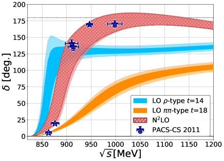
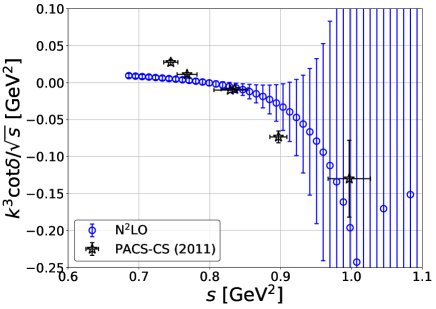
Figure 7: The N²LO phase shifts (left) and $k^{3}\cot\delta_{1}/\sqrt{s}$ (right), together with LO results (left figure) and previous finite-volume result by the PACS-CS Collaboration Aoki et al. (2011a) (both figure) for comparisons. Large statistical errors at $s>0.9$ GeV² in $k^{3}\cot\delta_{1}/\sqrt{s}$ (right) are mainly caused by a divergent behavior of $\cot\delta$ at the phase shift around 180 degrees.

As can be seen in Fig. 7, except for the region $s<0.75\ {\rm GeV}^{2}$ ($\sqrt{s}<870$ MeV), the N²LO phase shifts and $k^{3}\cot\delta_{1}/\sqrt{s}$ are roughly consistent with the finite-volume results. The deviation observed in the low-energy region can be understood from the truncation error of the derivative expansion as discussed in Sect. II. In this study, the calculations are performed only in the center-of-mass energy frame, where the corresponding energy levels on the current lattice volume do not cover the low-energy region near the $\pi\pi$ threshold. Therefore, the N²LO approximation in this study could suffer from the large truncation error of the derivative expansion in such a low-energy region. This discrepancy actually affects a determination of some resonance parameters as will be discussed later. The detailed investigation is left for future studies since it needs much higher precision with possibly an additional technical development of the laboratory-frame calculationAoki (2020).

IV.3 Resonance parameters

In this subsection, we extract resonance parameters for the $\rho$ meson in the N²LO analysis using two different methods.

IV.3.1 Breit-Wigner fit

We first extract resonance parameters in the conventional way, by fitting the scattering phase shifts with the Breit-Wigner form as

$$\frac{k^{3}\cot\delta_{1}(k)}{\sqrt{s}} = \frac{6\pi}{g_{\rho\pi\pi}^{2}}(m_{\rho}^{2}-s),$$ (23)

where $m_{\rho}$ and $g_{\rho\pi\pi}$ are fit parameters corresponding to a resonance mass and a $\rho\to\pi\pi$ effective coupling, respectively. We show the fit result in Fig. 8, which gives

$$m_{\rho}=888(19)(^{+6}_{-2})\ {\rm MeV},$$ (24)

$$g_{\rho\pi\pi}=13.4(2.6)(^{+0.8}_{-0.0}),$$ (25)

with $\chi^{2}/{\rm dof}=0.18$, where the first errors are statistical and the second ones are systematic errors associated with the short-range behavior of $V_{0}^{\rm N^{2}LO}$.

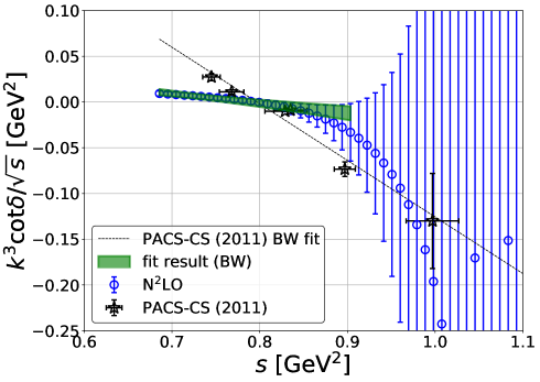
Figure 8: The Breit-Wigner fit for the N²LO phase shifts $k^{3}\cot\delta_{1}(k)/\sqrt{s}$ (blue points). The green band represents the fit with statistical errors and a range of the energy used in the fit. We also show data and Breit-Wigner fit of PACS-CS (2011) Aoki et al. (2011a) by the black points and the dashed line, respectively, for a comparison.

We have checked that resonance parameters remain unchanged within statistical errors even if we add a centrifugal barrier modification as a higher order term in $k^{2}$Von Hippel and Quigg (1972) to the standard Breit-Wigner form in Eq. (23).

IV.3.2 Direct pole search

Theoretically, a resonance state is defined as a pole of the S-matrix on the second Riemann sheet, which provides us the second method to extract resonance parameters in the HAL QCD method. To access the S-matrix in complex energy region, we solve the Schrödinger equation with arguments rotated by $r\to re^{i\theta},k\to ke^{-i\theta}$Giraud et al. (2004); Aguilar and Combes (1971); Balslev and Combes (1971), which reads

$$\left(\frac{d^{2}}{dr^{2}}-\frac{l(l+1)}{r^{2}}-\frac{2\mu e^{2i\theta}V_{0}(e^{i\theta}r)-k^{2}}{1-2\mu V_{2}(e^{i\theta}r)}\right)\phi=0.$$ (26)

The regular solution $\phi$ to this equation behaves at long distances as

$$\phi\to\frac{i}{2}\left[{\mathcal{J}}_{l}(ke^{-i\theta})\hat{h}_{l}^{-}(kr)-{\mathcal{J}}^{*}_{l}(ke^{-i\theta})\hat{h}_{l}^{+}(kr)\right],$$ (27)

where $\hat{h}_{l}^{\pm}(z)=\hat{n}_{l}(z)\pm i\hat{j}_{l}(z)$ are the Riccati-Hankel functions and ${\mathcal{J}}_{l}$ is the Jost function for the angular momentum $l$. The S-matrix on the ray of $ke^{-i\theta}$ can therefore be obtained as

$$s_{l}(ke^{-i\theta})=\frac{{\mathcal{J}}^{*}_{l}(ke^{-i\theta})}{{\mathcal{J}}_{l}(ke^{-i\theta})},$$ (28)

from which we can search a pole position $k_{\rm pole}=|k_{\rm pole}|e^{-i\theta_{\rm pole}}$ by changing an input $\theta$ and $k$. The resonance mass and the decay width are extracted from the pole position $\sqrt{s}_{\rm pole}$ as

$$\sqrt{s}_{\rm pole}=2\sqrt{k_{\rm pole}^{2}+m_{\pi}^{2}}=m_{\rho}-i\Gamma_{\rho}/2,$$ (29)

where the decay width is related to the coupling constant $g_{\rho\pi\pi}$ as

$$g_{\rho\pi\pi}=\sqrt{\frac{6\pi\Gamma_{\rho}m_{\rho}^{2}}{k_{\rho}^{3}}},\quad k_{\rho}:=\sqrt{m_{\rho}^{2}/4-m_{\pi}^{2}}.$$ (30)

The direct pole search gives

$$m_{\rho} = 886(17)(^{+4}_{-1})\ {\rm MeV},$$ (31)

$$\Gamma_{\rho}/2 = 22(8.6)(^{+4.5}_{-0.0})\ {\rm MeV},$$ (32)

$$g_{\rho\pi\pi} = 12.7(2.9)(^{+0.7}_{-0.0}),$$ (33)

where the first errors are statistical while the second ones are systematic errors associated with the short-range behavior of $V_{0}^{\rm N^{2}LO}$.

IV.3.3 Comparison to the previous result

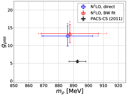
Figure 9: A comparison of N²LO resonance parameters from the direct pole search (blue circle) and the Breit-Wigner fit (red triangle). Vertical and horizontal axes represent the coupling $g_{\rho\pi\pi}$ and the mass $m_{\rho}$, respectively. Statistical (systematic) errors are represented by solid (dashed) bars. Shown together is the result from PACS-CS (2011) Aoki et al. (2011a) (black star). Errors for PACS-CS (2011) are statistical only.

Let us compare our N²LO results with the previous PACS-CS (2011) result using the finite-volume method Aoki et al. (2011a), both of which employ the same gauge configurations. We plot $m_{\rho}$ and $g_{\rho\pi\pi}$ in Fig. 9. While $m_{\rho}$’s are consistent with each other in all three cases, the Breit-Wigner fit, the pole search and the PACS-CS (2011) result, coupling constants in our both results are about twice as large as the previous one. This discrepancy can be clearly seen as a difference in slopes of $k^{3}\cot\delta_{1}/\sqrt{s}$ data at $s<0.9$ GeV² in Fig. 8, which directly correspond to the coupling as $-6\pi/g_{\rho\pi\pi}^{2}$. In particular, a significant disagreement between the lowest energy level in PACS-CS and our data at $s\approx 0.75$ GeV² is a main source of the discrepancy for the slope. We note that the lowest energy level in PACS-CS (2011) is obtained in the laboratory frame with ${\bf P}=(0,0,2\pi/L)$. Since such a low-energy region cannot be covered by the center-of-mass frame employed in this study and the non-locality of the potential in $I=1$ $\pi\pi$ systems turns out to be large, our N²LO approximation is likely to suffer from large truncation errors in the derivative expansion at low energies.

This observation gives us a useful lesson for the study of P-wave (or higher partial wave) resonances by the HAL QCD method with the center-of-mass frame. If the non-locality of the potential happens to be large, the truncation errors could be large at low-energies near the threshold. While a resonance mass is likely to be well reproduced as long as the resonance appears in the energy region accessible in the center-of-mass frame, the decay width (the effective coupling) may suffer from larger systematics since it is sensitive to energy dependence on a much wider range around the resonance. As a possible option to control this systematics, if the resonance mass can be roughly guessed, one may tune lattice parameters such as a box size carefully so as to cover a wide energy range even in the center-of-mass frame. This procedure, however, is difficult in practice and applicability for searches of unknown resonances is also limited. The second option is to establish the existence of a resonance and to estimate its mass by the HAL QCD method in the center-of-mass frame, which is supplemented by the finite-volume method in the laboratory frame to estimate its width reliably. The third option is to perform the HAL QCD method with a combination of both the center-of-mass and laboratory frames. In fact, a theoretical framework has been already proposed for the HAL QCD method in the laboratory frameAoki (2020). While extraction of HAL QCD potentials from NBS wave functions in the laboratory frame is indeed a numerical challenge, the first numerical trial is now ongoing.

V Summary

We study the $I=1$ $\pi\pi$ interaction at $m_{\pi}\approx 411$ MeV, where the $\rho$ meson emerges as the resonance with $m_{\rho}\approx 892$ MeV. We calculate all-to-all propagators by a combination of the one-end trick, the sequential propagator, and the covariant approximation averaging. Thanks to those techniques, we successfully determine the potential in this channel at the N²LO of the derivative expansion for the first time and calculate the resonance parameters of the $\rho$ meson.

The mass and decay width of the $\rho$ resonance are directly extracted from the pole position of the S-matrix, $\sqrt{s}_{\rm pole}=886(17)-i22(9)$, whose real part agrees with the $\rho$ resonance mass in the previous study but whose imaginary part leads to the coupling constant $g_{\rho\pi\pi}$ twice as large as the previous one. Larger coupling $g_{\rho\pi\pi}$ originates from the discrepancy in phase shifts at $s\lesssim 0.75$ GeV², whose energy region cannot be covered in the center-of-mass frame of our lattice setup. This observation provides a useful lesson for studies of P-wave resonances by the HAL QCD method and future direction for the improvement is discussed.

Although the issue above remain to be verified explicitly, the result in this study shows that hadronic resonances which require all-to-all calculations can be investigated with reasonable precisions even at the N²LO level in the HAL QCD method. This study opens new doors toward understanding hadronic resonances by the HAL QCD method, including more challenging systems such as $I=0$ $\pi\pi$ ($\sigma$ resonance), $I=1/2$ $K\pi$ ($\kappa$ resonance) and exotic resonances.

Appendix A The one-end trick

In this appendix, we briefly explain the one-end trickMcNeile and Michael (2006), which enables us to estimate a combination of two all-to-all propagators with a space summation by using a single noisy estimator. Let us consider a combination of quark propagators given by

$$\sum_{\bf y}e^{i{\bf p\cdot y}}D_{f}^{-1}({\bf x}_{1},t_{1};{\bf y},t_{0})\Gamma D_{f^{\prime}}^{-1}({\bf y},t_{0};{\bf x}_{2},t_{2}),$$ (34)

where $D_{f}^{-1}$ is a quark propagator with a flavor $f$, $\Gamma$ is some product of gamma matrices, and $x_{i}=({\bf x}_{i},t_{i})$ are arbitrary. We abbreviate color and spin indices for simplicity. Such a structure typically appears at the source side of correlation functions including meson operators. For example, in the separated diagram in Fig. 10, it appears twice as

$$\begin{split}(+)\sum_{{\bf y_{1},y_{2}}}e^{i{\bf p_{z}\cdot y_{1}}}e^{-i{\bf p_{z}\cdot y_{2}}}&{\rm tr}\left[\underline{D^{-1}({\bf x+r},t;{\bf y_{1}},t_{0})\gamma_{5}D^{-1}({\bf y_{1}},t_{0};{\bf x+r},t)}\gamma_{5}\right]\\ &\times{\rm tr}\left[\underline{D^{-1}({\bf x},t;{\bf y_{2}},t_{0})\gamma_{5}D^{-1}({\bf y_{2}},t_{0};{\bf x},t)}\gamma_{5}\right].\end{split}$$ (35)

The calculation of those structures naively needs two stochastic estimations for each, since each of them contains two all-to-all propagators. The one-end trick, however, utilize the $\gamma_{5}$-Hermiticity of the Dirac operator to estimate that structure with a single noise insertion as follows.

$$\begin{split}\sum_{\bf y}e^{i{\bf p\cdot y}}&D^{-1}(x_{1};{\bf y},t_{0})\Gamma D^{-1}({\bf y},t_{0};x_{2})\\ &=\sum_{\bf y,z}e^{i{\bf p\cdot y}}D^{-1}(x_{1};{\bf y},t_{0})\delta_{\bf y,z}\Gamma D^{-1}({\bf z},t_{0};x_{2})\\ &\approx\sum_{\bf y,z}e^{i{\bf p\cdot y}}D^{-1}(x_{1};{\bf y},t_{0})\left(\frac{1}{N_{\rm r}}\sum_{r=0}^{N_{\rm r}-1}\eta_{[r]}({\bf y})\eta_{[r]}^{{\dagger}}({\bf z})\right)\Gamma D^{-1}({\bf z},t_{0};x_{2})\\ &=\frac{1}{N_{\rm r}}\sum_{r=0}^{N_{\rm r}-1}\left(\sum_{\bf y}D^{-1}(x_{1};{\bf y},t_{0})\eta_{[r]}({\bf y})e^{i{\bf p\cdot y}}\right)\left(\sum_{\bf z}\gamma_{5}D^{-1}(x_{2};{\bf z},t_{0})\gamma_{5}\Gamma^{{\dagger}}\eta_{[r]}({\bf z})\right)^{{\dagger}},\end{split}$$ (36)

where we insert the stochastic estimator $\delta_{\bf y,z}\approx\frac{1}{N_{\rm r}}\sum_{r=0}^{N_{\rm r}-1}\eta_{[r]}({\bf z})\eta_{[r]}^{{\dagger}}({\bf y})$ in the second line and use the $\gamma_{5}$-Hermiticity in the last line. We define ”one-end vectors“ as

$$\xi_{{\bf p},t_{0}[r]}(x) \equiv \sum_{\bf y}D^{-1}(x;{\bf y},t_{0})\eta_{[r]}({\bf y})e^{i{\bf p\cdot y}}$$ (37)

$$\chi_{\Gamma,t_{0}[r]}(x) \equiv \sum_{\bf y}D^{-1}(x;{\bf y},t_{0})\gamma_{5}\Gamma^{{\dagger}}\eta_{[r]}({\bf y}),$$ (38)

then the final expression becomes

$$\sum_{\bf y}D^{-1}({\bf x}_{1},t_{1};{\bf y},t_{0})\Gamma D^{-1}({\bf y},t_{0};{\bf x}_{2},t_{2})\approx\frac{1}{N_{\rm r}}\sum_{r=0}^{N_{\rm r}-1}\xi_{{\bf p},t_{0}[r]}({\bf x}_{1},t_{1})\otimes\chi_{\Gamma,t_{0}[r]}^{{\dagger}}({\bf x}_{2},t_{2})\gamma_{5}.$$ (39)

The one-end vectors $\xi$ and $\chi$ are obtained by solving the linear equation $D\xi=\eta e^{i{\bf p\cdot y}}$ and $D\chi=\gamma_{5}\Gamma^{{\dagger}}\eta$, respectively. The dilution technique for noise reduction can be combined as well. This trick is particularly suitable for the HAL QCD method since it does not introduce any stochastic estimations at the sink side, which otherwise strongly affects spatial dependences of the NBS wave function. Moreover, a numerical cost and stochastic noises are also reduced in accordance with a decrease in the number of noise vectors.

Appendix B Numerical evaluation for each diagram

Here we outline details of numerical evaluation for each diagram calculations in this study. Figure 10 gives representative quark contraction diagrams appearing in the two-pion correlation functions, and the techniques utilized in the evaluations of quark propagator are shown by different colors and symbols. Other diagrams similar to these representatives are calculated similarly.In the following, we assume to employ a single noise vector for each insertion. Color and spin indices are implicit for simplicity as well.

separated diagram

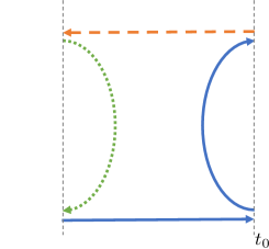
box diagram

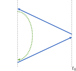
triangle diagram

Figure 10: Representative diagrams appeared in this study. Blue solid, orange dashed and green dotted lines are calculated with the one-end trick, sequential propagator and point-to-all propagator, respectively. Statistical improvement by the CAA is also employed for green dotted lines.

B.1 Separated diagram

As already seen, a separated diagram in Fig. 10 is written as

$$\begin{split}G^{\rm sep}_{{\bf x};t_{0}}({\bf r},t)=(+)\sum_{{\bf y_{1},y_{2}}}e^{i{\bf p_{z}\cdot y_{1}}}e^{-i{\bf p_{z}\cdot y_{2}}}&{\rm tr}\left[D^{-1}({\bf x+r},t;{\bf y_{1}},t_{0})\gamma_{5}D^{-1}({\bf y_{1}},t_{0};{\bf x+r},t)\gamma_{5}\right]\\ &\times{\rm tr}\left[D^{-1}({\bf x},t;{\bf y_{2}},t_{0})\gamma_{5}D^{-1}({\bf y_{2}},t_{0};{\bf x},t)\gamma_{5}\right].\end{split}$$ (40)

By using the one-end trick twice, we obtain

$$G^{\rm sep}_{{\bf x};t_{0}}({\bf r},t)=(+)\sum_{i,j}\left(\chi_{\gamma_{5},t_{0}[r]}^{(i){\dagger}}({\bf x+r},t)\xi_{{\bf p}_{z},t_{0}[r]}^{(i)}({\bf x+r},t)\right)\left(\chi_{\gamma_{5},t_{0}[s]}^{(j){\dagger}}({\bf x},t)\xi_{-{\bf p}_{z},t_{0}[s]}^{(j)}({\bf x},t)\right),$$ (41)

where $i,j$ are indices for dilutions and $r,s$ distinguish independent noise vectors. In practice, the center-of-mass coordinate ${\bf x}$ is averaged over the whole spacetime to improve the statistical errors,

$$G^{\rm sep}_{t_{0}}({\bf r},t)=\frac{1}{L^{3}}\sum_{\bf x}G^{\rm sep}_{{\bf x};t_{0}}({\bf r},t).$$ (42)

.

B.2 Box diagrams

A box diagram shown in Fig. 10 is written as

$$\begin{split}G^{\rm box}_{{\bf x};t_{0}}({\bf r},t)=(-)\sum_{{\bf y_{1},y_{2}}}e^{i{\bf p_{z}\cdot y_{1}}}e^{-i{\bf p_{z}\cdot y_{2}}}&{\rm tr}[D^{-1}({\bf x+r},t;{\bf y_{1}},t_{0})\gamma_{5}D^{-1}({\bf y_{1}},t_{0};{\bf y_{2}},t_{0})\gamma_{5}\\ &\times D^{-1}({\bf y_{2}},t_{0};{\bf x},t)\gamma_{5}D^{-1}({\bf x},t;{\bf r+x},t)\gamma_{5}]\end{split}$$ (43)

For an estimation of this diagram, we first utilize the one-end trick for a summation of ${\bf y_{2}}$,

$$\begin{split}(-)\sum_{i}\sum_{{\bf y_{1}}}e^{i{\bf p_{z}\cdot y_{1}}}&{\rm tr}[D^{-1}({\bf x+r},t;{\bf y_{1}},t_{0})\gamma_{5}\xi_{-{\bf p}_{z},t_{0}[r]}^{(i)}({\bf y_{1}},t_{0})\chi_{\gamma_{5},t_{0}[r]}^{(i){\dagger}}({\bf x},t)D^{-1}({\bf x},t;{\bf r+x},t)\gamma_{5}].\end{split}$$ (44)

We next exactly calculate another all-to-all propagator $D^{-1}({\bf x+r},t;{\bf y_{1}},t_{0})$ by the sequential propagator technique Martinelli and Sachrajda (1989), where we consider a linear equation with a sequential source vector $e^{i{\bf p_{z}\cdot y_{1}}}\gamma_{5}\xi_{-{\bf p}_{z},t_{0}[r]}^{(i)}({\bf y_{1}},t_{0})$ as

$$\left(D\zeta\right)(x)=e^{i{\bf p_{z}\cdot x}}\gamma_{5}\xi_{-{\bf p}_{z},t_{0}[r]}^{(i)}({\bf x},t)\delta_{t,t_{0}},$$ (45)

whose solution $\zeta$ is given by

$$\zeta^{(i)}_{{\bf p_{z}},-{\bf p_{z}},t_{0}[r]}({\bf x},t)=\sum_{{\bf y_{1}}}D^{-1}({\bf x},t;{\bf y_{1}},t_{0})\gamma_{5}\xi_{-{\bf p}_{z},t_{0}[r]}^{(i)}({\bf y_{1}},t_{0})e^{i{\bf p_{z}\cdot y_{1}}}.$$ (46)

Substituting Eq. (46) into Eq. (44), we obtain

$$\begin{split}G^{\rm box}_{{\bf x};t_{0}}({\bf r},t)=(-)\sum_{i}\chi_{\gamma_{5},t_{0}[r]}^{(i){\dagger}}({\bf x},t)H^{-1}({\bf x},t;{\bf r+x},t)\zeta^{(i)}_{{\bf p_{z}},-{\bf p_{z}},t_{0}[r]}({\bf r+x},t),\end{split}$$ (47)

where $H^{-1}$ is an inverse of the hermitized Dirac operator $H=\gamma_{5}D$.

To increase statistics of the box diagrams, instead of an average over all ${\bf x}$ with an additional noisy estimation, we employ the covariant approximation averaging (CAA) for ${\bf x}$, which is given by

$$G^{\rm box,imp}_{{\bf x_{0}};t_{0}}({\bf r},t)=G^{\rm box,exact}_{{\bf x_{0}};t_{0}}({\bf r},t)-G^{\rm box,relaxed}_{{\bf x_{0}};t_{0}}({\bf r},t)+\frac{1}{N_{G}}\sum_{\bf x^{\prime}}G^{\rm box,relaxed}_{{\bf x^{\prime}};t_{0}}({\bf r},t),$$ (48)

where $N_{G}$ is the number of a summation over ${\bf x^{\prime}}$. Here $G^{\rm box,exact/relaxed}$ is defined as

$$\begin{split}G^{\rm box,exact/relaxed}_{{\bf x_{0}};t_{0}}&({\bf r},t)\\ =(-)\sum_{i}&\Biggl{[}\frac{1}{L^{3}}\sum_{\bf x}\sum_{n}^{N_{\rm low}}\frac{1}{\lambda_{n}}\chi_{\gamma_{5},t_{0}[r]}^{(i){\dagger}}({\bf x},t)v^{(n)}({\bf x},t)v^{(n){\dagger}}({\bf x+r},t)\zeta^{(i)}_{{\bf p_{z}},-{\bf p_{z}},t_{0}[r]}({\bf r+x},t)\\ &+\chi_{\gamma_{5},t_{0}[r]}^{(i){\dagger}}({\bf x_{0}},t)H_{\rm high,exact/relaxed}^{-1}({\bf x_{0}},t;{\bf r+x_{0}},t)\zeta^{(i)}_{{\bf p_{z}},-{\bf p_{z}},t_{0}[r]}({\bf r+x_{0}},t)\Biggr{]},\end{split}$$ (49)

where $\lambda_{n}$ and $v^{(n)}$ are the $n$-th eigenvalue and eigenvector of $H$, respectively, $N_{\rm low}$ is the number of low-eigenmodes used in the CAA, while $H_{\rm high,exact/relaxed}^{-1}$ is an inverse of $H$ projected onto a space spanned by remaining high-eigenmodes solved with a tight/relaxed stopping condition. Since $\chi$ and $\zeta$ are already solved with high precision, we only relax a precision of the sink-to-sink propagator (green dotted line in Fig. 10). Furthermore, we averaged over all ${\bf x}$ in the low-eigenmode part to maximize statistics.

B.3 Triangle diagram

A triangle diagram shown in Fig. 10 is written as

$$G^{\rm tri}_{{\bf x};t_{0}}({\bf r},t)=(-)\sum_{\bf y}{\rm tr}[D^{-1}({\bf r+x},t;{\bf y},t_{0})\gamma_{3}D^{-1}({\bf y},t_{0};{\bf x},t)\gamma_{5}D^{-1}({\bf x},t;{\bf r+x},t)\gamma_{5}].$$ (50)

Using the one-end trick for a summation over ${\bf y}$, we obtain

$$\begin{split}G^{\rm tri}_{{\bf x};t_{0}}({\bf r},t)=(-)\sum_{i}\chi_{\gamma_{3},t_{0}[r]}^{(i){\dagger}}({\bf x},t)H^{-1}({\bf x},t;{\bf r+x},t)\xi^{(i)}_{{\bf 0},t_{0}[r]}({\bf r+x},t).\end{split}$$ (51)

As in the case of the box diagram, we employ the CAA for ${\bf x}$, which gives an improved triangle diagram as

$$G^{\rm tri,imp}_{{\bf x_{0}};t_{0}}({\bf r},t)=G^{\rm tri,exact}_{{\bf x_{0}};t_{0}}({\bf r},t)-G^{\rm tri,relaxed}_{{\bf x_{0}};t_{0}}({\bf r},t)+\frac{1}{N_{G}}\sum_{\bf x^{\prime}}G^{\rm tri,relaxed}_{{\bf x^{\prime}};t_{0}}({\bf r},t),$$ (52)

where

$$\begin{split}G^{\rm tri,exact/relaxed}_{{\bf x_{0}};t_{0}}&({\bf r},t)\\ =(-)\sum_{i}&\Biggl{[}\frac{1}{L^{3}}\sum_{\bf x}\sum_{n}^{N_{\rm low}}\frac{1}{\lambda_{n}}\chi_{\gamma_{5},t_{0}[r]}^{(i){\dagger}}({\bf x},t)v^{(n)}({\bf x},t)v^{(n){\dagger}}({\bf x+r},t)\xi^{(i)}_{{\bf 0},t_{0}[r]}({\bf r+x},t)\\ &+\chi_{\gamma_{5},t_{0}[r]}^{(i){\dagger}}({\bf x_{0}},t)H_{\rm high,exact/relaxed}^{-1}({\bf x_{0}},t;{\bf r+x_{0}},t)\xi^{(i)}_{{\bf 0},t_{0}[r]}({\bf r+x_{0}},t)\Biggr{]}.\end{split}$$ (53)

Appendix C Smeared-sink scheme

In this appendix, we discuss properties of the smeared-sink scheme in detail.

C.1 Point-sink scheme vs smeared-sink scheme in $I=1$ $\pi\pi$ system

To see why the smeared-sink scheme is needed for the $I=1$ $\pi\pi$ potential, let us compare potentials between the point-sink scheme and the smeared-sink scheme. Figure 11 (left) shows the $I=1$ $\pi\pi$ potentials calculated from the $\pi\pi$-type source with $N_{\rm conf}=18$ ($\times$ 64 time slice average). While the potential in the point-sink scheme show large non-smooth and scattered behavior at short distances, which makes a fit to this potential difficult, such behavior is absent for the potential in the smeared-sink scheme. Since the potential in the point-sink scheme without box diagrams does not show such non-smooth behavior(Fig. 11 (right)), it is probably caused by box diagrams, which contain quark creation/annihilation processes.

We suspect that this non-smooth and scattered structure is related to a singular behavior of the NBS wave function at short distances, caused by quark creation/annihilation processes in this channel. According to the argument by the operator product expansionAoki et al. (2010b, c, 2012b, 2012c, 2013b), the $I=1$ $\pi\pi$ operator at the sink strongly couples to the $\rho$ operator at short distance, whose mass dimension is lower than the $\pi\pi$ operator by 3, and the NBS wave function behaves as $\psi_{W}({\bf r})\sim\frac{1}{r^{3}}Y_{l=1,m=0}(\Omega_{\bf r})$ at short distances. This implies that the NBS wave function is highly localized and singular around the origin, which is indeed the case in the point-sink scheme, as seen in Fig.12 (Left). Since data available around the origin are restricted on a discrete space, it is difficult to extract a potential smoothly from such a localized wave function by a discretized Laplacian. In the smeared-sink scheme, on the other hand, a singular structure of the NBS wave function at short distances is much milder as seen in Fig.12 (Right), so that the potential reconstructed from discrete data shows a smoother behavior at short distances. We also expect similar behaviors of HAL QCD potentials at short distances generally for other systems which contain quark creation/annihilation diagrams.

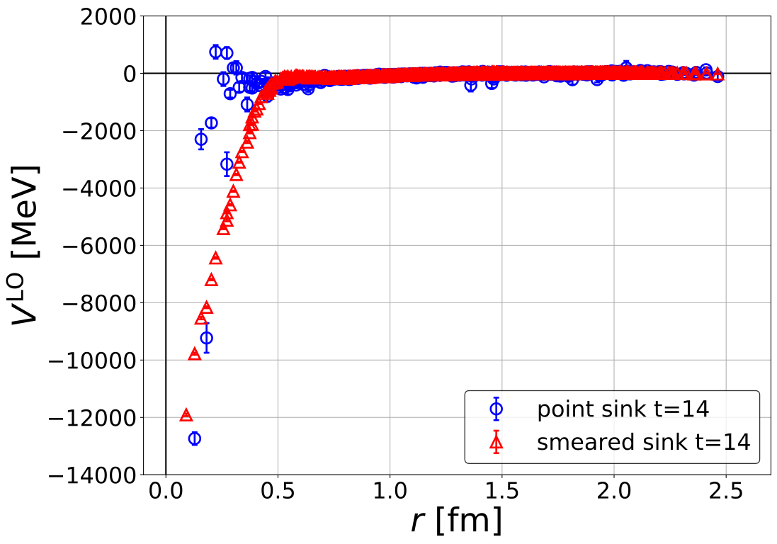
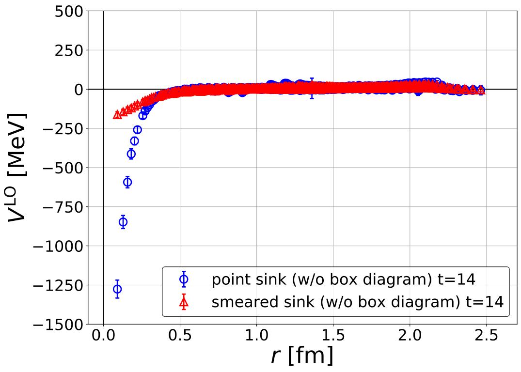
Figure 11: A comparison in $I=1$ $\pi\pi$ potential between two schemes at $t=14$. (Left) The effective LO potentials from the $\pi\pi$-type source operator. Blue (red) points show data in the point-sink (smeared-sink) scheme. (Right) Those from the NBS wave function without box diagrams.

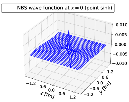
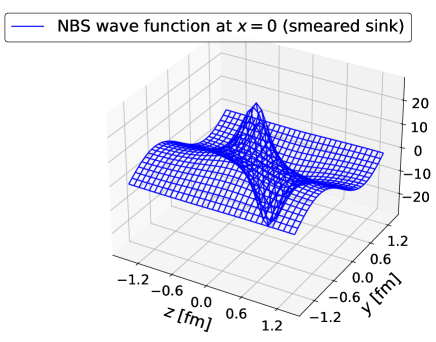
Figure 12: The NBS wave function at $x=0$ in the point-sink scheme (Left) and the smeared-sink scheme (Right).

C.2 Effect on the derivative expansion

The previous HAL QCD study with the LapH method Kawai et al. (2018) has revealed that the LapH sink-smearing significantly enhances non-localities of HAL QCD potentials, which makes the derivative expansion less reliable. Therefore we would like to check whether our sink-smearing scheme given in eq.(2) is free from such a problem. For this purpose, we calculate $I=2$ $\pi\pi$ potential in both point-sink and smeared-sink schemes and compare LO phase shifts between the two schemes.

Calculations of NBS wave functions in both schemes are performed by using the one-end trick with full color/spin dilution and $s2$ space dilution for a single $Z_{4}$ noise. A number of configuration is $N_{\rm conf}=10$ ($\times 64$ timeslice average), and statistical errors are estimated by the jackknife method with bin-size 1.

Figure 13(left) shows effective LO potentials at $t=14$. Potentials between two schemes show significantly different behaviors only at short distances, which however do not affect phase shifts at $\sqrt{s}<1200$ MeV, as plotted in Fig. 13 (right). Thus the smeared-sink does not enhance non-locality of the $I=2$ $\pi\pi$ potential in this energy region. Since a relevant energy range for the $\rho$ resonance in this study is well covered by this energy region ($\sqrt{s}<1200$ MeV), we also expect that non-locality of the $I=1$ $\pi\pi$ potential is not enhanced by the smeared-sink scheme, either.

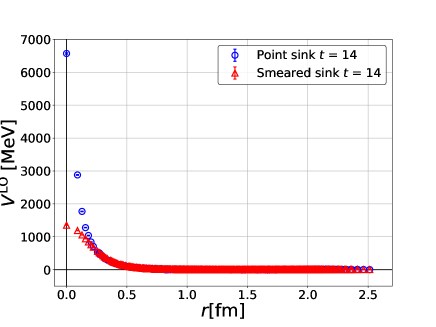
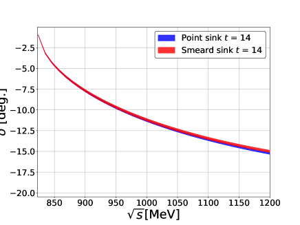
Figure 13: A comparison between point-sink and smeared-sink schemes for the $I=2$ $\pi\pi$ system. (Left) Effective LO potentials. Blue (red) points show data in the point-sink (smeared-sink) scheme. (Right) Corresponding phase shifts.

Appendix D Assumptions for the analysis of $V_{2}^{\rm N^{2}LO}$

In this appendix, we discuss assumptions made for the analysis of $V_{2}^{\rm N^{2}LO}$. The effective LO potential is related to the exact non-local potential as

$$V_{i}^{\rm LO}=V_{0}+V_{2}\frac{\nabla^{2}R_{i}}{R_{i}}+V_{4}\frac{\nabla^{4}R_{i}}{R_{i}}+\cdots.$$ (54)

Let us consider a case where the N⁴LO and higher terms are negligibly small. In this case, the effective LO potential and the exact N²LO potential $V_{0},V_{2}$ can be related by

$$V_{i}^{\rm LO}=V_{0}+V_{2}\frac{\nabla^{2}R_{i}}{R_{i}},\quad{(i=A,B)},$$ (55)

which leads to

$$\Delta V^{\rm LO}\equiv V_{A}^{\rm LO}-V_{B}^{\rm LO}=V_{2}\left(\frac{\nabla^{2}R_{A}}{R_{A}}-\frac{\nabla^{2}R_{B}}{R_{B}}\right)\equiv V_{2}\Delta\left(\frac{\nabla^{2}R}{R}\right).$$ (56)

Using this relation, we find

$$\Delta\left(\frac{\nabla^{2}R}{R}\right)=0\ {\rm at}\ r=r_{0}\ \Rightarrow\ \Delta V^{\rm LO}=0\ {\rm and}\ \Delta V_{\rm ene}^{\rm LO}=0\ {\rm at}\ r=r_{0},$$ (57)

where $\Delta V_{\rm ene}^{\rm LO}\equiv\Delta V^{\rm LO}-\Delta\left(\frac{\nabla^{2}R}{R}\right)/2\mu$. Therefore, if $\Delta\left(\frac{\nabla^{2}R}{R}\right)$ vanishes at $r_{0},r_{1},\cdots$, both $\Delta V^{\rm LO}$ and $\Delta V_{\rm ene}^{\rm LO}$ must become zero also at those points.

Figure 14 shows data of $\Delta V^{\rm LO}$, $\Delta\left(\frac{\nabla^{2}R}{R}\right)$, and $\Delta V_{\rm ene}^{\rm LO}$ in this study. While $\Delta\left(\frac{\nabla^{2}R}{R}\right)$ has a single zero, $\Delta V^{\rm LO}$ and $\Delta V_{\rm ene}^{\rm LO}$ have zeros at slightly different positions, probably due to the neglected higher order effects in $\Delta V^{\rm LO}$ and $\Delta V_{\rm ene}^{\rm LO}$. We assume in our N²LO analysis that our data are well described without N⁴LO and higher order terms so that $\Delta V^{\rm LO}$, $\Delta\left(\frac{\nabla^{2}R}{R}\right)$ and $\Delta V_{\rm ene}^{\rm LO}$ share a common zero point. This assumption motivates us to employ a non-singular function which satisfies $2\mu V_{2}^{\rm N^{2}LO}-1\ (=2\mu\Delta V_{\rm ene}^{\rm LO}/\Delta\left(\frac{\nabla^{2}R}{R}\right))\ <0$ at all $r$ in the fit of $V_{2}^{\rm N^{2}LO}$.

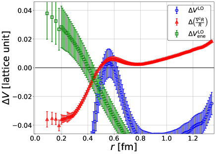
Figure 14: Behaviors of $\Delta V^{\rm LO}$(blue circles), $\Delta(\nabla^{2}R/R)$(red triangles) and $\Delta V_{\rm ene}^{\rm LO}$(green squares).

Appendix E Energy-dependent local N²LO potential

Here, we discuss our N²LO potential in a different point of view, an energy-dependent local form. We can convert the energy-independent non-local N²LO potential $U^{\rm N^{2}LO}=V^{\rm N^{2}LO}_{0}+V^{\rm N^{2}LO}_{2}\nabla^{2}$ to an energy-dependent local form $V^{\rm N^{2}LO}(r;k)$ as Iritani et al. (2019b)

$$V^{\rm N^{2}LO}(r;k)=\frac{V^{\rm N^{2}LO}_{0}-k^{2}V^{\rm N^{2}LO}_{2}}{1-m_{\pi}V^{\rm N^{2}LO}_{2}}.$$ (58)

Figure 15 shows this energy-dependent local potentials with the centrifugal term at several energies: near threshold ($\sqrt{s}=830$ MeV), near the ground state energy in the center-of-mass frame ($\sqrt{s}=910$ MeV), and at higher energy ($\sqrt{s}=1050$ MeV). At low energies, we observe that the attractive pocket of the $V^{\rm N^{2}LO}(r;k)$ is smaller than that of the LO potential $V^{\rm LO}_{\rho}$ which makes N²LO phase shifts smaller than LO phase shifts. Around the CM ground state energy, $V^{\rm N^{2}LO}(r;k)$ and $V^{\rm LO}_{\rho}$ are almost identical, since $V^{\rm LO}_{\rho}$ is obtained from correlators saturated by that state. At high-energy region, a difference between $V^{\rm N^{2}LO}(r;k)$ and $V^{\rm LO}_{\rho}$ becomes larger in all ranges. The significant improvement by the N²LO analysis for the phase shifts at high energies can be understood from this difference.

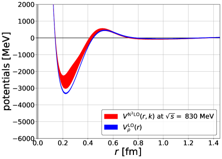
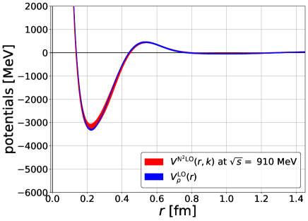
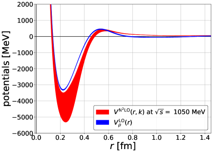
Figure 15: Energy-dependent local N²LO potentials. (Upper left) near threshold ($\sqrt{s}=830$ MeV). (Upper right) near the CM frame ground state energy ($\sqrt{s}=910$ MeV). (Lower left) larger energy ($\sqrt{s}=1050$ MeV). For a comparison, we show the effective LO potential with $\rho$-type source.

References

- Luscher (1991) M. Luscher, Nucl. Phys. B 354, 531 (1991).
- Rummukainen and Gottlieb (1995) K. Rummukainen and S. A. Gottlieb, Nucl. Phys. B 450, 397 (1995), arXiv:hep-lat/9503028 .
- Hansen and Sharpe (2012) M. T. Hansen and S. R. Sharpe, Phys. Rev. D 86, 016007 (2012), arXiv:1204.0826 [hep-lat] .
- Ishii et al. (2007) N. Ishii, S. Aoki, and T. Hatsuda, Phys. Rev. Lett. 99, 022001 (2007), arXiv:nucl-th/0611096 .
- Aoki et al. (2010a) S. Aoki, T. Hatsuda, and N. Ishii, Prog. Theor. Phys. 123, 89 (2010a), arXiv:0909.5585 [hep-lat] .
- Aoki (2011) S. Aoki (HAL QCD Collaboration), Prog. Part. Nucl. Phys. 66, 687 (2011), arXiv:1107.1284 [hep-lat] .
- Ishii et al. (2012) N. Ishii, S. Aoki, T. Doi, T. Hatsuda, Y. Ikeda, T. Inoue, K. Murano, H. Nemura, and K. Sasaki (HAL QCD Collaboration), Phys. Lett. B 712, 437 (2012), arXiv:1203.3642 [hep-lat] .
- Briceno et al. (2018) R. A. Briceno, J. J. Dudek, and R. D. Young, Rev. Mod. Phys. 90, 025001 (2018), arXiv:1706.06223 [hep-lat] .
- Aoki et al. (2011a) S. Aoki et al. (PACS-CS Collaboration), Phys. Rev. D 84, 094505 (2011a), arXiv:1106.5365 [hep-lat] .
- Feng et al. (2011) X. Feng, K. Jansen, and D. B. Renner, Phys. Rev. D 83, 094505 (2011), arXiv:1011.5288 [hep-lat] .
- Lang et al. (2011) C. B. Lang, D. Mohler, S. Prelovsek, and M. Vidmar, Phys. Rev. D 84, 054503 (2011), [Erratum: Phys.Rev.D 89, 059903 (2014)], arXiv:1105.5636 [hep-lat] .
- Dudek et al. (2013) J. J. Dudek, R. G. Edwards, and C. E. Thomas (Hadron Spectrum Collaboration), Phys. Rev. D 87, 034505 (2013), [Erratum: Phys.Rev.D 90, 099902 (2014)], arXiv:1212.0830 [hep-ph] .
- Wilson et al. (2015) D. J. Wilson, R. A. Briceno, J. J. Dudek, R. G. Edwards, and C. E. Thomas, Phys. Rev. D 92, 094502 (2015), arXiv:1507.02599 [hep-ph] .
- Alexandrou et al. (2017) C. Alexandrou, L. Leskovec, S. Meinel, J. Negele, S. Paul, M. Petschlies, A. Pochinsky, G. Rendon, and S. Syritsyn, Phys. Rev. D 96, 034525 (2017), arXiv:1704.05439 [hep-lat] .
- Andersen et al. (2019) C. Andersen, J. Bulava, B. Hörz, and C. Morningstar, Nucl. Phys. B 939, 145 (2019), arXiv:1808.05007 [hep-lat] .
- Werner et al. (2020) M. Werner et al. (ETM Collaboration), Eur. Phys. J. A 56, 61 (2020), arXiv:1907.01237 [hep-lat] .
- Fischer et al. (2020) M. Fischer, B. Kostrzewa, M. Mai, M. Petschlies, F. Pittler, M. Ueding, C. Urbach, and M. Werner (ETM Collaboration), (2020), arXiv:2006.13805 [hep-lat] .
- Iritani et al. (2019a) T. Iritani, S. Aoki, T. Doi, T. Hatsuda, Y. Ikeda, T. Inoue, N. Ishii, H. Nemura, and K. Sasaki (HAL QCD Collaboration), JHEP 03, 007 (2019a), arXiv:1812.08539 [hep-lat] .
- Aoki et al. (2011b) S. Aoki, N. Ishii, T. Doi, T. Hatsuda, Y. Ikeda, T. Inoue, K. Murano, H. Nemura, and K. Sasaki (HAL QCD Collaboration), Proc. Japan Acad. B 87, 509 (2011b), arXiv:1106.2281 [hep-lat] .
- Aoki and Doi (2020) S. Aoki and T. Doi, Front. in Phys. 8, 307 (2020), arXiv:2003.10730 [hep-lat] .
- Ikeda et al. (2016) Y. Ikeda, S. Aoki, T. Doi, S. Gongyo, T. Hatsuda, T. Inoue, T. Iritani, N. Ishii, K. Murano, and K. Sasaki (HAL QCD Collaboration), Phys. Rev. Lett. 117, 242001 (2016), arXiv:1602.03465 [hep-lat] .
- Ikeda (2018) Y. Ikeda (HAL QCD Collaboration), J. Phys. G 45, 024002 (2018), arXiv:1706.07300 [hep-lat] .
- Sasaki et al. (2020) K. Sasaki et al. (HAL QCD Collaboration), Nucl. Phys. A 998, 121737 (2020), arXiv:1912.08630 [hep-lat] .
- Peardon et al. (2009) M. Peardon, J. Bulava, J. Foley, C. Morningstar, J. Dudek, R. G. Edwards, B. Joo, H.-W. Lin, D. G. Richards, and K. J. Juge (Hadron Spectrum Collaboration), Phys. Rev. D 80, 054506 (2009), arXiv:0905.2160 [hep-lat] .
- Foley et al. (2005) J. Foley, K. Jimmy Juge, A. O’Cais, M. Peardon, S. M. Ryan, and J.-I. Skullerud, Comput. Phys. Commun. 172, 145 (2005), arXiv:hep-lat/0505023 .
- Kawai et al. (2018) D. Kawai, S. Aoki, T. Doi, Y. Ikeda, T. Inoue, T. Iritani, N. Ishii, T. Miyamoto, H. Nemura, and K. Sasaki (HAL QCD Collaboration), PTEP 2018, 043B04 (2018), arXiv:1711.01883 [hep-lat] .
- Kawai (2018) D. Kawai (HAL QCD Collaboration), EPJ Web Conf. 175, 05007 (2018).
- Akahoshi et al. (2019) Y. Akahoshi, S. Aoki, T. Aoyama, T. Doi, T. Miyamoto, and K. Sasaki, PTEP 2019, 083B02 (2019), arXiv:1904.09549 [hep-lat] .
- Akahoshi et al. (2020) Y. Akahoshi, S. Aoki, T. Aoyama, T. Doi, T. Miyamoto, and K. Sasaki, PTEP 2020, 073B07 (2020), arXiv:2004.01356 [hep-lat] .
- McNeile and Michael (2006) C. McNeile and C. Michael (UKQCD Collaboration), Phys. Rev. D 73, 074506 (2006), arXiv:hep-lat/0603007 .
- Martinelli and Sachrajda (1989) G. Martinelli and C. T. Sachrajda, Nucl. Phys. B 316, 355 (1989).
- Shintani et al. (2015) E. Shintani, R. Arthur, T. Blum, T. Izubuchi, C. Jung, and C. Lehner, Phys. Rev. D 91, 114511 (2015), arXiv:1402.0244 [hep-lat] .
- Aoki (2020) S. Aoki, in 37th International Symposium on Lattice Field Theory (2020) arXiv:2001.01076 [hep-lat] .
- Aoki et al. (2013a) S. Aoki, N. Ishii, T. Doi, Y. Ikeda, and T. Inoue, Phys. Rev. D 88, 014036 (2013a), arXiv:1303.2210 [hep-lat] .
- Aoki et al. (2012a) S. Aoki, T. Doi, T. Hatsuda, Y. Ikeda, T. Inoue, N. Ishii, K. Murano, H. Nemura, and K. Sasaki (HAL QCD Collaboration), PTEP 2012, 01A105 (2012a), arXiv:1206.5088 [hep-lat] .
- Murano et al. (2014) K. Murano, N. Ishii, S. Aoki, T. Doi, T. Hatsuda, Y. Ikeda, T. Inoue, H. Nemura, and K. Sasaki (HAL QCD Collaboration), Phys. Lett. B 735, 19 (2014), arXiv:1305.2293 [hep-lat] .
- Iritani et al. (2019b) T. Iritani, S. Aoki, T. Doi, S. Gongyo, T. Hatsuda, Y. Ikeda, T. Inoue, N. Ishii, H. Nemura, and K. Sasaki (HAL QCD Collaboration), Phys. Rev. D 99, 014514 (2019b), arXiv:1805.02365 [hep-lat] .
- Aoki et al. (2009) S. Aoki et al. (PACS-CS Collaboration), Phys. Rev. D 79, 034503 (2009), arXiv:0807.1661 [hep-lat] .
- Iwasaki (1985) Y. Iwasaki, Nucl. Phys. B 258, 141 (1985).
- Sheikholeslami and Wohlert (1985) B. Sheikholeslami and R. Wohlert, Nucl. Phys. B 259, 572 (1985).
- Miyamoto et al. (2020) T. Miyamoto, Y. Akahoshi, S. Aoki, T. Aoyama, T. Doi, S. Gongyo, and K. Sasaki, Phys. Rev. D 101, 074514 (2020), arXiv:1906.01987 [hep-lat] .
- Von Hippel and Quigg (1972) F. Von Hippel and C. Quigg, Phys. Rev. D 5, 624 (1972).
- Giraud et al. (2004) B. G. Giraud, K. Kato, and A. Ohnishi, J. Phys. A 37, 11575 (2004), arXiv:nucl-th/0503049 .
- Aguilar and Combes (1971) J. Aguilar and J. M. Combes, Commun. Math. Phys. 22, 269 (1971).
- Balslev and Combes (1971) E. Balslev and J. M. Combes, Commun. Math. Phys. 22, 280 (1971).
- Amagasa et al. (2015) T. Amagasa et al., J. Phys. Conf. Ser. 664, 042058 (2015).
- Ueda et al. (2014) S. Ueda, S. Aoki, T. Aoyama, K. Kanaya, H. Matsufuru, S. Motoki, Y. Namekawa, H. Nemura, Y. Taniguchi, and N. Ukita, J. Phys. Conf. Ser. 523, 012046 (2014).
- Kanamori and Matsufuru (2018) I. Kanamori and H. Matsufuru (2018) arXiv:1811.00893 [hep-lat] .
- Aoki et al. (2010b) S. Aoki, J. Balog, and P. Weisz, JHEP 05, 008 (2010b), arXiv:1002.0977 [hep-lat] .
- Aoki et al. (2010c) S. Aoki, J. Balog, and P. Weisz, JHEP 09, 083 (2010c), arXiv:1007.4117 [hep-lat] .
- Aoki et al. (2012b) S. Aoki, J. Balog, and P. Weisz, New J. Phys. 14, 043046 (2012b), arXiv:1112.2053 [hep-lat] .
- Aoki et al. (2012c) S. Aoki, J. Balog, and P. Weisz, Prog. Theor. Phys. 128, 1269 (2012c), arXiv:1208.1530 [hep-lat] .
- Aoki et al. (2013b) S. Aoki, J. Balog, T. Doi, T. Inoue, and P. Weisz, Int. J. Mod. Phys. E 22, 1330012 (2013b), arXiv:1302.0185 [hep-lat] .