Evaluating Modules in Graph Contrastive Learning

Abstract.

The recent emergence of contrastive learning approaches facilitates the application on graph representation learning (GRL), introducing graph contrastive learning (GCL) into the literature. These methods contrast semantically similar and dissimilar sample pairs to encode the semantics into node or graph embeddings. However, most existing works only performed model-level evaluation, and did not explore the combination space of modules for more comprehensive and systematic studies. For effective module-level evaluation, we propose a framework that decomposes GCL models into four modules: (1) a sampler to generate anchor, positive and negative data samples (nodes or graphs); (2) an encoder and a readout function to get sample embeddings; (3) a discriminator to score each sample pair (anchor-positive and anchor-negative); and (4) an estimator to define the loss function. Based on this framework, we conduct controlled experiments over a wide range of architectural designs and hyperparameter settings on node and graph classification tasks. Specifically, we manage to quantify the impact of a single module, investigate the interaction between modules, and compare the overall performance with current model architectures. Our key findings include a set of module-level guidelines for GCL, e.g., simple samplers from LINE and DeepWalk are strong and robust; an MLP encoder associated with Sum readout could achieve competitive performance on graph classification. Finally, we release our implementations and results as OpenGCL, a modularized toolkit that allows convenient reproduction, standard model and module evaluation, and easy extension. OpenGCL is available at https://github.com/thunlp/OpenGCL.

1. Introduction

Learning representations with better utilization of unlabelled data has been a crucial issue in deep learning. Among such approaches, self-supervised learning designs heuristic pretext tasks to learn representations with self-generated labels (Liu et al., 2020). Recent advances in self-supervised learning mainly concentrate on contrastive learning, which discriminates semantically similar and dissimilar sample pairs following the InfoMax principle (Linsker, 1988). Sustainable progress has been made in domains such as computer vision (Chen et al., 2020; He et al., 2020; Oord et al., 2018) and natural language processing (Devlin et al., 2019; Kong et al., 2020; Mikolov et al., 2013).

In the literature of graph representation learning (GRL), traditional models directly train node embeddings by graph structure. DeepWalk (Perozzi et al., 2014) assumes that concurrences of nodes in random walks can reveal structural similarity. LINE (Tang et al., 2015) presumes the first-order and second-order similarities of neighboring nodes. With the success of graph neural networks (GNNs) (Kipf and Welling, 2017), graph auto-encoder (GAE) (Kipf and Welling, 2016) combines feature and structure information, and makes a significant advance. Recently, there also emerge several contrastive learning models (Hassani and Ahmadi, 2020; Sun et al., 2020; Velickovic et al., 2019; You et al., 2020a; Zhu et al., 2021b) which contrast between different graph views. These methods achieve state-of-the-art performance and even outperform some semi-supervised models (Hassani and Ahmadi, 2020; Zhu et al., 2021b). However, despite the potential of self-supervised GRL, current analysis and evaluation are limited to model level. In the following paragraphs, we will demonstrate this issue and stress the importance of module-level analysis and evaluation.

Firstly, current self-supervised GRL models are developed independently. They mainly concentrate on designing new pretext tasks and their architectural differences and similarities are barely explored. For example, the training objectives of LINE-2nd (Tang et al., 2015) and GAE (Kipf and Welling, 2016) both presume that neighboring nodes are analogous and optimize the inner product similarity (see appendix for details). As we will discuss later, both models can fit into the contrastive learning framework, with a mere difference in graph encoder. However, a rough model-level analysis will neglect these internal model architectures. Therefore, to get better understandings of graph contrastive learning, we propose a modularized framework, and show how eight classical and state-of-the-art self-supervised GRL models can be fit into the framework. Our framework interprets graph constrastive learning with 4 disjoint modules: (1) The context sampler, which chooses anchor, positive, and negative data samples; (2) the graph encoder and readout function, which project samples to low-dimensional representations; (3) the discriminator, which assigns a score to each anchor-context pair; (4) the estimator, which provides a contrastive loss.

Secondly, model-level evaluation is also insufficient for a thorough analysis. As the models are specific combinations of disjoint modules, module-level evaluation allows us to gain more insights about how to learn good representations by effective architectural design. In this work, we conduct thorough evaluations over various modules by controlled experiments. We manage to investigate the impact of each single module, explore the pairwise combination effect of modules, and compare our best module combinations with state-of-the-art models. Our key results include: (1) simple LINE and DeepWalk samplers are surprisingly powerful and robust; (2) the combination of Sum readout function and MLP encoder are comparable with GNN-based architectures on graph classification; (3) the best model architectures from our framework can achieve state-of-the-art performances, which illustrates the potential of the framework.

In addition, most graph contrastive learning model implementations are not fully modularized as well, making it difficult for module-level evaluation. Thus, a modularized and extendable toolkit is also needed. To deal with this issue, we develop OpenGCL, an open-source toolkit for the implementation and evaluation of modularized graph contrastive learning model.

We sum up our contributions as follows:

1. Framework. We propose a modularized framework for GCL and analyze the distinctions and similarities of several typical models under the framework.

2. Evaluation. We conduct extensive experiments on a wide range of architectural designs, hyperparameter settings, and benchmarks. The experimental results and analysis help us explore the key factors in learning good representations.

3. Toolkit. We release OpenGCL, an open-source toolkit for graph contrastive learning. OpenGCL allows modularized implementation and evaluation of various models, encouraging further research on GCL.

2. Related Work

2.1. Contrastive Learning

For contrastive learning, the key issue is the augmentation strategy to generate similar pairs. In the computer vision domain, additional views are usually produced by randomly cropping or flipping the original image (Chen et al., 2020; Oord et al., 2018), by which most semantics of images are preserved.

Graphs, however, usually have latent semantics, which brings challenges when designing contrastive learning models. Early methods mainly focused on node-level contrast, which managed to find similar context nodes for a given anchor node (Kipf and Welling, 2016; Perozzi et al., 2014; Tang et al., 2015). The context nodes are selected locally from neighborhoods or random walks and the contrastive learning principle is entailed implicitly. Motivated by Deep InfoMax (Hjelm et al., 2019), some methods (Hassani and Ahmadi, 2020; Sun et al., 2020; Velickovic et al., 2019) proposed to contrast local and global representations for learning multi-scale graph structure representations. Most recently, models with newly designed augmentation strategies like node dropping and attribute masking were proposed (You et al., 2020a; Zhu et al., 2021b).

2.2. Frameworks of GRL Models

The idea of unifying GRL models has been studied from various perspectives (Hamilton et al., 2017; Qiu et al., 2018; You et al., 2020a). Conventional shallow embedding models can be summarized by matrix factorization (Qiu et al., 2018; Yang et al., 2017). However, the matrix factorization framework cannot easily incorporate feature information. Therefore, a more comprehensive encoder-decoder framework (Hamilton et al., 2017) was introduced to interpret algorithms based on matrix factorization, random walk and graph neural networks.

In terms of contrastive learning, You et al. (You et al., 2020a) proposed a contrastive framework for graph-level representation learning, which mainly focused on the design of different pretext tasks. Some recent surveys (Liu et al., 2021; Wu et al., 2021; Xie et al., 2021) also summarized graph contrastive learning models, but they did not compare the effect of different modules by experiments. Recently, there is a concurrent work (Zhu et al., 2021a) which also discussed and evaluated graph contrastive learning. Compared with this work, we conduct controlled random experiments to comprehensively evaluate modules. Moreover, we investigate the pairwise combination effect and overall performance, which makes our work more systematic.

2.3. Evaluation of GRL Models

Multiple research works concentrated on evaluating various GRL models (Dwivedi et al., 2020; Errica et al., 2020; Mesquita et al., 2020; Shchur et al., 2018; You et al., 2020b). Shchur et al. (Shchur et al., 2018) explored the impact of dataset split for GNN models and concluded that different dataset splits lead to dramatically different model performances. Some works (Dwivedi et al., 2020; Hu et al., 2020) further proposed new multi-scale benchmarks for appropriate GNN evaluation. On graph classification task, Errica et al. (Errica et al., 2020) provided a rigorous comparison for graph classification. Mesquita et al. (Mesquita et al., 2020) challenged all the local pooling algorithms and demonstrated that local graph pooling is not crucial for learning graph representations. However, the aforementioned research works are limited to model-level evaluation of existing models. We break down full models into modules, which helps us find out what plays a bigger role inside a model. You et al. (You et al., 2020b) discussed the architectural designs of GNN models, such as batch size and the activation function. By abundant experiments, they provided comprehensive guidelines for GNN designs over various tasks. In contrast, we focus on module-level architectures rather than network designs.

3. Preliminaries

Given a graph $\mathcal{G}=(\mathcal{V},\mathcal{E})$, where $\mathcal{V}$ is the vertex set and $\mathcal{E}$ is the edge set, the graph structure can be represented by an adjacency matrix $\mathbf{A}$. In some cases, nodes in graph $\mathcal{G}$ are associated with features $\mathbf{X}$. Graph representation learning aims to map graph substructures (nodes, edges, subgraphs etc.) to low-dimensional embeddings.

After we get the node representations, we can summarize the graph-level representations by a readout function. The learned representations are often used in downstream graph learning tasks. In this paper, we focus on node classification and graph classification tasks.

4. Proposed Framework

We propose a modularized framework for graph contrastive learning, which consists of four modules:

1. Context sampler. Following the priors inside data distributions, a context sampler provides an augmentation mechanism on graph data, which generates semantically similar (positive) and dissimilar (negative) contexts for the given anchor data point. For each batch, the context sampler chooses one anchor $x$, one positive context $k^{+}$ and $N$ negative contexts $\{k^{-}_{i}\}_{i=1}^{N}$.

2. Graph encoder. The encoder Enc maps selected data points to distributional vectors. More specifically, we learn node embeddings by node encoders, and get graph embeddings by a following readout function.

3. Discriminator. The discriminator Disc scores each anchor-context pair in the batch according to the agreement between them. The score function $f$ is defined as

   (1) $$f(x,k)=\texttt{Disc}(\texttt{Enc}(x),\texttt{Enc}(k)).$$

4. Mutual information estimator. The mutual information estimator $I_{\texttt{Est}}$ defines the loss function, which enforces the representations of positive pairs (anchor and positive contexts) to be close, and those of negative pairs (anchor and negative contexts) to be orthogonal. We define the optimization objective as follows:

   (2) $$\max\mathbb{E}_{x,k^{+},\{k^{-}_{i}\}_{i=1}^{N}}\left[I_{\texttt{Est}}\left(f(x,k^{+});\left\{f(x,k^{-}_{i})\right\}_{i=1}^{N}\right)\right].$$

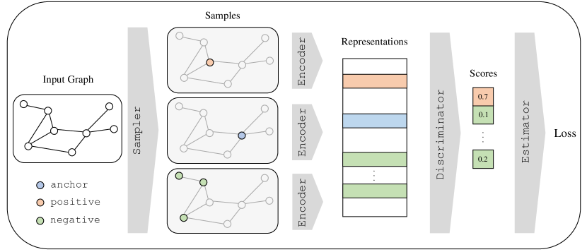
Figure 1. Our framework of GCL. (1) The anchor, positive and negative data samples are selected by the sampler following an underlying prior data distribution. (2) A shared graph encoder is then applied to project data samples to low-dimensional representations. (3) The discriminator scores anchor-context pairs. (4) The estimator brings positive pairs closer and separates negative pairs apart by a contrastive loss.

Next we give a detailed discussion over possible instantiations of each module.

4.1. Sampler

One major distinction in different sampling strategies lies in the “views” of data. Samplers in LINE (Tang et al., 2015), GAE (Kipf and Welling, 2016) and DeepWalk (Perozzi et al., 2014) focus on the same local view of graph structure, where samples come from nodes in the original graph. Samplers in DGI (Velickovic et al., 2019) and InfoGraph (Sun et al., 2020) adapt the idea of Deep InfoMax (Hjelm et al., 2019) to graph domain; they maximize the mutual information between global and local views in the original dataset by contrasting nodes against graphs. More recently, MVGRL (Hassani and Ahmadi, 2020), GCA (Zhu et al., 2021b) and GraphCL (You et al., 2020a) develop samplers that generate views by augmenting the given graphs; the corresponding nodes and/or graphs in different views are thought to be similar. Out of the eight mentioned models, we conclude six samplers based on their views and sampling processes:

1. Sampler in LINE (and GAE) selects neighboring nodes as anchors and positive samples. Negative samples are random nodes in the dataset.

2. Sampler in DeepWalk performs random walk and applies Skip-gram model to the resulting paths, where anchor-positive pairs are taken by sliding windows. Negative samples are random nodes in the dataset.

3. Sampler in DGI (and InfoGraph) selects graphs as anchors. Nodes are seen as positive samples if they are from the anchor graph, and as negative samples if not. In datasets with one single graph, negative nodes are chosen from a “negative graph” which is generated by shuffling node features.

4. Sampler in MVGRL is similar to that in DGI, except that the positive and negative samples are nodes from diffusion graphs like personalized PageRank (Page et al., 1999).

5. Sampler in GCA takes up edge dropping and attribute masking as augmentation strategies and contrasts nodes between graph augmentations $G_{A}$ and $G_{B}$ ($A$ and $B$ are randomly selected augmentation strategies). It takes one node in $G_{A}$ as anchor, the corresponding node in $G_{B}$ as positive sample, and all the other nodes from both graphs as negative samples.

6. Sampler in GraphCL contrasts global augmentative views. It adapts edge dropping, attribute masking, node dropping and subgraph sampling for augmentation. Augmentations $G_{A}$ and $G_{B}$ from one graph are selected as anchor and positive sample, while augmentation $G^{\prime}_{B}$ from another graph is the negative sample.

4.2. Encoder

4.2.1. Node Encoder

A node encoder, which converts nodes to embeddings, is the first part of a encoder. Conventional GRL models (DeepWalk, LINE) usually learn node embeddings directly, thus the encoders are simply lookup tables. However, lookup tables initialize node embeddings randomly and independently, which can not utilize node feature and graph topology structure. With the proposal of GCN, many recent models (GAE, DGI) adopt GCN as their encoders to capture neighborhood dependency and node feature information. Some variants of GCN are also widely adopted. GAT (Velickovic et al., 2018) uses the attention mechanism to better model the relative influence between node pairs. Graph isomorphism network (GIN) (Xu et al., 2019) is proved to be as powerful as the Weisfeiler-Lehman graph isomorphism test thus is more expressive than GCN. Instead of average aggregator, GIN sums over neighborhood hidden representations to update the target node’s hidden representation. GIN could capture the size information of graphs. Therefore, InfoGraph and GraphCL alter GCN with GIN as it better suits graph-level tasks.

4.2.2. Readout Function

Additionally, for models that need to learn graph-level representations, a readout function is required to summarize node representations. Two basic readout functions are average and sum functions. DGI takes the average of node embeddings to get graph embeddings. InfoGraph and GraphCL sum over node embeddings to encode graph size information. To utilize the mid-layer node representations, following JK-Net (Xu et al., 2018), MVGRL concatenates the summation of node representation in each encoder layer for graph representations.

4.3. Discriminator

The discriminator measures the similarity of node or graph pairs. Intuitively, inner product is the most straightforward score function, which is selected by most models. DGI adopts a bilinear discriminator instead to score between local and global (node and graph) representations.

4.4. Estimator

Several mutual information estimators have been introduced in previous works. Based on Jensen-Shannon divergence (Nowozin et al., 2016), the objective functions in DeepWalk, LINE, GAE, DGI, InfoGraph and MVGRL are binary cross-entropy over positive and negative scores:

(3) $$I_{\texttt{JSD}}=\sigma(f(x,k^{+}))+\frac{1}{N}\sum_{i=1}^{N}\sigma\left(-f(x,k^{-}_{i})\right),$$

where $\sigma$ is the LogSigmoid function, which is defined as

(4) $$\text{LogSigmoid}(x)=\log\frac{1}{1+\exp(-x)}$$

Based on Noise-Contrastive Estimation of KL-divergence, InfoNCE estimator is also commonly used in contrastive learning (Oord et al., 2018), which is defined as

(5) $$I_{\texttt{InfoNCE}}=\log\frac{\exp{\left(f(x,k^{+})\right)}}{\exp{\left(f(x,k^{+})\right)}+\sum_{i=1}^{N}\exp{\left(f(x,k^{-}_{i})\right)}}.$$

GCA and GraphCL use InfoNCE estimator. Note that InfoNCE estimator usually adopts in-batch negative samples, where all samples except positive ones in the same mini-batch are selected as negative samples.

Table 1. Summary of algorithms in our framework.

Model	Encoder Node Encoder Readout Function		Sampler	Discriminator	Estimator
DeepWalk (Perozzi et al., 2014)	Lookup	-	Random walk	Inner product	JSD
LINE (Tang et al., 2015)	Lookup	-	Neighboring nodes	Inner product	JSD
GAE (Kipf and Welling, 2016)	GCN	-	Neighboring nodes	Inner product	JSD
DGI (Velickovic et al., 2019)	GCN	Mean	Local-global views	Bilinear	JSD
MVGRL (Hassani and Ahmadi, 2020)	GCN	JK-Net	Diffusion	Inner product	JSD
InfoGraph (Sun et al., 2020)	GIN	Sum	Local-global views	Inner product	JSD
GraphCL (You et al., 2020a)	GIN	Sum	Augmentative global	Inner product	InfoNCE
GCA (Zhu et al., 2021b)	GCN	-	Augmentative local	Inner product	InfoNCE

We summarize how several influential algorithms consistently fit into our framework. These models differ in the choice of encoders, samplers, discriminators and estimators. As shown in Table 1, our framework provides an alternative view for self-supervised GRL. In experiments, we factorize these methods and control modules to find out the key issues for learning high-quality representations.

5. OpenGCL

To foster our experiments and further researches, we develop an open-source toolkit OpenGCL. OpenGCL is specifically designed for graph contrastive learning with several important features:

1. Modularization. We implement OpenGCL with factorized modules following our framework, which allows users to create any module combination within one command line. Users can reproduce existing models and easily choose the best combinations for specific tasks and datasets.

2. Standardized evaluation. We enable convenient model-level and module-level evaluation on multiple tasks and datasets. With simple scripts, users can generate, run and manage experiments.

3. Extensibility. Users may easily implement their modules, such as new samplers or graph pooling readout functions. New tasks and datasets can also be imported with ease.

All of the following experiments and analyses are conducted with OpenGCL.

6. Experimental Setup

In this section, we describe the modules, hyperparameters, benchmark datasets and design in our experiments.

6.1. Modules

We list the ranges for each module in Table 3. To explore the most important model architectures, we consider the module instantiations widely-used in current researches. Note that we name the samplers with their corresponding models. LINE and GAE, DGI and InfoGraph adopt the same samplers, so we denote them as LINE and DGI samplers. We also include MLP and GAT (Velickovic et al., 2018) as encoders, because they are also widely used in GRL literature.

6.2. Hyperparameters

We select the most essential hyperparameters: embedding size, network layers in the encoder, number of negative samples in the sampler, and learning rate and batch size in the optimization process. The hyperparameter values are chosen from a rigorous range based on experience from current literature. As for hyperparameters in specific modules, like window size in DeepWalk sampler, we fix them at reasonable values. We train each model using Adam optimizer (Kingma and Ba, 2014) for 500 epochs, and early stop training when there are 3 consecutive loss increase epochs.

• Embedding size. We adopt 64 and 128.

• Learning rate is fixed at 0.01.

• Hidden dimensions. The hidden dimensions are the same as the embedding size.

• Encoder layers. The number of encoder layers range from $\{1,2,3,4\}$.

• Negative samples. InfoNCE uses in-batch negative samples. JSD uses 1 negative sample for each positive sample.

• Sample size. To avoid OOM issues, we sample subgraphs for large graphs. The sample size is 5000.

• Batch size. For both node and graph tasks, we constrain the total amount of nodes in a batch. In contrastive learning, large batches are usually considered to be beneficial, so we fix batch size at 4096 nodes. For multi-graph datasets, we select graphs so that the number of all nodes in one batch does not exceed 4096; each graph with more than 4096 nodes (maximum 5000 due to graph sampling) makes up one batch.

• Normalization. Following the common settings, we normalize embeddings for InfoNCE estimator.

Table 2. Dataset statistics

Task	Dataset	#Graphs	Avg. #Nodes	Avg. #Edges	#Features	#Classes
Node Classification	Amazon-C	1	13,752	245,861	767	10
	Amazon-P	1	7,650	119,081	745	8
	CiteSeer	1	3,327	4,732	3,703	6
	Coauthor-CS	1	18,333	81,894	6,805	15
	Coauthor-Phy	1	34,493	247,962	8,415	5
	Cora	1	2,708	5,429	1,433	7
	PubMed	1	19,717	44,338	500	3
	WikiCS	1	11,701	216,123	300	10
Graph Classification	IMDB-B	1,000	19.77	193.06	-	2
	IMDB-M	1,500	13.00	65.93	-	3
	PTC-MR	344	14.29	14.69	-	2
	MUTAG	188	17.93	19.79	-	2
	Reddit-B	2,000	508.52	497.75	-	2

6.3. Datasets

We evaluate the quality of learned node and graph embeddings on downstream classification tasks. For node classification, we adopt eight standard benchmark datasets: Cora, Citeseer, and Pubmed (Sen et al., 2008) are three widely-used citation networks. Features in Cora and Citeseer are binary word vectors, while in Pubmed, nodes are associated with tf-idf weighted word vectors. Wiki-CS (Mernyei and Cangea, 2020) is a newly proposed reference network. Nodes are computer science articles from Wikipedia and edges are hyperlinks linking the articles. Features are the average GloVe (Pennington et al., 2014) word embeddings for each article and nodes are labeled by their branches in the field. Amazon-Computers and Amazon-Photo (Shchur et al., 2018) are built from Amazon co-purchase graph (McAuley et al., 2015). Nodes represent products and edges mean two products are frequently bought together. Features of the nodes are bag-of-words vectors of product reviews. Nodes are labeled by product categories. Coauthor-CS and Coauthor-Physics (Shchur et al., 2018) are co-authorship graphs based on the Microsoft Academic Graph (Sinha et al., 2015). Nodes are authors and they are connected if they co-author a paper. Features are bag-of-words vectors of authors’ keywords. Nodes are labeled by research fields. We split each dataset into train (20%), validation (10%) and test (70%) data.

For graph classification, we use another five common datasets: MUTAG and PTC-MR (Chen et al., 2007) are bioinfomatic datasets. MUTAG collects mutagenic aromatic and heteroaromatic nitro compounds and PTC-MR contains chemical compounds that reports the carcinogenicity for rats. IMDB-B, IMDB-B and IMDB-M (Yanardag and Vishwanathan, 2015) are collaboration networks for movies. Each graph represent a ego-network for an actor/actress. Nodes are actors/actresses and they are linked if they appear in the same movie. Graphs are labeled by the genres they are generated. We use an 80%/10%/10% split for this task. The detailed dataset statistics can be found in Table 2. Following state-of-the-art approaches (Hassani and Ahmadi, 2020; Sun et al., 2020; Velickovic et al., 2019), we train a logistic regression classifier with five-fold cross-validation.

6.4. Experiment Design

To quantitatively evaluate the impact of various architectural designs, we conduct controlled random search experiments conditioned on module instantiations following (You et al., 2020b). For instance, suppose we want to explore the impact of different estimators on a specific task. First we randomly draw $M$ experiments from the full setup space with $I_{\texttt{Est}}=I_{\texttt{InfoNCE}}$. With other modules fixed, we then alter their estimators with $I_{\texttt{Est}}=I_{\texttt{JSD}}$ to get another $M$ experiments, which generates $M$ pairs of experiments for us. To compare InfoNCE with JSD estimator across datasets, we rank experiments inside a pair by their performances and analyze the ranking distribution. Experiments in one pair may rank the same if their performance difference is less than 0.01. In this work, we set $M=100$.

Table 3. Search space of modules and hyperparameters.

	Module	Hyperparameter
Encoder	Node: Lookup, MLP, GCN, GAT, GIN Readout: Mean, Sum	embedding size, network layers
Sampler	DeepWalk, LINE, DGI, MVGRL, GCA, GraphCL	negative samples
Discriminator	Inner product, Bilinear
Estimator	InfoNCE, JSD
Optimization		learning rate, batch size

7. Results and Discussion

In this section, we discuss the experimental results. To conduct a thorough analysis for over 3,400 experimental runs, we consider three perspectives:

1. Single module. Through controlled experiments, we can analyze the impact of each single module. From this perspective, we aim to find how each module would contribute to the final performance.

2. Pairwise combination. Apart from single module evaluation, we also explore the effect of pairwise module combination. From this perspective, we try to investigate how the modules interact with each other and find out the best-performing pairs.

3. Full model. We focus on the assembled model performances on various datasets and compare them with existing models. From this perspective, we want to demonstrate that our framework is potent to produce state-of-the-art models.

7.1. Single Module Evaluation

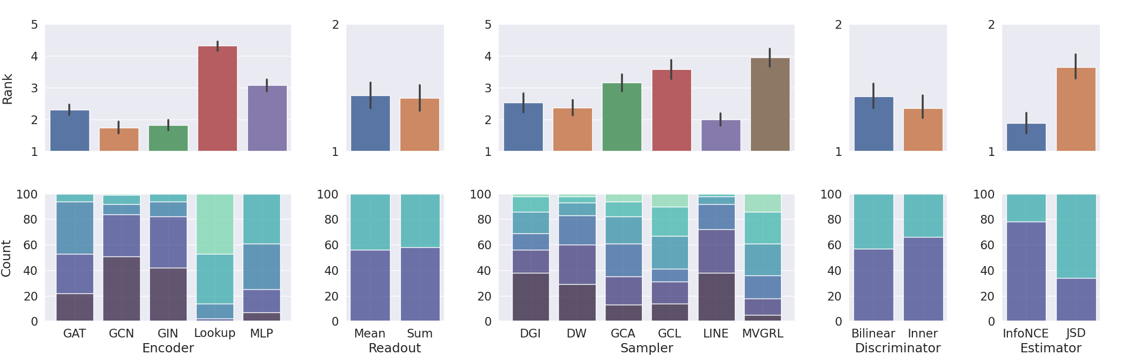
(a) Node classification.

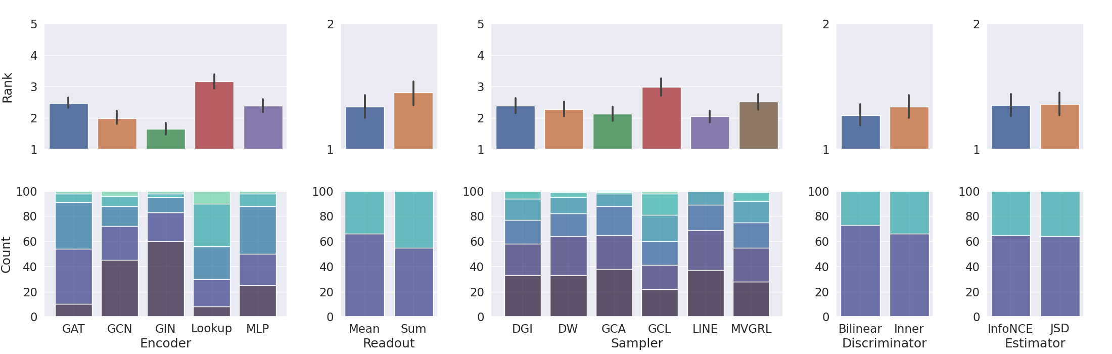
(b) Graph classification.

Figure 2. Module ranking results. Lower is better. Top: average ranking and confidence, lower is better. Bottom: ranking distribution. Lower rankings are darker. Sums of the same ranks may differ in case of ties.

We present the ranking results in Figure 2. From the results, we have the following observations.

Table 4. Top: Memory and time cost of encoders. Bottom: Time cost of samplers.

Dataset	Encoder	Size (KB)	Time (ms)	GPU Memory (MB)
Cora	GAT	869	4.34	215.45
	GCN	502	2.45	30.56
	GIN	502	3.06	46.08
	MLP	501	2.25	30.56
	Lookup	827	1.94	15.04
MUTAG	GAT	139	4.85	304.37
	GCN	136	2.84	14.44
	GIN	137	2.91	14.54
	MLP	136	2.26	14.44
	Lookup	997	2.26	14.35

Dataset	Sampler	Time (ms)	# Samples	Time/Sample ($\mu$s)
Cora	GraphCL	45.44	3686	12.33
	DGI	9.26	4096	2.26
	GCA	35.72	8192	4.36
	MVGRL	1342.05	4096	327.65
	LINE	121.72	13264	9.18
	DW	578.92	2700	214.42
MUTAG	GraphCL	177.98	5983	29.75
	DGI	37.61	6742	5.58
	GCA	76.87	13484	5.70
	MVGRL	49.29	6742	7.31
	LINE	123.24	10813	11.40
	DW	635.45	3360	189.12

7.1.1. Node classification.

(1) For node encoders, GNN encoders are generally better than MLP and Lookup encoders. Under most cases, GCN and GIN stay at the top. This demonstrates the effectiveness of GNNs in node classification. In the meantime, GAT is not as robust as GCN and GIN, which aligns previous works (e.g.  (Shchur et al., 2018)).

(2) For readout functions, Mean and Sum readout functions are roughly as good, which is reasonable because in the node classification task, node representations are not sensitive to the size of the entire graph.

(3) For samplers, DGI and LINE samplers have the highest probabilities to rank 1st. Additionally, DeepWalk and LINE samplers are surprisingly robust compared to the newly proposed samplers, since they rarely drop out of top 4.

(4) For discriminators, Inner product discriminator is slightly better than Bilinear. But the difference is marginal.

(5) For estimators, an interesting observation is that InfoNCE estimator outperforms JSD estimator by a large margin, even though the former is rarely used in node classification. This observation aligns with recent research (Chen et al., 2020) that using more negative samples benefits contrastive representation learning. We highlight this as useful for future research and suggest using InfoNCE rather than JSD for GCL practitioners.

7.1.2. Graph classification.

(1) For node encoders, due to the strong expressive power, GIN stands out among encoders and rank 1st in 60% of experimental runs. However, the advantages of GNN encoders shrink, and MLP even get equal average ranking with GAT. We believe this is mainly caused by the relatively small sizes and simple structures of graphs in this task.

(2) For readout functions and discriminators,Mean readout function and Bilinear discriminator are slightly better than their alternatives, but the gaps are close. There are no definitive conclusions for the best modules.

(3) For samplers, the ranking results of various samplers are close, and all the average rankings lie within 3. Considering the consistent robustness and simplicity, we can conclude that DeepWalk and LINE samplers are good choices for both tasks.

7.1.3. Efficiency Analysis.

Apart from performance, we also care about the efficiency of each module, which is essential for real-world deployment and application. In this section, we compare the memory and time cost of different encoders and samplers, the most time-consuming components, to reveal the most and least efficient modules. To evaluate time and space (CUDA memory) complexity, we test the time and GPU usage of the encoders and samplers on Cora and MUTAG. We select LINE as baseline and then changed encoder or sampler one at a time. For encoders, we consider the size of parameters, the time and CUDA memory cost in forward propagation. For samplers, we count the time and number of samples. The results are listed in Table  4; GPU usage of samplers is not listed since we did not use GPU for sampling. Also, since samplers vary on numbers of sample created, we focus on the average time cost per sample.

We can see that all encoders other than the lookup table share a similar size of parameters, but the GAT encoder takes up more than 20 times of GPU memory than the other encoders, along with a significantly slower calculation process. Given that, GAT is the least efficient and memory-saving encoder.

On the other hand, certain samplers behave differently on different graphs. MVGRL is fast on small graphs but dramatically slow on larger graphs, which means that it is hard to perform difussion efficiently on larges graphs. DeepWalk is slow on performing random walks, and it also samples the least nodes among all samplers; Considering the amount of sampled nodes, DGI, GCA, and LINE are three most efficient samplers. GCA and LINE sample large numbers of nodes at high speeds, which is beneficial for large-scale graph contrastive learning

7.2. Pairwise Combination Evaluation

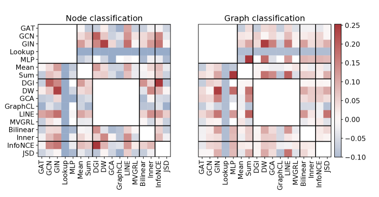
Figure 3. Heatmap of module combination performance $\text{Comb}(x,y)$ for top 10% ranked runs. Warmer colors in square $(x,y)$ indicate the combination of $x$ and $y$ performs better.

To evaluate pairwise combination effect of modules, we group experimental runs by datasets and rank their scores respectively. Then we focus on the top ranked performances of each module combination. Specifically, we collect experimental runs with top $t\%$ scores on each dataset to get a best-$t\%$ pool. For a module pair $(x,y)$, $p_{t}(x,y)$ denotes the probability for it to enter the best-$t\%$ pool, where

(6) $$p_{t}(x,y)=\frac{\#\text{Experimental runs in best-}t\%\ \text{with}\ (x,y)}{\#\text{Experimental runs with}\ (x,y)},$$

and we use $\text{Comb}(x,y)=p_{t}(x,y)-t\%$ to represent the performance of $(x,y)$. Intuitively, $\text{Comb}(x,y)$ measures the probability difference between experiments with $(x,y)$ and the average. Figure 3 shows the heatmap when $t=10$. The diagonal blocks are masked, since only different kinds of modules can be combined. Our following analysis consists of both macro and micro views: the overall effect of one module on other modules, and the pairwise combination influence of specific modules. The macro view can also be seen as the evaluation of a single module in terms of top ranked experimental runs, which can complement the analysis in previous subsection.

Table 5. Best model architecture and baseline on each dataset. The architecture is shown as (Encoder, Readout, Sampler, Discriminator, Estimator).

Dataset	Best sampled architecture	Bestscore	Best baseline	Best score of baseline
Amazon-C	(GCN, Sum, DGI, Bilinear, InfoNCE)	0.861	GAE	0.839
Amazon-P	(GIN, Mean, LINE, Bilinear, InfoNCE)	0.920	GAE	0.912
CiteSeer	(GIN, Mean, DeepWalk, Inner, InfoNCE)	0.708	GAE	0.680
Coauthor-CS	(GAT, Mean, LINE, Inner, JSD)	0.940	GCA	0.931
Coauthor-Phy	(GAT, Mean, DeepWalk, Inner, JSD)	0.956	GCA	0.955
Cora	(GAT, Mean, LINE, Inner, InfoNCE)	0.853	GAE	0.816
PubMed	(GIN, Sum, DeepWalk, Bilinear, InfoNCE)	0.831	GAE	0.830
WikiCS	(GAT, Sum, LINE, Inner, InfoNCE)	0.773	GCA	0.762
IMDB-B	(GCN, Mean, MVGRL, Inner, InfoNCE)	0.729	InfoGraph	0.685
IMDB-M	(GIN, Mean, LINE, Inner, InfoNCE)	0.530	InfoGraph	0.483
MUTAG	(GCN, Mean, DeepWalk, Bilinear, JSD)	0.868	MVGRL	0.842
PTC-MR	(MLP, Sum, DeepWalk, Bilinear, JSD)	0.710	MVGRL	0.681
Reddit-B	(GIN, Sum, DeepWalk, Bilinear, JSD)	0.780	MVGRL	0.729

7.2.1. Node classification.

From the macro view, GCN and GIN encoders, LINE sampler and InfoNCE estimator generally incorporate well with other modules and show positive effects to the system. From the micro view, GCN works well with DGI sampler and GIN favors DeepWalk sampler. As for estimators and samplers, InfoNCE is especially preferable for DGI sampler. We observe that DGI and MVGRL perform better with Bilinear discriminator, while DeepWalk, GCA and LINE work better with Inner product discriminator. This is reasonable because DGI and MVGRL contrast local and global views, which requires alignment between representations.

7.2.2. Graph classification.

From the macro view, readout functions become more important, since graph representations are needed for downstream tasks. Sum readout is generally better than Mean readout for getting high scores. Note that this does not conflict with our previous conclusions in Section 7.1, because here we only consider the best-$t\%$ pool. From the micro view, there are two obvious beneficial combinations: (1) GIN and DeepWalk sampler. This couple is powerful on both tasks, and we attribute this to the utilization of both neighborhood and random walk messages. (2) MLP and Sum readout. This finding is also remarkable, since it indicates that MLP encoder with Sum readout is comparable with GNN-based encoders on current graph classification task. Mesquita et al. (Mesquita et al., 2020) gave a possible explanation that most GNN encoders quickly lead to smooth node representations on small graphs.

7.3. Full Model Evaluation

To highlight that our framework has the potential to find high-performance model architectures, we compare the best models from our experimental runs with the mentioned baseline models, which include LINE, DeepWalk, GAE, DGI, MVGRL and GCA for node classification and DGI, InfoGraph, MVGRL and GraphCL for graph classification. The baseline models are implemented with OpenGCL by assembling their modules. For baseline models, we exhaustively enumerate the entire hyperparameter space from the same range of previous experiments and select the best ones on each dataset. For a fair comparison, we further sample our experiments to match the number of experimental runs with baseline models.

From Table 5, we observe that for each dataset, there exists an assembled model that outperforms the baseline models. The results reveal that searching in the architecture space could be more effective than the hyperparameter space. Note that due to the differences in dataset splits, tricks and hyperparameters, the baseline results are not exactly the same as those reported in the original papers.

The best model architectures imply that GNN encoders are nearly universal components. It is rather impressive that LINE and DeepWalk samplers occur in the best models on 11 out of 13 datasets. This again supports our conclusion that simple samplers can outperform newly proposed samplers when associated with appropriate modules.

8. Conclusion

Despite the rapid growth of graph contrastive learning models, very few works concentrate on which components are crucial in these models. In this paper, we evaluate modules in graph contrastive learning by extensive experimental studies, which has been mostly overlooked in previous works. Our results quantify the impact of each single module and pairwise combination. We find that powerful encoders such as GCN and GIN contribute to a substantial fraction of recent progress while samplers should be revisited for their benefits. Furthermore, the full model evaluation shows that our framework has the potential to generate SOTA model architectures. To foster rigorous comparison methods, we develop OpenGCL as a standard and extensible evaluation toolkit for future research.

Limitations. As our work mainly focuses on modularized evaluation of current models, we do not pay much attention to hyperparameter tuning, and the selected hyperparameter space is limited. Also, the lack of theoretical analysis prevents us from deeper understandings. In the future, a finer hyperparameter search, more fine-grained submodule-level evaluation, and theoretical analysis may lead to more insightful observations and explanations.

References

- (1)
- Chen et al. (2007) J. Chen, E. Linstead, S. J. Swamidass, and P. Baldi D. Wang. 2007. ChemDB Update-full-Text Search and Virtual Chemical Space. Bioinformatics 23 (2007), 2348–2351.
- Chen et al. (2020) Ting Chen, Simon Kornblith, Mohammad Norouzi, and Geoffrey E. Hinton. 2020. A Simple Framework for Contrastive Learning of Visual Representations. In Proceedings of ICML. 1597–1607.
- Devlin et al. (2019) Jacob Devlin, Ming-Wei Chang, Kenton Lee, and Kristina Toutanova. 2019. BERT: Pre-training of Deep Bidirectional Transformers for Language Understanding. In Proceedings of NAACL-HIT. 4171–4186.
- Dwivedi et al. (2020) Vijay Prakash Dwivedi, Chaitanya K Joshi, Thomas Laurent, Yoshua Bengio, and Xavier Bresson. 2020. Benchmarking graph neural networks. arXiv preprint arXiv:2003.00982 (2020).
- Errica et al. (2020) Federico Errica, Marco Podda, Davide Bacciu, and Alessio Micheli. 2020. A Fair Comparison of Graph Neural Networks for Graph Classification. In Proceedings of ICLR.
- Hamilton et al. (2017) William L. Hamilton, Rex Ying, and Jure Leskovec. 2017. Representation Learning on Graphs: Methods and Applications. IEEE Data Eng. Bull. 40, 3 (2017), 52–74.
- Hassani and Ahmadi (2020) Kaveh Hassani and Amir Hosein Khas Ahmadi. 2020. Contrastive Multi-View Representation Learning on Graphs. In Proceedings of ICML. PMLR, 4116–4126.
- He et al. (2020) Kaiming He, Haoqi Fan, Yuxin Wu, Saining Xie, and Ross B. Girshick. 2020. Momentum Contrast for Unsupervised Visual Representation Learning. In Proceedings of CVPR. 9726–9735.
- Hjelm et al. (2019) R. Devon Hjelm, Alex Fedorov, Samuel Lavoie-Marchildon, Karan Grewal, Philip Bachman, Adam Trischler, and Yoshua Bengio. 2019. Learning deep representations by mutual information estimation and maximization. In Proceedings of ICLR.
- Hu et al. (2020) Weihua Hu, Matthias Fey, Marinka Zitnik, Yuxiao Dong, Hongyu Ren, Bowen Liu, Michele Catasta, and Jure Leskovec. 2020. Open Graph Benchmark: Datasets for Machine Learning on Graphs. In Proceedings of NeurIPS.
- Kingma and Ba (2014) Diederik P Kingma and Jimmy Ba. 2014. Adam: A method for stochastic optimization. arXiv preprint arXiv:1412.6980 (2014).
- Kipf and Welling (2016) Thomas N Kipf and Max Welling. 2016. Variational graph auto-encoders. In NIPS Workshop on Bayesian Deep Learning. 3 pages.
- Kipf and Welling (2017) Thomas N Kipf and Max Welling. 2017. Semi-supervised classification with graph convolutional networks. In Proceedings of ICLR. 14 pages.
- Kong et al. (2020) Lingpeng Kong, Cyprien de Masson d’Autume, Lei Yu, Wang Ling, Zihang Dai, and Dani Yogatama. 2020. A Mutual Information Maximization Perspective of Language Representation Learning. In Proceedings of ICLR.
- Linsker (1988) Ralph Linsker. 1988. Self-Organization in a Perceptual Network. Computer 21, 3 (1988), 105–117.
- Liu et al. (2020) Xiao Liu, Fanjin Zhang, Zhenyu Hou, Zhaoyu Wang, Li Mian, Jing Zhang, and Jie Tang. 2020. Self-supervised learning: Generative or contrastive. arXiv preprint arXiv:2006.08218 (2020).
- Liu et al. (2021) Yixin Liu, Shirui Pan, Ming Jin, Chuan Zhou, Feng Xia, and Philip S Yu. 2021. Graph Self-Supervised Learning: A Survey. arXiv preprint arXiv:2103.00111 (2021).
- McAuley et al. (2015) Julian McAuley, Christopher Targett, Qinfeng Shi, and Anton Van Den Hengel. 2015. Image-based recommendations on styles and substitutes. In Proceedings of SIGIR. 43–52.
- Mernyei and Cangea (2020) Péter Mernyei and Cătălina Cangea. 2020. Wiki-cs: A wikipedia-based benchmark for graph neural networks. In ICML Workshop on Graph Representation Learning and Beyond.
- Mesquita et al. (2020) Diego P. P. Mesquita, Amauri H. Souza Jr., and Samuel Kaski. 2020. Rethinking pooling in graph neural networks. In Proceedings of NeurIPS.
- Mikolov et al. (2013) Tomás Mikolov, Ilya Sutskever, Kai Chen, Gregory S. Corrado, and Jeffrey Dean. 2013. Distributed Representations of Words and Phrases and their Compositionality. In Proceedings of NIPS. 3111–3119.
- Nowozin et al. (2016) Sebastian Nowozin, Botond Cseke, and Ryota Tomioka. 2016. f-gan: Training generative neural samplers using variational divergence minimization. In Proceedings of NIPS. 271–279.
- Oord et al. (2018) Aaron van den Oord, Yazhe Li, and Oriol Vinyals. 2018. Representation learning with contrastive predictive coding. arXiv preprint arXiv:1807.03748 (2018).
- Page et al. (1999) Lawrence Page, Sergey Brin, Rajeev Motwani, and Terry Winograd. 1999. The PageRank citation ranking: Bringing order to the web. Technical Report. Stanford InfoLab.
- Pennington et al. (2014) Jeffrey Pennington, Richard Socher, and Christopher D Manning. 2014. Glove: Global vectors for word representation. In Proceedings of EMNLP. 1532–1543.
- Perozzi et al. (2014) Bryan Perozzi, Rami Al-Rfou, and Steven Skiena. 2014. DeepWalk: online learning of social representations. In Proceedings of SIGKDD. ACM, 701–710.
- Qiu et al. (2018) Jiezhong Qiu, Yuxiao Dong, Hao Ma, Jian Li, Kuansan Wang, and Jie Tang. 2018. Network Embedding as Matrix Factorization: Unifying DeepWalk, LINE, PTE, and node2vec. In Proceedings of WSDM. 459–467.
- Sen et al. (2008) Prithviraj Sen, Galileo Namata, Mustafa Bilgic, Lise Getoor, Brian Galligher, and Tina Eliassi-Rad. 2008. Collective classification in network data. AI magazine 29, 3 (2008), 93–93.
- Shchur et al. (2018) Oleksandr Shchur, Maximilian Mumme, Aleksandar Bojchevski, and Stephan Günnemann. 2018. Pitfalls of graph neural network evaluation. arXiv preprint arXiv:1811.05868 (2018).
- Sinha et al. (2015) Arnab Sinha, Zhihong Shen, Yang Song, Hao Ma, Darrin Eide, Bo-June Hsu, and Kuansan Wang. 2015. An overview of microsoft academic service (mas) and applications. In Proceedings of WWW. 243–246.
- Sun et al. (2020) Fan-Yun Sun, Jordan Hoffmann, Vikas Verma, and Jian Tang. 2020. InfoGraph: Unsupervised and Semi-supervised Graph-Level Representation Learning via Mutual Information Maximization. In Proceedings of ICLR.
- Tang et al. (2015) Jian Tang, Meng Qu, Mingzhe Wang, Ming Zhang, Jun Yan, and Qiaozhu Mei. 2015. Line: Large-scale information network embedding. In Proceedings of WWW. 1067–1077.
- Velickovic et al. (2018) Petar Velickovic, Guillem Cucurull, Arantxa Casanova, Adriana Romero, Pietro Liò, and Yoshua Bengio. 2018. Graph Attention Networks. In Proceedings of ICLR.
- Velickovic et al. (2019) Petar Velickovic, William Fedus, William L. Hamilton, Pietro Liò, Yoshua Bengio, and R. Devon Hjelm. 2019. Deep Graph Infomax. In Proceedings of ICLR.
- Wu et al. (2021) Lirong Wu, Haitao Lin, Zhangyang Gao, Cheng Tan, Stan Li, et al. 2021. Self-supervised on Graphs: Contrastive, Generative, or Predictive. arXiv preprint arXiv:2105.07342 (2021).
- Xie et al. (2021) Yaochen Xie, Zhao Xu, Jingtun Zhang, Zhengyang Wang, and Shuiwang Ji. 2021. Self-supervised learning of graph neural networks: A unified review. arXiv preprint arXiv:2102.10757 (2021).
- Xu et al. (2019) Keyulu Xu, Weihua Hu, Jure Leskovec, and Stefanie Jegelka. 2019. How Powerful are Graph Neural Networks?. In Proceedings of ICLR.
- Xu et al. (2018) Keyulu Xu, Chengtao Li, Yonglong Tian, Tomohiro Sonobe, Ken-ichi Kawarabayashi, and Stefanie Jegelka. 2018. Representation Learning on Graphs with Jumping Knowledge Networks. In Proceedings of ICML, Vol. 80. 5449–5458.
- Yanardag and Vishwanathan (2015) Pinar Yanardag and S. V. N. Vishwanathan. 2015. Deep Graph Kernels. In Proceedings of SIGKDD.
- Yang et al. (2017) Cheng Yang, Maosong Sun, Zhiyuan Liu, and Cunchao Tu. 2017. Fast network embedding enhancement via high order proximity approximation. In IJCAI’17 Proceedings of the 26th International Joint Conference on Artificial Intelligence. 3894–3900.
- You et al. (2020b) Jiaxuan You, Zhitao Ying, and Jure Leskovec. 2020b. Design Space for Graph Neural Networks. In Proceedings of NeurIPS.
- You et al. (2020a) Yuning You, Tianlong Chen, Yongduo Sui, Ting Chen, Zhangyang Wang, and Yang Shen. 2020a. Graph Contrastive Learning with Augmentations. In Proceedings of NeurIPS.
- Zhu et al. (2021a) Yanqiao Zhu, Yichen Xu, Qiang Liu, and Shu Wu. 2021a. An Empirical Study of Graph Contrastive Learning. In Proceedings of the Neural Information Processing Systems Track on Datasets and Benchmarks. https://datasets-benchmarks-proceedings.neurips.cc/paper/2021/hash/0e01938fc48a2cfb5f2217fbfb00722d-Abstract-round2.html
- Zhu et al. (2021b) Yanqiao Zhu, Yichen Xu, Feng Yu, Qiang Liu, Shu Wu, and Liang Wang. 2021b. Graph Contrastive Learning with Adaptive Augmentation. In The Web Conference.