Abstract

In present research, we construct Kaniadakis holographic dark energy (KHDE) model within a non-flat Universe by considering the Friedmann-Robertson-Walker (FRW) metric with open and closed spatial geometries. We therefore investigate cosmic evolution by employing the density parameter of the dark energy (DE), the equation of state (EoS) parameter and the deceleration parameter (DP). The transition from decelerated to accelerated expanding phase for the KHDE Universe is explained through dynamical behavior of DP. With the classification of matter and DE dominated epochs, we find that the Universe thermal history can be defined through the KHDE scenario, and moreover, a phantom regime is experienceable. The model parameters are constrained by applying the newest $30$ data cases of $H(z)$ measurements, over the redshift span $0.07\leq z\leq 2.36$, and the distance modulus measurement of the recent Union $2.1$ data set of type Ia supernovae. The classical stability of KHDE model has also been addressed.

Keywords: KHDE, Non-Flat FLRW Universe, General Relativity, Generalized Entropies
PACS: 98.80.Es, 95.36.+x, 98.80.Ck

1 Introduction

It was promulgated by Gibbs that the systems involving interactions (long-range) are no longer extensive [1], a theory acts as a benchmark of different entropy formalisms [2, 3, 4, 5]. These entropies provide considerable cosmological models [6, 7, 8, 9, 10]. In this regard, new models of holographic dark energy (HDE) [11, 12, 13, 14, 15] have recently been proposed using these generalized entropies that have also been used to study black holes [16, 17]. These entropies describe inflation without considering inflaton [18], affects the Jeans mass [19], and in general, may be considered as the sources of modified Newtonian dynamics [20]. They might also be motivated through the quantum features of gravity [21, 22].

An attractive approach for understanding the origin of DE is holographic dark energy hypothesis, based on the Bekenstein entropy [23] (which takes the kind of degrees of freedom of horizon [24, 25]), called ordinary holographic dark energy hypothesis (OHDE) [26]. By accepting apparent horizon as IR (Infrared) cut-off, OHDE faces some drawbacks [26, 27], whereas apparent horizon is a suitable decisive boundary from the thermodynamic, and causality viewpoints [28, 29, 30, 31, 32, 33]. Contrarily, by taking apparent horizon as IR cut-off, holographic dark energy (HDE) models based on three generalized entropy, can provide substantial explanation for the Universe expansion [11, 12, 14, 34, 35, 36, 37]. Thus, practicing different entropies, numerous proper models of HDE can be obtained. Many researchers have examined the compatibility of these generalized entropies with the zeroth law of thermodynamics [38, 39, 40, 41, 42, 43, 44, 45].

Recently, Kaniadakis statistics [7, 46] as a generalized entropy measure [2, 3, 4] has been employed to study some gravitational and cosmological consequences. The generalized $\kappa$-entropy (Kaniadakis), a single free parameter entropy of a black hole is obtained as [47]

$$S_{\kappa}=\frac{1}{\kappa}\sinh(\kappa S_{BH}),$$ (1)

where $\kappa$ is an unknown parameter. Therefore, using this entropy, and holographic dark energy hypothesis a new model of DE is introduced as Kaniadakis holographic dark energy (KHDE) [47], which exposes considerable properties [47, 48].

On the other hand, one of the basic interests in cosmology is the question concerning the shape or curvature of the Universe, or more precisely the descriptive geometry of the visible Universe. Though recent observations have provided evidences on the flat geometry, there exist some arguments that support the idea of non-flat geometry due to the contribution of small fraction of positive/negative spatial curvature. One can examine this topic by defining the Universe spatial curvature or a quantity that describes the variation of the historical geometry of the Universe from flat space geometry [49]. Presently, the useful addition mode of spatial curvature to the Universe energy density is quantified by the curvature parameter $\Omega_{K}$. In a manner, this ordinary portion is to estimate the curvature parameter $\Omega_{K}$, while $\Omega_{K}>0$ and $\Omega_{K}<0$ contributes to a spatially open and closed Universe, respectively. Besides holding these ideas in mind, polarization anisotropy data and Planck 2018 CMB temperature singly introduced the constraint $\Omega_{K}=-0.044^{+0.018}_{-0.015}$ [50], here $\Omega_{K}=0$ corresponds to a spatially flat Universe. Moreover, estimated from the BOSS DR12 CMASS example of linking P18 data with the full-shape (FS) universe power spectrum and including $\Omega_{K}=0.0023\pm 0.0028$ received from this alliance [51], one can achieve less constraining outcomes. It is also notable that in non-flat geometry, the closed Universe models exhibit substantially higher lensing amplitudes in comparison to $\Lambda$CDM model [50]. In either situation, from modern and future cosmic views, the influence of spatial curvature on the evolution of the Universe is the cause why a large number of researches have been attracted to find possible constraints on $\Omega_{K}$ [52].

Keeping these studies in mind, our aim in the present study is to construct a KHDE model in a non-flat universe. The work is organized as follows: In Section 2 the fundamental equations of KHDE in a non-flat Friedmann-Lema$\hat{i}$tre- Robertson- Walker (FLRW) Universe are presented. In section 3, the specific research on cosmic nature is continued, and we mainly focus on the EoS and DE density parameters. Section 4 exposes the techniques used for data analysis in this study. We examine the stability of the model in Section 5. Lastly, we recap our outcomes in Section 6.

2 KHDE in Non-Flat Universe

The cosmic principles and General Relativity (GR) are our basic hypotheses to explain the Universe on large scales. The line element for a homogeneous and isotropic non-flat Universe is presented through the FLRW metric, given by

$$ds^{2}=-dt^{2}+a^{2}(t)\Big{(}\frac{dr^{2}}{1-Kr^{2}}++r^{2}d\Omega^{2}\Big{)},$$ (2)

where $a(t)$ is the scale factor which expresses the increase/decrease of the isotropic and homogenous spatial parts. The constant parameter $K$ represents the spatial curvature with $K=-1,0,1$ respectively corresponds to open, flat and closed Universe models. The spatial curvature efficiently appears as an extra matter-energy term within the Friedmann equations with sectional contribution quantified through the curvature parameter $\Omega_{K}\equiv-\frac{K}{(H_{0}a_{0})^{2}}$, where the Hubble parameter $H$ describes the Universe expansion rate and $0$ indicates the size estimated presently. In general the estimated Hubble parameter $H_{0}$ is introduced as the Hubble constant. Particularly, $K$ and $\Omega_{K}$ appear by opposing signs, hence $\Omega_{K}<0$ represents a closed Universe and $\Omega_{K}>0$ an open one.

The HDE states that if DE is supposed to control the present accelerated expansion of the Universe, then, considering the Kaniadakis black hole entropy Eq. (1), the amount of vacuum energy accumulated within a box of size $L^{3}$ must not exceed the energy of its same size black hole [26]. One then gets

$$\Lambda^{4}\equiv\rho_{D}\propto\frac{S_{\kappa}}{L^{4}},$$ (3)

for the vacuum energy $\rho_{D}$. Now, as a general limit on the system under study the apparent horizon is considered as the IR cutoff for the FLRW Universe. It then can be located as  [53, 54, 55, 30]

$$\tilde{r}_{A}=\frac{1}{\sqrt{\frac{K}{a^{2}}+H^{2}}},$$ (4)

whence the vacuum energy reads

$$\rho_{D}=\frac{3C^{2}H^{4}}{8\pi\kappa}\left(\Omega_{K}+1\right)^{2}\sinh\left(\frac{\pi\kappa}{H^{2}\left(\Omega_{K}+1\right)}\right),$$ (5)

where we have set $L=\tilde{r}_{A}$ and $C^{2}$ is an undefined standard constant [26]. Clearly, for the case $\Omega_{K}=0$, Eq. (5) coincides with KHDE in a flat Universe [47]. Also, this is apparent that whenever $\kappa\rightarrow 0$ and $\Omega_{K}=0$ , we have $\rho_{D}=\frac{3C^{2}H^{2}}{8\pi}$, the famous Bekenstein entropy-based HDE (i.e. OHDE) [26]. In a non-flat Universe, the first and second Friedmann equations including KHDE and dark matter (DM), are given by

$$H^{2}+\frac{1}{a^{2}}K=\frac{1}{\tilde{r}^{2}_{A}}=\frac{8\pi}{3}G\left(\rho_{D}+\rho_{m}\right),$$ (6)

$$H^{2}+\frac{2}{3}\dot{H}+\frac{K}{3a^{2}}=-\frac{8\pi}{3}Gp_{D},$$ (7)

where the energy density of KHDE, its pressure and the matter energy density are presented as $\rho_{D}$, $p_{D}$ and $\rho_{m}$, respectively. Working on the fractional densities, the corresponding density parameters for pressure-less fluid, KHDE and spatial curvature are defined as

$$\Omega_{m}=\frac{8\pi G}{3H^{2}}\rho_{m},\hskip 28.45274pt\Omega_{D}=\frac{8\pi G}{3H^{2}}\rho_{D},\hskip 28.45274pt\Omega_{K}=\frac{1}{a^{2}}\frac{K}{H^{2}},$$ (8)

by the virtue of which Eq. (6) can be recast into the following form

$$\Omega_{K}+1=\Omega_{m}+\Omega_{D}.$$ (9)

The conservation law for KHDE and matter leads individually to the following equations

$$\dot{\rho}_{D}+3(1+\omega_{D})\rho_{D}H=0,$$ (10)

$$\dot{\rho}_{m}+3\rho_{m}H=0,$$ (11)

where $H=\frac{\dot{a}}{a}$ and KHDE EoS prameter is shown as $\omega_{D}=p_{D}/\rho_{D}$. In order to obtain the behavior of DP we proceed with differentiating Eq. (5) with respect to cosmic time $t$. One then finds

$${\dot{\rho}_{D}}=2H^{3}\left(\frac{\dot{H}}{H^{2}}-\Omega_{K}\right)\left(\frac{2\rho_{D}}{H^{2}\left(\Omega_{K}+1\right)}-\frac{3}{8}C^{2}\cosh\left(\frac{\pi\kappa}{H^{2}\left(\Omega_{K}+1\right)}\right)\right).$$ (12)

Now, taking the derivative of Eq. (6) along with using Eqs. (9)-(12) gives

$$\frac{\dot{H}}{H^{2}}=\frac{-3}{2}\left(\omega_{D}\Omega_{D}+\frac{\Omega_{K}}{3}+1\right),$$ (13)

whereby one finds the following expression for DP

$$q=-\frac{\dot{H}}{H^{2}}-1=\frac{1}{2}\left(3\omega_{D}\Omega_{D}+\Omega_{K}+1\right).$$ (14)

We note that this result can be also obtained from Eq. (7). This is due to the fact that Eqs. (6) and (7) along with conservation equations are not independent from each other. We can also get the behavior of EoS parameter by solving Eq. (10) with respect to $\omega_{D}$ and substituting for $\rho_{D}$ and $\dot{\rho}_{D}$ from Eqs. (5) and (12), respectively. By doing so, one arrives at the following expression for EoS parameter

$$\omega_{D}=\frac{1}{3}\left(\frac{2\pi\left(H^{2}+\dot{H}\right)\kappa\coth\left(\frac{\pi\kappa}{H^{2}\left(\Omega_{K}+1\right)}\right)}{H^{4}\left(\Omega_{K}+1\right){}^{2}}-\frac{2\left(\pi\kappa\coth\left(\frac{\pi\kappa}{H^{2}\left(\Omega_{K}+1\right)}\right)+2\left(H^{2}+\dot{H}\right)\right)}{H^{2}\left(\Omega_{K}+1\right)}+1\right).$$ (15)

Additionally, from the second part of Eq. (8) and Eq. (5) the density parameter of KHDE can be expressed as

$$\Omega_{D}=\frac{C^{2}}{\kappa}H^{2}\left(\Omega_{K}+1\right){}^{2}\sinh\left(\frac{\pi\kappa}{H^{2}\left(\Omega_{K}+1\right)}\right).$$ (16)

As expected for the flat case $\Omega_{K}=0$, Eq. (16) reduces to the expression found in [47].

3 Cosmological evolution

In this section, we continue to study the cosmic evolution of KHDE for both open and closed Universe models. As we mentioned above, Eq. (16) determines the behavior of the density parameter of DE for the two spatially curved cases. One can easily express the cosmic evolution in terms of the more convenient redshift parameter, setting the current scale factor value to $a_{0}=1$. We elaborate equations numerically, imposing the initial conditions $\Omega_{D}=0.70$ and $H_{0}=67.9$ in agreement with recent observations [50].

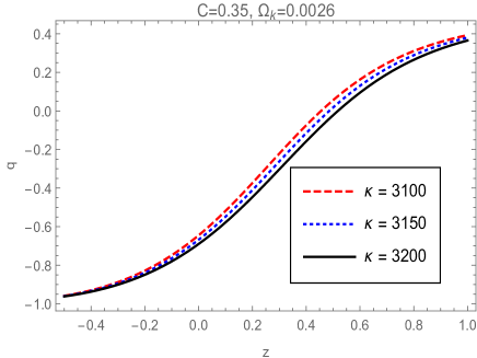
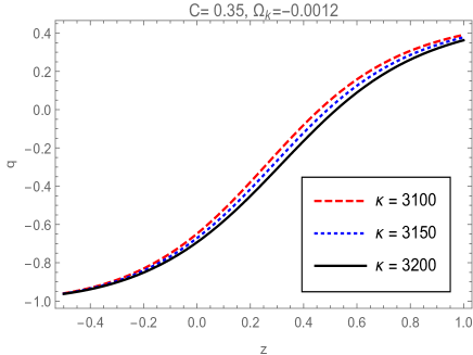
Figure 1: The evolution trajectories of deceleration parameter $q$ verses redshift $z$ for $C=0.35$ and different values of model parameter $\kappa$ with initial conditions $\Omega_{D0}$= $0.70$ and $H_{0}=67.9$. The left panel has been plotted for an open Universe with $\Omega_{K}$= $0.0026$ and the right one has been plotted for a closed Universe with $\Omega_{K}$= $-0.0012$.

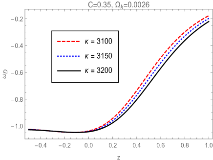
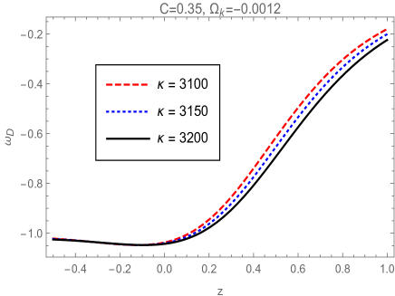
Figure 2: Behavior of EoS parameter $\omega_{D}$ versus redshift $z$ for $C=0.35$ and different values of model parameter $\kappa$ with initial conditions $\Omega_{D0}$= $0.70$ and $H_{0}=67.9$ for open Universe $\Omega_{K}$= $0.0026$ (left panel) and closed Universe $\Omega_{K}$= $-0.0012$ (right panel).

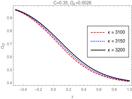
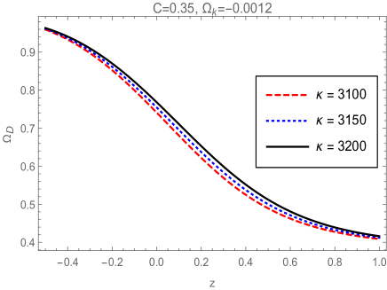
Figure 3: Behavior of density parameter $\Omega_{D}$ versus redshift $z$ for an open (left panel) and a closed (right panel) Universe for $C=0.35$ and different values of model parameter $\kappa$ with initial conditions $\Omega_{D0}$= $0.70$ and $H_{0}=67.9$.

The behavior of deceleration parameter $q$ for as a function of redshift $z$, can be obtained by examining Eq. (14) which is solved numerically by taking the initial conditions stated above. The numerical solution of $q$ is depicted in Fig. (1). We have taken different observationally best-fitted values of KHDE model parameter $\kappa=3100,\,3150$ and $3200$ and $C=0.35$ for an open Universe $\Omega_{K0}$= $0.0026$ (left panel) and close Universe $\Omega_{K0}$= $-0.012$ (right panel). We observe that the evolution of both closed as well as open Universe models from early decelerating to late-time accelerating phase of expansion occurs at transition redshift $z_{tr}$ where $q(z_{tr})=0$. The transition redshift for the present model is obtained as, $z_{tr}\approx 0.5$ as required from observations.

In order to study the nature of the EoS parameter of KHDE and specifically to investigate whether it is influenced by $\kappa$ and $\Omega_{K}$ parameters, we plot $\omega_{D}$ against redshift in Fig. (2) for different values of $\kappa$ parameter and for open (left panel) and closed (right panel) Universe models. As we can see, for different values of $\kappa$ parameter, the evolution of $\omega_{D}$ and its prevailing value $\omega_{D}(z=0)\equiv\omega_{D0}$ tend to assume more moderate values. Interestingly, for $z>0$ the EoS parameter of DE lies completely within the quintessence region. As the Universe evolves to redshift $z\leq 0$, the phantom divide ($w_{DE}=-1$) is crossed at a certain value of redshift. This value of the redshift depends on the model parameters of KHDE model. Therefore, in the framework of present model, it is possible for the EoS of KHDE to cross to the phantom regime, contrary to the case of standard HDE.

In Fig. (3) we depict the behavior of DE density parameter $\Omega_{D}$ during the evolution of an open (left panel) and a closed (right panel) Universe for different values of the Kaniadakis parameter $\kappa$. Since we witnessed the general thermal history of the Universe through the classification of matter and radiation dominated eras, the transition from matter to DE domination complies with the required scenario of structure formation of the Universe. It is remarkable that for more transparency we should extend the evolution of the Universe to the distant futurity, from where we can observe the outcomes of cosmic evolution in complete DE domination as expected. It is also noteworthy that in comparison to the flat KHDE model, where the phantom regime was not obtained, the incorporation of spatial curvature can drive the Universe into the phantom region, which can be an interesting subject of research and discussion in the future.

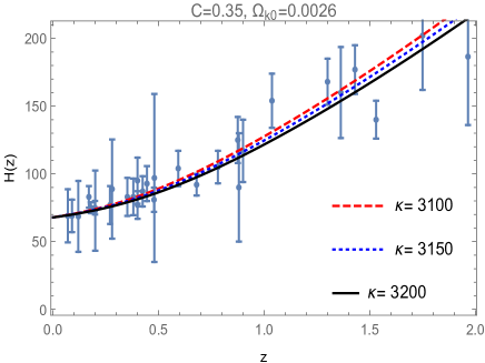
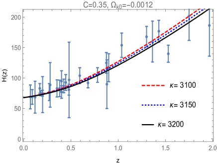
Figure 4: The evolution of $H(z)$ versus redshift $z$ with error bars for $C=0.35$ and different values of model parameter $\kappa$ with initial conditions $\Omega_{D0}$= $0.70$ and $H_{0}=67.9$ for open Universe $\Omega_{K}$= $0.0026$ (left panel) and closed Universe $\Omega_{K}$= $-0.0012$ (right panel). In this plot, the dots correspond to the 30 $H(z)$ data points

.

4 Observational data analysis

This section deals with the most advanced cosmological investigations of KHDE model. We have explained the datasets considered in our analysis in-brief, specifically, the current data of Hubble parameter has been achieved through the CC (cosmic chronometer) mode and Type Ia Supernova (SNIa).

4.1 Observational Hubble Data (OHD)

We take Hubble datasets $H(z)$ from table 4 of Ref. [56], which contains 30 $H(z)$ observational dataset limits spanning the redshift interval of $0.07\leq z\leq 1.965$. These uncorrelated data can be obtained by the cosmic chronometric (CC) technique. The purpose of taking these set of data lies in the case that the OHD dataset acquired of the CC method is individualistic. The CC data of passively evolving Universes depends on the method of distinct dating of galaxies. The evolution of $H(z)$ (Hubble parameter) for our KHDE model has been shown in Fig. (4), for both closed and open Universes, and compared with the newest 30 points of $H(z)$ data [56]. We observe that the present KHDE model is fully compatible with the OHD dataset at variance with the redshift parameter.

4.2 Distance modulus $\mu$

To examine the cosmological models, the datasets extracted from the SNIa are very beneficial particularly as a primary evidence for accelerated Universe. Therefore, we have further used the distance modulus dataset sample of 580 scores of Union 2.1 combined with SNIa [57], besides the CC data. To investigate the evolution of the Universe, there is a prominent observational tool namely the redshift-luminosity distance relation [58]. Due to the expansion of the universe, the light reaching out towards a distant luminescent body becomes redshifted and we can get the equation for the luminosity distance (DL) in terms of $z$. With help of luminosity distance, we can obtain the flux of a source, which is presented as

$$D_{L}=a_{0}r(z+1),$$ (17)

here $r$ denotes the radial coordinate of the source. Copeland et al.[59] have formulated DL as given below

$$D_{L}=\frac{c(1+z)}{H_{0}}\int_{0}^{z}\frac{dz}{h(z)},\quad h(z)=\frac{H}{H_{0}}.$$ (18)

The distance modulus $\mu$ is then obtained as [59]

$$\mu=25+5\log_{10}\left(\frac{D_{L}}{M_{pc}}\right).$$ (19)

From Eq. (18), one gets the following expression for distance modulus

$$\mu=25+5\log_{10}\left[\frac{c(1+z)}{H_{0}}\int_{0}^{z}\frac{dz}{h(z)}\right].$$ (20)

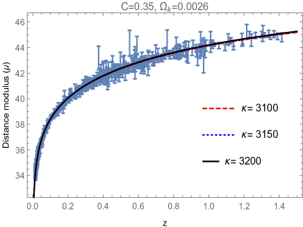
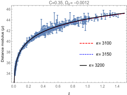
Figure 5: Evolution of Luminosity Distance versus redshift $z$ for $C=0.35$ and different values of model parameter $\kappa$ with initial conditions $\Omega_{D0}$= $0.70$ and $H_{0}=67.9$ for open Universe $\Omega_{K}$= $0.0026$ (left panel) and closed Universe $\Omega_{K}$=$-0.0012$ (right panel).

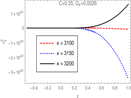
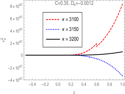
Figure 6: The behavior of $v_{s}^{2}$ against redshift $z$ for $C=0.35$ and different values of model parameter $\kappa$ with initial conditions $\Omega_{D0}$= $0.70$ and $H_{0}=67.9$ for open Universe $\Omega_{K}$= $0.0026$ (left panel) and closed Universe $\Omega_{K}$= $-0.0012$ (right panel).

Figure (5) shows the most suitable period of distance modulus $\mu$(z) in terms of $z$ for KHDE model combining the 580 scores of Union 2.1 [57] with SNIa data. This figure displays the error graph for KHDE model presented in solid line by applying 580 scores of Union 2.1 combined with SNIa datasets. Also from this figure one could easily witness the moderate reflection of KHDE model on the observed values of distance modulus $\mu$ for every data point, which indeed justifies our model.

5 Stability

The present section deals with examining classical stability of KHDE model through the squared speed of sound ($v_{s}^{2}$) for a closed as well as open FRW Universe. The squared speed of sound is given as  [60, 61]

$$v_{s}^{2}=\frac{dp_{D}}{d\rho_{D}}=\frac{\rho_{D}}{\dot{\rho}_{D}}\dot{\omega}_{D}+\omega_{D}.$$ (21)

In figure (6), we plotted the behavior of squared speed of sound ($v_{s}^{2}$) against redshift using different values of $\kappa$ parameter. As we see for some values of Kaniadakis parameter namely, $\kappa=3150$, we have $v_{s}^{2}<0$ and thus, KHDE model is not stable in both open and closed Universe models, see the blue dotted curve. However, for other values of $\kappa$ parameter $v_{s}^{2}>0$ and the KHDE model is stable for late-time, see the black solid and red dashed curves. Hence the condition on classical stability of the model puts limit on the allowed values of Kaniadakis parameter.

6 Conclusions

In this research, we have examined KHDE model in the non-flat universe which is dependent on two model parameters $C$ and $\kappa$. While estimating these model parameters we have also used the dataset samples of distance modulus of 580 scores of Union 2.1 combining SNIa along with the $30$ CC data points of $H(z)$ analyses. Besides, we have reconstructed the evolving behavior of $q(z)$, $\omega_{D}$ and $\Omega_{D}$ for the existing model, while working on the fittest values of $C$ and $\kappa$.

Proceeding to the detailed investigation, we showed that the classification of DE and matter dominated eras through the supporting diagrams can explain the Universe’s thermal history. Furthermore, we examined the effect of the Kanadakis parameter $\kappa$, as well as of the curvature density parameter at present, on the EoS parameter of DE. As we observed, the EoS parameter of DE prevails to the quintessence region, crossing the phantom-divide has been realized at present, namely KHDE favors the phantom region. However, the most attractive characteristic is that comparing to the flat case, where the phantom regime was not obtained, the incorporation of curvature leads the Universe to the phantom regime. This is an advantage since one expects that only small deviations from standard entropy could be one of the cases

It is however normal to develop the present study with the extension of other data from BAO (Baryon Acoustic Oscillation), SNIa, and CMB (Cosmic microwave background) probes in order to restrain the new parameters more accurately. Work along this line is in progress and further results on this topic will be reported in forthcoming researches.

References

- [1] J. W. Gibbs, “Elementary principles in statistical mechanics: 1902,” New York: Charles Scribner’s Sons, 1960.
- [2] G. Kaniadakis, “Non-linear kinetics underlying generalized statistics,” Physica A: Statistical mechanics and its applications, vol. 296, no. 3-4, pp. 405–425, 2001.
- [3] G. Kaniadakis, “Statistical mechanics in the context of special relativity,” Physical review E, vol. 66, no. 5, p. 056125, 2002.
- [4] M. Masi, “A step beyond tsallis and rényi entropies,” Physics Letters A, vol. 338, no. 3-5, pp. 217–224, 2005.
- [5] C. Tsallis and L. J. Cirto, “Black hole thermodynamical entropy,” The European Physical Journal C, vol. 73, no. 7, p. 2487, 2013.
- [6] H. Moradpour, “Implications, consequences and interpretations of generalized entropy in the cosmological setups,” Int. J. Theor. Phys., vol. 55, no. 9, pp. 4176–4184, 2016.
- [7] R. C. Nunes, E. M. Barboza, Jr., E. M. C. Abreu, and J. A. Neto, “Probing the cosmological viability of non-gaussian statistics,” JCAP, vol. 08, p. 051, 2016.
- [8] N. Komatsu, “Cosmological model from the holographic equipartition law with a modified Rényi entropy,” Eur. Phys. J. C, vol. 77, no. 4, p. 229, 2017.
- [9] H. Moradpour, A. Bonilla, E. M. C. Abreu, and J. A. Neto, “Accelerated cosmos in a nonextensive setup,” Phys. Rev. D, vol. 96, no. 12, p. 123504, 2017.
- [10] E. M. C. Abreu, J. A. Neto, A. C. R. Mendes, A. Bonilla, and R. M. de Paula, “Tsallis’ entropy, modified Newtonian accelerations and the Tully-Fisher relation,” EPL, vol. 124, no. 3, p. 30005, 2018.
- [11] M. Tavayef, A. Sheykhi, K. Bamba, and H. Moradpour, “Tsallis holographic dark energy,” Physics Letters B, vol. 781, pp. 195–200, 2018.
- [12] A. S. Jahromi, S. Moosavi, H. Moradpour, J. M. Graça, I. Lobo, I. Salako, and A. Jawad, “Generalized entropy formalism and a new holographic dark energy model,” Physics Letters B, vol. 780, pp. 21–24, 2018.
- [13] U. K. Sharma, G. Varshney, and V. C. Dubey, “Barrow agegraphic dark energy,” Int. J. Mod. Phys. D, vol. 30, no. 03, p. 2150021, 2021.
- [14] H. Moradpour, S. Moosavi, I. Lobo, J. M. Graça, A. Jawad, and I. Salako, “Thermodynamic approach to holographic dark energy and the rényi entropy,” The European Physical Journal C, vol. 78, no. 10, p. 829, 2018.
- [15] S. Srivastava and U. K. Sharma, “Barrow holographic dark energy with Hubble horizon as IR cutoff,” Int. J. Geom. Meth. Mod. Phys., vol. 18, no. 01, p. 2150014, 2021.
- [16] T. S. Biró and V. G. Czinner, “A q-parameter bound for particle spectra based on black hole thermodynamics with rényi entropy,” Physics Letters B, vol. 726, no. 4-5, pp. 861–865, 2013.
- [17] S. Ghaffari, A. Ziaie, H. Moradpour, F. Asghariyan, F. Feleppa, and M. Tavayef, “Black hole thermodynamics in sharma–mittal generalized entropy formalism,” General Relativity and Gravitation, vol. 51, no. 7, pp. 1–11, 2019.
- [18] S. Ghaffari, A. Ziaie, V. Bezerra, and H. Moradpour, “Inflation in the rényi cosmology,” Modern Physics Letters A, vol. 35, no. 01, p. 1950341, 2020.
- [19] H. Moradpour, A. H. Ziaie, S. Ghaffari, and F. Feleppa, “The generalized and extended uncertainty principles and their implications on the Jeans mass,” Mon. Not. Roy. Astron. Soc., vol. 488, no. 1, pp. L69–L74, 2019.
- [20] H. Moradpour, A. Sheykhi, C. Corda, and I. G. Salako, “Implications of the generalized entropy formalisms on the Newtonian gravity and dynamics,” Phys. Lett. B, vol. 783, pp. 82–85, 2018.
- [21] H. Moradpour, C. Corda, A. H. Ziaie, and S. Ghaffari, “The extended uncertainty principle inspires the Rényi entropy,” EPL, vol. 127, no. 6, p. 60006, 2019.
- [22] J. D. Barrow, “The Area of a Rough Black Hole,” Phys. Lett. B, vol. 808, p. 135643, 2020.
- [23] M. Srednicki, “Entropy and area,” Phys. Rev. Lett., vol. 71, pp. 666–669, 1993.
- [24] S. Das and S. Shankaranarayanan, “Where are the black hole entropy degrees of freedom?,” Class. Quant. Grav., vol. 24, pp. 5299–5306, 2007.
- [25] D. Pavon, “On the degrees of freedom of a black hole,” arXiv preprint arXiv:2001.05716, 2020.
- [26] M. Li, “A model of holographic dark energy,” Physics Letters B, vol. 603, no. 1-2, pp. 1–5, 2004.
- [27] Y. S. Myung, “Instability of holographic dark energy models,” Phys. Lett. B, vol. 652, pp. 223–227, 2007.
- [28] S. A. Hayward, “Unified first law of black hole dynamics and relativistic thermodynamics,” Class. Quant. Grav., vol. 15, pp. 3147–3162, 1998.
- [29] S. A. Hayward, S. Mukohyama, and M. C. Ashworth, “Dynamic black hole entropy,” Phys. Lett. A, vol. 256, pp. 347–350, 1999.
- [30] D. Bak and S.-J. Rey, “Cosmic holography+,” Classical and Quantum Gravity, vol. 17, no. 15, p. L83, 2000.
- [31] R.-G. Cai and S. P. Kim, “First law of thermodynamics and friedmann equations of friedmann-robertson-walker universe,” Journal of High Energy Physics, vol. 2005, no. 02, p. 050, 2005.
- [32] M. Akbar and R.-G. Cai, “Thermodynamic behavior of the friedmann equation at the apparent horizon of the frw universe,” Physical Review D, vol. 75, no. 8, p. 084003, 2007.
- [33] R.-G. Cai, L.-M. Cao, and Y.-P. Hu, “Hawking radiation of an apparent horizon in a frw universe,” Classical and Quantum Gravity, vol. 26, no. 15, p. 155018, 2009.
- [34] Q. Huang, H. Huang, J. Chen, L. Zhang, and F. Tu, “Stability analysis of a tsallis holographic dark energy model,” Classical and Quantum Gravity, vol. 36, no. 17, p. 175001, 2019.
- [35] S. H. Shekh, P. H. R. S. Moraes, and P. K. Sahoo, “Physical acceptability of the renyi, tsallis and sharma-mittal holographic dark energy models in the f(t,b) gravity under hubble’s cutoff,” Universe, vol. 7, no. 3, 2021.
- [36] M. Zubair and L. R. Durrani, “Exploring tsallis holographic dark energy scenario in f(r,t) gravity,” Chinese Journal of Physics, vol. 69, pp. 153–171, 2021.
- [37] S. Bhattacharjee, “Growth rate and configurational entropy in tsallis holographic dark energy,” The European Physical Journal C, vol. 81, Mar 2021.
- [38] M. Nauenberg, “Critique of q-entropy for thermal statistics,” Physical Review E, vol. 67, no. 3, p. 036114, 2003.
- [39] L. G. Moyano, F. Baldovin, and C. Tsallis, “Zeroth principle of thermodynamics in aging quasistationary states,” arXiv preprint cond-mat/0305091, 2003.
- [40] C. Tsallis, “Comment on “critique of q-entropy for thermal statistics”,” Physical Review E, vol. 69, no. 3, p. 038101, 2004.
- [41] M. Nauenberg, “Reply to “comment on ‘critique of q-entropy for thermal statistics’”,” Physical Review E, vol. 69, no. 3, p. 038102, 2004.
- [42] W. Li, Q. A. Wang, L. Nivanen, and A. Le Méhauté, “On different q-systems in nonextensive thermostatistics,” The European Physical Journal B-Condensed Matter and Complex Systems, vol. 48, no. 1, pp. 95–100, 2005.
- [43] S. Abe, “Temperature of nonextensive systems: Tsallis entropy as clausius entropy,” Physica A: Statistical Mechanics and its Applications, vol. 368, no. 2, pp. 430–434, 2006.
- [44] T. Biró and P. Ván, “Zeroth law compatibility of nonadditive thermodynamics,” Physical Review E, vol. 83, no. 6, p. 061147, 2011.
- [45] T. Biró and P. Ván, “Publisher’s note: Zeroth law compatibility of nonadditive thermodynamics [phys. rev. e 83, 061147 (2011)],” Physical Review E, vol. 84, no. 1, p. 019902, 2011.
- [46] E. M. Abreu, J. A. Neto, A. C. Mendes, A. Bonilla, and R. M. de Paula, “Cosmological considerations in kaniadakis statistics,” EPL (Europhysics Letters), vol. 124, no. 3, p. 30003, 2018.
- [47] H. Moradpour, A. Ziaie, and M. K. Zangeneh, “Generalized entropies and corresponding holographic dark energy models,” The European Physical Journal C, vol. 80, no. 8, pp. 1–7, 2020.
- [48] A. Jawad and A. M. Sultan, “Cosmic Consequences of Kaniadakis and Generalized Tsallis Holographic Dark Energy Models in the Fractal Universe,” Adv. High Energy Phys., vol. 2021, p. 5519028, 2021.
- [49] S. Vagnozzi, A. Loeb, and M. Moresco, “Eppur è piatto? The Cosmic Chronometers Take on Spatial Curvature and Cosmic Concordance,” Astrophys. J., vol. 908, no. 1, p. 84, 2021.
- [50] N. Aghanim et al., “Planck 2018 results. VI. Cosmological parameters,” Astron. Astrophys., vol. 641, p. A6, 2020.
- [51] S. Vagnozzi, E. Di Valentino, S. Gariazzo, A. Melchiorri, O. Mena, and J. Silk, “Listening to the BOSS: the galaxy power spectrum take on spatial curvature and cosmic concordance,” 10 2020.
- [52] E. Di Valentino, A. Melchiorri, and J. Silk, “Investigating Cosmic Discordance,” Astrophys. J. Lett., vol. 908, no. 1, p. L9, 2021.
- [53] A. Sheykhi, “Modified friedmann equations from tsallis entropy,” Physics Letters B, vol. 785, pp. 118–126, 2018.
- [54] S. A. Hayward, S. Mukohyama, and M. Ashworth, “Dynamic black-hole entropy,” Physics Letters A, vol. 256, no. 5-6, pp. 347–350, 1999.
- [55] S. A. Hayward, “Unified first law of black-hole dynamics and relativistic thermodynamics,” Classical and Quantum Gravity, vol. 15, no. 10, p. 3147, 1998.
- [56] M. Moresco, L. Pozzetti, A. Cimatti, R. Jimenez, C. Maraston, L. Verde, D. Thomas, A. Citro, R. Tojeiro, and D. Wilkinson, “A 6% measurement of the hubble parameter at z 0.45: direct evidence of the epoch of cosmic re-acceleration,” Journal of Cosmology and Astroparticle Physics, vol. 2016, no. 05, p. 014, 2016.
- [57] N. Suzuki, D. Rubin, C. Lidman, G. Aldering, R. Amanullah, K. Barbary, L. Barrientos, J. Botyanszki, M. Brodwin, N. Connolly, et al., “The hubble space telescope cluster supernova survey. v. improving the dark-energy constraints above z¿ 1 and building an early-type-hosted supernova sample,” The Astrophysical Journal, vol. 746, no. 1, p. 85, 2012.
- [58] A. R. Liddle and D. H. Lyth, Cosmological inflation and large-scale structure. Cambridge university press, 2000.
- [59] E. Copeland, “M sami and s tsujikawa int. j. mod,” Phys. D, vol. 15, p. 1753, 2006.
- [60] E. Calabrese, R. de Putter, D. Huterer, E. V. Linder, and A. Melchiorri, “Future cmb constraints on early, cold, or stressed dark energy,” Physical Review D, vol. 83, no. 2, p. 023011, 2011.
- [61] S. Vagnozzi, L. Visinelli, O. Mena, and D. F. Mota, “Do we have any hope of detecting scattering between dark energy and baryons through cosmology?,” Monthly Notices of the Royal Astronomical Society, vol. 493, no. 1, pp. 1139–1152, 2020.