Qualitative analysis of a mathematical model for Xylella fastidiosa epidemics.

Abstract

In Southern Italy, since 2013, there has been an ongoing Olive Quick Decline Syndrome (OQDS) outbreak, due to the bacterium Xylella fastidiosa. In a couple of previous papers, the authors have proposed a mathematical approach for identifying possible control strategies for eliminating or at least reduce the economic impact of such event. The main players involved in OQDS are represented by the insect vector, Philaenus spumarius, its host plants (olive trees and weeds) and the bacterium, X. fastidiosa. A basic mathematical model has been expressed in terms of a system of ordinary differential equations; a preliminary analysis already provided interesting results about possible control strategies within an integrated pest management framework, not requiring the removal of the productive resource represented by the olive trees. The same conjectures have been later confirmed by analyzing the impact of possible spatial heterogeneities on controlling a X. fastidiosa epidemic. These encouraging facts have stimulated a more detailed and rigorous mathematical analysis of the same system, as presented in this paper. A clear picture of the possible steady states (equilibria) and their stability properties has been outlined, within a variety of different parameter scenarios, for the original spatially homogeneous ecosystem.

The results obtained here confirm, in a mathematically rigorous way, what had been conjectured in the previous papers, i.e. that the removal of a suitable amount of weed biomass (reservoir of the juvenile stages of the insect vector of X. fastidiosa from olive orchards and surrounding areas is the most acceptable strategy to control the spread of the OQDS. In addition, as expected, the adoption of more resistant olive tree cultivars has been shown to be a good strategy, though less cost-effective, in controlling the pathogen.

Keywords: Xylella fastidiosa; olive trees; epidemics; mathematical model; numerical simulations; control strategies.

1 Introduction

The etiological agent of the olive quick decline syndrome (OQDS), a disease that have seriously affected the olive production in Apulia region (Italy) since 2013, is the plant pathogenic bacterium Xylella fastidiosa (Proteobacteria, Xanthomonadaceae). Once a plant is infected, bacteria multiplication within the xylem vessels can lead to the formation of a biofilm, which can occlude the xylem vessels, thus inhibiting the plant water supply. Typical symptoms are leaf scorch, dieback of twigs, branches and even of the whole plant (see e.g. [6]).

In addition to olive trees, Xylella fastidiosa can infect a large number of other plants, some of which crops of relevant economic interest, such as grapevines, almond trees, citrus plants, etc. (see e.g. [11]).

The main vector of Xylella fastidiosa in Southern Italy has been identified in the so-called meadow spittlebug, i.e., Philaenus spumarius (Hemiptera, Aphrophoridae), a xylem sap- feeding specialist (see e.g.[12]). In an olive orchard, the juvenile form (nymphs) develops on weeds or ornamental plants, in a self-produced foam for protection from predators and water loss, the adult moves to olive tree canopies at the end of the spring/early summer, where it remains until the end of the summer, before returning back to weeds for reproduction..

The scope of our research is the mathematical modelling of the dinamics of a Xylella fastidiosa epidemics within olive orchard agroecosystems. A sound mathematical model let us perform predictive analysis of the relevant components of the system, so as to suggest possible control strategies.

In previous papers ([4], [2]), motivated by the outbreak of OQDS in Southern Italy, models describing the epidemic have been presented.

In [4], a basic model was presented, based on a system of ordinary differential equations (ODEs), describing a basic spatially homogeneous ecosystem includ- ing the main three players, i.e., the insect vector, P. spumarius, the olive trees, and weeds. In the same paper only a preliminary mathematical analysis had been reported which anyhow anticipated rather encouraging results concerning satisfactory agronomic practices for the control and possible eradication of a Xylella fastidiosa epidemic on olive trees.

We have then been motivated to carry out a more detailed and rigorous mathematical analysis of the same system, which has been the scope of paper [2], and of the present paper.

While paper [2] had been devoted to explore the impact of possible spatial heterogeneities on controlling a X. fastidiosa epidemic, in the present paper we have finally succeeded in establishing a clear picture of the possible steady states (equilibria) and their stability properties, within a variety of different parameter scenarios, though for a spatially homogeneous ecosystem. The results obtained here confirm, supported by a mathematically rigorous analysis, what had been already conjectured in the previous papers, i.e. that ”the removal of a significant amount of weeds (acting as a reservoir for juvenile insects) from olive orchards and surrounding areas has resulted in the most efficient strategy to control the spread of the OQDS. In addition, as expected, the adoption of more resistant olive tree cultivars has been shown to be a good strategy, though less cost effective, in controlling the pathogen.” [4].

The theoretical mathematical analysis has been supported by a set of numerical experiments, which show in a quantitative way the role of crucial parameters of the system for possible control, with particular attention to the choice of the olive cultivar (with respect to their resistance to X. fastidiosa infections) and the weed elimination in the relevant orchards. It is worth mentioning that, in recent investigations presented in [16], the authors, by means of a cellular automaton simulator, have confirmed the relevance of the olive cultivar as a possible control strategy.

The paper is organized as follows. In Sections 2 and 3 the mathematical model is presented. In Section 4 feasible equilibria have been obtained their stability properties have been analyzed in Section 5. Finally in Section 6 numerical simulations are presented which confirm the analytical results; in the numerical simulations, the relevant parameters have been taken from [4]. The paper ends with relevant concluding remarks, in Section 7.

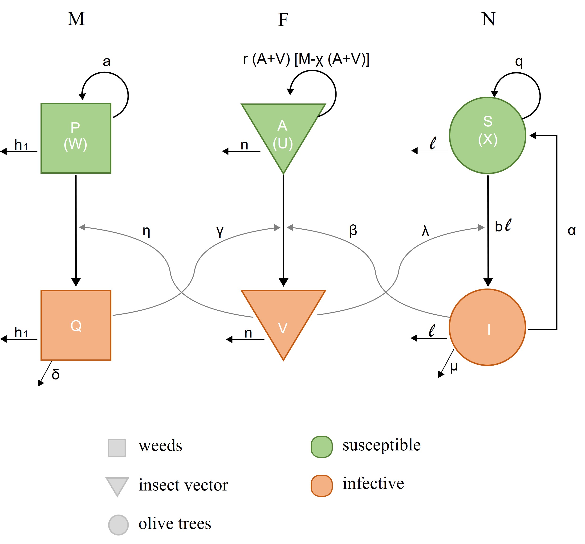
Figure 1: Diagram of interactions.

2 Building blocks of the mathematical model

As anticipated in the Introduction, we shall analyze here the same model proposed in [4], including what can be considered the most significant features of the dynamics of a real epidemic system, with respect to possible control strategies. Accordingly only the following components have been considered.

The individuals of the insect (P. Spumarius) population will be denoted by $A$ if healthy and by $V$ if infected. The populations of susceptible and infected olive trees will be respectively denoted by $S$ and $I$ (see Table 1). As a third player of the modelled ecosystem we consider the so called weeds, which collectively include all herbaceous and shrub-like plants that may constitute a reservoir for the bacterial pathogen X. fastidiosa. The number of healthy weeds will be denoted by $P,$ while $Q$ stands for the infected ones. All the parameters in the model are non-negative quantities.

2.1 The dynamics of insects

The equations describing the evolution of the two insect subpopulations are the following ones

$$\left\{\begin{array}[]{l}\displaystyle{\frac{dA}{dt}=r(A+V)(P+Q)-r\chi A(A+V)-nA}\\ \quad\quad\quad\displaystyle{-\beta\frac{I}{S+I}A-\gamma\frac{Q}{P+Q}A,}\\ \displaystyle{\frac{dV}{dt}=-nV-r\chi V(A+V)}\displaystyle{+\beta\frac{I}{S+I}A+\gamma\frac{Q}{P+Q}A.}\end{array}\right.$$ (1)

It has been taken into account the fact that bacteria are not vertically transmitted by female insects, so that the latter generate only healthy offspring, independently of their status as healthy or infected (see e.g. [1], [13], and references therein). The development of nymphs and their molting into adults, however, require weeds in the environment (either healthy or infected); this has been expressed by the dependence (here assumed to be linear) of the birth rate upon the total weed population. We may notice that the overall reproduction rate of insects is given by

$$r(A+V)[(P+Q)-\chi(A+V)],$$ (2)

where a logistic term $[(P+Q)-\chi(A+V)]$ has been introduced; this means that the total population of weeds $(P+Q)$ acts as carrying capacity for the insects; $\chi$ has been introduced as a tuning parameter with respect to available data.

Insects experience a natural mortality at a rate $n,$ which here is assumed to be a constant parameter, as a technical simplification. They may become infected by feeding on infected trees or plants. The insect infection rate is assumed to be a linear function of the relative abundances of infected biomasses (with respect to their respective total values) of both trees and weeds, via the parameters $\beta$ and $\gamma,$ respectively.

2.2 The dynamics of olive trees

For the olive trees it is better to refer to their canopies, so that we may consider pruning and regrowth. Their dynamics is described by the following two equations:

$$\left\{\begin{array}[]{l}\displaystyle{\frac{dS}{dt}=\left(q-\frac{S+I}{C}\right)S-\ell S-\lambda VS-b\ell\frac{I}{I+S}S+\alpha I,}\\ \\ \displaystyle{\frac{dI}{dt}=-\frac{S+I}{C}I+\lambda VS-\mu I-\ell I+b\ell\frac{I}{I+S}S-\alpha I.}\end{array}\right.$$ (3)

Healthy trees (canopy) $S$ are produced by regrowth (or additional planting). The production of healthy trees has been described by a logistic growth model

$$\left[q-\frac{S+I}{C}\right]S$$ (4)

where $q$ is the natural constant growth rate, and the logistic term $\displaystyle\frac{S+I}{C}$ takes into account a possible carrying capacity $C.$ Correspondingly in the second equation, concerning infected trees, a logistic term $\displaystyle\frac{S+I}{C}I$ has been included.

For trees, in view of their long survival, natural mortality has been neglected; a constant decay rate $\ell,$ due to regular pruning (or possible elimination/logging) has instead been included. Canopies of infected trees $I$ experience a disease- related extra mortality $\mu.$ A possible recovery of trees might be considered at a constant rate $\alpha.$

Trees get infected by contact with infected adult insects, or by human ac- tivities such as pruning, budding and grafting, due to the use of infected tools. As far as the incidence rate due to infected insects is concerned the following form has been assumed, after a reasoning supported by [8] (see also [5]),

$$\lambda VS.$$ (5)

The incidence rate due to human activities has been considered proportional to the relative abundance of infected trees with respect to their total mass. Given $\ell,$ the rate of contacts with tools employed for human activities, we have

$$b\ell\frac{I}{I+S}S.$$ (6)

2.3 The dynamics of weeds

The dynamics of the weeds mass is described by the following two equations:

$$\left\{\begin{array}[]{l}\displaystyle{\frac{dP}{dt}=\left(a-\frac{P}{C_{2}}\right)(P+Q)-\eta VP-h_{P}(P,Q),}\\ \\ \displaystyle{\frac{dQ}{dt}=-\frac{P+Q}{C_{2}}Q+\eta VP-\delta Q-h_{Q}(P,Q).}\end{array}\right.$$ (7)

As above, logistic growth is assumed, at a net reproduction rate $a$ and carrying capacity $C_{2};$ we assume that all weeds produce healthy ones. For the infection rate of weeds we have made the same assumptions as for the olive trees, so that the incidence rate for weeds is

$$\eta VP.$$ (8)

Disease-related mortality of weeds occurs at rate $\delta,$ while $h_{P}$ and $h_{Q}$ represent mass reduction due to human-related activities. We have assumed that they are linearly dependent on the size of the existing vegetation, i.e.:

$$h_{P}(P,Q)=h_{1}P,\quad h_{Q}(P,Q)=h_{1}Q.$$ (9)

Later $h_{1}$ (year$-1$) will be used as a control parameter for the eventual eradi- cation of the epidemic in the relevant habitat; $h_{1}=0$ will mean that weeds are subject only to their natural dynamics.

An important remark is due concerning the above model.

 Remark 1

In Systems (1) and (3), the terms

$$\frac{I}{I+S}\quad\textnormal{and}\quad\displaystyle\frac{Q}{P+Q}$$ (10)

may degenerate, i.e. their denominators may become zero. For a sound mathe- matical model, in either case we have to assume that the whole fraction is taken as zero.

Table 1: Model variables.

Symbol	Description
A	Healthy insects
V	Infected insects
U	Fraction of healthy insects
F	Total population of insects
S	Healthy olive trees
I	Infected olive trees
X	Fraction of healthy olive trees
N	Total canopy mass of olive trees
P	Healthy weeds
Q	Infected weeds
W	Fraction of healthy weeds
M	Total mass of weeds

Table 2: Model parameters.

Symbol	Description
$r$	Insects birth rate
$\chi$	Insect intraspecific competition rate
$n$	Insects mortality rate
$q$	Healthy trees (canopy) regrowth rate
$C$	Trees carrying capacity parameter
$\ell$	Elimination rate of trees by pruning or logging
$b$	Infection rate of trees by infected tools
$\mu$	Infected trees mortality rate
$\alpha$	Infected trees recovery rate
$a$	Weeds net growth rate
$C_{2}$	Weeds carrying capacity parameter
$\delta$	Weeds mortality rate
$\beta$	Insects infection rate by infected trees
$\gamma$	Insects infection rate by infected weeds
$\lambda$	Trees infection rate by infected insects
$\eta$	Weeds infection rate by infected insects
$h_{1}$	Weeds elimination rate by human intervention

3 The model with fractions

For the sake of simplicity we take all absolute populations as adimensional quantities. We will now rewrite our evolution equations in terms of total populations and their susceptible fractions (see also Table 1): the total number of insects $F=A+V,$ and the fraction of susceptibles $U=AF^{-1};$ the total canopy mass of olive trees $N=S+I$ and the fraction of susceptible mass $X=SN^{-1};$ the total weeds mass $M=P+Q$ and the fraction of susceptible mass $W=PM^{-1}.$ In terms of these variables our system becomes

$$\left\{\begin{array}[]{l}\vskip 6.0pt plus 2.0pt minus 2.0pt\displaystyle{\frac{dU}{dt}=rM(1-U)-[\beta(1-X)+\gamma(1-W)]U,}\\ \vskip 6.0pt plus 2.0pt minus 2.0pt\displaystyle{\frac{dF}{dt}=F[r(M-\chi F)-n],}\\ \vskip 6.0pt plus 2.0pt minus 2.0pt\displaystyle{\frac{dX}{dt}=X[(q+\mu-b\ell)(1-X)-\lambda(1-U)F]+\alpha(1-X),}\\ \vskip 6.0pt plus 2.0pt minus 2.0pt\displaystyle{\frac{dN}{dt}=N[qX-\ell-\frac{N}{C}-\mu(1-X)],}\\ \vskip 6.0pt plus 2.0pt minus 2.0pt\displaystyle{\frac{dW}{dt}=a(1-W)+W[\delta(1-W)-\eta(1-U)F],}\\ \vskip 6.0pt plus 2.0pt minus 2.0pt\displaystyle{\frac{dM}{dt}=M\left[a-\frac{M}{C_{2}}-\delta(1-W)-h_{1}\right].}\end{array}\right.$$ (11)

 Remark 2

As noticed above in Remark 1 this system may degenerate in case either $M$ or $F$ or $N$ becomes zero, so that it has to be complemented by the assumption that the corresponding fraction looses its meaning as such. For example, if $M=0$ then any value of $W\in[0,1]$ will make $WM=0,$ which is coherent with its biological meaning: if the total weed mass is zero, then the mass of healthy weeds is zero too.

It is not difficult to show that if System (11) is subject to initial conditions $U(0)\in(0,1),F(0)>0;X(0)\in(0,1);N(0)>0;W(0)\in(0,1),M(0)>0,$ then there exist $\bar{F},\bar{N},\bar{M}$ such that, for any time $t>0,$ $U(t)\in(0,1),0<F(t)<\bar{F};$ $X(t)\in(0,1),0<N(t)<\bar{N};$ $W(t)\in(0,1),0<M(t)<\bar{M}.$

We shall denote by $\mathcal{U}:=(0,1)\times(0,\bar{F})\times(0,1)\times(0,\bar{N})\times(0,1)\times(0,\bar{M});$ $\bar{\mathcal{U}}$ shall denote the closure of $\mathcal{U}.$ So that we may claim that $\bar{\mathcal{U}}$ is an invariant region for System (11).

Our aim here is to analyze the qualitative behaviour of System (11). First of all we may look for the possible existence of equilibria, which can be obtained by solving the following system of equations, subject to Remark 2,

$$rM(1-U)-[\beta(1-X)+\gamma(1-W)]U=0,$$ (12)

$$F[r(M-\chi F)-n]=0,$$ (13)

$$X[(q+\mu-b\ell)(1-X)-\lambda(1-U)F]+\alpha(1-X)=0,$$ (14)

$$N\left[qX-\ell-\frac{N}{C}-\mu(1-X)\right]=0,$$ (15)

$$a(1-W)+W[\delta(1-W)-\eta(1-U)F]=0,$$ (16)

$$M\left[a-\frac{M}{C_{2}}-\delta(1-W)-h_{1}\right]=0.$$ (17)

4 Equilibria

Consider first the case $a>0$ and $h_{1}=0.$

We will carry out the analysis of the possible equilibria of System (12)-(17) in terms of the value of $\lambda,$ the infection rate of olive trees by infective insects, which expresses the resistance to infection by a specific cultivar.

4.1 The disease free equilibrium

For $\lambda=0,$ Equation (14) can be rewritten as

$$X[(q+\mu-b\ell)(1-X)]+\alpha(1-X)=0,$$ (18)

which admits the solution $X_{1}=1.$

From here Equation (15) becomes

$$N\left[q-\ell-\frac{N}{C}\right]=0.$$ (19)

This admits the solution $N_{1}=C(q-\ell),$ which is biologically intuitive.

If in addition $\eta=0,$ Equation (16) becomes

$$a(1-W)+W[\delta(1-W)]=0,$$ (20)

which admits the solution $W_{1}=1.$

As a consequence Equation (17) becomes

$$M\left[a-\frac{M}{C_{2}}\right]=0,$$ (21)

which admits the solution $M_{1}=C_{2}a.$

If $\displaystyle C_{2}a>\frac{n}{r},$ then Equation (13) admits the solution

$$F_{1}=\frac{1}{\chi}\ \left[M_{1}-\frac{n}{r}\right].$$ (22)

Moreover Equation (12) becomes

$$rM(1-U)=0,$$ (23)

which admits the solution $U_{1}=1.$

To conclude, in absence of transmission, i.e. for $\lambda=\eta=0,$ if we make the trivial assumptions that $q>\ell,$ and $\displaystyle C_{2}a>\frac{n}{r},$ which are satisfied as from Table 3, it is not difficult to check that the following one is a nontrivial equilibrium of the ODE system (11)

$$E_{1}=(U_{1},F_{1},X_{1},N_{1}W_{1}M_{1}):=(1,\frac{1}{\chi}\ \left[M_{1}-\frac{n}{r}\right]1;C(q-\ell),1;C_{2}a).$$ (24)

It is clear that we may obtain the same equilibrium by imposing a priori $U=1;$ this situation is anyhow less interesting from the point of view of the stability analysis.

Table 3: Values of the model parameters. For parameters given in a range, the value before the brackets has been used for simulations, unless otherwise specified.

Symbol	Values	References
$r$	200 [37,400] year-1	[17, 20]
$\chi$	0.001, 0.01	[4]
$n$	0.98 [0.95, 0.99] year-1	[4]
$q$	0.5 [0.2, 0.7] year-1	[18]
$C$	100	[4]
$\ell$	0.01 year-1	[4]
$b$	$0.05$	[4]
$\mu$	0.9 [0.8, 1] year-1	[14, 15]
$\alpha$	0.1, 0.5 year-1	[4]
$a$	0.3 [0.1, 1.] year-1	[4]
$C_{2}$	$10\times C$	[4]
$\delta$	0.2 [0, 0.5] year-1	[15]
$h_{1}$	[0, 0.8] year-1	[4]
$\beta$	0.75 year-1	[7]
$\gamma$	0.1 [0.1, 0.5] year-1	[7]
$\lambda$	[0.2, 0.8] year-1	[3, 10]
$\eta$	0.1 [0.1, 0.6] year-1	[7]

4.2 Other equilibria

Let us now consider the case $\lambda>0,$ and look for nontrivial equilibria, by im- posing that the ecosystem is exposed to a nontrivial infective insect population, which is given by $(1-U)F>0.$ Consider first the equation for $X,$ the fraction of healthy olive tree biomass

$$X[(q+\mu-b\ell)(1-X)-\lambda(1-U)F]+\alpha(1-X)=0,$$ (25)

This can be rewritten as a second order algebraic equation

$$AX^{2}+BX+C=0,$$ (26)

with

$$A:=q+\mu-b\ell,$$ (27)

$$C:=-\alpha,$$ (28)

$$B:=\lambda(1-U)F-(A+C).$$ (29)

The solutions of (26) are given by

$$X^{*}_{\pm}=\frac{-B\pm\sqrt{B^{2}-4AC}}{2A}.$$ (30)

Since, by the parameter values taken from Table 3, it is $A>0,$ we may claim that $AC<0,$ so that $\sqrt{B^{2}-4AC}>B,$ and finally the existence of a nontrivial solution $X^{*}>0.$

We may further notice that $X^{*}<1$ iff $\sqrt{B^{2}-4AC}<2A+B,$ i.e. iff $B+A+C=\lambda(1-U)F>0.$

We have thus proven the following result.

 Proposition 1

For $\lambda>0$ and any value of the infective insect population $(1-U)F>0$, there exists a unique nontrivial equilibrium $X^{*}\in(0,1)$ for the fraction of healthy olive trees.

We may now turn to the analysis of the equilibrium equation for the total tree biomass, under the assumptions of the above proposition.

If we look for nontrivial solutions of the equilibrium equation for $N,$

$$N\left[qX-\ell-\frac{N}{C}-\mu(1-X)\right]=0,$$ (31)

it reduces to

$$qX-\ell-\frac{N}{C}-\mu(1-X)=0,$$ (32)

from which we obtain the equilibrium

$$N^{*}=C(q+\mu)\left[X^{*}-\frac{\mu+\ell}{\mu+q}\right].$$ (33)

This shows that (31) admits a solution $N^{*}>0$ iff

$$X^{*}>\frac{\mu+\ell}{\mu+q}.$$ (34)

Usually $\ell<q,$ so that we may claim that the following statement holds true.

 Corollary 1

Under the assumptions of Proposition 1, a unique nontrivial equilibrium $N^{*}>0$ exists for the total tree biomass iff

$$X^{*}\in\left(\frac{\mu+\ell}{\mu+q},1\right)\neq\emptyset.$$ (35)

Otherwise (31) admits only the trivial solution $N^{*}=0.$

 Remark 3

Notice that Condition (35 ) may apply only if the pruning rate $\ell$ is smaller than the natural growth rate $q$ of the biomass. If this condition does not hold then the olive trees will eventually disappear, independently of other conditions.

To conclude the analysis of a possible nontrivial equilibrium, let now consider the equilibrium equation for the fraction of healthy weeds

$$a(1-W)+W[\delta(1-W)-\eta(1-U)F]=0.$$ (36)

Under the assumption that $a>0,$ we may introduce the quantities

$$D:=\frac{\delta}{a},$$ (37)

$$G:=1-\frac{\delta}{a}+\frac{\eta}{a}(1-U)F,$$ (38)

$$L=-1.$$ (39)

so that Equation (36) can be rewritten in the form

$$DW^{2}+GW+L=0.$$ (40)

It admits two solutions given by

$$W^{*}_{\pm}=\frac{-G\pm\sqrt{G^{2}+4D}}{2D}.$$ (41)

It is not difficult to see that $D\in(0,1)$ (which is usually the case) implies $G>0,$ so that Equation (36) admits a unique nontrivial solution $W^{*}_{+}>0.$ We may then claim that the following statement holds true.

 Proposition 2

Under the assumptions of Proposition 1, if further $\displaystyle\frac{\delta}{a}\in(0,1),$ there exists a unique nontrivial equilibrium solution for the fraction of healthy weeds, given by

$$W^{*}=\frac{-G+\sqrt{G^{2}+4D}}{2D}.$$ (42)

We may notice that $\displaystyle 1+\frac{\eta}{a}(1-U)F>1$ is equivalent to $D+G>1,$ and this is equivalent to state that $W^{*}<1.$ Altogether we may then state that, under the assumptions of Proposition 2 we have $W^{*}\in(0,1).$

For the total weed mass the equilibrium equation is

$$M\left[a-\frac{M}{C_{2}}-\delta(1-W)\right]=0.$$ (43)

As from the analysis of the equilibrium $E_{1},$ we obtain that the nontrivial solution of Equation (43) is given by

$$M=M^{*}:=C_{2}[a-\delta(1-W^{*})]\geq C_{2}(a-\delta).$$ (44)

Given the values of the parameters, as from Table 3, we may state that

$$M^{*}>\frac{n}{r}.$$ (45)

Under this condition, Equation (13) admits the nontrivial solution

$$F=F^{*}:=\frac{1}{\chi}\left[M^{*}-\frac{n}{r}\right].$$ (46)

Finally we can identify the nontrivial solution of Equation (12) in the fol- lowing form

$$U^{*}=M^{*}\left[M^{*}+\frac{\beta}{r}(1-X^{*})+\frac{\gamma}{r}(1-W^{*})\right]^{-1},$$ (47)

All the above leads to a nontrivial equilibrium

$$E_{2}=(U^{*},F^{*},X^{*},N^{*},W^{*},M^{*})\in\mathcal{U}.$$ (48)

We may recollect all the above analysis in the following statement.

 Proposition 3

Under the assumption that $\displaystyle a>\delta>0,C_{2}[a-\delta]>\frac{n}{r},$ and $\ell<q,$ a nontrivial equilibrium $E_{2}=(U_{2},F_{2},X_{2},N_{2},W_{2},M_{2})$ may exist for System (11) in the open domain $\mathcal{U},$ provided Condition (35 ) is satisfied. Otherwise this equilibrium degenerates into $E_{3}=(U_{3},F_{3},X_{3},N_{3},W_{3},M_{3})$ with

$$U_{3}\in(0,1),F_{3}=\frac{1}{\chi}\left(M_{3}-\frac{n}{r}\right),X_{3}\in\left(0,\frac{\mu+\ell}{\mu+q}\right),N_{3}=0,W_{3}\in(0,1),M_{3}>\frac{n}{r}.$$ (49)

4.3 The role of $\lambda$

From an agronomic point of view, it is interesting to discuss about the dependence of the possible equilibrium $X^{*},N^{*}$ upon $\lambda$ (in a similar way one might think about the role of $\eta$ too, but this is practically impossible to control by usual agronomic practices, since $\eta$ represents the resistance of weeds to contagion). Up to now we have noticed that for $\lambda=0$ - absence of contagion to olive trees - $X^{*}=1$ and $N^{*}=C(q-\ell),$ as in the equilibrium $E_{1}.$

The role of $\lambda$ in the case $\lambda>0$ is in general more difficult to analyze. But if we restrict ourselves to the case $\alpha=b=0,$ (26 ) simply becomes

$$AX^{2}+BX=0,$$ (50)

with $A=q+\mu,$ $B=\lambda(1-U)F-A,$ and $C=0.$

This equation admits, in addition to the trivial solution, the nontrivial solution

$$X^{*}=\frac{-B}{A}$$ (51)

i.e.

$$X^{*}=1-\frac{\lambda}{q+\mu}(1-U)F$$ (52)

which finally becomes

$$X^{*}=1-\frac{\lambda}{q+\mu}(1-U^{*})F^{*},$$ (53)

if we take the corresponding equilibrium values for $U$ and $F.$

This expression shows that the value of $X^{*}$ decreases as $\lambda$ increases, as it might be conjectured.

Let us investigate the impact of this result on the total olive tree biomass.

For the equilibrium $E_{2},$ the equilibrium value $N_{2}$ satisfies Equation (33) that we report here

$$N_{2}=C(q+\mu)\left[X_{2}-\frac{\mu+\ell}{\mu+q}\right].$$ (54)

If we impose that $N_{2}>0,$ by Equation (53 ) we have to impose

$$N_{2}=C(q+\mu)\left[X_{2}-\frac{\mu+\ell}{\mu+q}\right]=C\left[q-\ell-\lambda(1-U_{2})F_{2}\right]>0$$ (55)

which requires

$$\lambda<\frac{q-\ell}{(1-U_{2})F_{2}}.$$ (56)

On the other hand the equilibrium $E_{3}$ corresponds to the case in which $\displaystyle X_{3}<\frac{\mu+\ell}{\mu+q}$ i.e., by Equation (53),

$$\lambda>\frac{q-\ell}{(1-U_{2})F_{2}}.$$ (57)

These two inequalities (56) and (57) shed some light on the role of $\lambda$ in case of an epidemic, which means a nontrivial value of the infective insect population $(1-U^{*})F^{*},$ at equilibrium: for a sufficiently small $\lambda$ we may have the equilibrium $E_{2},$ i.e. the coexistence of a nontrivial olive tree biomass. This is not possible for sufficiently large values of $\lambda,$ in which case only the equilibrium $E_{3}$ is feasible, which means extinction of the olive tree biomass.

Actually a rigorous reasoning should take into account that the quantity $(1-U^{*})F^{*}$ may depend itself upon $\lambda.$

Anyhow, the above discussion has been confirmed by the numerical simulations (see Figures 4, 8 ): the choice of more resistant cultivar may lead to coexistence.

This is a practice already implemented in Southern Italy. In an optimal control problem, it has to be compared with quality and yield of more resistant cultivar, with respect to less resistant ones (see Section 7 for the concluding remarks).

In the following we shall investigate a different practice, which does not impose change of the olive tree cultivar, by acting instead on the agronomic practice of eliminating (or at least significantly reduce ) weeds in the relevant orchards.

4.4 The case $h_{1}>a$

Let us then analyze the case $a>0,$ with $h_{1}>a,$ according to which the weed mass cannot increase, and eventually dies out.

In fact, under this assumption, the only feasible solution of Equation (17) is the trivial one $M_{4}=0.$ As a consequence, from Equation (13), the only possible equilibrium for $F$ is the trivial one $F_{4}=0.$ By taking into account Remark 2, this implies that any values $W_{4}\in[0,1]$ and $U_{4}\in[0,1]$ are admissible, hence irrelevant for further analysis. Moreover, from Equation (14),$X_{4}=1$ so that, from Equation (15), we obtain $N_{4}=C(q-\ell).$

We may then conclude with the following proposition.

 Proposition 4

Under the assumption that $a>0,$ $\ell<q$ and $h_{1}>a,$ System (11) admits the following equilibrium

$$E_{4}=(U,0,1,C(q-\ell),W,0),$$ (58)

for irrelevant values of $U$ and $W,$ which stay anyway bounded in $[0,1].$

In synthesis, the equilibrium $E_{1}$ corresponds to a disease free ecosystem; equilibrium $E_{2}$ corresponds to coexistence of a nontrivial olive tree biomass and infective insects, which we may conjecture is possible only for a sufficiently small value of $\lambda,$ i.e. for more resistant olive tree cultivars; the equilibrium $E_{2}$ may degenerate into $E_{3}$ for a sufficiently large value of $\lambda,$ i.e. for less resistant olive cultivar. Finally the equilibrium $E_{4}$ corresponds to the eradication of the insect population, induced by the eventual eradication of the weed biomass.

5 Stability

5.1 Stability of the equilibria $E_{2}$ and $E_{3}$

We shall consider first the case of the existence of a nontrivial equilibrium $E_{2}=(U_{2},F_{2},X_{2},N_{2},W_{2},M_{2})$ for System (11) in the open domain $\mathcal{U}.$

We remind here that $X_{2}$ denotes the positive solution of the equation

$$AX^{2}+BX+C=0,$$ (59)

with

$$A:=q+\mu-b\ell,$$ (60)

$$C:=-\alpha,$$ (61)

and

$$B:=\lambda(1-U_{2})F_{2}-(A+C).$$ (62)

We shall denote the negative solution of (59) by $X^{-}_{2}.$

On the other hand we denote by $W_{2}$ the positive solution of the equation

$$DW^{2}+GW+L=0,$$ (63)

where

$$D:=\frac{\delta}{a},$$ (64)

$$G:=1-\frac{\delta}{a}+\frac{\eta}{a}(1-U_{2})F_{2},$$ (65)

$$L=-1.$$ (66)

We shall denote the negative solution of (63) by $W_{2}^{-}.$

Let us then introduce the functions

$$\Lambda(X):=A(X-X_{2}^{-}),\quad\textnormal{for}\quad X\in[0,1],$$ (67)

and

$$\Gamma(X):=D(W-W_{2}^{-}),\quad\textnormal{for}\quad W\in[0,1].$$ (68)

It is clear that $\Lambda(X)>0,$ for any $X\in[0,1],$ and $\Gamma(W)>0,$ for any $W\in[0,1].$

From now on we shall denote ${\bf Z}(t):=(U(t),F(t),X(t),N(t),W(t),M(t))^{T}.$

By centering System (11) with respect to the coordinates of $E_{2},$ we obtain

$$\frac{d}{d\,t}{\bf Z}(t)={\bf f}({\bf Z}(t)),$$ (69)

for

$${\bf f}({\bf Z})=\left(\begin{array}[]{c}\displaystyle-r\frac{M_{2}}{U_{2}}(U-U_{2})\vspace{0.2cm}\\ \displaystyle-r\chi F(F-F_{2})\vspace{0.2cm}\\ \displaystyle-\Lambda(X)(X-X_{2})\vspace{0.2cm}\\ \displaystyle-\frac{N}{C}(N-N_{2})\vspace{0.2cm}\\ \displaystyle-a\Gamma(W)(W-W_{2})\vspace{0.2cm}\\ \displaystyle a\left\{M\left[-\frac{M-M_{2}}{aC_{2}}+\frac{\delta}{a}(W-W_{2})\right]\right\}\end{array}\right),\quad{\bf Z}\in\mathcal{U}.$$ (70)

Consider the function

$$g(y)=y-1-\ln y,\quad y\in(0,+\infty).$$ (71)

It is clear that $g\in C^{1}((0,+\infty))$ and it is such that $g(y)\geq 0,$ for all $y\in(0,+\infty),$ and $g(y)=0$ iff $y=1.$

Moreover $\displaystyle g^{\prime}(y)=1-\frac{1}{y},$ so that $g^{\prime}(y)<0$ for $y\in(0,1),$ $g^{\prime}(y)>0$ for $y\in(1,+\infty),$ and $g^{\prime}(y)=0$ iff $y=1.$

In order to analyze the stability of the equilibrium $E_{2},$ we take as Lyapunov function

$$\begin{array}[]{lll}V({\bf Z})&:=&\displaystyle\frac{1}{2r}[\alpha_{U}(U-U_{2})^{2}+\beta_{F}(F-F_{2})^{2}]\vspace{0.2cm}\\ &&\displaystyle+\frac{1}{2}[\alpha_{X}(X-X_{2})^{2}+\beta_{N}(N-N_{2})^{2}]\vspace{0.2cm}\\ &&\displaystyle+\frac{1}{a}\left[\alpha_{W}g\left(\frac{W}{W_{2}}\right)+\beta_{M}g\left(\frac{M}{M_{2}}\right)\right],\end{array}$$ (72)

where $\alpha_{U},\alpha_{X},\alpha_{W}$ and $\beta_{F},\beta_{N},\beta_{M}$ are positive constants to be suitably chosen.

As a consequence of the definition, and the cited properties of the function $g,$ it is $V\in C^{1}(\mathcal{U})$ and

$$V({\bf Z})\geq 0\quad\textnormal{for all}\quad{\bf Z}\in\mathcal{U},$$ (73)

$$V({\bf Z})=0\quad\textnormal{iff}\quad{\bf Z}=E_{2}.$$ (74)

Moreover the derivative of $V$ along the trajectories of System (69 ) is given by

$$\begin{array}[]{lll}&&DV({\bf Z}(t)):=\displaystyle\mbox{grad}V({\bf Z}(t))\cdot\frac{d}{dt}{\bf Z}(t)=\mbox{grad}V({\bf Z}(t))\cdot{\bf f}({\bf Z}(t))=\vspace{0.2cm}\\ &&\displaystyle-\left[\alpha_{U}\frac{M_{2}}{U_{2}}(U(t)-U_{2})^{2}+\beta_{F}\chi F(t)(F(t)-F_{2})^{2}\right]+\vspace{0.2cm}\\ &&\displaystyle-\left[\alpha_{X}\Lambda(X(t))(X(t)-X_{2})^{2}+\beta_{N}\frac{N(t)}{aC}(N(t)-N_{2})^{2}\right]+\vspace{0.2cm}\\ &&\displaystyle+\left\{-\alpha_{W}\left(\frac{\Gamma(W(t))}{W(t)W_{2}}\right)(W(t)-W_{2})^{2}+\right.\vspace{0.2cm}\\ &&\displaystyle\left.-\beta_{M}\frac{1}{aC_{2}M_{2}}(M(t)-M_{2})^{2}+\beta_{M}\left(\frac{\delta}{aM_{2}}\right)(M(t)-M_{2})(W(t)-W_{2})\right\}.\end{array}$$ (75)

The term within $\{...\}$ in the above expression can be written as the following quadratic form

$$(W(t)-W_{2},M(t)-M_{2})\left(\begin{array}[]{cc}\displaystyle-\alpha_{W}\frac{\Gamma(W(t))}{W(t)W_{2}}&\displaystyle\frac{1}{2}\frac{\beta_{M}}{M_{2}}\frac{\delta}{a}\vspace{0.2cm}\\ \displaystyle\frac{1}{2}\frac{\beta_{M}}{M_{2}}\frac{\delta}{a}&\displaystyle-\frac{\beta_{M}}{M_{2}aC_{2}}\end{array}\right)\left(\begin{array}[]{c}W(t)-W_{2}\vspace{0.2cm}\\ M(t)-M_{2}\end{array}\right)$$ (76)

associated with the real symmetric matrix

$$Q=\left(\begin{array}[]{cc}\displaystyle-\alpha_{W}\frac{\Gamma(W)}{WW_{2}}&\displaystyle\frac{1}{2}\frac{\beta_{M}}{M_{2}}\frac{\delta}{a}\vspace{0.2cm}\\ \displaystyle\frac{1}{2}\frac{\beta_{M}}{M_{2}}\frac{\delta}{a}&\displaystyle-\frac{\beta_{M}}{M^{*}aC_{2}}\end{array}\right).$$ (77)

Let us examine the structure of the matrix $Q.$

The trace of $Q$ is given by

$$\textnormal{tr}\,Q=-\alpha_{W}\frac{\Gamma(W)}{WW_{2}}-\frac{\beta_{M}}{M_{2}aC_{2}}.$$ (78)

Since both $\alpha_{W}$ and $\beta_{M}$ are positive constants, it is clear that

$$\textnormal{tr}\,Q<0.$$ (79)

The determinant of $Q$ is given by

$$\textnormal{det}\,Q=\alpha_{W}\frac{\Gamma(W)}{WW_{2}}\frac{\beta_{M}}{M_{2}aC_{2}}-\frac{1}{4}\left(\frac{\beta_{M}}{M_{2}}\frac{\delta}{a}\right)^{2}.$$ (80)

We may choose the positive constants $\alpha_{W}$ and $\beta_{M}$ in such a way that

$$\frac{\beta_{M}}{M_{2}}\frac{\delta}{a}=1\quad\textnormal{and}\quad\alpha_{W}\frac{1}{W_{2}aC_{2}}>1,$$ (81)

so that

$$\det Q>0.$$ (82)

Conditions (79) and (82) make $Q$ a stability matrix, which implies that the quadratic form (76) is negative definite. As a consequence

$$DV({\bf Z})\leq 0\quad\textnormal{for all}\quad{\bf Z}\in\mathcal{U},$$ (83)

and

$$DV({\bf Z})=0\quad\textnormal{iff}\quad{\bf Z}=E_{2}.$$ (84)

We may then claim that the following theorem holds true.

 Theorem 1

Under the assumptions $a>0,$ $\displaystyle C_{2}(a-\delta)>\frac{n}{r},$ and $\lambda$ sufficiently small so that $\displaystyle X_{2}\in\left(\frac{\mu+\ell}{\mu+q},1\right)\neq\emptyset,$ the equilibrium $E_{2}$ is globally asymptotically stable in $\mathcal{U}.$

What can we say in case the condition $\displaystyle X_{2}>\frac{\mu+\ell}{\mu+q}$ does not hold? In this case the equilibrium $E_{2}$ degenerates into $E_{3}$ in which the total olive tree mass $N$ admits only the trivial equilibrium $N_{3}=0.$

Under these circumstances it is more convenient to split the stability analysis of $E_{3},$ by considering on one side the stability with respect to the variables $U,F,W,M,$ and on the other side the stability with respect to the variable $N.$ As from Remark 2, the stability analysis of the system with respect to the variable $X$ is irrelevant.

For the variables $U,F,W,M,$ we may take as Lyapunov function

$$\begin{array}[]{lll}V({\bf Z})&:=&\displaystyle\frac{1}{2r}[\alpha_{U}(U-U_{3})^{2}+\beta_{F}(F-F_{3})^{2}]\vspace{0.2cm}\\ &&\displaystyle+\frac{1}{a}\left[\alpha_{W}g\left(\frac{W}{W_{3}}\right)+\beta_{M}g\left(\frac{M}{M_{3}}\right)\right],\end{array}$$ (85)

where $\alpha_{U},\alpha_{W}$ and $\beta_{F},\beta_{M}$ are positive constants, and proceed as above.

For the variable $N$ we may realize that its evolution equation can be written as

$$\frac{d}{d\,t}N(t)=-\frac{N(t)}{C}(N(t)-\widehat{N}),$$ (86)

for

$$\widehat{N}=C(q+\mu)\left[X_{3}-\frac{\mu+\ell}{\mu+q}\right].$$ (87)

It is clear that, under the condition $\displaystyle X_{3}<\frac{\mu+\ell}{\mu+q},$ the quantity $\widehat{N}<0,$ so that

$$\frac{d}{d\,t}N(t)=-\frac{N(t)}{C}(N(t)-\widehat{N})\leq 0,\quad\textnormal{for}\quad N(t)\geq 0$$ (88)

and

$$\frac{d}{d\,t}N(t)=-\frac{N(t)}{C}(N(t)-\widehat{N})=0,\quad\textnormal{for}\quad N(t)=0,$$ (89)

which provides the stability of $N_{3}=0.$

We may then state the following

 Theorem 2

Under the assumptions $a>0,$ $h_{1}=0,$ $\displaystyle C_{2}(a-\delta)>\frac{n}{r},$ and $\lambda$ sufficiently large so that $\displaystyle X_{2}<\frac{\mu+\ell}{\mu+q},$ the equilibrium $E_{3}$ is globally asymptotically stable in $\mathcal{U}\cup\{N=0\}.$

5.2 Stability of the disease free equilibrium $E_{1}$

In a sense, the disease free equilibrium

$$E_{1}=\left(1,\frac{1}{\chi}\left[C_{2}a-\frac{n}{r}\right],1,C(q-\ell),1,C_{2}a\right)$$

is a particular case of the nontrivial equilibrium $E_{2},$ but for the fact that we know $U_{1}=1,$ so that $(1-U_{1})F_{1}=0.$ This implies that the quantities $X_{1}^{-}$ and $W_{1}^{-},$ respectively defined in (30) and (41), are given by $\displaystyle-\frac{\alpha}{A}$ and $\displaystyle-\frac{a}{\delta},$ respectively. As a consequence the quantities $\Lambda(X)$ and $\Gamma(W),$ defined respectively as in (67) and (68), in this case are given by

$$\Lambda(X)=A(X+\frac{\alpha}{A})$$ (90)

and

$$\Gamma(X)=\frac{\delta}{a}(W+\frac{a}{\delta}).$$ (91)

Apart from these specifications, the stability analysis of $E_{1}$ can be carried out along the same lines as for $E_{2},$ leading us to state the following

 Theorem 3

Under the assumptions $a>0,$ $\displaystyle C_{2}a>\frac{n}{r},$ and $\lambda=\eta=0,$ the equilibrium $E_{1}$ is globally asymptotically stable in $\mathcal{U}\cup\{U=1\}\cup\{X=1\}\cup\{W=1\}.$

5.3 Stability of the equilibrium $E_{4}$

We now analyze the stability of the equilibrium $E_{4}=(U,0,1,C(q-\ell),W,0),$ which is the only feasible equilibrium in $\bar{\mathcal{U}}$ in absence of weeds, i.e. for $h_{1}>a.$

Based on the discussion raised by Remark 2 in this case it is sufficient to analyze the stability of the equilibrium $E_{4}$ with respect to the only components $(F_{4}=0,X_{4}=1,N_{4}=C(q-\ell),M_{4}=0).$

In this case by denoting $\widetilde{{\bf Z}}(t):=(F(t),X(t),N(t),M(t))^{T},$ we may limit our analysis to the following system

$$\frac{d}{d\,t}\widetilde{{\bf Z}}(t)=\widetilde{{\bf f}}(\widetilde{{\bf Z}}(t)),$$ (92)

for

$$\widetilde{{\bf f}}(\widetilde{{\bf Z}})=\left(\begin{array}[]{c}\displaystyle-rF\left[\left(\frac{n}{r}-M\right)+\chi\right]\vspace{0.2cm}\\ \displaystyle-A\left(X+\frac{\alpha}{A}\right)(X-X_{4})\vspace{0.2cm}\\ \displaystyle-\frac{N}{C}(N-N_{4})\vspace{0.2cm}\\ \displaystyle-M\left[(h_{1}-a)+\frac{M}{C_{2}}+\delta(1-W)\right]\end{array}\right),\quad\widetilde{{\bf Z}}\in\widetilde{\mathcal{U}}.$$ (93)

where $\widetilde{\mathcal{U}}:=(0,\bar{F})\times(0,1)\times(0,\bar{N})\times(0,\bar{M}).$

We may remark that, due to the fact that

$$\frac{d}{d\,t}M(t)=-M(t)\left[(h_{1}-a)+\frac{M(t)}{C_{2}}+\delta(1-W(t))\right]<0,$$ (94)

for any $M(t)>0,$ there exists a $t^{*}>0$ such that, for any $t>t^{*},$ $M(t)<\displaystyle\frac{n}{r}.$

Since we are going to analyze the asymptotic behavior of System (92 ) we may take this into account.

In order to analyze the stability of the equilibrium $E_{4},$ we take as Lyapunov function

$$V(\widetilde{{\bf Z}}):=\frac{1}{2}\left[\beta_{F}F^{2}+\alpha_{X}(X-1)^{2}+\beta_{N}(N-N_{4})^{2}+\beta_{M}M^{2}\right],$$ (95)

where $\beta_{F},\alpha_{X},\beta_{N},\beta_{M}$ are positive constants to be suitably chosen.

As a consequence of the definition, the function $V\in C^{1}(\widetilde{\mathcal{U}})$ and

$$V(\widetilde{{\bf Z}})\geq 0\quad\textnormal{for all}\quad\widetilde{{\bf Z}}\in\bar{\widetilde{\mathcal{U}}},$$ (96)

and

$$V(\widetilde{{\bf Z}})=0\quad\textnormal{iff}\quad V(\widetilde{{\bf Z}})=(0,1,N_{4},0)^{T}.$$ (97)

Moreover the derivative of $V$ along the trajectories of System (92) is given by

$$\begin{array}[]{lll}DV({\widetilde{\bf Z}}(t))&:=&\displaystyle\mbox{grad}V(\widetilde{{\bf Z}}(t))\cdot\frac{d}{dt}\widetilde{{\bf Z}}(t)\vspace{0.2cm}\\ &=&\displaystyle-\beta_{F}r(F(t))^{2}\left[\frac{n}{r}-M(t)+\chi F(t)\right]\vspace{0.2cm}\\ &&\displaystyle-\left[\alpha_{X}A\left(X(t)+\frac{\alpha}{A}\right)(X(t)-1)^{2}+\beta_{N}\frac{N(t)}{C}(N(t)-N_{4})^{2}\right]\vspace{0.2cm}\\ &&\displaystyle-\beta_{M}(M(t))^{2}\left[\frac{M(t)}{C_{2}}+\delta(1-W(t))\right].\end{array}$$ (98)

It is then clear that

$$DV(\widetilde{{\bf Z}})\leq 0\quad\textnormal{for all}\quad\widetilde{{\bf Z}}\in\widetilde{\mathcal{U}}$$ (99)

and

$$DV(\widetilde{{\bf Z}})=0\quad\textnormal{iff}\quad V(\widetilde{{\bf Z}})=(0,1,N_{4},0)^{T}.$$ (100)

This leads to the following

 Theorem 4

Under the assumptions $a>0$ and $h_{1}>a,$ the equilibrium $E_{4}$ is globally asymptotically stable in $\bar{\mathcal{U}}\setminus\{N=0\}.$

6 Numerical experiments

The numerical tests have been performed by solving system (11) using the ode23s Matlab built-in function. We consider the following ten different cases, depending on the choice of the parameters $\lambda$, $\eta$, $\chi$, $h_{1}$. The values of the other parameters are given in Table 3. For each case, we report the plot of time evolution of the six state variables and a table with initial conditions and the equilibrium reached at the final time t=100.

• Case $E_{1}$: $\lambda=0$ , $\eta=0$, $\chi=0.001$, $h_{1}=0$ (Fig. 2, Table 4);

• Case $E_{1}^{{}^{\prime}}$: $\lambda=0$ , $\eta=0$, $\chi=0.01$, $h_{1}=0$ (Fig. 3, Table 5);

• Case $E_{2}$: $\lambda=0.5$ , $\eta=0.1$, $\chi=0.001$, $h_{1}=0$ (Fig. 4, Table 6);

• Case $E_{2}^{{}^{\prime}}$: $\lambda=0.5$ , $\eta=0.1$, $\chi=0.01$, $h_{1}=0$ (Fig. 5, Table 7);

• Case $E_{3}$: $\lambda=0.8$ , $\eta=0.1$, $\chi=0.001$, $h_{1}=0$ (Fig. 6, Table 8);

• Case $E_{3}^{{}^{\prime}}$: $\lambda=0.8$ , $\eta=0.1$, $\chi=0.01$, $h_{1}=0$ (Fig. 7, Table 9);

• Case $E_{4}$: $\lambda=0.8$ , $\eta=0.1$, $\chi=0.001$, $h_{1}=0.5$ (Fig. 8, Table 10);

• Case $E_{4}^{{}^{\prime}}$: $\lambda=0.8$ , $\eta=0.1$, $\chi=0.01$, $h_{1}=0.5$ (Fig. 9, Table 11);

• Case $\hat{E}_{4}$: $\lambda=0.5$ , $\eta=0.1$, $\chi=0.001$, $h_{1}=0.5$ (Fig. 10, Table 12);

• Case $\hat{E}_{4}^{{}^{\prime}}$: $\lambda=0.5$ , $\eta=0.1$, $\chi=0.01$, $h_{1}=0.5$ (Fig. 11, Table 13).

6.1 Cases $E_{1}$ and $E_{1}^{{}^{\prime}}$

In the first scenario, we set the trees and weeds infection rates ($\lambda$ and $\eta$) and the weeds eradication parameter ($h_{1}$) to zero. As expected, at equilibrium, the fraction of healthy trees approaches the value $X=1$, meaning that all olive trees are healthy, thus the epidemic dies down. This behavior occurs irrespective of the values assumed by the insect intraspecific competition rate ($\chi=0.001$ in case $E_{1}$ and $\chi=0.01$ in case $E_{1}^{{}^{\prime}}$).

6.2 Cases $E_{2}$ and $E_{2}^{{}^{\prime}}$

In the second scenario, we set the trees and weeds infection rates ($\lambda$ and $\eta$) to 0.5 and 0.1, respectively, and the weeds eradication parameter ($h_{1}$) to zero. When the insect intraspecific competition rate is low ($\chi=0.001$, case $E_{2}$), at equilibrium, 75% of trees is healthy, meaning that the epidemic has not expired. On the other hand, setting the insect intraspecific competition rate to a higher value ($\chi=0.01$, case $E_{2}^{{}^{\prime}}$), at equilibrium, the fraction of healthy trees approaches the value $X=1$, thus the epidemic dies down.

6.3 Cases $E_{3}$ and $E_{3}^{{}^{\prime}}$

In the third scenario, we set the trees and weeds infection rates ($\lambda$ and $\eta$) to 0.8 and 0.1, respectively, and the weeds eradication parameter ($h_{1}$) to zero. When the insect intraspecific competition rate is low ($\chi=0.001$, case $E_{3}$), at equilibrium, the total population of trees $N$ has expired. Increasing instead the insect intraspecific competition rate ($\chi=0.01$, case $E_{3}^{{}^{\prime}}$), at equilibrium, the fraction of healthy trees approaches again the value $X=1$, thus the epidemic dies down.

6.4 Cases $E_{4}$, $E_{4}^{{}^{\prime}}$, $\hat{E}_{4}$, $\hat{E}_{4}^{{}^{\prime}}$

In the last scenario, we first set the trees and weeds infection rates ($\lambda$ and $\eta$) to 0.8 and 0.1, respectively, and the weeds eradication parameter ($h_{1}$) to 0.5. With a low insect intraspecific competition rate ($\chi=0.001$, case $E_{4}$), the total population of trees $N$ initially reduces considerably, but after $t=40$, due to the effectiveness of weeds eradication, it starts to increase. At equilibrium, 100% of trees is healthy ($X=1$), thus the epidemic dies down. With a larger insect intraspecific competition rate ($\chi=0.01$, case $E_{4}^{{}^{\prime}}$), the fraction of healthy trees approaches the equilibrium value $X=1$ earlier.

Then, in cases $\hat{E}_{4}$ and $\hat{E}_{4}^{{}^{\prime}}$, we set the trees and weeds infection rates ($\lambda$ and $\eta$) to 0.5 and 0.1, respectively, and the weeds eradication parameter ($h_{1}$) to 0.5. The dynamics is analogous to the previous cases $E_{4}$, $E_{4}^{{}^{\prime}}$, since, at equilibrium, 100% of trees is healthy ($X=1$) and the epidemic expires.

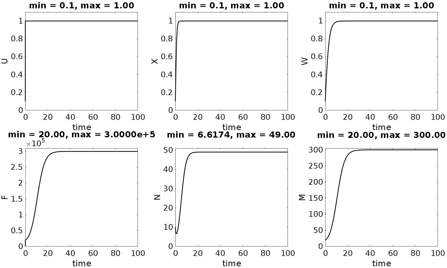
Figure 2: Case $E_{1}$. Plots of time evolution of the state variables.

Variable	t=0	t=100
U	$1.0000e-01$	$1.0000e+00$
F	$2.0000e+01$	$3.0000e+05$
X	$1.0000e-01$	$1.0000e+00$
N	$1.0000e+01$	$4.9000e+01$
W	$1.0000e-01$	$1.0000e+00$
M	$2.0000e+01$	$3.0000e+02$

Table 4: Case $E_{1}$. Initial (t=0) and final (t=100) configuration of the state variables.

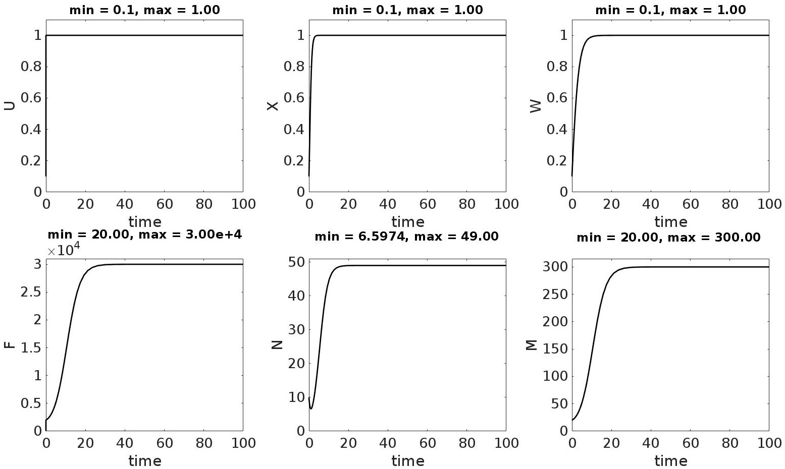
Figure 3: Case $E_{1}^{{}^{\prime}}$. Plots of time evolution of the state variables.

Variable	t=0	t=100
U	$1.0000e-01$	$1.0000e+00$
F	$2.0000e+01$	$3.0000e+04$
X	$1.0000e-01$	$1.0000e+00$
N	$1.0000e+01$	$4.9000e+01$
W	$1.0000e-01$	$1.0000e+00$
M	$2.0000e+01$	$3.0000e+02$

Table 5: Case $E_{1}^{{}^{\prime}}$. Initial (t=0) and final (t=100) configuration of the state variables.

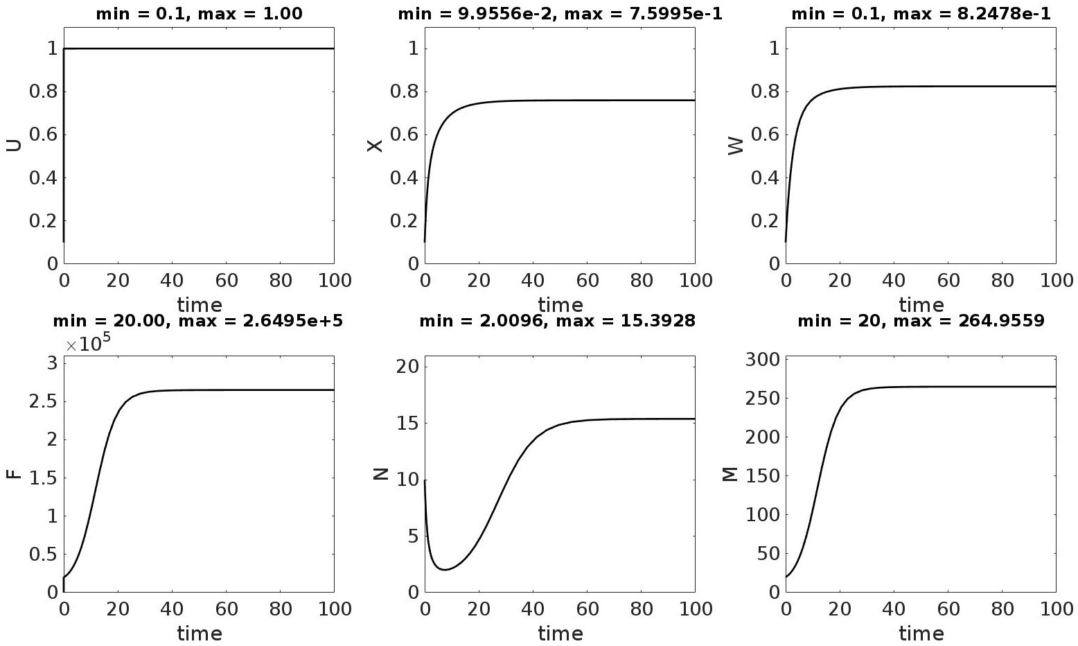
Figure 4: Case $E_{2}$. Plots of time evolution of the state variables.

Variable	t=0	t=100
U	$1.0000e-01$	$1.0000e+00$
F	$2.0000e+01$	$2.6495e+05$
X	$1.0000e-01$	$7.5995e-01$
N	$1.0000e+01$	$1.5393e+01$
W	$1.0000e-01$	$8.2478e-01$
M	$2.0000e+01$	$2.6496e+02$

Table 6: Case $E_{2}$. Initial (t=0) and final (t=100) configuration of the state variables.

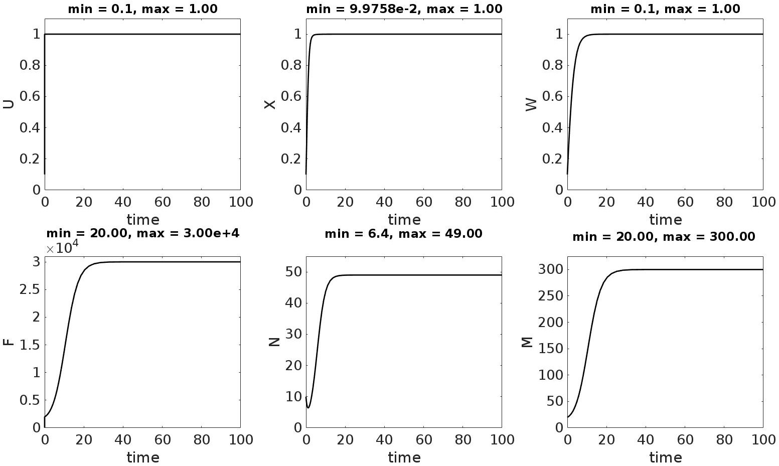
Figure 5: Case $E_{2}^{{}^{\prime}}$. Plots of time evolution of the state variables.

Variable	t=0	t=100
U	$1.0000e-01$	$1.0000e+00$
F	$2.0000e+01$	$3.0000e+04$
X	$1.0000e-01$	$1.0000e+00$
N	$1.0000e+01$	$4.9000e+01$
W	$1.0000e-01$	$1.0000e+00$
M	$2.0000e+01$	$3.0000e+02$

Table 7: Case $E_{2}^{{}^{\prime}}$. Initial (t=0) and final (t=100) configuration of the state variables.

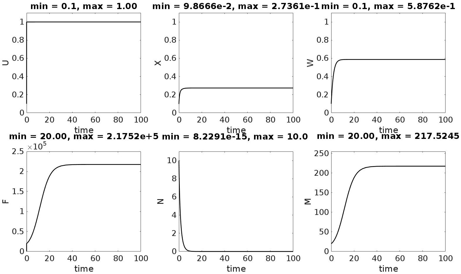
Figure 6: Case $E_{3}$. Plots of time evolution of the state variables.

Variable	t=0	t=100
U	$1.0000e-01$	$9.9999e-01$
F	$2.0000e+01$	$2.1752e+05$
X	$1.0000e-01$	$2.7360e-01$
N	$1.0000e+01$	$8.2291e-15$
W	$1.0000e-01$	$5.8762e-01$
M	$2.0000e+01$	$2.1752e+02$

Table 8: Case $E_{3}$. Initial (t=0) and final (t=100) configuration of the state variables.

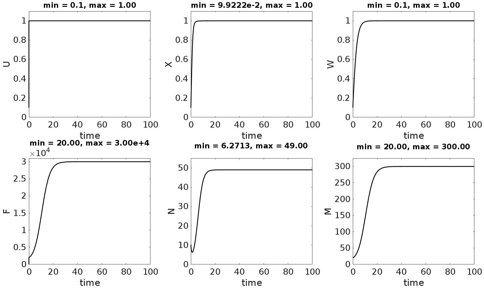
Figure 7: Case $E_{3}^{{}^{\prime}}$. Plots of time evolution of the state variables.

Variable	t=0	t=100
U	$1.0000e-01$	$1.0000e+00$
F	$2.0000e+01$	$3.0000e+04$
X	$1.0000e-01$	$1.0000e+00$
N	$1.0000e+01$	$4.9000e+01$
W	$1.0000e-01$	$1.0000e+00$
M	$2.0000e+01$	$3.0000e+02$

Table 9: Case $E_{3}^{{}^{\prime}}$. Initial (t=0) and final (t=100) configuration of the state variables.

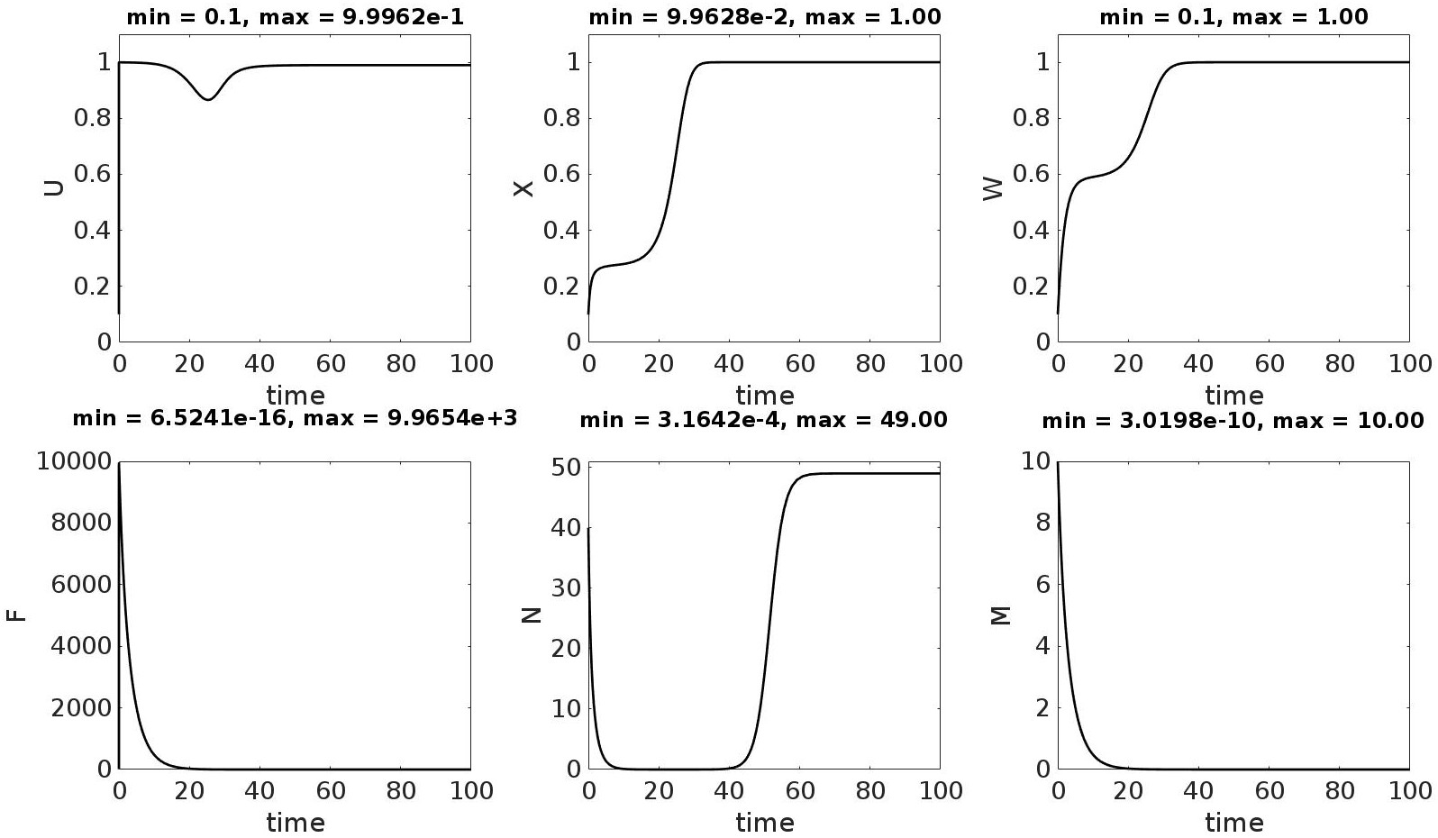
Figure 8: Case $E_{4}$. Plots of time evolution of the state variables.

Variable	t=0	t=100
U	$1.0000e-01$	$9.8974e-01$
F	$1.0000e+01$	$6.5241e-16$
X	$1.0000e-01$	$1.0000e+00$
N	$4.0000e+01$	$4.9000e+01$
W	$1.0000e-01$	$1.0000e+00$
M	$1.0000e+01$	$3.0198e-10$

Table 10: Case $E_{4}$. Initial (t=0) and final (t=100) configuration of the state variables.

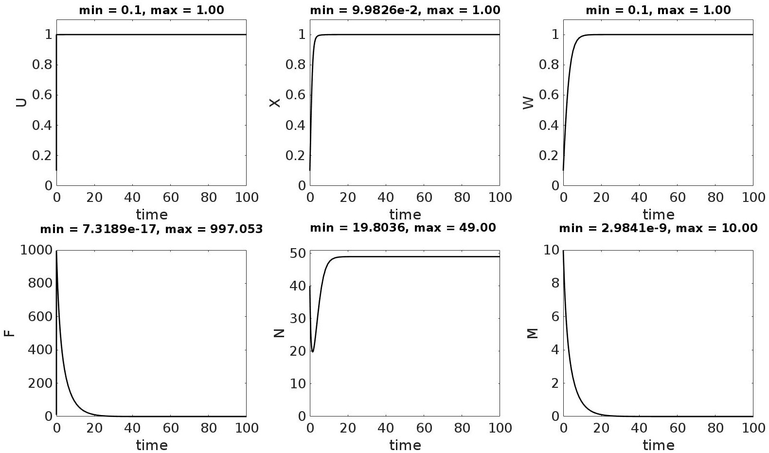
Figure 9: Case $E_{4}^{{}^{\prime}}$. Plots of time evolution of the state variables.

Variable	t=0	t=100
U	$1.0000e-01$	$1.0000e+00$
F	$1.0000e+01$	$7.3189e-17$
X	$1.0000e-01$	$1.0000e+00$
N	$4.0000e+01$	$4.9000e+01$
W	$1.0000e-01$	$1.0000e+00$
M	$1.0000e+01$	$2.9841e-09$

Table 11: Case $E_{4}^{{}^{\prime}}$. Initial (t=0) and final (t=100) configuration of the state variables.

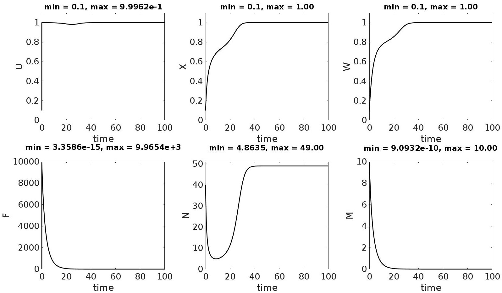
Figure 10: Case $\hat{E}_{4}$. Plots of time evolution of the state variables.

Variable	t=0	t=100
U	$1.0000e-01$	$9.9950e-01$
F	$1.0000e+01$	$3.3586e-15$
X	$1.0000e-01$	$1.0000e+00$
N	$4.0000e+01$	$4.9000e+01$
W	$1.0000e-01$	$1.0000e+00$
M	$1.0000e+01$	$9.0932e-10$

Table 12: Case $\hat{E}_{4}$. Initial (t=0) and final (t=100) configuration of the state variables.

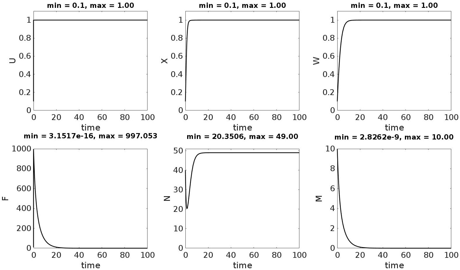
Figure 11: Case $\hat{E}_{4}^{{}^{\prime}}$. Plots of time evolution of the state variables.

Variable	t=0	t=100
U	$1.0000e-01$	$1.0000e+00$
F	$1.0000e+01$	$3.1517e-16$
X	$1.0000e-01$	$1.0000e+00$
N	$4.0000e+01$	$4.9000e+01$
W	$1.0000e-01$	$1.0000e+00$
M	$1.0000e+01$	$2.8262e-09$

Table 13: Case $\hat{E}_{4}^{{}^{\prime}}$. Initial (t=0) and final (t=100) configuration of the state variables.

7 Concluding remarks

The above analysis has shown that four main cases are feasible for the equilibria of the dynamical system describing the evolution of Xylella fastidiosa epidemics within olive orchard agroecosystems. The equilibrium $E_{1}$ corresponds to a disease free ecosystem (see Figure 2); equilibrium $E_{2}$ corresponds to coexistence of a non- trivial olive tree biomass and infective insects, which we may conjecture (also supported by the numerical experiments) is possible only for a sufficiently small value of $\lambda,$ i.e. for more resistant olive tree cultivars (see Figure 4); the equilibrium $E_{2}$ may degenerate into $E_{3}$ for a sufficiently large value of $\lambda,$ i.e. for less resistant olive tree cultivars, which leads to the complete disappearance of the olive tree biomass (see Figure 6). Finally the equilibria $E_{4}$ and $\widehat{E_{4}}$ correspond to eradication of the insect population, by a significant reduction of the weed reproduction rate (see Figures 8 and 10).

The outcomes of the numerical simulations, reported in Figures 3, 5, 7, 9, 11, elucidate the crucial role of the parameter $\chi.$ From Equation (13) we may recognize the role of $\displaystyle\frac{M}{\chi}$ as the effective carrying capacity of the insect population $F;$ for $\chi_{1}\leq\chi_{2}$ we have

$$\frac{M}{\chi_{1}}\geq\displaystyle\frac{M}{\chi_{2}},$$

which implies, for $\chi_{1},$ a possible larger population of insects, hence a possible larger infective insect population, which may lead to a larger force of infection on olive trees, thus making the coexistence of insects and trees unlikely.

Hence, once an epidemic has started, in absence of intervention our model predicts a possible full collapse of the olive tree biomass, with a significant socio-economic impact. About agronomic practices, the most interesting result concerns the role of weeds for the eradication of a X. fastidiosa epidemic. Indeed, according to our model, a sufficient reduction of the weed biomass may lead to a significant decay of the insect populations, and consequently to the eventual eradication of the epidemic. Weeds, also present in the relevant olive orchard, represent the main feeding resource of the insects at their juvenile stage. We have to be aware that insects juvenile feed on a large variety of both weeds and ornamental plants, so that a particular attention has to be paid not only to the usual spontaneous plants emerging in the olive orchard itself, but also to any kind of ornamental plant existing in its near neighborhood [19]. A second possible strategy for prevention and control of a X. fastidiosa epidemic, which has been confirmed by our analysis, concerns the substitution of the currently cultivated olive tree cultivars by more resistant ones. This approach has already been suggested by the local agriculture Authorities in Southern Apulia. But we have to take into account that, different from the usual good agronomic practice of weed elimination, the substitution of a cultivar is both money and time much more expensive; it takes a long time before a new planted or grafted tree reaches the level of production of an existing one. On the other hand, it goes without saying that the impact of the cultivar on the quality of the extracted olive oil can be dramatic for the local economy. As an example, Apulia has a great international reputation for the production of a variety of olive oil of outstanding quality, based on the current cultivar all over the region (see e.g. [9], https://bestoliveoils.org/brands/).

Once again, we wish to conclude by warning the readers that validation of the model proposed here represents a key issue: although we have tried to make explicit the assumptions underlying our model, they have not yet been validated by comparison with experimental data. Therefore we caution that our results are far from being conclusive for X. fastidiosa - P. spumarius olive tree epidemics. However, it is desirable that with further experiments, possibly driven by our models, additional features are added that make them more realistic, so that mathematical models might provide the foundations for designing optimal control strategies by the relevant public authorities.

References

- [1] Almeida, R.P.P., Blua, M.J., Lopes, J.R.S., Purcell, A.H., Vector transmission of Xylella fastidiosa: applying fundamental knowledge to generate disease management strategies. Ann. Entomol. Soc. Am., 98 (2005), 775-786.
- [2] Aniţa, S., Capasso, V., Scacchi, S., Controlling the spatial spread of a Xylella epidemic. Bull. Math. Biology, (2021) 83:32. doi: 10.1007/s11538-021-00861-z
- [3] Boscia, D., Altamura, G., Saponari, M., Tavano, D., Zicca, S., Pollastro, P., Silletti, M.R., Savino, V.N., Martelli, G.P., Delle Donne,A. , Mazzotta, S., Signore, P.P., Troisi, M., Drazza, P., Conte, P., D’ Ostuni, V., Merico, S., Perrone, G., Specchia, F., Stanca, A., Tanieli, M., Incidenza di Xylella in oliveti con disseccamento rapido. Informatore Agrario, 27(59-64) (2017), 47-50.
- [4] Brunetti, M., Capasso, V., Montagna, M., Venturino, E., A mathematical model for Xylella fastidiosa epidemics in the Mediterranean regions. Promoting good agronomic practices for their effective control. Ecol Model 432 (2020)109204. doi: 10.1016/j.ecolmodel.2020.109204
- [5] Capasso V. Mathematical Structures of Epidemic Systems, 2nd revised printing, Lecture Notes Biomath., Vol. 97. Heidelberg: Springer-Verlag; 2009.
- [6] Carlucci, A., Lops, F., Marchi, G., Mugnai, L., Surico, G., Has Xylella fastidiosa “chosen” olive trees to establish in the Mediterranean basin? Phytopathologia Mediterranea, 52 (2013), 541-544.
- [7] Cornara, D., et al., Transmission of Xylella fastidiosa by naturally infected Philaenus spumarius (Hemiptera, Aphrophoridae) to different host plants. J. Appl. Entomol. 141 (2017), 80-87.
- [8] Dietz, K., Overall population patterns in the transmission cycle of infectious disease agents. In Population Biology of Infectious Diseases, R.M. Anderson, R.M. May, Editors. Life Sciences Research Reports, Vol. 25. Heidelberg: Springer-Verlag; 1982.
- [9] Dugo, L., Russo, M., Cacciola, F. et al., Determination of the Phenol and Tocopherol Content in Italian High-Quality Extra-Virgin Olive Oils by Using LC-MS and Multivariate Data Analysis. Food Anal. Methods 13 (2020), 1027–1041. doi: 10.1007/s12161-020-01721-7
- [10] Fierro, A., Liccardo, A., Porcelli, F. (2019). A lattice model to manage the vector and the infection of the Xylella fastidiosa on olive trees. Scientific Reports, 9(1), 8723.
- [11] Jeger, M. et al. (EFSA PLH Panel, Updated pest categorisation of Xylella fastidiosa. EFSA Journal, 16(7)(2018), e05357. doi: 537 10.2903/j.efsa.2018.5357.
- [12] Martelli, G. P., Boscia, D., Porcelli, F., Saponari, M. , The olive quick decline syndrome in south-east Italy: a threatening phytosanitary emergency. European Journal of Plant Pathology, 144(2) (2016), 235-243.
- [13] Redak, R.A., Purcell, A.H., Lopes, J.R.S., Blua, M.J., Mizell, R.F. III, Andersen, P.C., The biology of xylem fluid-feeding insect vectors of Xylella fastidiosa and their relation to disease epidemiology, applying fundamental knowledge to generate disease management. Annu. Rev. Entomol. 49 (2004), 243-270.
- [14] Saponari, M., Boscia, D., Altamura, G., Loconsole, G., Zicca, S., D’Attoma, G., Morelli, M., Palmisano, F., Saponari, A., Tavano, D., Savino, V. N., Dongiovanni, C., Martelli, G. P., Isolation and pathogenicity of Xylella fastidiosa associated to the olive quick decline syndrome in southern Italy. Scientific reports, 7 (2017), 17723. DOI:10.1038/s41598-017-17957-z.
- [15] Saponari, M., Giampetruzzi, A., Loconsole, G., Boscia, D., Saldarelli, P., Xylella fastidiosa in olive in Apulia: Where we stand. Phytopathology, 109(2) (2018), 175-186.
- [16] Schneider, K., van der Werf, W., Cendoya, M., Maurits, M., Navas-Cortes, J.A., Impact of Xylella fastidiosa subspecies pauca in European olives. PNAS, 117 (2020), 9250-9259.
- [17] Silva S. E., et al., Differential survival and reproduction in colour forms of Philaenus spumarius give new insights to the study of its balanced polymorphism. Ecological Entomology, 40 (2015), 759-766.
- [18] Villalobos, F. J., Testi, L., Hidalgo, J., Pastor, M., Orgaz, F. (2006). Modelling potential growth and yield of olive (Olea europaea L.) canopies. European Journal of Agronomy, 24(4), 296-303
- [19] White, S. M., Bullock, J. M., Hooftman, D. A., Chapman, D. S., Modelling the spread and control of Xylella fastidiosa in the early stages of invasion in Apulia, Italy. Biological Invasions, 19(6)(2017), 1825-1837.
- [20] Yurtsever, S., On the polymorphic meadow spittlebug, Philaenus spumarius (L.) (Homoptera: Cercopidae). Turkish Journal of Zoology, 24(4) (2000), 447-460.