Computer-aided Interpretable Features for Leaf Image Classification

Abstract

Plant species identification is time-consuming, costly, and requires lots of effort, and expert knowledge. The studies on medicinal plant identification are often performed based on medicinal plant leaf images. The is because plant leaves contain a large number of diverse sets of features such as shape, veins, edge features, apices, etc. that are useful in identifying different medicinal plants. In recent, many researchers use deep learning methods to classify plants directly using plant images. While deep learning models have achieved great success, the lack of interpretability limits their widespread application. To overcome this, we explore the use of interpretable, measurable, and computer-aided features extracted from plant leaf images. Image processing is one of the most challenging, and crucial steps in feature extraction. The purpose of image processing is to improve the leaf image by removing undesired distortion. The main image processing steps of our algorithm involve: i) Convert original image to RGB (Red-Green-Blue) image, ii) Gray scaling, iii) Gaussian smoothing, iv) Binary thresholding, v) Remove the stalk, vi) Closing holes, and vii) Resize the image. The next step after image processing is to extract features from plant leaf images. We introduced 52 computationally efficient features to classify plant species. These features are mainly classified into four groups as i) shape-based features, ii) color-based features, iii) texture-based features, and iv) scagnostic features. Length, width, area, texture correlation, monotonicity, and scagnostics are to name a few of them. We explore the ability of features to discriminate the classes of interest under supervised learning and unsupervised learning settings. For that, supervised dimensionality reduction technique, Linear Discriminant Analysis (LDA), and unsupervised dimensionality reduction technique, Principal Component Analysis (PCA) are used to convert and visualize the images from digital-image space to feature space. All the applications are performed on Flavia and Swedish open-source benchmark leaf datasets. The results show that the features are sufficient to discriminate the classes of interest under both supervised and unsupervised learning settings. The results of this study are beneficial for the researchers working in the field of developing automated plant identification and classification systems.

Keywords Medicinal  $\cdot$ Image processing  $\cdot$ Feature extraction  $\cdot$ LDA  $\cdot$ PCA

1 Introduction

Leaf identification is becoming very popular in classifying plant species. Plant leaf contains a significant number of features that can help people to identify and classify plant species. From a medical perspective, medicinal plants are usually identified by practitioners based on years of experience through sensory or olfactory senses. The other method of recognizing these plants involves laboratory-based testing, which requires trained skills, data interpretation which is costly and time-intensive. Automatic ways to identify medicinal plants are useful especially for those that are lacking experience in medicinal plant recognition. Statistical machine learning techniques play a crucial role in the development of automatic systems to identify medicinal plants. In developing such a system input features play an important role. The main aim of this paper is to introduce interpretable features that can be computed based on plant leaf images. Image processing and feature extraction play crucial roles in developing a workflow to achieve the aim of this research.

The main aim of image processing is to extract important features by removing undesired noise and distortion (Wäldchen and Mäder, 2018). Image processing steps include image segmentation (Anantrasirichai et al., 2017), image orientation, cropping, grey scaling, binary thresholding, noise removal, contrast stretching, threshold inversion, image normalization, and edge recognition are some of the image processing techniques applied in recent research. These steps can be applied parallel or individually, several times until the quality of the leaf image reaches a specific threshold.

The second step is feature extraction, which identifies and encodes relevant features from leaf images (Wäldchen and Mäder, 2018). This is a challenging task due to the structural diversity of the leaf images. Therefore, in recent years, many researchers use deep learning methods to classify plants directly using plant images (Wu et al., 2007a; Azlah et al., 2019; Herdiyeni and Wahyuni, 2012). While deep learning models have achieved great success, most models remain complex black boxes. The lack of interpretability limits their widespread application.

A digital image is a combination of pixels from three different color planes red, green, and blue. Images are stored in computers as three separate matrices corresponding to the red, green, and blue color channels of the image. The three separate matrices corresponding to intensities of colors at different positions of the image (Gonzalez and Woods, 2006).

The main aim of feature extraction is to reduce the dimensionality of this information by obtaining measurable patterns of leaf images. For example, shape, color, and texture are some of the patterns that may be observed. In this paper, we introduce a collection of interpretable, measurable, and computer-aided features that are useful in image leaf classification. This feature collection includes several pre-established features identified through a thorough review of the literature. Other than existing features, we introduce several features computed based on the Cartesian coordinate of the images. Furthermore, we explore the ability of features to discriminate the class of interest under a supervised learning setting and an unsupervised learning setting.

The paper is organized as follows. Section 2, describes the steps of image processing. Preprocessing is necessary before extracting features from the images. Section 3, discusses feature extraction in in-detail because features are highly influenced by the plant species to be classified. Under this section, we discuss mainly four types of features as shape, color, texture, and scagnostics and how to extract them. Section 4, presents empirical application. This section consists of details about the datasets that are used to explain the applications, and visualization of leaf images in the feature space using supervised, and unsupervised dimensionality reduction techniques. Section 5, consists of a summary of the software and packages used to extract the features. Some discussion about the outputs and concluding remarks are given in the last section.

2 Image Processing

Image processing is an essential step to reduce noise and content enhancement while keeping its features intact (Goyal et al., 2018). The workflow we use to process images in this paper is shown in Figure 1. This includes seven main steps. They are: i) converting BGR (Blue-Green-Red) image to RGB (Red-Green-Blue), ii) gray scaling, iii) Gaussian filtering, iv) binary thresholding, v) remove stalk, vi) close holes, and vii) image resizing. Some of these steps are applicable only to specific images. For example, apply to remove stalk is applicable only to leaf images that have a stalk.

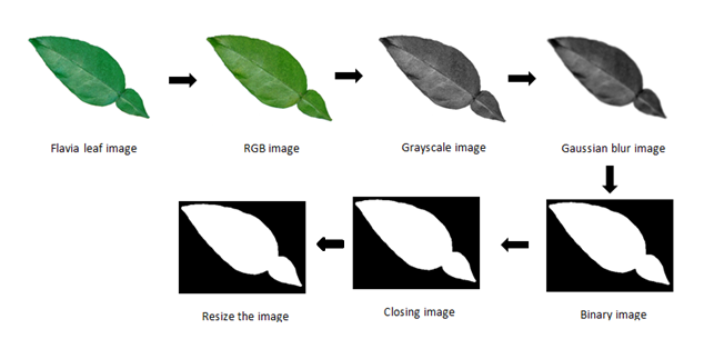
Figure 1: Image processing workflow.

In this study, we focus on leaves with a simple arrangement as shown in Figure 2(c). A single leaf that is never divided into smaller leaflet units is known as a leaf with a simple arrangement. This type of leaf is attached to a twig by its stem or the petiole. The margins, or edges, of the leaf, can be smooth, lobed, or toothed (see Figure 2(b)).

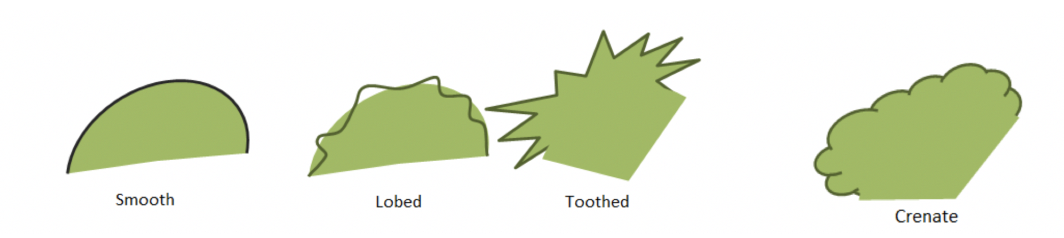
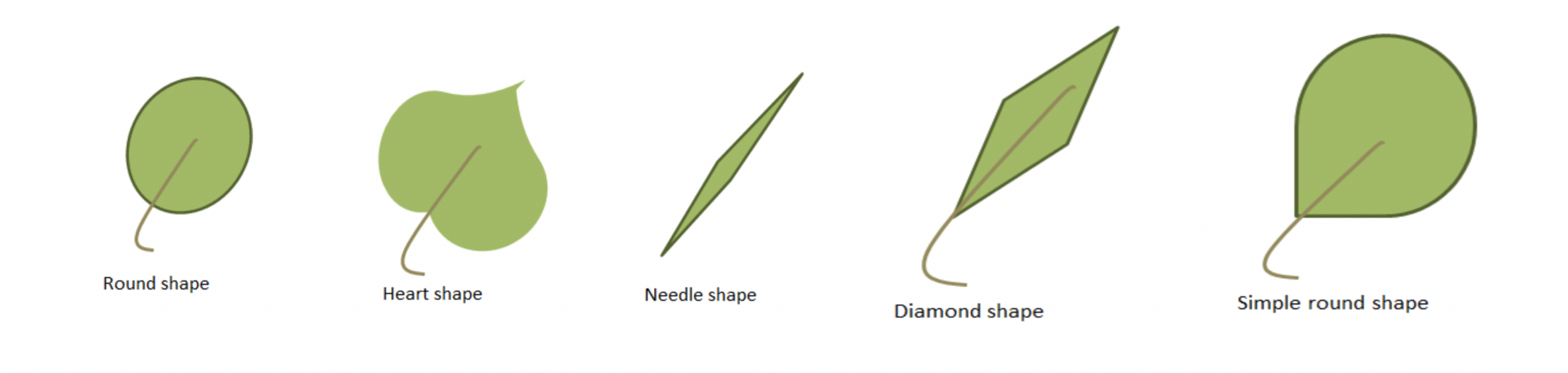
(a) Edge types of leaves focus in the study.

(b) Shape illustrations

(c) A leaf with a simple arrangement.

Figure 2: Leaf feature structures considered in the analysis

2.1 Step 1: Converting BGR (Blue-Green-Red) Image to RGB (Red-Green-Blue)

BGR and RGB are conventions for the order of the different colour channels. They are not colour spaces. When converting BGR image to RGB, there are no computations other than switching around the order. Different image processing libraries have different pixel ordering. To be compatible with other libraries, we convert the BGR image into RGB format. For example, when we read an image using the OpenCV library in Python by default it interprets BGR format, but when we plot the image it takes the RGB format in matplotlib package in Python.

2.2 Step 2: Grayscaling

Gray-scaling is the process of converting an image to shades of gray from other colour spaces like RGB. This helps to increase the contrast and intensity of images (Goyal et al., 2018). Gray scale images require only one single byte for each pixel whereas colour (RGB) image requires 3 bytes for each pixel. Hence, gray-scaling reduces the dimension of an image.

Another advantage of using gray-scaled images is to reduce model complexity. Consider an example of a training neural article on RGB images of $20\times 20\times 3$ pixel. The input layer will have 1200 input nodes. Whereas for gray scaled images the same neural network will need only 400 ($20\times 20$) input node.

2.3 Step 3: Gaussian Filtering (Gaussian Blurring/Gaussian Smoothing)

Gaussian smoothing is an image smoothing technique. Image smoothing techniques are used to remove the noise that can be occurred due to the source (camera sensor). Image smoothing techniques help in smoothing images and removing intensity edges.

A Gaussian function is used to blur the image. It is a linear filter. We used the OpenCV package in Python for Gaussian smoothing. The width and height of the Gaussian kernel must be positive and odd. Furthermore, the kernel standard deviation along the x and y-axis should be specified. When the kernel standard deviation along the x-axis is specified, kernel standard deviation along the y-axis is taken as equal to the kernel standard deviation along the x-axis. However, if both kernel standard deviations are given as zeros, the calculations are done using the kernel size. In our research, the width and height of the kernel are defined as 55 and the kernel standard deviation along the x-axis is assigned as zero. An example of applying Gaussian smoothing to an image is shown in Figure 3.

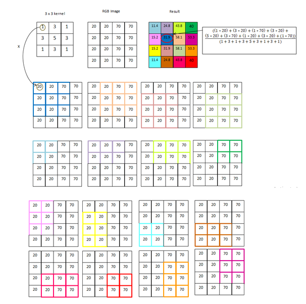
Figure 3: Example of applying Gaussian smoothing

2.4 Step 4: Binary Thresholding

Thresholding is a segmentation technique that is used to separate the foreground from its background. Thresholding converts the gray-scale images into binary images according to the threshold value. If the pixel value is smaller than the threshold value, the pixel value is set as 0, and if not the pixel value is set to a maximum value which is generally 255. The thresholding technique is done on the gray-scale images in computer vision.

We used Otsu’s binarization adaptive thresholding after Gaussian filtering to convert color images to binary images. The reason for using Otsu’s binarization method is, it automatically determines the optimal threshold value.

Otsu’s Thresholding

Nobuyuki Otsu introduced Otsu’s method which is defined for a histogram of grayscale values of a histogram ($ghist_{I}$) of an input image $Im$. To segment an image $Im$ into two subsets of pixels Otsu’s method calculates an optimal threshold $\tau$. The number of pixel locations of the grayscale image is defined as $|\Omega|$. The algorithm maximizes the variance $\sigma^{2}$ between the two subsets (Within-class-variance) to find the threshold $\tau$. The variance $\sigma^{2}$ is defined as

$$\sigma^{2}=P_{1}(\mu_{1}-\mu)^{2}+P_{2}(\mu_{2}-\mu)^{2}=P_{1}P_{2}(\mu_{1}-\mu_{2})^{2},$$

where $\mu$ is the mean of the histogram, $\mu_{1}$ and $\mu_{2}$ are the mean values of first and second subset respectively. The corresponding class probabilities, $P_{1}$ and $P_{2}$ are defined as follows,

$$P_{1}=\frac{\sum_{i=0}^{u}ghist_{I}(i)}{|\Omega|}\text{, and }P_{2}=\frac{\sum_{i=u+1}^{255}ghist_{I}(i)}{|\Omega|},$$

where $u$ is the candidate threshold and the maximum gray level ($G_{max}$) is assumed as 255. To find the optimal threshold $\tau$ for segmenting image $Im$, all candidate thresholds are evaluated this way. The algorithm of Otsu’s method is defined as follows:

Create a histogram for the grayscale image

Set the histogram variance $S_{max}=0$

while $u<G_{max}$ do

Compute $\sigma^{2}=P_{1}*P_{2}(\mu_{1}-\mu_{2})^{2}$

if $\sigma^{2}>S_{max}$ then

$S_{max}=\sigma^{2}$

$\tau=u$

end if

Set $u=u+1$

end while

Table 1: Otsu’s method

For example, assume that candidate threshold value $u$ is 2. Therefore, the image is separated into two classes, which are class 1 ($\text{pixel value}<=2$ ) and class 2 ($\text{pixel value}>2$). Class 1 represents the background and class 2 represents the foreground of the grayscale image. According to Figure 4, there are 9 pixel locations. The associated measurements are

$$P_{1}=\frac{5}{9},P_{2}=\frac{4}{9},\mu_{1}=\frac{(0*2)+(1*1)+(2*2)}{(2+1+2)}=1,\mu_{2}=\frac{(3*3)+(4*1)}{(3+1)}=\frac{13}{4},$$

$$\sigma^{2}=\frac{5}{9}*\frac{4}{9}*(1-\frac{13}{4})^{2}=1.25.$$

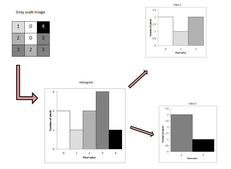
Figure 4: Example of Otsu’s binary thresholding

2.5 Step 5: Image Resizing

In this study we use two different benchmark leaf image datasets: i) Flavia: 1907 fully color images of 32 classes of leaves (Wu et al., 2007b) and ii) Swedish: 1125 images from 15 different plant species (Söderkvist, 2001). Flavia and Swedish images have two different image sizes. To compare the results on different datasets, to improve the memory storage capacity, and to reduce computational complexity the leaf images are resized to a fixed resolution. In our study, the leaf images have been resized to [1600 x 1200px] which is the size of Flavia leaf images.

Other than the main image processing techniques discussed above, the following techniques are applied to some images where necessary after image thresholding.

‘

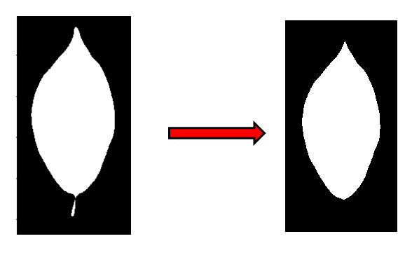
(a) Remove stalk

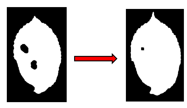
(b) Closing holes

Figure 5: Other image processing steps: (a) Remove the stalk, and (b) close holes

2.5.1 Remove the Stalk

As shown in Figure 5(a), this is used to remove the stalk of the image. Remove the petiole (stalk) of the leaf image is another version of the thresholding process. Thresholding is applied after finding the sure foreground area. To find the sure foreground area, the distance transform technique is used. The binary image is used as the input of the distance transform technique. In the distance transform technique, an image is created by assigning a number for each object pixel that corresponds to the distance to the nearest background pixel. The distance is calculated using the Euclidean distance. After finding the sure foreground area, Otsu’s binarization is applied again as the thresholding technique.

2.5.2 Closing Holes

Holes inside leaf areas occur due to plant disease, light reflection, and noise. As shown in Figure 5(b) closing holes is used to remove small holes inside the foreground objects. This is achieved by pulling background pixels to foreground pixels. The closing holes are also known as dilation and while erosion does the opposite, which is open holes. This step is performed on a binary image.

Erosion

The basic idea of Erosion is that erodes the boundaries of the foreground object. Since the input is a binary image, a pixel in the original image is either 1 or 0. If all the pixels under the kernel is 1, a pixel of the original image is considered as 1, otherwise made to zero (eroded). This means that depending upon the size of the kernel all pixels near the boundary will be discarded. Therefore the thickness or size of the foreground object decreases (the white region of the image decreases).

Dilation

The opposite of erosion is defined as dilation. If at least one pixel under the kernel is 1, the pixel element is 1 in Dilation. It tends to increase the foreground of the image or the white region of the object.

3 Leaf Image Features

In the identification of plant species using leaf images, features of leaves play an important role, because each leaf possesses a unique feature that it makes different from others. The previous studies (Azlah et al., 2019; Mingqiang et al., 2008; Sun et al., 2017) use deep learning neural networks to classify medicinal plants based on pixel-based images. Given the leaf images, deep learning models automatically identify features based on the pixel space of the images. While deep learning models have achieved great success, the lack of interpretability of features limits their widespread application. To overcome this, we explore the use of interpretable, measurable, and computer-aided features extracted from plant leaf images. We identified 52 features. The features are classified into four groups as i) shape-based features, ii) color-based features, iii) texture-based features and iv) scagnostic features. In this study, we considered 21 shape features, 4 texture features, 6 color-based features, and 21 scagnostic features.

3.1 Shape Features

When identifying real-world objects, the shape is known as an essential sign for humans. We use the shape descriptors introduced by (Wäldchen and Mäder, 2018). In addition to that, we introduce several new shape features such as the number of convex points, x and y coordinates of the center, number of maximum and minimum points, correlation of Cartesian contour points, etc. The shape features should be invariant to a certain class of geometric transformation of the object. The main geometric transformations are rotation reflection, scaling, and translation (see Figure 6). The shape features we considered in this study are invariant to the rotation and reflection. All the shape features are extracted from the binary images.

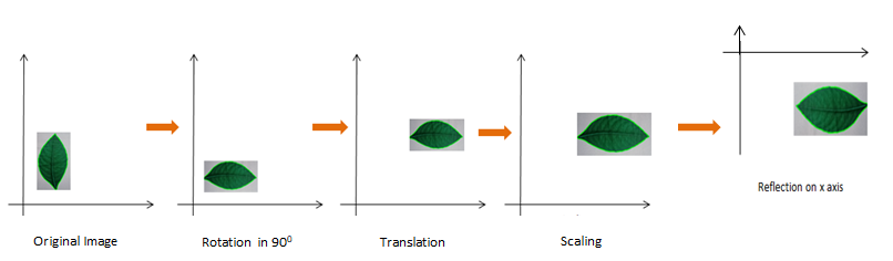
Figure 6: Illustration of geometric transformation

Extraction of image contour plays an important role in measuring the shape of an image. Simply contour (see Figure 7) is a curve joining all the continuous points (along the boundary), having the same color or intensity.

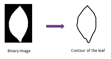
Figure 7: Extract contour of the leaf image

To extract the contour of the leaf, the leaf should be placed properly in the center of a white paper. If the image is placed as shown in Figure 8, as a result of inappropriate translation (a) and inappropriate scaling (b), problems arise in the calculations of the contour. Furthermore, it is difficult to recognize the contour, when the image is too small.

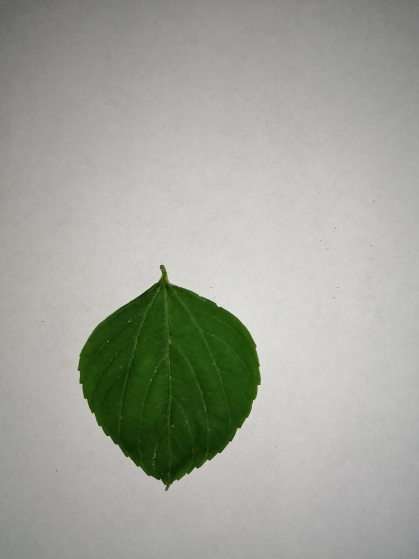
(a)

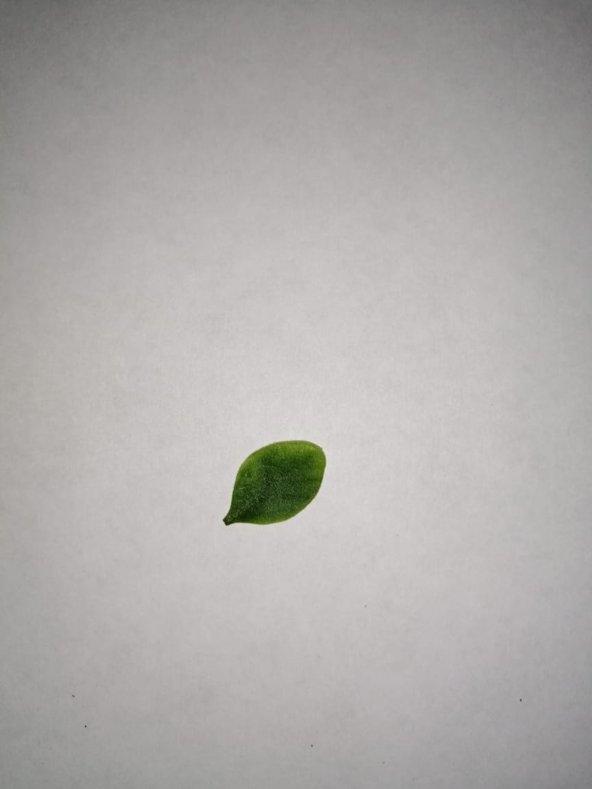
(b)

Figure 8: (a) Inappropriate translation, (b) Inappropriate scaling

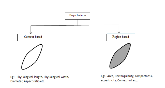
Figure 9: Categorization of shape features

Shape features can be classified into two main categories as contour-based and region-based features (Wäldchen and Mäder, 2018). As illustrated in (Wäldchen and Mäder, 2018), contour-based shape features are computed based on the contour of a shape, whereas region-based shape features are extracted from the whole region of a shape (see Figure 9).

In this study, we use 6 initial shape features that are used to derive 12 shape features. The 6 initial features are i) diameter, ii) physiological length, iii) physiological width, iv) area, v) perimeter, and vi) eccentricity.

3.1.1 Diameter ($F_{1}$)

Diameter is defined as the longest distance between any two points on the margin of the leaf (Wäldchen and Mäder, 2018). To calculate the diameter of the leaf image, first, we need to find the contour of the leaf image. Then we need to select all pairs of contour points and measure the Euclidean distance between the two points separately. Finally, we have to find the maximum distance among the calculated distances.

3.1.2 Physiological length ($F_{2}$) and Physiological width ($F_{3}$)

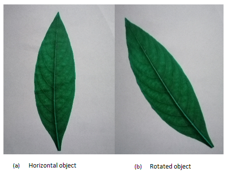
Figure 10: (a) Straight (horizontal or vertical) and (b) Rotated leaf image

According to the authors in Azlah et al. (2019), the physiological length is “measured based on the main vein of the leaf, as it stretches from the main vein to the end tip.” We use the definition by Azlah et al. (2019), the physiological width is “the span of leaf viewed from one side to the other, from the leftmost point to the rightmost point of leaf”. There are straight (horizontal or vertical) and angled leaf images in our datasets, Flavia and Swedish (see example Figure 10). There are two types of bounding rectangles.

1. Straight bounding rectangle: This is a straight rectangle that does not consider the rotation of the object (see Figure 10 (a)).

1. Rotated rectangle: This bounding rectangle is drawn with minimum background area. Therefore the rotation of the object is also considered (see Figure 10 (b)).

The straight bounding rectangle is enough to extract the physiological length and physiological width of straight (horizontal or vertical) leaf images. However, the straight bounding rectangle is not suitable to compute the physiological length and physiological width of angled leaf images. To solve this problem, we considered a rotated rectangle rather than a bounded rectangle in computing shape features of angled images. As shown in Figure 11, the length of the rotated rectangle is considered as the physiological length ($F_{2}$) and the width of the rotated rectangle is considered as the physiological width ($F_{3}$).

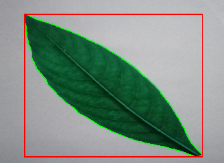
(a)

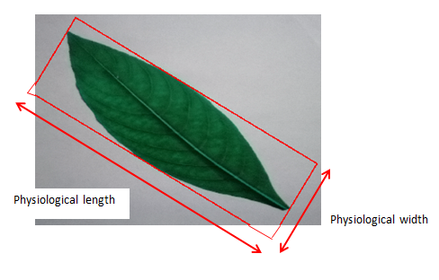
(b)

Figure 11: (a) Straight bounded rectangle of a rotated leaf image, (b) Rotated rectangle of angled leaf image (b)

3.1.3 Area ($F_{4}$)

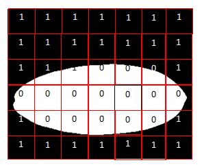
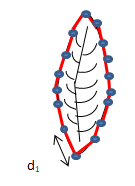
(a) Measure the area

(b) Perimeter

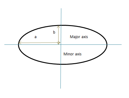
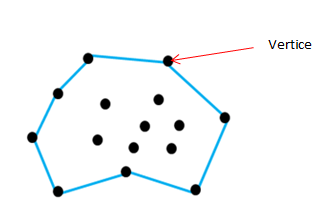
(c) Ellipse

(d) Convex hull

Figure 12: Illustration of (a) area, (b) perimeter, (c) ellipse, and (d) convex hull

The area is computed after applying the thresholding process. Next, we need to extract the best contour, and based on that contour area is measured. The number of 0 pixels covered by the contour is the measure of the area of the leaf image (Azlah et al., 2019).

3.1.4 Perimeter ($F_{5}$)

As shown in Figure 12(b) perimeter is defined as the summation of Euclidean distance of all continuous neighboring points in the contour. Let $n$ be the number of distances around the contour, then the perimeter is defined as

$$F_{5}=\sum_{i=0}^{n}d_{i}.$$ (1)

3.1.5 Eccentricity ($F_{6}$)

Eccentricity is a characteristic of any conic section of a leaf (Azlah et al., 2019). Eccentricity is defined that how much the ellipse actually varying being circular. Eccentricity is calculated using the equation 2 as

$$F_{6}=\sqrt{1-\frac{b^{2}}{a^{2}}},$$ (2)

where $a$ is semi-major axis and $b$ is semi-minor axis (see Figure 12(d)).

The eccentricity of an ellipse is varied between 0 and 1. If eccentricity is 0, then we obtain a circle whereas eccentricity is 1, then we obtain an ellipse (see Figure 13(c)).

3.1.6 Number of Convex Points ($F_{21}$) and Verticies

Wilkinson et al. (2005) defined a convex hull as a “hull that contains all the straight line segments connecting any pair of points in its interior.” The convex hull bounds a single polygon (see Figure 12(d)). We introduced two new features computed based on the convex hull: i) Number of convex points ($F_{21}$) and ii) Number of convex vertices ($F_{7}$).

3.1.7 Roundness/ Circularity

Roundness is named as aka form factor, circularity, or isoperimetrical factor. Roundness illustrates the difference between the leaf and a circle. Equation 3 is used to calculate roundness. Figure 13(c) visual explanation for roundness measure. The roundness is measured by

$$R=\frac{4\pi F_{4}}{{F_{5}}^{2}}.$$ (3)

3.1.8 Compactness

Compactness is closely related to roundness. Compactness measures that how compatible the leaf fits a circle area (see Figure 13(e)). The compactness is measured using

$$C=\frac{{F_{5}}^{2}}{F_{4}}.$$ (4)

3.1.9 Convexity

Convexity measures the curvature of the convex hull.

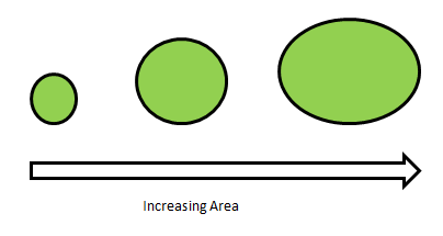
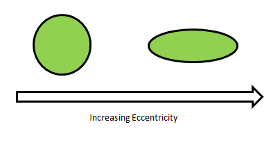
(a) Area

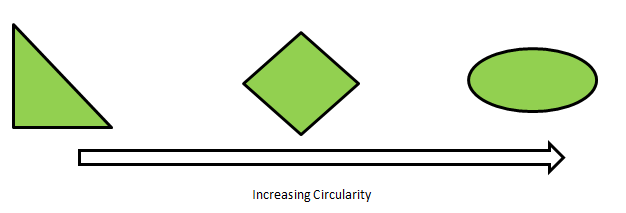
(b) Eccentricity

(c) Circularity

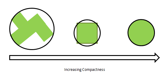
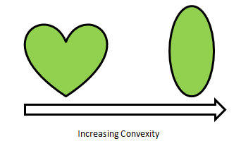
(d) Compactness

(e) Convexity

Figure 13: Variations in shapes as the values of features increase.

The equations and software packages used to compute shape features are shown in Table LABEL:tab:table1.

Table 2: Summary of shape features.

Shape feature	Feature name	Figure	Formula	Range	Software package
$F_{1}$	Diameter		see definition $F_{1}$	[0,$\infty$]	combinations, numpy
$F_{2}$	Physiological length		see definition $F_{2}$	[0,$\infty$)	OpenCV
$F_{3}$	Physiological width		see definition $F_{3}$	[0,$\infty$)	OpenCV
$F_{4}$	Area		see definition $F_{4}$		OpenCV
$F_{5}$	Perimeter		see definition $F_{5}$	[0,$\infty$)	OpenCV
$F_{6}$	Eccentricity		see definition $F_{6}$	[0,1]	OpenCV
$F_{7}$, $F_{8}$	x and y coordinate of center				scipy.ndimage
$F_{9}$	Aspect ratio		$F_{9}=\frac{F_{2}}{F_{3}}$	[0,$\infty$)	-
$F_{10}$	Roundness/ Circularity		eq:3	[0,$\infty$)	numpy
$F_{11}$	Compactness		eg:4	(0,$\infty$)	-
$F_{12}$	Rectangularity		$F_{12}=\frac{{F_{5}}^{2}}{F_{4}}$	(0,$\infty$)	-
$F_{13}$	Narrow factor		$F_{13}=\frac{F_{1}}{F_{2}}$	[0,$\infty$)	-
$F_{14}$	Perimeter ratio of diameter		$F_{14}=\frac{F_{5}}{F_{1}}$	[0,$\infty$)	-
$F_{15}$	Perimeter ratio of physiological length		$F_{15}=\frac{F_{5}}{F_{2}}$	[0,$\infty$)	-
$F_{16}$	Perimeter ratio of physiological length and width		$F_{16}=\frac{F_{5}}{F_{2}*F_{3}}$	[0,$\infty$)	-
$F_{17}$	Perimeter convexity		$F_{17}=\frac{\text{Perimeter of convex hull}}{F_{5}}$	[0,$\infty$)	OpenCV
$F_{18}$	Area convexity		$F_{18}=\frac{(\text{Area of convex hull}-F_{4})}{F_{4}}$	[0,$\infty$)	OpenCV
$F_{19}$	Area ratio of convexity		$F_{19}=\frac{F_{4}}{\text{Area of convex hull}}$	[0,$\infty$)	OpenCV
$F_{20}$	Equivalent diameter		$F_{20}=\sqrt{\frac{4*F_{4}}{\pi}}$	[0,$\infty$)	numpy
$F_{21}$	Number of convex points		number of convex points	[0,$\infty$)	OpenCV

3.2 Texture Features

Texture features are used to describe the surface or the appearance of the leaf image. Texture can be assessed using a group of pixels. Color is a property of a pixel. The texture is defined as a feeling of various materials to human touch and texture is quantified based on visual interpretation of this feeling. The leaf surface is a natural texture that has random persistent patterns and does not show detectable quasi-periodic structure (Wäldchen and Mäder, 2018). Therefore to describe the natural texture patterns of the leaf fractal theory (Wäldchen and Mäder, 2018) is the best approach.
      The In this study we used Haralick texture features (Dean, 1999). Haralick texture features are functions of the normalized GLCM (Gray Level Co-occurrence Matrix) is a common method to represent image texture.

$$GLCM=\begin{bmatrix}h(1,1)&h(1,2)&\cdot&\cdot&\cdot&h(1,n)\\ h(2,1)&h(2,2)&\cdot&\cdot&\cdot&h(2,n)\\ \cdot&\cdot&\cdot&&&\cdot\\ \cdot&\cdot&&\cdot&&\cdot\\ \cdot&\cdot&&&\cdot&\cdot\\ h(n,1)&h(n,2)&\cdot&\cdot&\cdot&h(n,n)\end{bmatrix}$$

The GLCM is square with dimension $n$, where $n$ is the number of gray levels in the image. Let $h(a,b)$ is the probability that a pixel with value $a$ will be found adjacent to a pixel of value $b$. Then $h(a,b)$ is defined as

$$h(a,b)=\frac{\text{Number of times a pixel with value a is adjacent to a pixel with value b}}{\text{Total number of such comparisons made}}.$$

In order to calculate $h(a,b)$, adjacency can be defined to occur in each of four directions in a 2D (see Figure 16), square pixel image (horizontal, vertical, left and right diagonals - see equation 14).

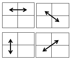
Figure 14: Four directions of adjacency as defined for calculation of the Haralick texture features

The Haralick statistics are calculated based on the matrices generated using each of these directions (see Figure 15) of adjacency . Haralick introduced 14 statistics to describe the texture of the image based on the four co-occurrences matrices generated (Dean, 1999). In this research, we only used the following 4 statistics among 14 of them, because most of the researchers used these 4 statistics as texture features (see Figure 3) of leaf images. All the texture features are extracted from the grayscale image. Texture features are calculated from the mahotas package in Python. Table 3 shows the definitions of texture features.

Texture feature	Feature name	Detailed description	Formula	Value range
$F_{22}$	Contrast	Measures the relation or difference between the highest and lowest gray levels of the GLCM	$\frac{\sum_{a=1}^{columns}\sum_{b=1}^{rows}(a-b)^{2}h(a,b)}{\text{Number of gray levels}-1}$	[0,$\infty$]
$F_{23}$	Entropy	Measures the randomness which means that how uniform the image is	$-\sum_{a=1}^{columns}\sum_{b=1}^{rows}h(a,b)log_{2}(h(a,b))$	[$-\infty$,0]
$F_{24}$	Correlation	Measurement of dependence of gray levels of the GLCM. It measures that how a particular pixel is correlated to it’s neighbor pixel over the whole image	$\frac{\sum_{a=1}^{columns}\sum_{b=1}^{rows}(ab)h(a,b)-\mu_{x}\mu_{y}}{\sigma_{x}\sigma_{y}}$	[-1,1]
$F_{25}$	Inverse difference moments	It’s a measure of homogeneity. Inverse level of contrast that measures how close the values of GLCM to diagonal values in GLCM	$\sum_{a=1}^{columns}\sum_{b=1}^{rows}\frac{h(a,b)}{(a-b)^{2}}$	[0,$\infty$]

Table 3: Definitions of texture features

Let $h(a,b)$ = Probability density function of gray - level pairs $(a,b)$ and dimension of GLCM is $n\times n$ ($\text{Number of columns}\times\text{Number of rows}$). The associated measures are given by

$$\mu_{x}=\sum_{a=1}^{columns}a\sum_{b=1}^{rows}h(a,b),\mu_{y}=\sum_{b=1}^{rows}b\sum_{a=1}^{columns}h(a,b),$$

$$\sigma_{x}=\sum_{a=1}^{columns}(a-\mu_{x})^{2}\sum_{b=1}^{rows}h(a,b),\sigma_{y}=\sum_{b=1}^{rows}(b-\mu_{y})^{2}\sum_{a=1}^{columns}h(a,b).$$

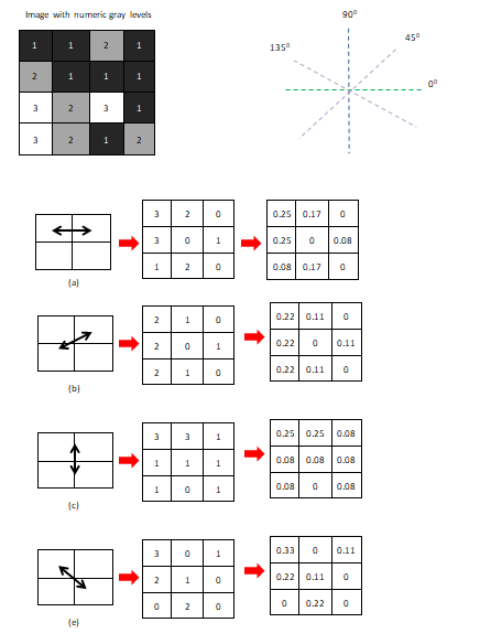
Figure 15: Computing the Haralick texture features from a 4 × 4 example image step by step

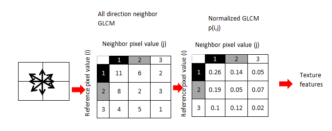
Figure 16: Computing the Haralick texture features from a 4 × 4 example image with all direction

3.3 Color Features

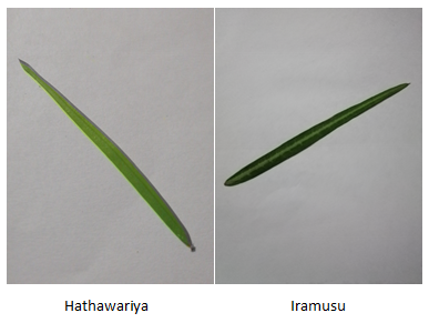
Figure 17: Images of plant species Hathawariya and Iramusu.

Color is an important characteristic of images (Wäldchen and Mäder, 2018; Caglayan et al., 2013). Some of the leaf images have very similar shapes like Hathawariya (Figure 17) and Iramusu (Figure 17). Even though shapes are similar in some leaves, there are some differences in the colors of leaf images. Therefore in addition to the shape features, we extract features related to the color. The colors of an image are formed based on Red-Green-Blue (RGB) colour channels of an image. Color properties are defined within a particular color channel (Kodituwakku and Selvarajah, 2004; Wäldchen and Mäder, 2018). In the field of image recognition, several general color descriptors have been introduced. Color moments (Kodituwakku and Selvarajah, 2004; Wäldchen and Mäder, 2018) are the simple descriptor among them. Mean, standard deviation skewness, and kurtosis are the common moments. Color moments are convenient for real-time applications due to their low dimension and low computational complexity.

We used mean ($M$) and standard deviation ($SD$) of intensity values of red, green and blue channels as color features. Let $h$ be the number of pixels of the image and $r$ is the channel type which can be red, green, or blue. The corresponding colour features are calculates as follows:

$$M=\frac{\text{Total insensity value of }r^{th}\text{channel of the image pixels}}{\text{Total intensity value of the image}},$$ (5)

$$SD=\frac{\sqrt{\sum_{j=0}^{h}(r^{th}\text{channel intensity}_{j}-r^{th}\text{mean value})^{2}}}{\text{Total intensity value of the image}}.$$ (6)

3.4 Scagnostic features

Scagnostic features are used to quantify the characteristics of 2D scatterplot diagrams (Wilkinson and Wills, 2008). Scagnostic measures are calculated based on the appearance of the scatterplot. All the scagnostics features are calculated by using the R package called binostics. Scagnostic features have the range of [0,1]. There are 9 measures that are classified into three categories as shown in Figure 18. Based on binary images, scagnostic features are extracted. To the best of our knowledge, this is the first time, the scagnostic features are used for image recognition.

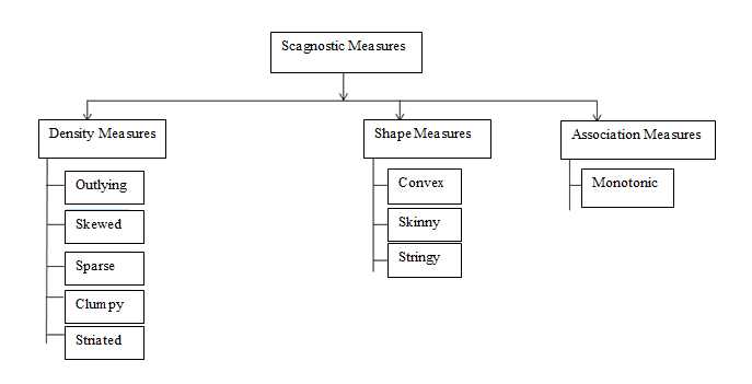
Figure 18: Hierarchy of Scagnostics

We separately measure the scagnostic features based on the cartesian and polar coordinates of the contour (see Figure 19). As the first step, we have to extract the contour of the leaf image (see Figure 19). Then find the $x$ and $y$ coordinate values of the cartesian and polar separately. The $x$ and $y$ coordinate values are used to calculate the scagnostic features. The following definitions can be useful in understanding scagnostics features.

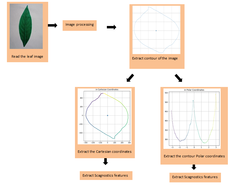
Figure 19: Preprocessing for Scagnostics

Geometric Graphs

1. Graph: A graph $Gr=(Ve,Ed)$ is defined as a set of vertices ($Ve$) together with a relation on $Ve$ induced by a set of edges ($Ed$). A pair of vertices is defined as an edge $e(\nu,\omega)$, with e $\in$ Ed and $\nu,\omega\in$ Ve.

2. Geometric Graph: A geometric graph $G*=[f(Ve),g(Ed),S]$; is an mapping of vertices to points and edges to straight lines to connect points in a metric space $S$.

1. Length of an edge: The Euclidean distance between vertices that are connected to an edge is defined as the length of an edge, $length(e)$.

2. Length of a graph: The sum of the lengths of edges in a graph is known as the length of a graph, $length(Gr)$.

3. Path: A list of successively adjacent, distinct edges are known as a path. If the first and last vertices coincide, then the path is closed.

4. Polygon: A region bounded by a closed path is known as a polygon ($P$). A polygon bounded by exactly one closed path with no intersecting edges is known as a simple polygon.

5. The perimeter of a simple polygon: The length of the boundary of a simple polygon is known as the perimeter of a simple polygon. The area of the interior of a simple polygon is known as the area of a simple polygon.

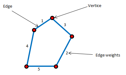
(a) Graph with 5 vertices and 5 edges

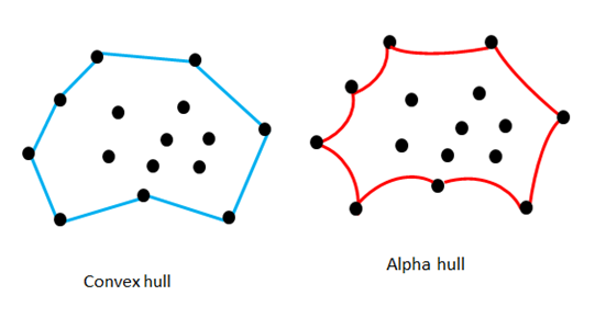
(b) Convex hull and alpha hull

Figure 20: Illustration of vertices, edges, convex hull, and alpha hull

The calculation of scagnostic features require identification of the minimum spanning tree, convex hull, and alpha hull.

Minimum Spanning Tree:

The spanning tree of the graph is defined as $G^{\prime}(V^{\prime},E^{\prime})$, where $V^{\prime}=Ve$, $E^{\prime}\subset Ed$ and $E^{\prime}=|Ve|-1$. A graph can have more than one spanning tree. The spanning-tree should not be disconnected and should not contain any cycles. A spanning tree whose total length is least of all spanning trees on a given set of points is known as a Minimum Spanning Tree (MST).

Convex hull and Alpha hull

1. Convex Hull (see Figure 20(b)): Given a set of points embedded in 2D Euclidean space, the convex hull of the set is the smallest convex polygon that contains all its points.

1. Alpha Hull (see Figure 20(b)): The alpha hull is a generalization of the convex hull. It is defined as the union of all convex hulls of the input within balls of radius alpha. In other words, it is a set of piecewise linear simple curves in the Euclidean plane associated with a given set of points in the 2D Euclidean space. An open disk ($D(r)$) with radius $r$ is used to define the indicator function to identify the associated points. If a point is on the boundary of $D$ then $D$ touches a point and if a point is inside $D$ then $D$ contains a point.

3.4.1 Preprocessing steps related to scagnostic features

To improve the performance of the algorithm and robustness of the measures, preprocessing techniques such as binning and deleting outliers are used before computing geometric graphs related features.

1. Binning

As the first step of binning, the data are normalized to the unit interval. Then use a $40\times 40$ hexagonal grid to aggregate the points in each scatterplot. We reduce the bin size by half and rebind until no more than 250 non-empty cells. If there are more than 250 non-empty cells. When selecting the bins two important points to consider are: i) efficiency (too many bins slow down calculations of the geometric graphs) and ii) sensitivity (fewer bins obscure features in the scatterplots). To improve the performance, hexagon binning is used. To manage the problem of having too many points that start to overlap, hexagon binning is used. The plots of hexagonal binning are density rather than points. There are several reasons for using hexagon binning instead of square binning on a 2D surface. Hexagons are more similar to circles than squares. To keep scagnostics orientation-independent this bias reduction is important.

The weight function is defined as

$$\text{weight}=0.7+\frac{0.3}{1+t^{2}},$$ (7)

where $t=\frac{n}{500}$ ($n$ is the number of vertex).

If $n>2000$ then this function is fairly constant. By using hex binning the shape and the parameters of the function are determined. In computing sparse, skewed, and convex scagnostics this weight function is used to adjust for bias.

1. Deleting Outliers

To improve the robustness of the scagnostics, deleting outliers can be used. A vertex whose adjacent edges in the MST all have a weight (length) greater than $\omega$ is defined as an outlier in this context. By considering nonparametric criteria for the simplicity and Tukey’s idea choose the following weight calculation is

$$\text{weight}=qu_{75}+1.5(qu_{75}-qu_{25}),$$ (8)

where $qu_{75}$ is the 75th percentile of the MST edge lengths and $(qu_{75}-qu_{25})$ is the interquartile range of the edge lengths.

1. Degree of a Vertex

The degree of a vertex in an undirected graph is the number of edges associated with the vertex. For example, vertices of degree 5 means there are 5 edges associated with each vertex (see Figure 20(a)).

3.4.2 Definitions of Scagnostic Features

The definitions of scagnostic features are defined as follows. Our notations are as follows: i) Convex hull ($CH$), ii) Alpha hull ($Al$) and iii) Minimum spanning tree ($MST$). In the following section, we give a brief description of the calculation of scagnostic measures. For more details on rotation techniques, see Wilkinson and Wills (2008).

3.4.3 Density Measures

1. Outlying: The outlying measure is calculated before deleting the outliers for the other measures. The outlying measure is

$$F_{sc1}=\frac{\text{Total length of edges adjacent to outlying points}}{\text{Total edge length of the MST}}.$$ (9)

1. Skewed: The skewed measure is the first measure of relative density, a relatively robust measure of skewness in the distribution of edge lengths. After adaptive binning skewed tends to decrease with $n$. The skewed measure is calculated using the equations

$$F_{sc2}=1-\text{weight}*(1-qu_{skew}),$$ (10)

where,

$$qu_{skew}=\frac{qu_{90}-qu_{50}}{qu_{90}-qu_{10}},$$ (11)

and the calculation of $weight$ is given in equation 7.

1. Sparse: The second relative density measure is a sparse measure that measures whether points in a 2D scatterplot are confined to a lattice or a small number of locations on the plane. The sparse is measured by

$$F_{sc3}=\text{weight}*qu_{90},$$ (12)

where the weight function is equation 7 and $qu_{90}$ is the 90th percentile of the distribution of edge lengths in the $MST$.

1. Clumpy: Clumpiness measures the number of small-scale structures in the 2D-scatter plot (Wilkinson and Wills 2008). In order to calculate this feature another measurement called $T$ is needed which is calculated based on the RUNT graph (Hartigan and Mohanty, 1992). The clumpy is measured by

$$F_{sc4}=max_{j}[1-\frac{max_{k}[length(e_{k})]}{length(e_{j})}].$$ (13)

In the formula below the $j$ value goes over the edges in $MST$ and $k$ runs over all edges in the RUNT graph.

1. Striated: Striated define the coherence in a set of points as the presence of relatively smooth paths in the minimum spanning tree. This measure is based on the number of adjacent edges whose cosine is less than minus 0.75. The stratified is measured by

$$F_{sc5}=\frac{1}{|Ve|}\sum_{\nu\in Ve^{(2)}}I(\cos\theta_{e(\nu,a)e(\nu,b)}<-0.75),$$ (14)

where $Ve^{(2)}\subseteq Ve$ and $I()$ be an indicator function.

3.4.4 Scagnostic-based Shape Measures

Both topological and geometric aspects of the shape of a set of scattered points is considered. As an example, a set of scattered points on the plane appeared to be connected, convex, and so forth, want to know under the shape measures. By definition scattered points are not like this. Therefore to make inferences additional machinery (based on geometric graphs) is needed. By measuring the aspects of the convex hull, the alpha hull, and the minimum spanning tree is determined.

1. Convex: The ratio of the area of the alpha hall ($Al$) and the area of the convex hull ($CH$) is the base of measuring convexity. The convex is measured by

$$F_{sc6}=\text{weight}\times\frac{\text{Area of alpha hull}}{\text{Area of convex hull}},$$ (15)

where the weight function is equation 7.

1. Skinny: Skinny is measured by using the corrected and normalized ratio of perimeter to the area of polygon measures. The skinny is measured by

$$F_{sc7}=1-\frac{\sqrt{4\times\pi\times\text{Area of alpha hull}}}{\text{Perimeter of alpha hull}}.$$ (16)

Furthermore

$$F_{sc7}=\Bigg{\{}^{0;\text{ if circle}}_{\text{Near }1;\text{ if skinny}.}$$

1. Stringy: A skinny shape with no branches is known as a stringy shape. By counting the vertices of degree 2 in the minimum spanning tree and comparing them to the overall number of vertices minus the number of single-degree vertices, a skinny measure is calculated. To adjust for negative skew in its conditional distribution of $n$, cube the stringy measure. The stringy is measured by

$$F_{sc8}=\frac{|Ve^{(2)}|}{|Ve|-|Ve^{(1)}|},$$ (17)

where $Ve$ is the number of vertices.

3.4.5 Association Measure

Symmetric and relatively robust measures of the association are interested. To assess the monotonicity in a scatter plot, the squared Spearman correlation coefficient is used. In calculating monotonicity, the squared value of the coefficient is considered to remove the distinction between positive and negative coefficients. The reason is, the researchers are more interested in how strong the relationship is rather than their direction (negative or positive).

3.4.6 Number of Minimum ($F_{8}$) and Maximum Points ($F_{9}$)

Number of minimum, and maximum points are new measures that are obtained from the polar coordinate of leaf contour. The number of global maximum points ($F_{8}$) and the number of global minimum points ($F_{9}$) are also considered as features.

3.4.7 Correlation of Cartesian Contour ($F_{10}$)

Correlation is another new feature computed based on the cartesian contour. The measure is calculated as

$$F_{10}=\frac{\sum_{i=0}^{m}(x_{i}-\overline{\rm x})(y_{i}-\overline{\rm y})}{\sqrt{\sum_{i=0}^{m}(x_{i}-\overline{\rm x})^{2}(y_{i}-\overline{\rm y})^{2}}},$$ (18)

where $(x_{i},y_{i})$ is the coordinate of cartesian contour and $m$ is the number of points in the cartesian contour

4 Empirical Application

4.1 Data sets

We use two publicly available datasets to demonstrate the applications of features. They are i) Flavia leaf image dataset and ii) Swedish leaf image dataset

4.1.1 Flavia Leaf Image Dataset

The Flavia dataset contains 1907 leaf images. There are 32 different species and each has 50-77 images. Scanners and digital cameras are used to acquire the leaf images on a plain background. The isolated leaf images contain blades only, without a petiole. These leaf images are collected from the most common plants in Yangtze, Delta, China (Wäldchen and Mäder, 2018). Those leaves were sampled on the campus of the Nanjing University and the Sun Yat-Sen arboretum, Nanking, China (Wäldchen and Mäder, 2018) available at https://sourceforge.net/projects/flavia/files/Leaf%2520Image%2520Dataset/.

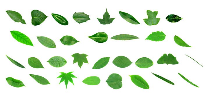
(a) Sample of Flavia dataset

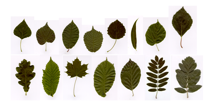
(b) Sample of Swedish leaf dataset

Figure 21: Samples from Flavia and Swedish datasets

4.1.2 Swedish Leaf Image Dataset

The Swedish dataset contains 1125 images. The images of isolated leaf scans on a plain background of 15 Swedish tree species, with 75 leaves per species. This dataset has been captured as part of a joined leaf classification project between the Linkoping University and the Swedish Museum of Natural History (Wäldchen and Mäder, 2018) available at https://www.cvl.isy.liu.se/en/research/datasets/swedish-leaf/.

We applied the aforementioned image processing techniques and computed features from each image.

4.2 Visualization of ability of features to distinguish classes of interest

In order to identify the ability of features to distinguish classes of interest, we first label features according to their shapes as i) diamond, ii) heart shape, iii) needle shape, iv) simple round, and v) round shape (see Figure 2(b)). These morphological characteristics are identified by observing images in the medicinal plant repository maintained by Barberyn Ayurveda resort and University of Ruhuna available at http://www.instituteofayurveda.org/plants/. Our observed results are converted into an open-source R software package called MedLEA: Medicinal LEAf which is available on Comprehensive R Archive Network (Lakshika and Talagala, 2021).

We explore the ability of features to classify images under supervised learning settings and unsupervised learning settings. For this purpose, we use Linear Discriminant Analysis (LDA) and Principal Component Analysis (PCA). LDA is a supervised dimensionality reduction technique, and PCA is an unsupervised dimensionality reduction technique. In this section, we visualize and compare the results obtained using LDA, and PCA on Flavia and Swedish datasets. To compute the LDA projection shape label is taken as the response variable. There are 5 main shape categories as: diamond, simple round, round, needle, and heart shape.

We further explore the ability of our features to classify classes when there is a moderately large number of class labels. For that, we label the leaves according to their species type. In the Swedish data set, there are 12 species-wise class categories while the Flavia data set contains 32 species-wise class categories. Both PCA and LDA approaches were used to explore the class separability visually. To explore the class separability of species in the PCA space, we colour the points according to their species labels. For the corresponding LDA analysis, we use species class labels as the response variable.

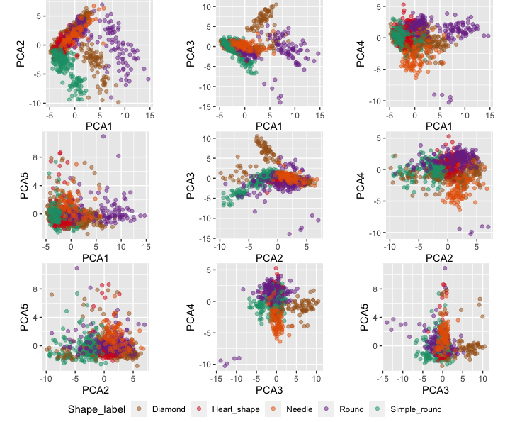
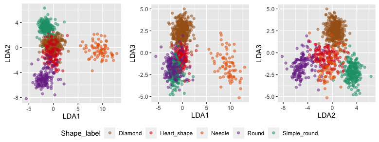
Figure 22: Distribution of Swedish leaf images on the principal component analysis-based projection space. All projected points are coloured according to their shape labels.

Figure 23: Distribution of Swedish leaf images on linear discriminant analysis based projection space. All projected points are coloured according to their shape labels.

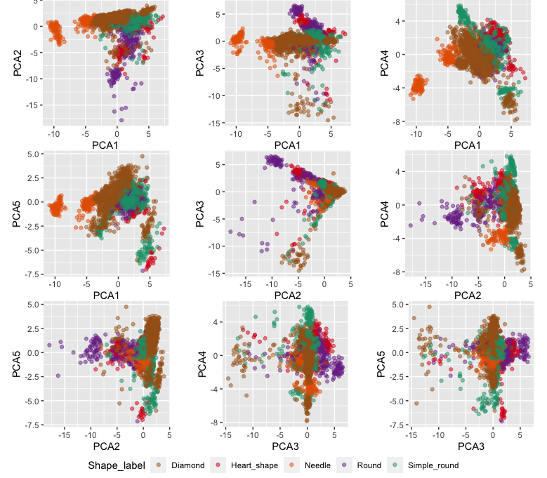
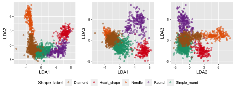
Figure 24: Distribution of Flavia leaf images on the principal component analysis based projection space. All projected points are coloured according to their shape labels.

Figure 25: Distribution of Flavia leaf images on linear discriminant analysis based projection space. All projected points are coloured according to their shape labels.

Feature name	Swedish								Flavia
	PCA1	PCA2	PCA3	PCA4	PCA5	LDA1	LDA2	LDA3	PCA1	PCA2	PCA3	PCA4	PCA5	LDA1	LDA2	LDA3
Skewed polar	0.05	-0.08	-0.11	-0.03	0.03	1.48	-0.49	-0.17	0.02	-0.03	-0.10	0.09	-0.02	0.01	1.96	0.60
Clumpy polar	0.04	-0.07	-0.07	-0.01	-0.03	5.65	2.42	-5.47	-0.02	-0.03	-0.06	-0.01	-0.02	-1.46	1.25	1.85
Sparse polar	0.10	-0.21	-0.16	-0.07	-0.05	-19.55	-9.32	52.97	0.02	-0.15	-0.29	0.02	0.00	-35.36	3.04	44.68
Striated polar	-0.13	0.22	0.21	0.01	-0.02	-1.08	-0.97	5.32	-0.05	0.14	0.31	-0.07	0.01	1.79	0.24	0.43
Convex polar	0.12	-0.21	-0.18	-0.06	-0.03	0.44	6.59	3.54	0.04	-0.16	-0.32	0.03	0.03	11.76	-20.21	4.70
Skinny polar	0.01	-0.09	-0.04	-0.02	0.08	0.67	0.06	0.19	-0.01	-0.02	-0.08	0.05	0.00	0.13	0.04	-0.12
Stringy polar	-0.15	0.14	0.19	-0.01	-0.10	-4.10	4.80	-1.99	-0.05	0.15	0.28	-0.07	0.01	-3.44	-3.07	8.62
Monotonic polar	0.09	0.02	-0.05	0.14	0.17	-1.51	-2.54	1.34	0.07	0.06	0.05	-0.09	0.18	0.14	0.34	-1.71
Skewed contour	0.07	-0.16	-0.15	0.01	0.03	-1.99	-2.33	-2.28	0.01	-0.04	-0.09	-0.05	-0.06	-0.39	0.10	-2.35
Clumpy contour	0.04	-0.05	-0.08	0.05	0.05	-8.59	3.43	-0.49	0.02	-0.02	-0.04	-0.01	0.00	-1.07	-2.38	1.29
Sparse contour	0.16	-0.18	-0.17	-0.02	0.01	54.36	45.24	34.38	0.02	-0.16	-0.29	0.00	0.02	-29.91	7.74	-114.90
Striated contour	-0.15	0.21	0.20	0.00	-0.02	4.19	0.70	2.59	-0.04	0.15	0.31	0.01	0.02	-0.11	0.24	-4.12
Convex contour	0.12	-0.21	-0.17	-0.05	-0.03	4.92	-8.62	8.77	0.04	0.015	-0.05	0.09	0.10	-0.43	2.56	0.89
Skinny contour	0.04	-0.10	-0.07	0.04	0.03	0.63	0.24	-0.34	-0.03	0.00	-0.13	-0.11	0.04	0.13	0.67	-0.20
Stringy contour	-0.13	0.08	0.13	-0.02	-0.09	-1.68	-4.53	-4.57	-0.04	0.15	0.30	-0.01	-0.03	-1.63	0.34	0.29
Monotonic contour	0.01	0.04	0.01	-0.17	0.07	6.63	-1.24	-3.58	0.05	0.03	0.08	0.25	0.05	0.25	0.57	-0.21
No of max points	0.08	-0.22	-0.20	0.00	-0.04	0.00	-0.08	-0.02	-0.02	-0.15	-0.23	0.05	-0.03	0.06	0.04	-0.06
No of min points	0.07	-0.21	-0.18	-0.01	-0.06	-0.05	0.07	-0.01	-0.02	-0.16	-0.22	-0.12	-0.04	0.01	0.00	0.14
diameter	0.01	-0.08	0.11	0.45	-0.12	0.05	-0.03	-0.04	-0.03	0.15	-0.08	-0.28	0.29	0.02	0.02	0.02
area	-0.19	-0.21	0.05	0.16	-0.07	-0.00	0.00	0.00	0.28	0.04	0.00	-0.01	0.15	0.00	0.00	-0.00
perimeter	0.09	-0.20	0.29	0.11	-0.03	-0.01	-0.00	-0.00	0.12	-0.16	0.09	-0.23	0.28	0.01	0.00	-0.01
physiological length	0.00	-0.07	0.10	0.47	-0.13	-0.01	0.01	0.05	-0.05	0.16	-0.09	-0.27	0.30	-0.04	-0.03	0.00
physiological width	-0.14	-0.25	0.16	0.00	-0.07	0.05	0.01	0.02	0.27	-0.13	0.09	0.05	0.05	-0.04	-0.02	0.02
aspect ratio	-0.14	-0.21	0.11	-0.24	-0.01	-31.15	0.92	5.74	0.22	-0.18	0.11	0.11	-0.07	-0.87	-12.64	-14.56
rectangularity	-0.15	0.05	-0.21	-0.05	0.11	39.81	-9.31	-54.21	-0.03	0.25	-0.13	0.10	-0.11	-14.56	-1.64	33.27
circularity	-0.25	0.02	-0.20	0.02	-0.02	-46.07	-23.83	20.01	0.24	0.13	-0.05	0.18	-0.06	-2.94	-2.04	9.07
compactness	0.23	-0.06	0.23	-0.01	0.03	0.14	0.48	-0.61	-0.22	-0.07	0.03	-0.18	-0.02	0.20	-0.09	0.05
NF	0.16	0.20	-0.12	0.20	0.02	-16.21	6.44	10.63	-0.24	0.01	-0.02	-0.17	-0.03	-3.10	4.49	1.31
Perimeter ratio diameter	0.10	-0.18	0.28	-0.16	0.04	2.36	-5.70	-7.27	0.11	-0.29	0.16	0.05	-0.02	4.53	4.16	2.34
Perimeter ratio length	0.25	0.10	0.04	0.12	0.05	3.18	-2.18	-3.87	-0.23	0.00	-0.01	-0.17	-0.03	1.75	-1.91	-0.73
Perimeter ratio lw	0.21	-0.08	0.22	-0.08	0.08	16.86	2.38	54.00	-0.13	-0.26	0.12	-0.12	0.01	-37.98	-19.58	-5.38
No of Convex points	-0.20	-0.01	0.05	-0.12	0.05	0.08	-0.01	0.07	0.06	0.20	-0.12	0.11	0.02	0.00	0.02	-0.01
perimeter convexity	-0.18	0.12	-0.26	0.10	-0.03	63.15	21.37	3.69	-0.04	0.31	-0.16	0.04	-0.04	-6.46	-48.53	-60.23
area convexity	0.23	-0.08	0.19	0.02	0.04	-7.31	-17.58	39.50	-0.04	-0.31	-0.31	-0.09	0.03	-4.75	-5.18	-10.42
area ratio convexity	-0.24	0.08	-0.19	-0.03	-0.04	23.67	12.15	74.99	0.04	0.31	-0.16	0.09	-0.03	-16.03	-30.33	-40.54
equivalent diameter	-0.18	-0.20	0.08	0.19	-0.08	-0.03	0.03	-0.02	0.29	0.04	0.00	0.01	0.15	0.03	0.00	-0.01
cx	-0.06	-0.05	-0.04	0.12	0.00	-0.00	0.00	0.00	-0.03	0.10	-0.05	0.01	0.07	0.00	0.00	0.00
cy	-0.16	-0.17	0.05	-0.12	0.03	0.01	0.01	-0.01	0.01	0.05	0.00	-0.04	0.09	0.00	0.00	0.00
eccentricity	0.09	0.20	-0.17	0.24	-0.01	-11.57	-1.28	-1.46	-0.15	0.22	-0.13	-0.10	0.07	0.02	4.63	5.11
contrast	-0.18	-0.05	0.03	-0.11	-0.04	-0.01	0.01	0.04	0.12	0.07	-0.03	-0.19	0.19	0.01	-0.00	0.00
correlation texture	0.15	0.02	-0.02	0.18	0.05	-0.04	-74.65	653.77	-0.02	-0.01	0.02	0.26	-0.18	162.60	70.64	89.69
inverse difference moments	0.18	0.17	-0.02	-0.01	0.27	-0.50	1.33	-6.73	-0.28	-0.041	0.01	0.06	-0.19	-3.13	13.77	13.95
entropy	-0.17	-0.18	-0.01	0.12	-0.26	-0.25	-0.07	-0.14	0.28	0.05	-0.01	-0.06	0.18	0.14	1.26	1.41
Mean Red value	0.13	0.11	-0.02	-0.03	-0.43	-0.01	0.00	0.01	0.17	0.06	0.00	-0.24	-0.34	-0.02	-0.03	0.03
Mean Green value	0.17	0.17	-0.02	-0.21	-0.16	0.00	0.03	-0.02	0.23	0.06	0.00	-0.20	-0.24	-0.01	0.03	-0.02
Mean Blue value	0.13	0.13	-0.03	-0.10	-0.42	0.01	0.00	0.01	0.19	0.06	0.00	-0.24	-0.31	0.02	0.00	0.01
SD Red value	0.04	0.04	0.00	-0.12	-0.44	0.01	-0.02	-0.02	0.16	0.06	0.00	-0.26	-0.32	0.00	-0.04	-0.03
SD Green value	-0.15	-0.03	0.04	0.19	0.24	0.02	-0.05	-0.02	0.19	-0.03	0.02	0.06	0.20	0.00	-0.01	0.01
SD Blue values	-0.09	0.00	0.05	-0.07	0.24	0.00	-0.02	0.02	0.21	0.05	0.00	-0.25	-0.21	0.01	0.06	0.00
correlation	0.00	0.01	0.00	-0.05	0.08	0.16	-0.13	0.58	0.03	0.10	0.03	0.23	0.02	-0.04	-0.23	0.21
Cummulative proportion - PCA	0.24	0.43	0.54	0.61	0.66				0.21	0.36	0.49	0.58	0.64

Table 4: Summary of PCA & LDA coefficients (shape-wise classification)

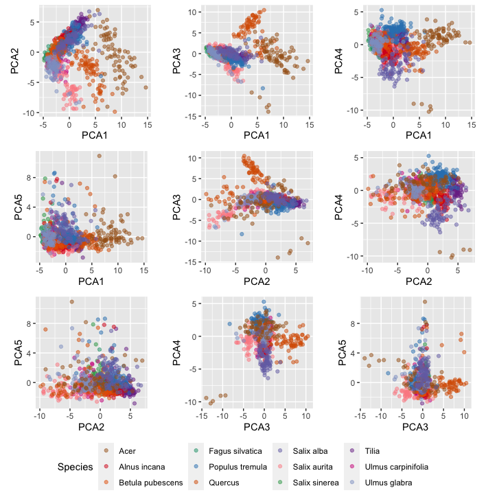
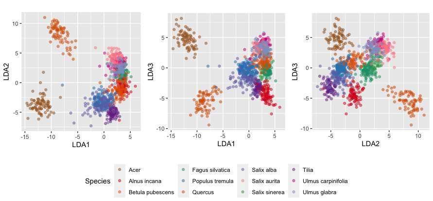
Figure 26: Distribution of Swedish leaf images on the principal component analysis-based projection space. All projected points are coloured according to their species labels.

Figure 27: Distribution of Swedish leaf images on linear discriminant analysis based projection space. All projected points are coloured according to their species labels.

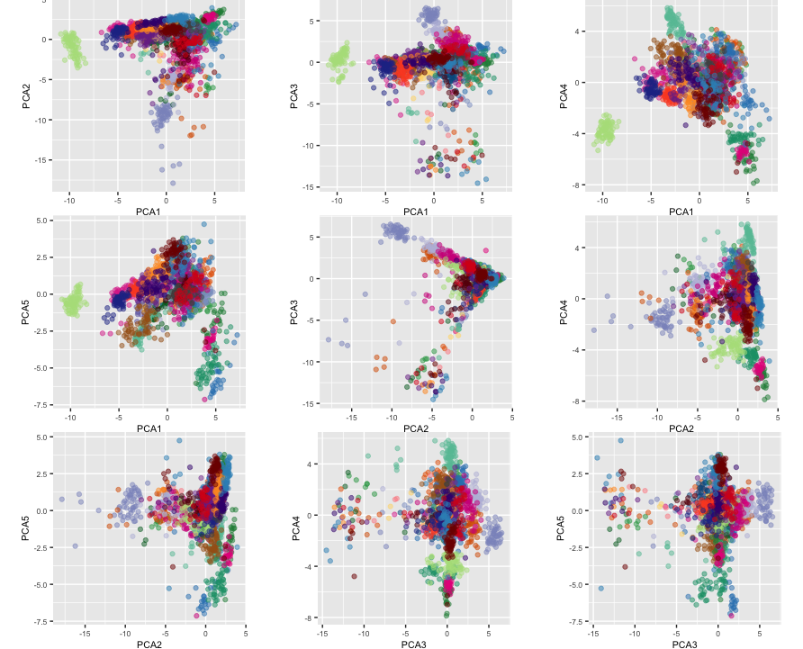
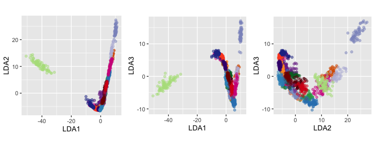
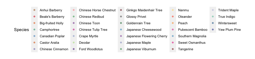
Figure 28: Distribution of Flavia leaf images on the principal component analysis-based projection space. All projected points are coloured according to their species labels.

Figure 29: Distribution of Flavia leaf images on linear discriminant analysis based projection space. All projected points are coloured according to their species labels.

Feature Name	Swedish								Flavia
	PCA1	PCA2	PCA3	PCA4	PCA5	LDA1	LDA2	LDA3	PCA1	PCA2	PCA3	PCA4	PCA5	LDA1	LDA2	LDA3
Skewed polar	0.05	-0.08	-0.11	-0.03	0.03	1.16	-0.03	-2.37	0.02	-0.03	-0.10	0.09	-0.02	1.02	-0.42	1.00
Clumpy polar	0.04	-0.07	-0.07	-0.01	-0.03	0.86	0.09	0.20	-0.02	-0.03	-0.06	-0.01	-0.02	3.05	1.59	-1.89
Sparse polar	0.10	-0.21	-0.16	-0.07	-0.05	-45.51	88.66	-115.87	0.02	-0.15	-0.29	0.02	0.00	-31.04	-5.91	-20.03
Striated polar	-0.13	0.22	0.21	0.01	-0.02	-2.37	-0.94	-3.69	-0.05	0.14	0.31	-0.07	0.01	1.88	0.09	-0.39
Convex polar	0.12	-0.21	-0.18	-0.06	-0.03	19.81	-30.88	21.25	0.04	-0.16	-0.32	0.03	0.03	-4.90	-1.27	-1.68
Skinny polar	0.01	-0.09	-0.04	-0.02	0.08	-0.71	-0.03	-0.45	-0.01	-0.02	-0.08	0.05	0.00	-0.02	-0.12	-0.01
Stringy polar	-0.15	0.14	0.19	-0.01	-0.10	7.21	4.40	-1.40	-0.05	0.15	0.28	-0.07	0.01	2.70	1.67	0.13
Monotonic polar	0.09	0.02	-0.05	0.14	0.17	-1.09	-1.49	0.08	0.07	0.06	0.05	-0.09	0.18	0.63	0.51	1.28
Skewed contour	0.07	-0.16	-0.15	0.01	0.03	-0.49	0.21	1.88	0.01	-0.04	-0.09	-0.04	-0.06	-0.36	1.07	1.10
Clumpy contour	0.04	-0.05	-0.08	0.05	0.05	1.50	2.49	8.76	0.02	-0.02	-0.04	-0.01	0.00	-2.03	0.41	2.33
Sparse contour	0.16	-0.18	-0.169	-0.02	0.01	-27.87	0.52	24.01	0.02	-0.16	-0.29	0.00	0.02	11.62	50.00	30.38
Striated contour	-0.15	0.21	0.20	0.00	-0.02	-0.31	1.36	-1.52	-0.04	0.15	0.31	0.01	0.02	-0.07	2.72	1.60
Convex contour	0.12	-0.27	-0.17	-0.05	-0.03	-1.93	24.62	-44.83	0.04	0.01	-0.05	0.09	0.10	0.82	-0.12	2.21
Skinny contour	0.04	-0.10	-0.07	0.04	0.03	0.55	0.57	-0.33	-0.03	0.00	-0.13	-0.12	0.04	0.23	0.35	-0.34
Stringy contour	-0.13	0.08	0.13	-0.02	-0.09	0.83	-0.75	0.52	-0.04	0.15	0.30	-0.01	-0.03	-2.74	-4.56	-2.41
Monotonic contour	0.01	0.04	0.01	-0.17	0.07	-0.96	0.15	0.56	0.05	0.03	0.08	0.25	0.05	-0.04	-0.16	-1.62
No of max points	0.08	-0.21	-0.20	0.00	-0.04	0.02	0.05	0.05	-0.02	-0.15	-0.23	-0.07	-0.03	-0.02	-0.06	0.00
No of min points	0.07	-0.21	-0.18	-0.01	-0.06	-0.01	0.00	0.02	-0.02	-0.16	-0.22	-0.12	-0.03	0.01	0.05	-0.05
diameter	0.01	-0.08	0.11	0.45	-0.12	-0.04	-0.02	-0.02	-0.03	0.15	-0.09	-0.29	0.29	0.03	0.00	-0.01
area	-0.19	-0.21	0.05	0.16	-0.07	0.00	0.00	0.00	0.28	0.04	0.00	-0.01	0.15	0.00	0.00	0.00
perimeter	0.09	-0.20	0.29	0.11	-0.03	0.00	0.00	0.00	0.12	-0.16	0.09	-0.23	0.28	0.00	0.01	0.00
physiological length	0.00	-0.07	0.10	0.47	-0.13	0.01	0.02	-0.02	-0.05	0.16	-0.09	-0.27	0.30	-0.03	-0.04	1.22
physiological width	-0.14	-0.25	0.16	0.00	-0.07	-0.03	0.05	-0.02	0.27	-0.13	0.09	0.05	0.05	-0.03	-0.04	-3.57
aspect ratio	-0.14	-0.21	0.12	-0.24	-0.01	17.34	-11.17	14.83	0.22	-0.18	0.11	0.12	-0.07	-10.67	8.97	9.08
rectangularity	-0.15	0.05	-0.21	-0.05	0.11	1.17	3.71	-29.06	-0.03	0.25	-0.13	0.10	-0.12	-42.29	-3.09	-32.86
circularity	-0.25	0.02	-0.20	0.02	-0.02	-32.21	38.61	21.19	0.24	0.13	-0.05	0.18	-0.06	39.73	-49.27	-0.73
compactness	0.23	-0.06	0.23	-0.01	0.03	82.91	-0.24	-0.12	-0.22	-0.07	0.03	-0.18	-0.02	-0.09	0.05	-0.07
NF	0.16	0.20	-0.12	0.20	0.02	1.21	19.88	-1.71	-0.24	0.01	-0.02	-0.17	-0.03	3.10	-2.01	2.17
Perimeter ratio diameter	0.10	-0.18	0.28	-0.16	0.04	-10.11	6.76	-6.66	0.12	-0.29	0.16	0.05	-0.02	6.48	-0.09	0.48
Perimeter ratio length	0.25	0.10	0.04	0.12	0.05	-1.97	-4.69	5.32	-0.23	0.00	-0.01	-0.17	-0.03	-0.91	1.03	-0.74
Perimeter ratio lw	0.21	-0.08	0.22	-0.08	0.08	-19.35	-0.07	-1.01	-0.13	-0.26	0.12	-0.12	0.01	2.40	-48.35	19.77
No of Convex points	-0.20	-0.01	0.05	-0.12	0.05	0.01	0.02	-0.04	0.06	0.20	0.12	0.11	0.02	-0.03	-0.03	0.06
perimeter convexity	-0.18	0.12	-0.26	0.10	-0.03	30.96	-89.46	-25.06	-0.04	0.31	-0.16	0.05	-0.04	-55.44	-10.72	28.83
area convexity	0.23	-0.08	0.19	0.02	0.04	32.73	-15.20	24.97	-0.04	-0.31	0.16	-0.09	0.03	16.76	-4.85	20.29
area ratio convexity	-0.24	0.078	-0.19	-0.03	-0.04	95.81	-29.35	1.23	0.04	0.31	-0.16	0.09	-0.03	14.55	-1.34	41.66
equivalent diameter	-0.18	-0.20	0.081	0.19	-0.08	0.09	-0.04	0.05	0.29	0.04	0.00	0.01	0.15	0.02	0.08	0.00
cx	-0.06	-0.05	-0.04	0.12	-0.01	0.00	0.00	0.00	-0.03	0.10	-0.05	0.01	0.07	0.00	0.00	0.00
cy	-0.16	-0.17	0.05	-0.12	0.03	0.00	0.00	0.01	0.10	0.05	0.00	-0.04	0.09	0.00	0.00	0.00
eccentriciry	0.09	0.20	-0.17	0.24	-0.01	1.26	3.10	5.13	-0.15	0.22	-0.13	-0.10	0.07	5.37	1.57	-2.01
contrast	-0.18	-0.05	0.03	-0.11	-0.04	-0.09	-0.03	0.05	0.12	0.07	-0.03	-0.19	0.19	0.01	0.02	0.04
correlation texture	0.15	0.02	-0.02	0.18	0.05	-185.14	-233.28	143.05	-0.02	-0.01	0.02	0.26	-0.18	50.17	375.80	296.79
inverse difference moments	0.18	0.17	-0.02	-0.01	0.27	-17.60	-1.87	31.96	-0.28	-0.04	0.01	0.06	-0.19	-7.20	-1.70	39.29
entropy	-0.17	-0.18	-0.01	0.12	-0.26	0.01	0.07	2.32	0.28	0.05	-0.01	-0.06	0.18	-0.36	2.47	4.72
Mean red value	0.13	0.11	-0.02	-0.03	-0.43	-0.01	0.00	0.00	0.17	0.06	0.00	-0.24	-0.34	0.02	-0.04	0.11
Mean green value	0.17	0.17	-0.02	-0.21	-0.16	-0.02	0.00	0.03	0.23	0.06	0.00	-0.20	-0.24	0.03	0.00	0.04
Mean blue value	0.13	0.13	-0.03	-0.10	-0.42	-0.01	-0.01	-0.01	0.19	0.06	0.00	-0.24	-0.31	-0.04	0.04	-0.14
SD red value	0.04	0.04	0.00	-0.12	-0.44	0.02	0.00	0.00	0.16	0.06	0.00	-0.26	-0.32	-0.03	-0.05	-0.12
SD blue value	-0.15	-0.03	0.04	0.19	0.24	0.05	-0.02	-0.06	0.19	-0.03	0.02	0.06	0.20	0.00	-0.04	-0.05
SD green value	-0.09	0.00	0.05	-0.07	0.24	-0.01	0.01	-0.02	0.21	0.05	0.00	-0.25	-0.21	0.01	0.07	0.12
correlation	0.00	0.01	0.00	-0.05	0.08	-0.28	0.26	-0.41	0.03	0.10	0.03	0.23	0.02	0.04	-0.12	0.23
Cummulative proportion - PCA	0.24	0.43	0.54	0.61	0.66				0.21	0.36	0.49	0.58	0.64

Table 5: Summary of PCA & LDA coefficients (species-wise classification)

4.2.1 Swedish Dataset

The visualization of PCA projections of the Swedish dataset is shown in Figure 23. The first three principal components (PCs) accounting for approximately 43% of the total variance in the original data, while the first 5 PCs account for 66% of the total variance in the original data. Hence, the first five PCs are plotted against each other to visualize data in the PCA space. The LDA projections of Swedish data are shown in Figure 23. According to the LDA results on the Swedish dataset, LDA1, LDA2, and LDA3 show a clear separation of shapes of leaf images.

4.2.2 Flavia Dataset

The LDA projections of Flavia data are shown in Figure 25. The visualization of PCA projections of the Flavia dataset is shown in Figure 25. The first three principal components (PCs) accounting for approximately 49% of the total variance in the original data, while the first 5 PCs account for 64% of the total variance in the original data. Hence, the first five PCs are plotted against each other to visualize data in the PCA projection space. According to the LDA results on the Flavia dataset, LDA1, LDA2, and LDA3 shows a clear separation of shapes of leaf images. Under both experimental settings, class separation is more clearly on the LDA space than the PCA space. The reason could be LDA is a supervised learning algorithm while PCA space is an unsupervised learning algorithm.

According to both PCA and LDA visualizations on Swedish and Flavia data sets, we can see a clear separation of classes in their corresponding projection spaces. This reveals our features are capable of distinguishing classes under both supervised learning and unsupervised learning settings. The class separations are clearly visible under both small numbers of class labels and a large number of class labels. The PCA and LDA coefficients for shape-wise classification and species-wise classifications are shown in Table 4 and Table 5 respectively.

5 Discussion and Conclusions

In this paper we introduce computer-aided, interpretable features for image recognition. There are four main categories of features that are used to classify leaf images. Many research was based on shape, color, and texture-based image features. In this research paper, we introduce a new feature category called scagnostics for image classification. Other than that correlation of cartesian coordinate, number of convex points, number of minimum and maximum points are introduced as new shape features. We explore the ability of features to discriminate the classes of interest under supervised learning and unsupervised learning settings using principal component analysis and linear discriminant analysis. Under both experimental settings, a clear separation of classes is visible in their projection spaces. In our next paper, we introduce a meta-learning algorithm to classify plant species using the features introduced in this paper. A more detailed look at the most important features and approach of classification plant species will be presented in our next paper. We hope our analysis opens various research agendas in the field of image recognition. Reproducible research code to reproduce the results of this paper and codes to compute features are available here: https://github.com/SMART-Research/leaffeatures_paper.

References

- Wäldchen and Mäder [2018] Jana Wäldchen and Patrick Mäder. Plant species identification using computer vision techniques: A systematic literature review. Archives of Computational Methods in Engineering, 25(2):507–543, 2018.
- Anantrasirichai et al. [2017] Nantheera Anantrasirichai, Sion Hannuna, and Nishan Canagarajah. Automatic leaf extraction from outdoor images. arXiv preprint arXiv:1709.06437, 2017.
- Wu et al. [2007a] Stephen Gang Wu, Forrest Sheng Bao, Eric You Xu, Yu-Xuan Wang, Yi-Fan Chang, and Qiao-Liang Xiang. A leaf recognition algorithm for plant classification using probabilistic neural network. In 2007 IEEE international symposium on signal processing and information technology, pages 11–16. IEEE, 2007a.
- Azlah et al. [2019] Muhammad Azfar Firdaus Azlah, Lee Suan Chua, Fakhrul Razan Rahmad, Farah Izana Abdullah, and Sharifah Rafidah Wan Alwi. Review on techniques for plant leaf classification and recognition. Computers, 8(4):77, 2019.
- Herdiyeni and Wahyuni [2012] Yeni Herdiyeni and Ni Kadek Sri Wahyuni. Mobile application for indonesian medicinal plants identification using fuzzy local binary pattern and fuzzy color histogram. In 2012 International Conference on Advanced Computer Science and Information Systems (ICACSIS), pages 301–306. IEEE, 2012.
- Gonzalez and Woods [2006] Rafael C. Gonzalez and Richard E. Woods. Digital image processing. Prentice-Hall, Inc., 2006.
- Goyal et al. [2018] N. Goyal, Kapil, and N. Kumar. Plant species identification using leaf image retrieval: A study. In 2018 International Conference on Computing, Power and Communication Technologies (GUCON), pages 405–411, 2018.
- Wu et al. [2007b] Stephen Gang Wu, Forrest Sheng Bao, Eric You Xu, Yu-Xuan Wang, Yi-Fan Chang, and Qiao-Liang Xiang. A leaf recognition algorithm for plant classification using probabilistic neural network. In 2007 IEEE International Symposium on Signal Processing and Information Technology, pages 11–16. IEEE, 2007b.
- Söderkvist [2001] Oskar Söderkvist. Computer vision classification of leaves from swedish trees, 2001.
- Mingqiang et al. [2008] Yang Mingqiang, Kpalma Kidiyo, and Ronsin Joseph. A survey of shape feature extraction techniques. Pattern Recognition, 15(7):43–90, 2008.
- Sun et al. [2017] Yu Sun, Yuan Liu, Guan Wang, and Haiyan Zhang. Deep learning for plant identification in natural environment. Computational intelligence and neuroscience, 2017, 2017.
- Wilkinson et al. [2005] Leland Wilkinson, Anushka Anand, and Robert Grossman. Graph-theoretic scagnostics. In IEEE Symposium on Information Visualization (InfoVis 05), pages 157–158. IEEE Computer Society, 2005.
- Dean [1999] C Dean. Quantitative description and automated classification of cellular protein localization patterns in fluorescence microscope images of mammalian cells. PhD thesis, PhD thesis, Carnegie Mellon University, 1999.
- Caglayan et al. [2013] Ali Caglayan, Oguzhan Guclu, and Ahmet Burak Can. A plant recognition approach using shape and color features in leaf images. In International Conference on Image Analysis and Processing, pages 161–170. Springer, 2013.
- Kodituwakku and Selvarajah [2004] Saluka Ranasinghe Kodituwakku and S Selvarajah. Comparison of color features for image retrieval. Indian Journal of Computer Science and Engineering, 1(3):207–211, 2004.
- Wilkinson and Wills [2008] Leland Wilkinson and Graham Wills. Scagnostics distribution. Journal of Computational and Graphical Statistics, 17:473–491, 06 2008. doi:10.1198/106186008X320465.
- Hartigan and Mohanty [1992] John A Hartigan and Surya Mohanty. The runt test for multimodality. Journal of Classification, 9(1):63–70, 1992.
- Lakshika and Talagala [2021] Jayani P. G. Lakshika and Thiyanga S. Talagala. Medlea: Morphological and structural features of medicinal leaves. 2021. URL https://CRAN.R-project.org/package=MedLEA. R package version 1.0.1.
- Aakif and Khan [2015] Aimen Aakif and Muhammad Faisal Khan. Automatic classification of plants based on their leaves. Biosystems Engineering, 139:66–75, 2015.
- Jeon and Rhee [2017] Wang-Su Jeon and Sang-Yong Rhee. Plant leaf recognition using a convolution neural network. International Journal of Fuzzy Logic and Intelligent Systems, 17(1):26–34, 2017.
- Dang and Wilkinson [2014] Tommy Dang and Leland Wilkinson. Scagexplorer: Exploring scatterplots by their scagnostics. pages 73–80, 03 2014. doi:10.1109/PacificVis.2014.42.
- Dang et al. [2012] Tuan Nhon Dang, Anushka Anand, and Leland Wilkinson. Timeseer: Scagnostics for high-dimensional time series. IEEE Transactions on Visualization and Computer Graphics, 19(3):470–483, 2012.
- Kalyoncu and Toygar [2015] Cem Kalyoncu and Önsen Toygar. Geometric leaf classification. Computer Vision and Image Understanding, 133:102–109, 2015.
- Haralick et al. [1973] Robert M Haralick, Karthikeyan Shanmugam, and Its’ Hak Dinstein. Textural features for image classification. IEEE Transactions on systems, man, and cybernetics, (6):610–621, 1973.
- Bangare et al. [2015] Sunil L Bangare, Amruta Dubal, Pallavi S Bangare, and ST Patil. Reviewing otsu’s method for image thresholding. International Journal of Applied Engineering Research, 10(9):21777–21783, 2015.