The EMU view of the Large Magellanic Cloud: Troubles for sub-TeV WIMPs

Abstract

We present a radio search for WIMP dark matter in the Large Magellanic Cloud (LMC). We make use of a recent deep image of the LMC obtained from observations of the Australian Square Kilometre Array Pathfinder (ASKAP), and processed as part of the Evolutionary Map of the Universe (EMU) survey. LMC is an extremely promising target for WIMP searches at radio frequencies because of the large J-factor and the presence of a substantial magnetic field. We detect no evidence for emission arising from WIMP annihilations and derive stringent bounds on the annihilation rate as a function of the WIMP mass, for different annihilation channels. This work excludes the thermal cross section for masses below 480 GeV and annihilation into quarks.

1 Introduction

The nature of dark matter (DM) is one of the defining mysteries of modern physics. One of the most attractive candidates proposed to solve the DM puzzle is given by hypothetical particles that are more massive than baryons and weakly interacting, the so-called WIMPs [1].

WIMPs have masses in the GeV-TeV range and can annihilate in pairs into lighter particles. In particular, electrons and positrons can be directly or indirectly injected by WIMP annihilations, and a sizable final branching ratio of annihilation into $e^{+}-e^{-}$ is a rather generic feature of WIMP models (see, e.g., Fig. 4 in Ref. [2]). Emitted in an environment with a background magnetic field, high-energy electrons and positrons give rise to synchrotron radiation typically peaking at radio frequencies.

The Large Magellanic Cloud (LMC) is the most massive satellite galaxy of the Milky Way. The large dark matter mass (with the LMC virial mass being around $10^{11}\,M_{\odot}$ [3]) and the proximity to Earth (distance around 50 kpc [4]) make the LMC one of the best targets for indirect searches of WIMPs. The so-called J-factor, namely, the integral of the density squared over the line-of-sight and solid angle, amounts to $\sim 10^{20}{\rm GeV^{2}/cm^{5}}$ [5], second only to the Galactic center. The presence in LMC of a $\mu$G magnetic field [6] suggests an investigation of a possible WIMP signature at radio frequencies.

The idea of deriving bounds on WIMPs from radio observations of the LMC is not new [7, 8]. The improvement presented in the current analysis with respect to Refs. [7] and [8] arises from new, more sensitive, data, an updated model (with the inclusion of spatial diffusion in the computation of the DM signal), and the choice of statistical approach (comprising a morphological analysis with pixel by pixel comparison of the observed and predicted signals).

We use observations of the LMC obtained by the Australian Square Kilometre Array Pathfinder (ASKAP [9]), as part of the ASKAP commissioning and early science (ACES, project code AS033) verification and made available to the Evolutionary Map of the Universe (EMU) project [10]. These data were used to obtain a deep image of the LMC at 888 MHz [11], which will be the starting point of the analysis of this work.

The structure of the paper is as follows. Section 2 describes the ASKAP observations and how the LMC radio image has been created. The model of DM and interstellar medium in the LMC is presented in Section 3. We introduce the statistical analysis and present the results in Section 4, while Section 5 provides a comparison with previous works. Conclusions are drawn in Section 6. The Appendix is devoted to consistency checks.

2 Observational Maps

In this work we make use of the observations of the LMC taken as part of the ASKAP commissioning and early science at 888 MHz with a bandwidth of 288 MHz, and analysed as part of the EMU project [11]. The observations cover a total field of view of 120 deg², with a total exposure time of about 12h40m. Data processing was performed using ASKAPsoft by the ASKAP operations team and the resulting images are available on the CSIRO ASKAP Science Data Archive. The beam size of the map shown in Fig. 1 (left) is $13.9^{\prime\prime}\times 12.1^{\prime\prime}$ and the median Root Mean Squared (RMS) noise is $\sim 58\,\mu$Jy/beam. For more details see Ref. [11].

Structures on scales $\lesssim 2^{\circ}$ can be recovered thanks to the short baselines of the ASKAP array (with shortest one being 22 m). We expect the DM-induced emission to be diffuse but showing variations on scales below $2^{\circ}$ (see next Section). We confirm the sensitivity of the image to DM diffuse emissions by performing a test detailed in the Appendix.

Our search looks for a possible diffuse emission associated to the LMC halo, and all the small-scale discrete sources (in the LMC or in the background/foreground) are a contaminant that we attempt to mask. We identify discrete sources by running the publicly available tool SExtractor [12], which is also used to derive the RMS map, in the same way as described in Ref. [13]. The threshold for a source to be masked is set to $3\times RMS$, and the result is shown in Fig. 1 (right). We also mask negative pixels using the same criterion, i.e., absolute value larger than $3\times RMS$. They are likely due to missing short-spacing data.

Since the expected emission from DM has a size of several arcmin, we further smooth the masked image (using the task SMOOTH in Miriad [14]) to FWHM$=2^{\prime}$, in order to be more stable against small-scale residuals and fluctuations.

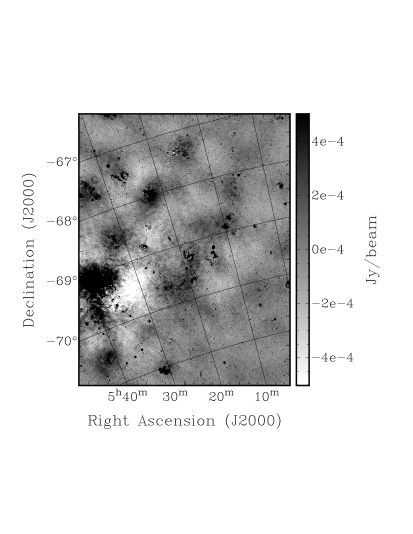
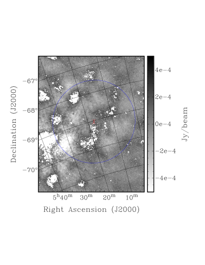
Figure 1: Left panel: Observational map of the LMC at 888 MHz obtained from ASKAP data in Ref. [11]. Right panel: Same as left panel but blanking masked pixels. The red cross indicates the position of the dynamical center and the blue circle encloses the region of interest for this work.

3 LMC description

We compute the radio emission induced by WIMP DM by combining the synchrotron power associated with the LMC magnetic field with the equilibrium distribution ($n_{e}$) of electrons and positrons injected by DM. In order to compute $n_{e}$, we solve a transport equation describing the cooling and spatial diffusion experienced by the electrons and positrons after injection. We describe it in the limit of spherical symmetry and stationarity:

$$-\frac{1}{r^{2}}\frac{\partial}{\partial r}\left[r^{2}D\frac{\partial f}{\partial r}\right]+\frac{1}{p^{2}}\frac{\partial}{\partial p}(\dot{p}p^{2}f)=s(r,p)\;,$$ (3.1)

where $f(r,p)$ is the $e^{+}/e^{-}$ distribution function at the equilibrium, at a given radius $r$ (from the LMC dynamical center) and at a given momentum $p$. The distribution $f$ is related to the number density in the energy interval $(E,E+dE)$ by: $n_{e}(r,E)dE=4\pi\,p^{2}f(r,p)dp$; analogously, for the $e^{+}/e^{-}$ source function, we have $q_{e}(r,E)dE=4\pi\,p^{2}\,s(r,p)dp$. The first term on the left-hand side describes the spatial diffusion, with $D(r,p)$ being the diffusion coefficient. The second term accounts for the energy loss due to radiative processes; $\dot{p}(r,p)=\sum_{i}dp_{i}(r,p)/dt$ is the sum of the rates of momentum loss associated to the radiative process $i$. The DM source $q_{e}$ scales with the number density of WIMP pairs locally in space, i.e., with $\rho^{2}/(2\,M_{\chi}^{2})$, where $\rho(r)$ is the halo mass density profile, and $M_{\chi}$ is the mass of the DM particle. We neglect substructure contributions and assume the DM spatial distribution to be spherically symmetric and static. The source term associated to the production of $e^{+}/e^{-}$ is given by:

$$q^{a}_{e}(E,r)=\langle\sigma_{a}v\rangle\,\frac{\rho(r)^{2}}{2\,M_{\chi}^{2}}\times\frac{dN_{e}^{a}}{dE}(E)\;,$$ (3.2)

where $\langle\sigma_{a}v\rangle$ is the velocity-averaged annihilation rate, and $dN_{e}^{a}/dE$ is the number of electrons/positrons emitted per annihilation in the energy interval $(E,E+dE)$ for a given annihilation channel.

We solve Eq. (3.1) numerically using finite-differencing Crank-Nicolson scheme, for details see Ref. [13]. Boundary conditions are set to be Neumann’s one at the centre and Dirichlet’s one at the farthest boundary, the latter chosen to be ten times the radius of our region of interest (RoI). A recent semi-analytical treatment of Eq. (3.1) can be found in Ref. [15].

The properties we want to constrain are the DM mass and annihilation rate, while the ingredients we need to model are the DM spatial profile, the magnetic field, the spatial diffusion coefficient, the CMB and LMC interstellar radiation fields (ISRF, for inverse Compton losses) and the gas density (for bremsstrahlung losses), that we describe in detail in the following sections. Since our goal is to derive conservative bounds on the WIMP signal, we will model the above quantities taking lower limits for the DM profile and magnetic field, while upper limits for diffusion coefficient and ISRF and gas densities.

To limit uncertainties in the model description, our RoI for the analysis will be defined by a relatively small region around the LMC center, corresponding to 1.3 kpc in radius ($1.5^{\circ}$ in angular units). The loss in terms of J-factor, if compared to considering the full LMC halo, is limited, around a factor of two, depending on the profile. As we will describe in the following, in such RoI we have a more robust determination of the various ingredients entering the computation, such as the magnetic field, the gas and ISRF distributions, and the DM profile. Moreover, we exclude the bulk of the contamination from the 30 Doradus region (south-west in Fig. 1).

3.1 Dark matter profile

To model the radio emission of the LMC due to annihilating DM, the spatial particle distribution $\rho(r)$ is a key ingredient, see Eq. (3.2). Previous work has explored different functional forms for the DM density profile in the LMC [16, 5, 8, 17, 18, 19, 20] and analysed H i rotational [21] and carbon star data [22] to constrain the parameters of $\rho(r)$. In this work we are interested in the inner region, so we make use of the H i data [21] that provide the most accurate rotation velocities at small distances from the LMC dynamical center. We explore four different profiles and fit $\rho(r)$ up to a radius of $\sim 2.7$ kpc from the center, which corresponds to about twice our RoI. In particular, we consider two different “cuspy” DM profiles from the NFW model (Navarro-Frenk-White) [23] and Hernquist [24]:

$$\rho_{\rm{NFW}}(r)=\frac{\rho_{s}}{\left(\frac{r}{r_{S}}\right)\left(1+\frac{r}{r_{s}}\right)^{2}}\;\;\;,\;\;\;\rho_{\rm{Her}}(r)=\frac{\rho_{s}}{\left(\frac{r}{r_{s}}\right)\left(1+\frac{r}{r_{s}}\right)^{3}}\;,$$ (3.3)

and two “cored” profiles, the isothermal sphere [25] and the Burkert profile [26]:

$$\rho_{\rm{Iso}}(r)=\frac{\rho_{s}}{1+\left(\frac{r}{r_{s}}\right)^{2}}\;\;\;,\;\;\;\rho_{\rm{Bur}}(r)=\frac{\rho_{s}}{\left(1+\frac{r}{r_{s}}\right)\left(1+\left(\frac{r}{r_{s}}\right)^{2}\right)}\;.$$ (3.4)

The main reason for considering different shapes is related to our poor knowledge about DM physics at small scales, including the possible role of baryons in affecting the DM spatial profile. The range of possibilities encompassed by the above functional forms should bracket the uncertainty.

The free parameters of the different profiles are the scale radius $r_{s}$ and the normalization $\rho_{s}$. We fit these values for each profile using the H i  rotation velocity data and the fact that the velocity $v(r)$ measured up to a radius $r$ is given by the expression

$$v(r)=\sqrt{\frac{GM_{\rm{tot}}(r)}{r}},$$ (3.5)

where $M_{\rm{tot}}(r)$ is the total mass contained within a radius $r$, given by DM plus contributions from the stellar and gas components. We model the stellar potential $\phi_{\star}(R,z)$ using a Plummer-Kuzmin disk [27] as a function of the disk radial distance $R$ and vertical height $z$ in cylindrical coordinates:

$$\phi_{\star}(R,z)=GM_{\star}\left[R^{2}+\left(a_{\star}+\sqrt{z^{2}+b_{\star}^{2}}\right)^{2}\right]^{-1/2},$$ (3.6)

where $a_{\star}$ and $b_{\star}$ are the radial scale length and vertical scale height, respectively, for which we take $a_{\star}=1.7$ kpc and $b_{\star}=0.34$ kpc [28, 29]. The stellar mass $M_{\star}$ is left as a free parameter in the fit. The contribution to the mass density $\rho_{g}(R,z)$ from the gas follows the expression given in Ref. [29] (with radial scale length $a_{g}=a_{\star}$ and vertical scale height $b_{g}=b_{\star}$):

$$\rho_{g}(r,z)=\frac{M_{g}}{2\pi a_{g}^{2}b_{g}}\,0.5^{2}\,{\rm sech}\left(\frac{R}{a_{g}}\right){\rm sech}\left(\frac{|z|}{b_{g}}\right).$$ (3.7)

Once we have the total mass contribution from the different components to the rotation velocity at some radius $r$, we proceed to fit the parameters $r_{s}$, $\rho_{s}$ and $M_{\star}$ using a least squares method through the python package scipy.optimize. The best-fit parameters for the different DM density profiles are shown on Table 1. For simplicity, and since the gas component provides a subdominant contribution to the matter density, we set $M_{g}=5\times 10^{8}\,M_{\odot}$. Nevertheless, we checked that the results for $r_{s}$ and $\rho_{s}$ reported on Table 1 are unchanged if $M_{g}$ is left as a free parameter in the fit.

Previous work has suggested that the LMC virial mass is around $2\times 10^{11}M_{\odot}$, but estimates can have significant uncertainties [3, 20, 18]. On the other hand, the virial mass is mostly related to the DM profile at larger radii than the one relevant for our analysis (the enclosed mass in our RoI is $\lesssim 2\times 10^{10}M_{\odot}$), making these uncertainties of little relevance for our results. We adopt different values for the LMC virial mass, corresponding to Table 2 from Ref. [20], in order to normalize the profiles. We find that the rotation velocity within $\sim 5$ kpc from the center of the LMC, as well as the profile parameters determined by our fit, do not change considerably with different choices for the mass normalization. Therefore we adopt a (low) virial mass of $10^{11}M_{\odot}$.

Profile	$r_{s}$ [kpc]	$\rho_{s}$ $[M_{\odot}/\rm{kcp}^{3}]$	$M_{\star}$ $[M_{\odot}]$
NFW	9.8	$5.1\times 10^{6}$	$1.0\times 10^{9}$
Isothermal	1.1	$5.7\times 10^{7}$	$1.9\times 10^{9}$
Burket	4.7	$3.1\times 10^{7}$	$1.9\times 10^{9}$
Hernquist	21.8	$2.1\times 10^{6}$	$1.0\times 10^{9}$

Table 1: Parameters for the LMC DM density profiles and stellar mass derived from the rotation curve fit, see Section 3.1.

The results are shown in Figure 2, where we report the contributions to the rotation velocity from DM (dashed lines), stellar and gas components (red dots and green crosses respectively). The orange points represent the H i  rotation data from Ref. [21] and the solid lines show the contribution from the sum of all components.

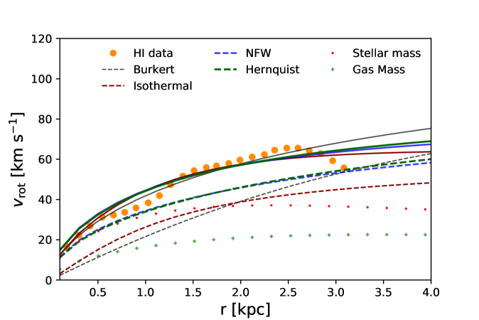
Figure 2: LMC rotation curve. The H i  rotation data points are shown as orange dots [21]. Dashed lines show the contribution from the enclosed DM mass for the different profiles assumed (see Section 3.1). Red dots and green crosses denote the stellar and gas contributions respectively. Solid lines correspond to the contribution of all the enclosed mass within a radius $r$ (DM+stellar+gas).

3.2 Magnetic field and diffusion coefficient

The strength of the large-scale coherent component of the LMC magnetic field is found to be $1\,\mu$G, as determined via Faraday rotation measure of polarized background sources [6], and with diffuse polarized data [30] (see also [31]). The turbulent component is expected to be larger than the regular one, by a factor $>3$, as generically found in galaxies (see, e.g., Ref. [32]), and confirmed by the scatter observed in the LMC rotation measures [30]. In Ref. [6], the total LMC magnetic field strength on large scales has been estimated to be $B=4.3\,\mu$G, and we take this as our reference value. We focus on a relatively small and central region of LMC, where rotation measures do not show significant dependence on the radial distance, so we can assume a uniform strength, in agreement with the model in Ref. [30]. Amplifications on small scales [6] are disregarded. A recent analysis based on the equipartition assumption and on observations of the LMC synchrotron emission at 166 MHz [33] suggests a higher value, $B=7.7\pm 1.1\,\mu$G. Since the magnetic field is (together with the DM properties) the most crucial ingredient of our analysis, we show how our results change for a range of total strength $B=2-8\,\mu$G. This range is in agreement with estimates stemming from the cosmic-ray density derived from $\gamma$-ray data and again applying the equipartition assumption [30].

Data on supernovae remnants [34] and on large-scale diffuse emission [35] indicate that the transport of cosmic-rays in the LMC proceeds in a similar way as in other nearby galaxies, and can be explained as diffusive propagation in a turbulent regime. In this scenario, the diffusion coefficient can be estimated as [35]:

$$D\simeq 3\,\times 10^{27}\,\left(\frac{d_{L}}{{\rm kpc}}\right)^{2}\,\left(\frac{10^{15}\,{\rm s}}{\tau}\right){\rm\frac{cm^{2}}{s}}\;,$$ (3.8)

where $d_{L}$ is the diffusion length and $\tau$ is the cooling time. Radio observations suggest $d_{L}\simeq 1-2$ kpc in the vertical direction (larger along the disk), consistent with findings in other galaxies where the confinement region is a few times the disk height. The discussion on radiative losses below leads to $\tau\simeq 10^{15}$ s, in agreement with the limit of $\tau>10^{14}$ s estimated in Ref. [34].

Thus observations point towards a value somewhat lower than in the Galaxy. For clarity, and in the spirit of making conservative assumptions, we assume the same strength and energy dependence of the diffusion coefficient as at large scales in the Galaxy, taking the latest determination from Ref. [36] (BIG model, which provides $2\,\times 10^{28}\,{\rm cm^{2}/s}$ at 4 GeV). Recall that the larger the diffusion coefficient the smaller the DM signal, since diffusion can remove electrons and positrons from the RoI before they emit synchrotron radiation at the frequency of interest.

3.3 Gas and interstellar radiation fields

We determine the central value of the gas density from Eq. (3.7) and taking $M_{g}=5\times 10^{8}\,M_{\odot}$, which is the neutral hydrogen mass observed by Ref. [21]. Then we assume a flat spatial profile, normalized to the maximal value, i.e., the central value, which leads to the gas number density $n_{g}=\rho(0,0)/m_{H}=0.8\,{\rm cm^{-3}}$ (where $m_{H}=0.938$ GeV is the hydrogen atom mass). This is clearly a conservative approach. Moreover it simplifies the computation by avoiding uncertainties related to the radial and vertical scale lengths of the gas distribution and allowing us to keep assuming spherical symmetry. We checked this description by deriving the gas density from the hydrogen column density in Fig.4 of Ref. [37] divided by a disk thickness of 350 pc [37]. The spatial profile does not show significant variations in our RoI (justifying a flat model) and the average value for the column density is $6\times 10^{20}\,{\rm cm}^{-2}$, which translates into $n_{g}\simeq 0.5\,{\rm cm^{-3}}$, confirming the above assumption for $n_{g}$ as an upper limit.

We assume the gas to be composed solely of neutral atomic hydrogen, since molecular hydrogen and ionised gas are subdominant components [38, 39, 6], negligible in this analysis.

The ISRF spectrum is taken to have the same shape as that of the Milky-Way [40]. Observationally, this is found to be a good approximation [41]. Moreover, even though we implement a full computation, the Klein-Nishina corrections are subdominant (the energy of the emitting electrons is $\lesssim 10$ GeV), so the exact ISRF spectral shape is not critical, and the size of the inverse Compton losses is essentially set by the integral over energy.

The normalization is chosen such that the integral of the spectrum provides $U_{\rm{ISRF}}=1\,{\rm eV/cm^{3}}$, consistent with the parameter $X_{\rm{ISRF}}$ found in Ref. [41]. We note that a somewhat lower density can be derived from the LMC SED of Ref. [42], see Ref. [43] who found $U_{\rm{ISRF}}=0.57\,{\rm eV/cm^{3}}$, and using the estimate of Ref. [35] where $U_{\rm{ISRF}}\simeq 0.3\,{\rm eV/cm^{3}}$. Again, our choice is in the spirit of adopting a realistic upper limit.

As for the gas density, we conservatively take a spatially flat profile.

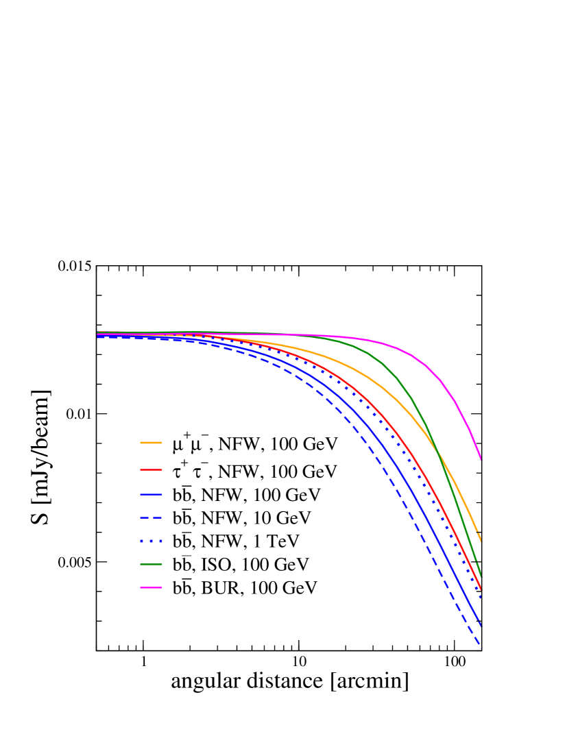
Figure 3: Left panel: Model of LMC diffuse emission: disk+DM. Right panel: WIMP emission profile as a function of the angular distance from the LMC center, for different WIMP masses, annihilation channels, and spatial profiles (with the magnetic field strength taken to be $B=4.3\,\mu$G).

4 Results

We assume the likelihood associated with the LMC diffuse emission to be described by a Gaussian:

$$\mathcal{L}=e^{-\chi^{2}/2}\;\;\;{\rm with}\;\;\;\chi^{2}=\frac{1}{N_{pix}^{FWHM}}\sum_{i=1}^{N_{pix}}\left(\frac{S_{th}^{i}-S_{obs}^{i}}{\sigma_{rms}^{i}}\right)^{2}\;,$$ (4.1)

where $S_{th}^{i}$ is the theoretical estimate for the flux density in the pixel $i$, $S_{obs}^{i}$ is the observed flux density and $\sigma_{rms}^{i}$ is the r.m.s. error, both described in Sec. 2. $N_{pix}$ is the total number of pixels in the RoI (excluding masked pixels) and $N_{pix}^{FWHM}$ is the number of pixels within the FWHM of the synthesized beam. We only include the DM signal coming from inside a sphere of radius of 1.3 kpc around the LMC center (thus disregarding other line-of-sight DM contributions inside the angular region of $90^{\prime}$). The theoretical estimate is provided by the WIMP emission, computed from the solution of Eq. (3.1) and following Sec. 4.1 in Ref. [13], plus a disk component and a spatially flat term.

The disk is described through a Gaussian $S_{disc}^{i}=S_{0}\,\exp{[-\theta_{d,i}^{2}/(2\,\theta_{0}^{2})]}$, where $\theta_{d,i}$ is the angular distance of the pixel $i$ from the axis of the disk, and $S_{0}$ and $\theta_{0}$ are free parameters. The position angle of the LMC disk has been found to be between $122.5^{\circ}$ and $170.5^{\circ}$, depending on the tracer (see Ref. [44] and references therein). In our analysis we assume a value determined by fitting the map without including the DM component. We find $138^{\circ}$, similar to that found recently using Gaia DR2 data [45].

In Fig. 3 (left), we show the shape of the model given by disk plus DM. We use arbitrary normalization and fix the FWHM of the Gaussian describing the disk to $0.45^{\circ}$ (which is the best-fit value found in the fit).

On top of the disk component we add a spatially flat term $S_{flat}$. This is included in the fit to account for possible offsets or a large-scale foreground component. The parameters $S_{flat}$, $S_{0}$ and $\theta_{0}$ are treated as nuisance parameters.

In Fig. 3 (right), we show the WIMP emission as a function of the angular distance from the center, for different masses, annihilation channels and DM density profiles. Note that the size of the DM source is below 2 degrees. The NFW profile is the most concentrated case (together with the Hernquist profile, which is not shown since it is nearly identical to the NFW at small distances). The Burkert and isothermal profiles provide more extended distributions. Note that high masses and leptonic channels imply a less concentrated profile than low masses and hadronic channels. This can be understood by noting that at the frequency of the observations (888 MHz) and for a magnetic field of $4.3\,\mu$G, the synchrotron emission is mostly provided by $e^{+}/e^{-}$ with energy around a few GeV. High energy electrons take time to cool down to few GeV and thus can travel long distances, flattening the central overdensity. Recall that leptonic channels provide harder $e^{+}e^{-}$ spectra than in the $b\bar{b}$ case.

Bounds on the parameter $\langle\sigma_{a}v\rangle$ are computed at any given mass $M_{\chi}$ through a profile likelihood technique [46], namely “profiling out” the nuisance parameters $\vec{\Pi}=(S_{flat},S_{0},\theta_{0})$. We assume that $\lambda_{c}(\langle\sigma_{a}v\rangle)=-2\ln[\mathcal{L}(\langle\sigma_{a}v\rangle,\vec{\Pi}^{b.f.})/\mathcal{L}(\langle\sigma_{a}v\rangle^{b.f.},\vec{\Pi}^{b.f.})]$ follows a $\chi^{2}$-distribution with one d.o.f. and with one-sided probability given by $P=\int^{\infty}_{\sqrt{\lambda_{c}}}d\chi\,e^{-\chi^{2}/2}/\sqrt{2\,\pi}$, where $\langle\sigma_{a}v\rangle^{b.f.}$ denotes the best-fit value for the annihilation rate at that specific WIMP mass. Therefore, the 95% C.L. upper limit on $\langle\sigma_{a}v\rangle$ at mass $M_{\chi}$ is obtained by increasing the signal from its best-fit value until $\lambda_{c}=2.71$, keeping $\vec{\Pi}$ fixed to its best-fit value.

The possible presence of a DM signal is investigated by evaluating the difference $\Delta\chi^{2}=\chi^{2}(\vec{\Pi}^{b.f.},\langle\sigma_{a}v\rangle=0)-\chi^{2}(\vec{\Pi}^{b.f.},\langle\sigma_{a}v\rangle_{b.f.})$, We always find $\Delta\chi^{2}<1$, and thus no evidence for a diffuse component associated with WIMP-induced emission.

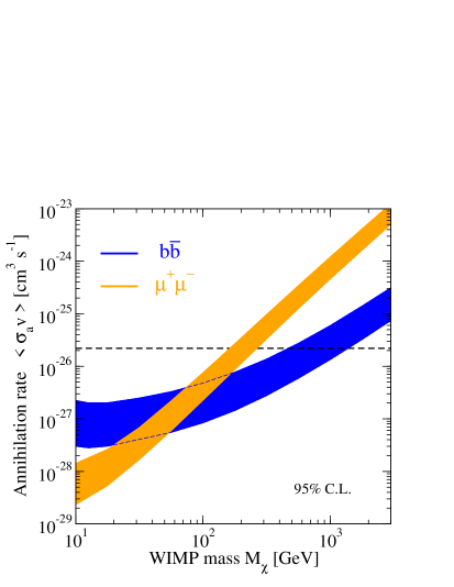
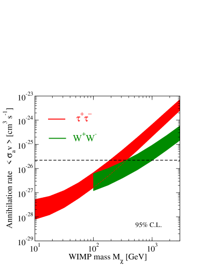
Figure 4: 95% C.L. upper limits on $\langle\sigma_{a}v\rangle$ as a function of $M_{\chi}$ for the annihilation channels $b\bar{b}$ (blue), $\mu^{+}\mu^{-}$ (orange), $\tau^{+}\tau^{-}$ (red), and $W^{+}W^{-}$ (green), with the magnetic field strength taken to be $B=4.3\,\mu$G.

Results are shown in Fig. 4, reporting the upper limits on $\langle\sigma_{a}v\rangle$. The boundaries of the uncertainty band are determined by taking the weakest/strongest bound among those obtained using the four different DM profiles described in Section 3.1. More concentrated profiles provide more stringent constraints. The NFW and Hernquist cases set the lower boundary of the band, while Burkert at low masses and Isothermal at high masses set the upper boundary. The dashed black line is the so-called thermal cross section, namely the self-annihilation cross section needed in the early Universe in order to provide the DM mass density observed today [47]. A common way to see Fig. 4 is to consider “canonical” WIMPs excluded for masses where the bound is below the thermal value.

The trend of the bound is similar for the $b\bar{b}$ (blue) and $W^{+}W^{-}$ (green) channels, on one hand, and for $\tau^{+}\tau^{-}$ (red) and $\mu^{+}\mu^{-}$ (orange) channels, on the other. The reason is related to the injection spectrum of $e^{+}e^{-}$. Let us first remind that the key quantity is the density of $e^{+}/e^{-}$ induced by the specific DM model at energies of a few GeV. The injection spectrum of $e^{+}e^{-}$ is harder in the leptonic cases, where WIMPs with mass of tens of GeV have therefore a significant injection of $e^{+}e^{-}$ with energy around the peak of the synchrotron power. This makes the bounds in the $\tau^{+}\tau^{-}$ and $\mu^{+}\mu^{-}$ cases very tight at low masses. Clearly, the picture is the opposite at high masses where the injection energy is “too high” and the $e^{+}e^{-}$ undergo energy losses and diffusion before emitting synchrotron radiation. In the cases of $b\bar{b}$ and $W^{+}W^{-}$, the peak in the injection of $e^{+}e^{-}$ occurs at around $M_{\chi}/20$. Therefore, they are more efficiently constrained in the range of masses around hundreds of GeV (so that, again, the production of $e^{+}/e^{-}$ is peaked around a few GeV).

Since we consider non-relativistic DM, the WIMP mass has to be larger than the mass of the annihilation products, and this is the reason of the cut in the $W^{+}W^{-}$ bound.

The overall increase of the constraints with the WIMP mass, occurring for all the channels, can be understood from Eq. (3.2).

The bottom line of Fig. 4 is that the thermal cross-section is excluded for masses below (480, 358, 192, 164) GeV for the ($b\bar{b}$, $W^{+}W^{-}$, $\tau^{+}\tau^{-}$, $\mu^{+}\mu^{-}$) annihilation channel.

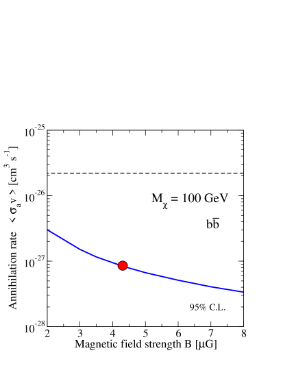
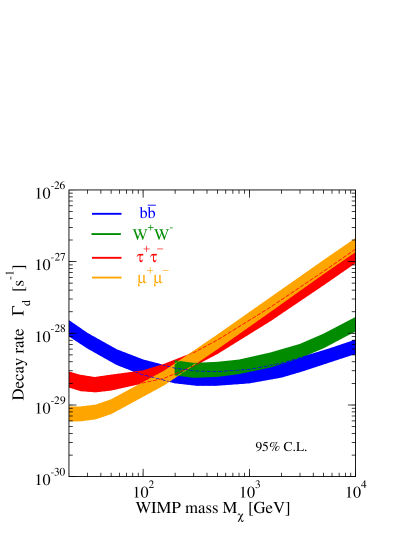
Figure 5: Left panel: Impact of the magnetic field strength on the bound on $\langle\sigma_{a}v\rangle$, in an example taking $M_{\chi}=100$ GeV, annihilation into $b\bar{b}$, and NFW DM profile. The red dot shows the reference value adopted in this work. Right panel: 95% C.L. upper limits on the decay rate $\Gamma$ as a function of $M_{\chi}$ for the decay channels $b\bar{b}$ (blue), $\mu^{+}\mu^{-}$ (orange), $\tau^{+}\tau^{-}$ (red), and $W^{+}W^{-}$ (green), with the magnetic field strength taken to be $B=4.3\,\mu$G.

In Fig. 5 (left), we show how the magnetic field strength affects the bound on $\langle\sigma_{a}v\rangle$. We consider an example with $M_{\chi}=100$ GeV, annihilation into $b\bar{b}$, and NFW DM profile. The bound approximately scales with the inverse of the square of the magnetic field for small strengths, and flattens as the strength increases. As already stated, in Fig. 4 we adopted $B=4.3\,\mu$G.

Throughout the paper, we have been assuming annihilating DM. In the right panel of Fig. 5 we show the bounds that can be obtained for decaying DM. The only difference from the above analysis consists in the replacement of Eq. (3.2) with

$$q^{d}_{e}(E,r)=\Gamma_{d}\,\frac{\rho(r)}{M_{\chi}}\times\frac{dN_{e}^{d}}{dE}(E)\;,$$ (4.2)

where $\Gamma_{d}$ is the decay rate, and $dN_{e}^{d}/dE$ is the number of electrons/positrons emitted per decay in the energy interval $(E,E+dE)$.

The different behaviour of the four decaying channels can be understood in a very similar way to that already discussed above for the annihilating case. Note that the uncertainty band of the curves in Fig. 5 is smaller than in the annihilating cases of Fig. 4. This is because the source function of annihilating DM depends on $\rho^{2}$, while the decaying scenario scales linearly with $\rho$, and thus uncertainties in the DM spatial profile affect the former more than the latter.

5 Comparison with previous work

We focus the comparison with previous analyses on work investigating the LMC and dwarf galaxies, i.e., satellites of the Milky Way, since they share a similar analysis as that conducted here. We do not attempt to make comparisons with completely different targets (e.g., the Galactic Center) or channels (e.g., antiprotons). For other analyses using radio data to constrain WIMP annihilations in extragalactic objects, see, e.g., Refs. [48, 49, 50] (M31), [51, 52] (M33), [53, 54] (clusters), [55, 56] (cosmological emission).

5.1 Comparison with radio analyses

An analysis similar to the one presented here was conducted in Ref. [8]. They employed ATCA+Parkes data and obtained the black curve in Fig. 6 (left). The great improvement in the constraining power of our analysis is not due to the model, for which we adopted a more conservative description than Ref. [8], but to the different statistical approach and to the more limited residuals and higher rms sensitivity in the ASKAP image compared to the ATCA+Parkes image. Concerning the statistical analysis, Ref. [8] derived the bound from individual lines of sight, while we developed a morphological analysis. The latter allows us to ascribe part of the LMC emission to a disk component and combines $\sim 10^{4}$ lines of sight. This is important since the constraining power scales roughly as the square root of this number.

There have been a few attempts to detect WIMP-induced radio signals in dwarf spheroidal galaxies of the Local Group. We expect the signal from LMC to be stronger than from dSphs since the magnetic field strength is higher (it is actually unknown in dSph, but typically assumed to be around 1 $\mu$G [13]), the J-factor is higher than (or at the level of) that in the most promising dSphs, and the LMC is bigger (which means diffusion effects are less relevant in depleting the signal than in dSphs). In Fig. 6, we include bounds derived from the observations of different samples of dSphs with the ATCA from Ref. [57] (taking their model with $B=1\,\mu{\rm G}\;,\;D_{0}=3\,\times 10^{28}\,{\rm cm^{2}/s}$, red solid line) and Ref. [58] (AVE model, red dashed line), GMRT [59] ($B=2\,\mu{\rm G}\;,\;D_{0}=3\,\times 10^{28}\,{\rm cm^{2}/s}$, violet line), LOFAR [60] ($B=1\,\mu{\rm G}\;,\;D_{0}=10^{27}\,{\rm cm^{2}/s}$, orange line), MWA+GMRT [61] ($B=2\,\mu{\rm G}\;,\;D_{0}=3\,\times 10^{28}\,{\rm cm^{2}/s}$, magenta line). Other relevant campaigns have been conducted with the GBT [62, 63, 64] and MWA [65]. Their bounds are not in a suitable form to be shown in Fig. 6, but correspond to about $\langle\sigma_{a}v\rangle\lesssim 10^{-24}{\rm cm^{3}/s}$ for $M_{\chi}=100$ GeV and the $b\bar{b}$ channel.

5.2 Comparison with $\gamma$-ray analyses

In Fig. 6 (right), we compare the results of this work with the bounds obtained by the Fermi-LAT Collaboration from the analysis of the LMC [16] and dSphs [66]. For completeness we also show the expected LMC bounds from the Cherenkov Telescope Array [67], since they can be more constraining than those from Fermi-LAT at high WIMP masses.

One can immediately see that the LMC radio constraints are much stronger than $\gamma$-ray ones. This should not come as a surprise. Indeed, generically, in WIMP models, the luminosity associated with the induced $\gamma$-rays is comparable to or smaller than that of the injected electrons and positrons. For hadronic channels, the $\gamma$-ray emission mainly proceeds through the production and decay of neutral pions, while electron/positron injection is related to charged pions, and so the two mechanisms are tightly related. For leptonic channels, GeV electrons and positrons have a larger yield than the final state radiation of $\gamma$-ray photons. Therefore, if the cooling time/diffusion length is small enough, so that the energy of the electron/positron is radiated within the source, and the synchrotron loss is the dominant (or, at least, among the most relevant) radiation mechanism in the astrophysical object under investigation, the luminosity produced as synchrotron radiation is comparable to or higher than that from $\gamma$-rays [2]. Since radio telescopes are much more sensitive than $\gamma$-ray telescopes for all sources having related mechanisms of emission in the two bands (see, e.g., the level of detail in the ASKAP LMC image compared to the $\gamma$-ray image of the LMC [68]), radio bounds on WIMPs are significantly stronger, when above conditions are satisfied, and in particular for objects with low astrophysical diffuse radio background, such as the LMC.

The picture is different for dSphs, since there the diffusion length is typically larger than the galaxy itself and the magnetic field is thought to be rather small (and so too the synchrotron radiation), which implies a less favourable ratio between radio and $\gamma$ bounds, even though still comparable (see red solid line in the left panel versus orange line in the right panel).

Fig. 6 shows that the bound derived in this work is the most stringent bound on WIMPs coming from indirect searches in extragalactic objects.

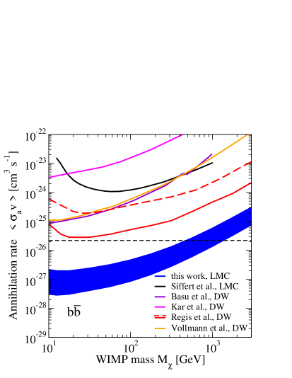
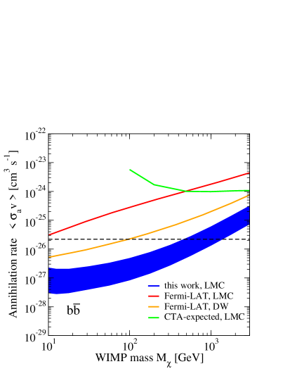
Figure 6: Left panel: Comparison with other radio searches, see text for details. “DW” labels analyses of dwarf spheroidal galaxies. Right panel: Comparison with $\gamma$-ray Fermi-LAT searches on dwarf spheroidals [66] (orange) and on the LMC [16], and with the expected sensitivity of CTA for LMC [67].

6 Conclusions

We analysed the ASKAP radio image at 888 MHz of the LMC, in order to search for synchrotron emission induced by WIMP DM annihilations.

The large J-factor of the LMC implies it is one of the best targets for DM indirect searches. The presence of a magnetic field with strength $>1\,\mu$G makes radio searches in the LMC particularly suited for this purpose.

We detect no evidence for emission arising from WIMP annihilations and derive stringent bounds. Annihilations into leptonic channels provide the most constraining bounds at low masses with the thermal cross-section excluded for masses below 192 GeV ($\tau^{+}\tau^{-}$) and 164 GeV ($\mu^{+}\mu^{-}$). Annihilations into quarks and gauge bosons are the most constraining cases at intermediate and high masses with the thermal cross-section excluded below 480 GeV ($b\bar{b}$) and 358 GeV ($W^{+}W^{-}$).

The comparison with the state-of-the-art in Fig. 6 shows that the bounds on WIMPs derived in this work are extremely competitive.

We adopted a simple and conservative approach, limiting the analysis to a relatively small region, where simplified assumptions and well-motivated data-driven descriptions can be taken for the astrophysical ingredients entering the model prediction. For the two most relevant quantities, the DM spatial profile and the magnetic field, we defined reference models according to observations [21, 6]. For the other components (which are important for the computation, but to a somewhat lesser extent), such as the spatial diffusion coefficient, the interstellar radiation fields, and the gas density, we consider their upper or lower limits (all in the direction of minimising the DM signal).

Our results imply there is little hope to detect a signal from low mass thermal WIMPs in laboratories (i.e., in direct and collider searches), whilst very massive thermal WIMPs remain a viable DM candidate. They can be probed by different techniques, including observations from future radio telescopes, such as the SKA, in particular going to higher frequencies. On a shorter timescale, the addition of short spacing data coming from forthcoming observations with the Parkes telescope will provide a complete picture of the LMC at different scales. With such image at hand, a more refined 3D modeling of the synchrotron emission from the entire LMC can be attempted, with the possibility of further tightening the bounds derived in this analysis.

Appendix A Consistency checks

In this Appendix, we describe a few consistency checks we performed.

First, a key and not obvious (for an interferometric image) point is the actual sensitivity of the image to large scale diffuse emissions. In order to understand how the sensitivity scales as a function of the size of the source, we taper the visibilities by different angular scales, generate an image with robust weighting, and then measure the standard deviation in the image. For technical reasons and since here we are mainly interested in understanding the trend but not the absolute value, we performed the analysis on Stokes V and considering one of the LMC pointings (all pointings were taken at similar directions and times). The rms sensitivity normalized to one at 2 arcmin is plotted in Fig. 7 (red line) as a function of the tapering size.

In the same figure, the blue line reports the total flux of a source which is excluded at 95% C.L. by the analysis described in the main text, as a function of the angular scale of the source. Again values are normalized to one for a source with FWHM$=2$ arcmin. One can quickly check that, in the case of uniform rms, no masking and no confusion, Eq. (4.1) would imply a linear scaling. The blue curve is derived by considering Gaussian sources of different widths (essentially replacing the DM component with a Gaussian emission and then repeating all the steps described in Sects. 3 and 4). The actual behaviour is close to linear scaling.

The bottom-line of Fig. 7 is that the “theoretical” degradation of the sensitivity as the angular scale of the sources increases, as assumed by the analysis described in the paper, is higher if compared to the results obtained through the tapering test. This ensures our bounds are conservative.

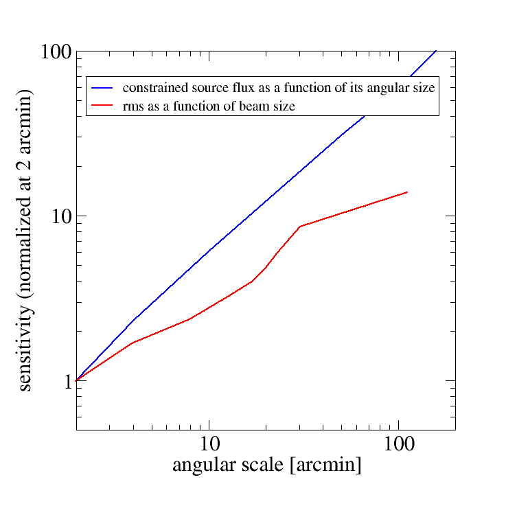
Figure 7: The red line shows the rms sensitivity of the LMC image as a function of the tapering size. The blue curve shows the total flux excluded by the analysis described in the main text as a function of the size of the source. Both curves are normalized to one at two arcmin.

To test against possible systematics associated to the selected region of the image, we re-do the same analysis outlined in the main text, but now centering the DM distribution on different positions across the map. Since we are dealing with a non-detection, they should all provide similar bounds, because the RMS sensitivity is approximately uniform across the map. We compare five different positions, as listed in Fig. 8 (left). Concerning the DM model we take the same description as in Section 3, but centered in the new positions. This is clearly not realistic, but functional to our test. We find that positions that are far from the LMC disk (i.e., $C$ and $D$ in Fig. 8) provide slightly more constraining bounds, with the component $S_{disc}$ compatible with zero. Positions located on the LMC disk (i.e., $B$ and $E$ in Fig. 8) lead to bounds similar to the ones described in the main text (case $A$), with the fit requiring a disk component different from zero. Fig. 8 (left) reports the bound in the case of the NFW profile and annihilation into $b\bar{b}$.

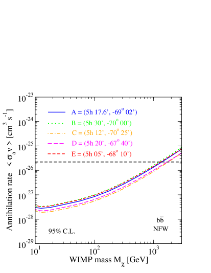
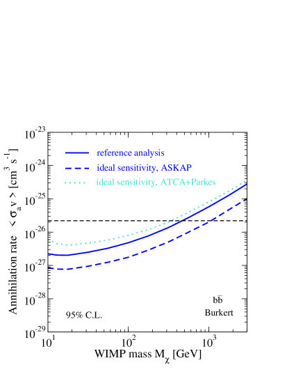
Figure 8: Left panel: Comparison of the bounds obtained by centering the DM distribution on different positions across the map (labeled as A, B, C, D and E to easy their reference in the text). Right panel: Comparison of the bounds obtained in the reference analysis of this work (solid) with the bounds one would obtain considering the maximal ideal sensitivity of the EMU image (dashed) and analysing the ATCA+Parkes image of Ref. [69] (dotted).

In Fig. 8 (right) we compare our results with the maximal sensitivity that can be achieved with the image we have at hand. The latter is derived by keeping the original resolution (FWHM=13”) and evaluating $\chi^{2}=\sum_{i=1}^{N_{pix}}\left(\frac{S_{DM}^{i}}{\sigma_{rms}^{i}}\right)^{2}/N_{pix}^{FWHM}$, which can be seen as setting to zero all pixels in the map (after RMS determination). We show the result for the Burkert profile since it is the most extended case, so where the number of pixels relevant for the $\chi^{2}$ determination is largest, which implies the sensitivity difference is largest. As expected the bound derived with such ideal sensitivity is more constraining than for our reference analysis, but by a rather limited factor (between 2 and 3).

In the same Figure, we derive WIMP bounds from the LMC map at 1.4 GHz presented in Ref. [69]. Such map contains all scales above $40^{\prime\prime}$ being a combination of ATCA and (single-dish) Parkes data, contrary to the ASKAP image having only interferometric data. This means that the very large-scale emission would need a more careful treatment than the simple model introduced in Section 3. For this reason, we perform the comparison in the “ideal-sensitivity” case. The analysis of ATCA+Parkes data is performed in the same way as for the ASKAP map. From the ratio of the RMS sensitivity of the two maps (300 versus 58 $\mu$Jy/beam), and considering the different frequency (1.4 versus 0.888 GHz) and beam (40” versus 13”), we expect the ATCA+Parkes bound to be a factor around 5 weaker than the ASKAP one. Results are along the line of expectations, see dotted versus dashed lines, providing a consistency check.

References

- [1] J. Silk et al. Particle Dark Matter: Observations, Models and Searches. Cambridge Univ. Press, Cambridge, 2010.
- [2] Marco Regis and Piero Ullio. Multi-wavelength signals of dark matter annihilations at the Galactic center. Phys. Rev. D, 78:043505, 2008, 0802.0234.
- [3] Nitya Kallivayalil, Roeland P. van der Marel, Gurtina Besla, Jay Anderson, and Charles Alcock. THIRD-EPOCH MAGELLANIC CLOUD PROPER MOTIONS. i.HUBBLE SPACE TELESCOPE/WFC3 DATA AND ORBIT IMPLICATIONS. The Astrophysical Journal, 764(2):161, feb 2013.
- [4] Gisella Clementini, Raffaele Gratton, Angela Bragaglia, Eugenio Carretta, Luca Di Fabrizio, and Marcella Maio. Distance to the large magellanic cloud: The RR lyrae stars. The Astronomical Journal, 125(3):1309–1329, mar 2003.
- [5] Matthew R. Buckley, Eric Charles, Jennifer M. Gaskins, Alyson M. Brooks, Alex Drlica-Wagner, Pierrick Martin, and Geng Zhao. Search for Gamma-ray Emission from Dark Matter Annihilation in the Large Magellanic Cloud with the Fermi Large Area Telescope. Phys. Rev. D, 91(10):102001, 2015, 1502.01020.
- [6] B. M. Gaensler, M. Haverkorn, L. Staveley-Smith, J. M. Dickey, N. M. McClure-Griffiths, J. R. Dickel, and M. Wolleben. The Magnetic Field of the Large Magellanic Cloud Revealed Through Faraday Rotation. Science, 307(5715):1610–1612, March 2005, astro-ph/0503226.
- [7] Argyro Tasitsiomi, Jennifer Gaskins, and Angela V. Olinto. Gamma-ray and synchrotron emission from neutralino annihilation in the Large Magellanic Cloud. Astroparticle Physics, 21(6):637–650, September 2004, astro-ph/0307375.
- [8] Beatriz B. Siffert, Angelo Limone, Enrico Borriello, Giuseppe Longo, and Gennaro Miele. Radio emission from dark matter annihilation in the Large Magellanic Cloud. ”Mon. Not. Roy. Astron. Soc.”, 410(4):2463–2471, February 2011, 1006.5325.
- [9] A. W. Hotan, J. D. Bunton, A. P. Chippendale, M. Whiting, J. Tuthill, V. A. Moss, D. McConnell, S. W. Amy, M. T. Huynh, J. R. Allison, C. S. Anderson, K. W. Bannister, E. Bastholm, R. Beresford, D. C. J. Bock, R. Bolton, J. M. Chapman, K. Chow, J. D. Collier, F. R. Cooray, T. J. Cornwell, P. J. Diamond, P. G. Edwards, I. J. Feain, T. M. O. Franzen, D. George, N. Gupta, G. A. Hampson, L. Harvey-Smith, D. B. Hayman, I. Heywood, C. Jacka, C. A. Jackson, S. Jackson, K. Jeganathan, S. Johnston, M. Kesteven, D. Kleiner, B. S. Koribalski, K. Lee-Waddell, E. Lenc, E. S. Lensson, S. Mackay, E. K. Mahony, N. M. McClure-Griffiths, R. McConigley, P. Mirtschin, A. K. Ng, R. P. Norris, S. E. Pearce, C. Phillips, M. A. Pilawa, W. Raja, J. E. Reynolds, P. Roberts, D. N. Roxby, E. M. Sadler, M. Shields, A. E. T. Schinckel, P. Serra, R. D. Shaw, T. Sweetnam, E. R. Troup, A. Tzioumis, M. A. Voronkov, and T. Westmeier. Australian square kilometre array pathfinder: I. system description. Publications of the Astronomical Society of Australia, 38:e009, March 2021, 2102.01870.
- [10] Ray P. Norris, A. M. Hopkins, J. Afonso, S. Brown, J. J. Condon, L. Dunne, I. Feain, R. Hollow, M. Jarvis, M. Johnston-Hollitt, and et al. Emu: Evolutionary map of the universe. Publications of the Astronomical Society of Australia, 28(3):215–248, 2011.
- [11] Clara M. Pennock and et al. The askap-emu early science project: 888 mhz radio continuum survey of the large magellanic cloud. ”Mon. Not. Roy. Astron. Soc., in press”, 2021.
- [12] E. Bertin and S. Arnouts. SExtractor: Software for source extraction. Astron. Astrophys. Suppl. Ser., 117:393–404, June 1996.
- [13] Marco Regis, Laura Richter, Sergio Colafrancesco, Stefano Profumo, W. J. G. de Blok, and M. Massardi. Local Group dSph radio survey with ATCA – II. Non-thermal diffuse emission. Mon. Not. Roy. Astron. Soc., 448(4):3747–3765, 2015, 1407.5482.
- [14] R. J. Sault, P. J. Teuben, and M. C. H. Wright. A Retrospective View of MIRIAD. In R. A. Shaw, H. E. Payne, and J. J. E. Hayes, editors, Astronomical Data Analysis Software and Systems IV, volume 77 of Astronomical Society of the Pacific Conference Series, page 433, 1995.
- [15] Martin Vollmann. Universal profiles for radio searches of dark matter in dwarf galaxies. arXiv e-prints, page arXiv:2011.11947, November 2020, 2011.11947.
- [16] Matthew R. Buckley, Eric Charles, Jennifer M. Gaskins, Alyson M. Brooks, Alex Drlica-Wagner, Pierrick Martin, and Geng Zhao. Search for gamma-ray emission from dark matter annihilation in the large magellanic cloud with the fermi large area telescope. Phys. Rev. D, 91:102001, May 2015.
- [17] R. Caputo, M. R. Buckley, P. Martin, E. Charles, A. M. Brooks, A. Drlica-Wagner, J. Gaskins, and M. Wood. Search for gamma-ray emission from dark matter annihilation in the small magellanic cloud with the fermi large area telescope. Phys. Rev. D, 93:062004, Mar 2016.
- [18] G. Besla, A.H.G. Peter, and N. Garavito-Camargo. The highest-speed local dark matter particles come from the large magellanic cloud. Journal of Cosmology and Astroparticle Physics, 2019(11):013–013, nov 2019.
- [19] Argyro Tasitsiomi, Jennifer Gaskins, and Angela V. Olinto. Gamma-ray and synchrotron emission from neutralino annihilation in the large magellanic cloud. Astroparticle Physics, 21(6):637–650, 2004.
- [20] Nicolas Garavito-Camargo, Gurtina Besla, Chervin F. P. Laporte, Kathryn V. Johnston, Facundo A. Gómez, and Laura L. Watkins. Hunting for the dark matter wake induced by the large magellanic cloud. The Astrophysical Journal, 884(1):51, oct 2019.
- [21] Sungeun Kim, Lister Staveley-Smith, Michael A. Dopita, Ken C. Freeman, Robert J. Sault, Mike J. Kesteven, and David McConnell. An H I Aperture Synthesis Mosaic of the Large Magellanic Cloud. ApJ, 503(2):674–688, August 1998.
- [22] Roeland P. van der Marel and Nitya Kallivayalil. THIRD-EPOCH MAGELLANIC CLOUD PROPER MOTIONS. II. THE LARGE MAGELLANIC CLOUD ROTATION FIELD IN THREE DIMENSIONS. The Astrophysical Journal, 781(2):121, jan 2014.
- [23] Julio F. Navarro, Carlos S. Frenk, and Simon D. M. White. The Structure of cold dark matter halos. Astrophys. J., 462:563–575, 1996, astro-ph/9508025.
- [24] Lars Hernquist. An Analytical Model for Spherical Galaxies and Bulges. ApJ, 356:359, June 1990.
- [25] K. G. Begeman, A. H. Broeils, and R. H. Sanders. Extended rotation curves of spiral galaxies : dark haloes and modified dynamics. Mon. Not. Roy. Astron. Soc., 249:523, April 1991.
- [26] A. Burkert. The structure of dark matter halos in dwarf galaxies. The Astrophysical Journal, 447(1), jul 1995.
- [27] M. Miyamoto and R. Nagai. Three-dimensional models for the distribution of mass in galaxies. PASJ, 27:533–543, January 1975.
- [28] Munier Salem, Gurtina Besla, Greg Bryan, Mary Putman, Roeland P. Van Der Marel, and Stephanie Tonnesen. Ram pressure stripping of the large magellanic cloud’s disk as a probe of the milky way’s circumgalactic medium. Astrophysical Journal, 815(1):77, 2015, 1507.07935.
- [29] Chad Bustard, Ellen G. Zweibel, Elena D’Onghia, III Gallagher, J. S., and Ryan Farber. Cosmic-Ray-driven Outflows from the Large Magellanic Cloud: Contributions to the LMC Filament. ApJ, 893(1):29, April 2020, 1911.02021.
- [30] S. A. Mao, N. M. McClure-Griffiths, B. M. Gaensler, M. Haverkorn, R. Beck, D. McConnell, M. Wolleben, S. Stanimirović, J. M. Dickey, and L. Staveley-Smith. Magnetic Field Structure of the Large Magellanic Cloud from Faraday Rotation Measures of Diffuse Polarized Emission. ApJ, 759(1):25, November 2012, 1209.1115.
- [31] Sebastian Hutschenreuter, Craig S. Anderson, Sarah Betti, Geoffrey C. Bower, Jo-Anne Brown, Marcus Brüggen, Ettore Carretti, Tracy Clarke, Andrew Clegg, Allison Costa, Steve Croft, Cameron Van Eck, B. M. Gaensler, Francesco de Gasperin, Marijke Haverkorn, George Heald, Charles L. H. Hull, Makoto Inoue, Melanie Johnston-Hollitt, Jane Kaczmarek, Casey Law, Yik Ki Ma, David MacMahon, Sui Ann Mao, Christopher Riseley, Subhashis Roy, Russell Shanahan, Timothy Shimwell, Jeroen Stil, Charlotte Sobey, Shane O’Sullivan, Cyril Tasse, Valentina Vacca, Tessa Vernstrom, Peter K. G. Williams, Melvyn Wright, and Torsten A. Enßlin. The Galactic Faraday rotation sky 2020. arXiv e-prints, page arXiv:2102.01709, February 2021, 2102.01709.
- [32] Rainer Beck, Luke Chamandy, Ed Elson, and Eric G. Blackman. Synthesizing Observations and Theory to Understand Galactic Magnetic Fields: Progress and Challenges. Galaxies, 8(1):4, December 2019, 1912.08962.
- [33] Hamid Hassani et al. Star formation and magnetic field in the Magellanic Clouds. Poster at the Conference “A precursor view of the SKA sky”, 2021.
- [34] Luke M. Bozzetto, Miroslav D. Filipović, Branislav Vukotić, Marko Z. Pavlović, Dejan Urošević, Patrick J. Kavanagh, Bojan Arbutina, Pierre Maggi, Manami Sasaki, Frank Haberl, Evan J. Crawford, Quentin Roper, Kevin Grieve, and S. D. Points. Statistical Analysis of Supernova Remnants in the Large Magellanic Cloud. ApJs, 230(1):2, May 2017, 1703.02676.
- [35] E. J. Murphy, T. A. Porter, I. V. Moskalenko, G. Helou, and A. W. Strong. Characterizing Cosmic-Ray Propagation in Massive Star-forming Regions: The Case of 30 Doradus and the Large Magellanic Cloud. ApJ, 750(2):126, May 2012, 1203.1626.
- [36] Nathanael Weinrich, Yoann Génolini, Mathieu Boudaud, Laurent Derome, and David Maurin. Combined analysis of AMS-02 (Li,Be,B)/C, N/O, 3He, and 4He data. Astron. Astrophys., 639:A131, 2020, 2002.11406.
- [37] Sungeun Kim, Lister Staveley-Smith, Michael A. Dopita, Robert J. Sault, Kenneth C. Freeman, Youngung Lee, and You-Hua Chu. A Neutral Hydrogen Survey of the Large Magellanic Cloud: Aperture Synthesis and Multibeam Data Combined. ApJ Suppl., 148(2):473–486, October 2003.
- [38] Yasuo Fukui, Norikazu Mizuno, Reiko Yamaguchi, Akira Mizuno, Toshikazu Onishi, Hideo Ogawa, Yoshinori Yonekura, Akiko Kawamura, Kengo Tachihara, Kecheng Xiao, Nobuyuki Yamaguchi, Atsushi Hara, Takahiro Hayakawa, Sigeo Kato, Rihei Abe, Hiro Saito, Satoru Mano, Ken’ichi Matsunaga, Yoshihiro Mine, Yoshiaki Moriguchi, Hiroko Aoyama, Shin-ichiro Asayama, Nao Yoshikawa, and Monica Rubio. First Results of a CO Survey of the Large Magellanic Cloud with NANTEN; Giant Molecular Clouds as Formation Sites of Populous Clusters. PASJ, 51:745–749, December 1999.
- [39] Jason Tumlinson, J. Michael Shull, Brian L. Rachford, Matthew K. Browning, Theodore P. Snow, Alex W. Fullerton, Edward B. Jenkins, Blair D. Savage, Paul A. Crowther, H. Warren Moos, Kenneth R. Sembach, George Sonneborn, and Donald G. York. A Far Ultraviolet Spectroscopic Explorer Survey of Interstellar Molecular Hydrogen in the Small and Large Magellanic Clouds. ApJ, 566(2):857–879, February 2002, astro-ph/0110262.
- [40] Troy A. Porter, Igor V. Moskalenko, Andrew W. Strong, Elena Orlando, and Laurent Bouchet. Inverse Compton Origin of the Hard X-Ray and Soft Gamma-Ray Emission from the Galactic Ridge. Astrophys. J., 682:400–407, 2008, 0804.1774.
- [41] Jean-Philippe Bernard, William T. Reach, Deborah Paradis, Margaret Meixner, Roberta Paladini, Akiko Kawamura, Toshikazu Onishi, Uma Vijh, Karl Gordon, Remy Indebetouw, Joseph L. Hora, Barbara Whitney, Robert Blum, Marilyn Meade, Brian Babler, Ed B. Churchwell, Charles W. Engelbracht, Bi-Qing For, Karl Misselt, Claus Leitherer, Martin Cohen, François Boulanger, Jay A. Frogel, Yasuo Fukui, Jay Gallagher, Varoujan Gorjian, Jason Harris, Douglas Kelly, William B. Latter, Suzanne Madden, Ciska Markwick-Kemper, Akira Mizuno, Norikazu Mizuno, Jeremy Mould, Antonella Nota, M. S. Oey, Knut Olsen, Nino Panagia, Pablo Perez-Gonzalez, Hiroshi Shibai, Shuji Sato, Linda Smith, Lister Staveley-Smith, A. G. G. M. Tielens, Toshiya Ueta, Schuyler Van Dyk, Kevin Volk, Michael Werner, and Dennis Zaritsky. Spitzer Survey of the Large Magellanic Cloud, Surveying the Agents of a Galaxy’s Evolution (sage). IV. Dust Properties in the Interstellar Medium. The Astronomical J., 136(3):919–945, September 2008.
- [42] F. P. Israel, W. F. Wall, D. Raban, W. T. Reach, C. Bot, J. B. R. Oonk, N. Ysard, and J. P. Bernard. submillimeter to centimeter excess emission from the Magellanic Clouds. I. Global spectral energy distribution. Astronomy and Astrophysics, 519:A67, September 2010, 1006.2232.
- [43] Gary Foreman, You-Hua Chu, Robert Gruendl, Annie Hughes, Brian Fields, and Paul Ricker. Spatial and Spectral Modeling of the Gamma-Ray Distribution in the Large Magellanic Cloud. ApJ, 808(1):44, July 2015, 1502.04337.
- [44] M. Kadrmas and D. Nidever. Determining the Orientation of the Large Magellanic Cloud’s Stellar Disk Using Gaia Parallax. In American Astronomical Society Meeting Abstracts, volume 53 of American Astronomical Society Meeting Abstracts, page 552.10, January 2021.
- [45] Dalal El Youssoufi, Maria-Rosa L. Cioni, Cameron P. M. Bell, Stefano Rubele, Kenji Bekki, Richard de Grijs, Léo Girardi, Valentin D. Ivanov, Gal Matijevic, Florian Niederhofer, Joana M. Oliveira, Vincenzo Ripepi, Smitha Subramanian, and Jacco Th van Loon. The VMC survey - XXXIV. Morphology of stellar populations in the Magellanic Clouds. ”Mon. Not. Roy. Astron. Soc.”, 490(1):1076–1093, November 2019, 1908.08545.
- [46] Wolfgang A. Rolke, Angel M. López, and Jan Conrad. Limits and confidence intervals in the presence of nuisance parameters. Nuclear Instruments and Methods in Physics Research A, 551(2-3):493–503, October 2005, physics/0403059.
- [47] Gary Steigman, Basudeb Dasgupta, and John F. Beacom. Precise Relic WIMP Abundance and its Impact on Searches for Dark Matter Annihilation. Phys. Rev. D, 86:023506, 2012, 1204.3622.
- [48] A. E. Egorov and E. Pierpaoli. Constraints on dark matter annihilation by radio observations of M31. Phys. Rev. D, 88(2):023504, 2013, 1304.0517.
- [49] Alex McDaniel, Tesla Jeltema, and Stefano Profumo. Multiwavelength analysis of annihilating dark matter as the origin of the gamma-ray emission from M31. Phys. Rev. D, 97(10):103021, May 2018, 1802.05258.
- [50] Man Ho Chan, Chu Fai Yeung, Lang Cui, and Chun Sing Leung. Analysing the radio flux density profile of the M31 galaxy: a possible dark matter interpretation. MNRAS, 501(4):5692–5696, March 2021, 2101.00372.
- [51] Enrico Borriello, Giuseppe Longo, Gennaro Miele, Maurizio Paolillo, Beatriz B. Siffert, Fatemeh S. Tabatabaei, and Rainer Beck. Searching for Dark Matter in Messier 33. Astrophys. J. Lett., 709:L32–L38, 2010, 0906.2013.
- [52] Man Ho Chan. Constraining annihilating dark matter by radio data of M33. Phys. Rev. D, 96(4):043009, 2017, 1708.01370.
- [53] Sergio Colafrancesco, S. Profumo, and P. Ullio. Multi-frequency analysis of neutralino dark matter annihilations in the Coma cluster. Astron. Astrophys., 455:21, 2006, astro-ph/0507575.
- [54] Emma Storm, Tesla E. Jeltema, Stefano Profumo, and Lawrence Rudnick. Constraints on Dark Matter Annihilation in Clusters of Galaxies from Diffuse Radio Emission. ApJ, 768(2):106, May 2013, 1210.0872.
- [55] N. Fornengo, R. Lineros, M. Regis, and M. Taoso. Cosmological Radio Emission induced by WIMP Dark Matter. JCAP, 03:033, 2012, 1112.4517.
- [56] S. Colafrancesco, P. Marchegiani, and G. Beck. Evolution of Dark Matter Halos and their Radio Emissions. JCAP, 02:032, 2015, 1409.4691.
- [57] Marco Regis, Laura Richter, and Sergio Colafrancesco. Dark matter in the Reticulum II dSph: a radio search. JCAP, 2017(7):025, July 2017, 1703.09921.
- [58] Marco Regis, Sergio Colafrancesco, Stefano Profumo, W. J. G. de Blok, M. Massardi, and Laura Richter. Local Group dSph radio survey with ATCA (III): Constraints on Particle Dark Matter. JCAP, 10:016, 2014, 1407.4948.
- [59] Arghyadeep Basu, Nirupam Roy, Samir Choudhuri, Kanan K. Datta, and Debajyoti Sarkar. Stringent constraint on the radio signal from dark matter annihilation in dwarf spheroidal galaxies using the TGSS. ”Mon. Not. Roy. Astron. Soc.”, 502(2):1605–1611, April 2021, 2101.04925.
- [60] Martin Vollmann, Volker Heesen, Timothy W. Shimwell, Martin J. Hardcastle, Marcus Brüggen, Günter Sigl, and Huub J. A. Röttgering. Radio constraints on dark matter annihilation in Canes Venatici I with LOFAR. ”Mon. Not. Roy. Astron. Soc.”, 496(3):2663–2672, August 2020, 1909.12355.
- [61] Arpan Kar, Sourav Mitra, Biswarup Mukhopadhyaya, Tirthankar Roy Choudhury, and Steven Tingay. Constraints on dark matter annihilation in dwarf spheroidal galaxies from low frequency radio observations. Phys. Rev. D, 100(4):043002, August 2019, 1907.00979.
- [62] Kristine Spekkens, Brian S. Mason, James E. Aguirre, and Bang Nhan. A Deep Search for Extended Radio Continuum Emission from Dwarf Spheroidal Galaxies: Implications for Particle Dark Matter. ApJ, 773(1):61, August 2013, 1301.5306.
- [63] Aravind Natarajan, Jeffrey B. Peterson, Tabitha C. Voytek, Kristine Spekkens, Brian Mason, James Aguirre, and Beth Willman. Bounds on dark matter properties from radio observations of Ursa Major II using the Green Bank Telescope. Phys. Rev. D, 88(8):083535, October 2013, 1308.4979.
- [64] Aravind Natarajan, James E. Aguirre, Kristine Spekkens, and Brian S. Mason. Green Bank Telescope Constraints on Dark Matter Annihilation in Segue I. arXiv e-prints, page arXiv:1507.03589, July 2015, 1507.03589.
- [65] R. H. W. Cook, N. Seymour, K. Spekkens, N. Hurley-Walker, P. J. Hancock, M. E. Bell, J. R. Callingham, B. Q. For, T. M. O. Franzen, B. M. Gaensler, L. Hindson, M. Johnston-Hollitt, A. D. Kapińska, J. Morgan, A. R. Offringa, P. Procopio, L. Staveley-Smith, R. B. Wayth, C. Wu, and Q. Zheng. Searching for dark matter signals from local dwarf spheroidal galaxies at low radio frequencies in the GLEAM survey. ”Mon. Not. Roy. Astron. Soc.”, 494(1):135–145, May 2020, 2003.06104.
- [66] M. Ackermann et al. Searching for Dark Matter Annihilation from Milky Way Dwarf Spheroidal Galaxies with Six Years of Fermi Large Area Telescope Data. Phys. Rev. Lett., 115(23):231301, 2015, 1503.02641.
- [67] María Isabel Bernardos, María Benito, Fabio Iocco, Salvatore Mangano, Olga Sergijenko, Ekaterina Karukes, and Lili Yang. The Large Magellanic Cloud with the Cherenkov Telescope Array. In European Physical Journal Web of Conferences, volume 209 of European Physical Journal Web of Conferences, page 01021, September 2019.
- [68] M. Ackermann et al. Deep view of the Large Magellanic Cloud with six years of Fermi-LAT observations. Astron. Astrophys., 586:A71, 2016, 1509.06903.
- [69] A. Hughes, L. Staveley-Smith, S. Kim, M. Wolleben, and M. Filipović. An Australia Telescope Compact Array 20-cm radio continuum study of the Large Magellanic Cloud. ”Mon. Not. Roy. Astron. Soc.”, 382(2):543–552, December 2007, 0709.1990.