Stellar Population Astrophysics (SPA) with TNG

Abstract

Context. Thanks to modern understanding of stellar evolution, we can accurately measure the age of Open Clusters (OCs). Given their position, they are ideal tracers of the Galactic disc. Gaia data release 2, besides providing precise parallaxes, led to the detection of many new clusters, opening a new era for the study of the Galactic disc. However, detailed information on the chemical abundance for OCs is necessary to accurately date them and to efficiently use them to probe the evolution of the disc.

Aims. Mapping and exploring the Milky Way structure is the main aim of the Stellar Population Astrophysics (SPA) project. Part of this work involves the use of OCs and the derivation of their precise and accurate chemical composition. We analyze here a sample of OCs located within about 2 kpc from the Sun, with ages from about 50 Myr to a few Gyr.

Methods. We used HARPS-N at the Telescopio Nazionale Gaileo and collected very high-resolution spectra (R = 115 000) of 40 red giant/red clump stars in 18 OCs (16 never or scarcely studied plus two comparison clusters). We measured their radial velocities and derived the stellar parameters ($T_{\textrm{eff}}$, log g, v_micro, and [Fe/H]) based on equivalent width measurement combined with 1D - LTE atmospherical model.

Results. We discussed the relationship between metallicity and Galactocentric distance, adding literature data to our results to enlarge the sample and taking also age into account. We compared the result of observational data with that from chemo-dynamical models. These models generally reproduce the metallicity gradient well. However, at young ages we found a large dispersion in metallicity, not reproduced by models. Several possible explanations are explored, including uncertainties in the derived metallicity. We confirm the difficulties in determining parameters for young stars (age ¡ 200 Myr), due to a combination of intrinsic factors (activity, fast rotation, magnetic fields, etc) which atmospheric models can not easily reproduce and which affect the parameters uncertainty.

1 Introduction

Most of our knowledge of stellar physics, on the ages of stars and on their evolution has been acquired thanks to the study of star clusters, of their formation and evolution and of their stellar populations. This knowledge has very general bearing in our insight on a variety of astrophysical processes. Age dating stellar populations is necessary to investigate the formation of the Milky Way (e.g. Ness et al., 2016). The interpretation of light from simple stellar systems allows the building of population synthesis models used in studying the star formation history in other galaxies. The rate and timing of mass loss is a crucial ingredient in probing the chemical evolution and feedback processes in galaxies. For all this, stellar clusters are privileged probes and test cases.

Open Clusters (OCs hereafter), in particular, provide key insight on the Galactic disc. These objects are made of coeval, chemically homogeneous, and dynamically bound groups of stars born from the same molecular cloud. With metallicities not too far off from that of the Sun ($-0.5<$[Fe/H$]<0.5$, see e.g. Netopil et al. 2016; Donor et al. 2020; Casali et al. 2019), they are generally young (most of them are $<1$ Gyr, but there are clusters with ages as high as 8–10 Gyr, see e.g. Kharchenko et al. 2013; Cantat-Gaudin et al. 2020) and range greatly in size: from loose associations with just a handful of stars to super star clusters, with as many as 10⁴ members. As they form and evolve into (or in close proximity to) the Galactic disc, they are prone to stripping and disruption, and are in fact thought to be one of the main sources of field stars (e.g. Lada & Lada, 2003).

Stellar populations in OCs cover stars from low to high mass, and different evolutionary stages, making each cluster a snapshot of stellar evolution at a given age and composition. With ages covering the entire lifespan of the thin disc, OCs trace the young, intermediate-age, and old thin disc components. Age can be measured for OCs with much more accuracy than for Galactic field stars, making them the ideal tool to probe the Galaxy formation and evolution, through the age-metallicity relation, radial gradients and the comparison with theoretical models.

The Gaia results have brought a veritable revolution in our knowledge of OCs. High probability memberships based on proper motions and parallaxes have been derived for very large samples of stars, leading also to the discovery of a substantial number of new OCs (see e.g. Cantat-Gaudin et al., 2018; Castro-Ginard et al., 2019, 2020; Liu & Pang, 2019; Sim et al., 2019).

Presently, only a minority of OCs has been studied with high quality spectroscopic data, implying not only a lack of information on the composition for the vast majority of OCs, but also possibly inaccurate ages. In fact, a precise metallicity is a key ingredient for the derivation of ages from photometry (see e.g. Bossini et al., 2019). Moreover, the sample is likely to be affected by bias towards larger clusters, where, in the years before Gaia membership information, it was easier to successfully target actual members.

While Gaia will, at end of mission, provide distances and proper motions with a precision $<10\%$ for almost all known clusters, its spectroscopic capabilities are rather limited. The crucial third kinematic dimension (radial velocity, RV) and detailed chemical composition will need to be largely provided by ground-based complementary observations.

Recently completed and ongoing large stellar surveys, such as Gaia-ESO (GES), GALAH and APOGEE (Gilmore et al., 2012; De Silva et al., 2015; Majewski et al., 2017, respectively), have provided composition and RVs for a few thousands of stars in some hundred of OCs based on high-resolution ($\sim$20-40K) spectroscopy. This sample will be further increased by WEAVE (Dalton et al., 2020), which has the study of OCs as one of the primary goals of its Galactic Archeology Survey, and likely by 4MOST (de Jong et al., 2019).

The key feature of GES and of the future surveys resides in their ability to study multiple members of the clusters in all evolutionary phases, with tens to many hundred of stars observed in each cluster (while APOGEE, for instance, relies generally on much smaller samples). This is in fact a crucial step in the understanding of the formation of the clusters (see e.g. Jeffries et al., 2014; Mapelli et al., 2015) and the evolution of the stars properties following changes in rotation, activity, surface abundances, all key constraints to modern stellar evolutionary models (see e.g. Bertelli Motta et al., 2018; Smiljanic et al., 2016; Lagarde et al., 2019, on diffusion and extra mixing). However, because of their spectral coverage and/or resolution, these surveys provide an incomplete chemical characterization of OC stars. An accurate determination of chemical abundances requires spectra with a very high resolution and a wide spectral coverage, to measure the full set of the Fe-peak, CNO, $\alpha$, p- and n-capture elements with high accuracy, on a par with the astrometric and photometric information provided by Gaia.

This implies that there is a need for observations that take a complementary approach, i.e. study in details with high-resolution (R $>$ 50-70000), large wavelength coverage, and high signal-to-noise spectroscopy a few stars per OCs, deriving a full chemical characterization. Indeed, measuring elements of all nucleosynthetic chains, which probe different nuclear reaction sites in stars, means providing robust constraints to stellar evolutionary models and to the history of the Galactic disc.

This paper is part of a series on a large project, Stellar Populations Astrophysics (SPA), at the Italian TNG telescope. In this paper we will present the atmospheric parameters and radial velocities for stars in 16 OCs never or poorly studied before with high resolution spectroscopy, plus two more as a comparison sample, while chemical abundance analysis will be presented in following papers.

In Section 2 we discuss the sample selection, followed by a description of observations and of the data reduction procedure in Section 3. Determination of the spectroscopic parameters is discussed in Section 4, while in Section 5 we discuss our results in comparison with outcomes from the literature and chemo-dynamical models of the Galactic disc. Section 6 outlines our conclusions.

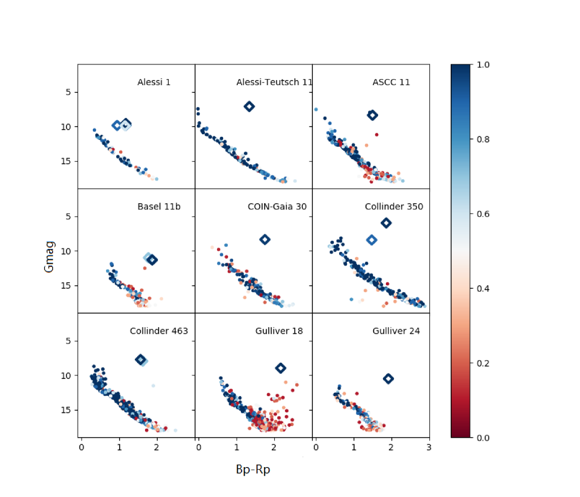
Figure 1: The CMDs of nine of the 18 open clusters; the dots are stars selected from Gaia DR2 database, the large diamonds are targets observed in this work. All points are coloured by membership probability (Cantat-Gaudin et al., 2018).

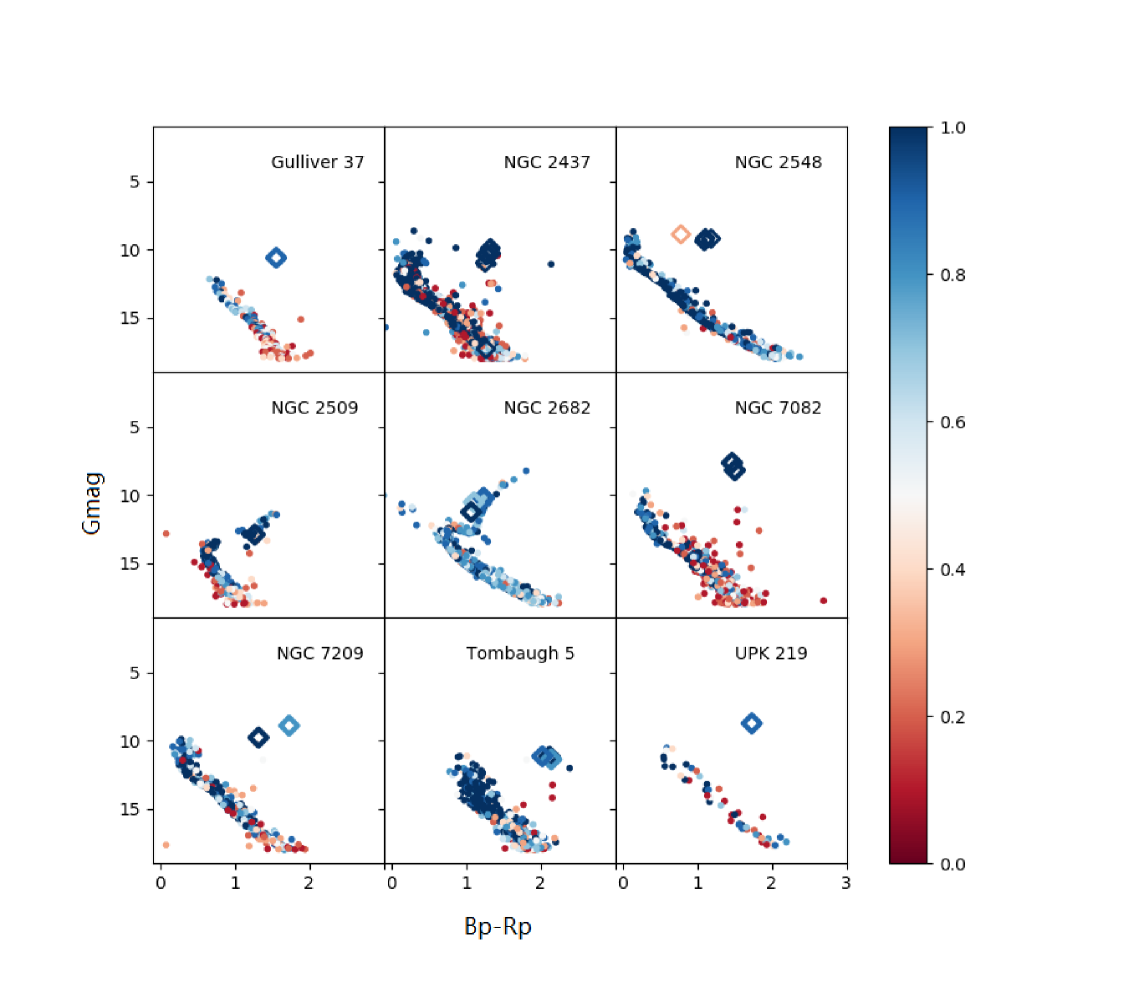
Figure 2: As in the previous figure, for the remaining nine clusters.

Table 1: Properties of the observed clusters.

Cluster	RA	Dec	l	b	logAge	AV	plx	pmRA	pmDE	dist	RGC	—z—
	(J2000)	(J2000)	(deg)	(deg)	(yr)	(mag)	(mas)	(mas yr${}^{-1})$	(mas yr-1)	(pc)	(pc)	(pc)
ASCC 11	03:32:13.44	+44:51:21.6	150.546	-9.224	8.39	0.60	1.141	0.926	-3.030	867	9095	139
Alessi 1	00:53:22.32	+49:32:09.6	123.255	-13.33	9.16	0.08	1.390	6.536	-6.245	689	8726	159
Alessi-Teusch 11	20:16:30.48	+52:03:03.6	87.435	9.268	8.16	0.37	1.520	-0.139	-1.295	634	8335	102
Basel 11b	05:58:11.28	+21:57:54.0	187.442	-1.117	8.36	1.56	0.534	1.046	-4.137	1793	10121	34
COIN-Gaia 30	01:24:19.20	+70:34:26.4	125.684	7.878	8.41	1.25	1.346	-6.145	2.067	767	8804	105
Collinder 463	01:48:07.44	+71:44:16.8	127.391	9.358	8.06	0.79	1.137	-1.715	-0.307	849	8874	138
Gulliver 18	20:11:37.20	+26:31:55.2	65.527	-3.971	7.60	1.59	0.613	-3.198	-5.646	1595	7816	110
Gulliver 24	00:04:38.64	+62:50:06.0	117.62	0.447	8.25	1.05	0.636	-3.241	-1.57	1498	9131	11
Gulliver 37	19:28:18.48	+25:20:49.2	59.547	3.806	8.55	1.33	0.642	-0.775	-3.74	1438	7712	95
NGC 2437	07:41:46.80	-14:50:38.4	231.889	4.051	8.48	0.73	0.603	-3.838	0.365	1511	9345	106
NGC 2509	08:00:48.24	-19:03:21.6	237.844	5.840	9.18	0.23	0.363	-2.708	0.764	2495	9887	254
NGC 2548	08:13:38.88	-05:43:33.6	227.842	15.390	8.59	0.15	1.289	-1.313	1.029	772	8857	205
NGC 7082	21:28:44.64	+47:06:10.8	91.115	-2.859	7.79	0.79	0.729	-0.293	-1.106	1339	8472	66
NGC 7209	22:04:53.76	+46:30:28.8	95.480	-7.296	8.63	0.53	0.820	2.255	0.283	1154	8525	146
Tombaugh 5	03:47:56.16	+59:04:12.0	143.944	3.599	8.27	2.07	0.561	0.515	-2.388	1706	9768	107
UPK 219	23:27:24.96	+65:18:36.0	114.325	3.861	8.17	1.20	1.210	-1.734	-2.459	873	8735	58
Comparison clusters
Collinder 350	17:48:04.32	+01:31:30.0	26.952	14.773	8.77	0.52	2.708	4.965	-0.019	371	8021	94
NGC 2682	08:51:23.04	+11:48:50.4	215.691	31.921	9.63	0.07	1.135	10.986	-2.964	889	8964	470

Table 2: Radial velocities of targets.

Name	Gaia ID	S/N	RV	$\sigma$RV	RV(Gaia)	$\sigma$RV(Gaia)	Notes
		(600nm)	km s-1	km s-1	km s-1	km s-1
ASCC 11	241730418805573760	93	-13.36	0.15	-13.87	0.23
Alessi 1_1	402506369136008832	93	-5.50	0.05	-4.19	0.64
Alessi 1_2	40250599117880752	88	-3.13	0.07	-5.23	0.81
Alessi 1_3	402867593065772288	127	-4.57	0.20	-4.25	1.83
Alessi 1_4	402880684126058880	120	-4.29	0.03	-4.54	0.42
Alessi-Teusch 11	2184332753719499904	126	-27.11	0.12	-27.09	0.17
Basel 11b_1	3424056131485038592	125	2.26	0.18	3.11	0.49
Basel 11b_2	3424055921028900736	86	1.68	0.15	5.81	1.11
Basel 11b_3	3424057540234289408	66	2.57	0.15	2.71	1.12
COIN-Gaia 30	532533682228608384	93	-26.66	0.13	-26.10	0.14
Collinder 463_1	534207555539397888	143	-9.68	0.16	-12.47	0.14
Collinder 463_2	534363067715447680	152	-11.64	0.12	-11.62	0.14
Gulliver 18	1836389309820904064	87	-1.97	0.18	-3.32	0.21
Gulliver 24	430035249779499264	78	-30.37	0.16	-31.86	0.49
Gulliver 37	2024469226291472000	78	-4.59	0.17	2.52	8.22	binary? (see text)
NGC 2437_1	3029609393042459392	64	49.77	0.11	50.07	0.61
NGC 2437_2	3029202711180744832	111	47.16	0.14	46.80	0.50
NGC 2437_3	3030364134752459904	95	49.02	0.17	48.80	0.25
NGC 2437_4	3029132686034894592	128	49.93	0.15
NGC 2437_5	3029156222454419072	50	49.37	0.17	49.34	0.17
NGC 2437_6	3029207006148017664	72	27.12	0.17	28.76	9.91	P$\sim 3350^{d}$ (Mermilliod et al., 2007)
NGC 2437_7	3029226694277998080	74	49.53	0.19	51.60	0.62
NGC 2509	5714209934411718784	128	61.63	0.14	61.42	1.45
NGC 2548_1	3064481400744808704	125	9.06	0.14	8.68	0.29
NGC 2548_2	3064537647636773760	138	8.16	0.03	8.83	0.31
NGC 2548_3	3064579703955646976	77	8.01	0.04	8.76	0.22
NGC 2548_4	3064486692144030336	94	8.98	0.10	8.10	0.67	SB (Mermilliod et al., 2008)
NGC 7082_1	1972288740859811072	144	-11.89	0.15	-11.07	0.19
NGC 7082_2	1972288637780285312	151					Double lined binary
NGC 7209_1	1975004019170020736	81	-19.00	0.16	-18.14	0.27
NGC 7209_2	1975002919658397568	161	-17.98	0.15	-18.89	0.35
Tombaugh 5_1	473266779976916480	72	-23.03	0.15	-22.05	1.03
Tombaugh 5_2	473275782228263296	54	-22.63	0.12	-22.84	0.26
Tombaugh 5_3	473268424940932864	53	-20.53	0.13	-23.45	0.29
UPK 219	2209440823287736064	81	-0.07	0.15	-2.03	0.55
Comparison clusters
Collinder 350_1	4372743213795720704	240	-13.98	0.17	-14.57	0.20
Collinder 350_2	4372572888274176768	70	-16.30	0.13	-14.73	0.16
NGC 2682_1	604921512005266048	141	33.63	0.23	34.29	0.30
NGC 2682_2	604920202039656064	78	34.93	0.14	34.49	0.35
NGC 2682_3	604904950611554432	82	33.93	0.20	36.83	0.96	binary (see Tab. 6)
NGC 2682_4	604917728138508160	53	27.41	0.13	26.98	2.70	binary (see Tab. 6)

2 Target selection and dataset

In this work, we present the analysis of 40 giant stars in 18 open clusters. Sixteen of the OCs were poorly or not at all studied before, while two of them were previously studied and work as comparison samples. These clusters were selected because they are in the Sun vicinity so we could obtain good quality, high-resolution spectra and are old enough to have stars evolved off the main sequence. The target stars were not selected directly from the Gaia DR2 catalog, but from the membership analysis done by Cantat-Gaudin et al. (2018). We targeted only stars with high membership probability and we have from one (in 8 cases) to a maximum of 7 stars (in 1 cluster) per OC.

We selected (almost) only red clump stars, not giants in general. They are a rather homogeneous type of stars, bright enough (their absolute magnitude is $M_{V}\sim 0-1$ mag, Girardi 2016) to be observed at very high-resolution in the Solar neighborhood and to relatively large distance, warm enough ($T_{\textrm{eff}}\sim 4500-5700$ K, Girardi 2016) that they can be analysed to derive meaningful parameters and abundances. Their temperature is high enough to allow a precise abundance analysis, as opposed to cooler, upper red giant branch stars, where line crowding (in particular at near solar metallicities) may hamper accurate analyses (see for instance the discussion in Casali et al. 2020).

Table 1 shows information on the clusters’ position (both equatorial and Galactic coordinates) and some basic parameter, such as age, distance, reddening, etc. All values come from a single homogeneous source, i.e. Cantat-Gaudin et al. (2020), where Gaia DR2 data are used to define candidate cluster members and derive cluster properties (see that paper for details).

All these OCs are located in the Galactic thin disc, cover the Galactocentric distance range 7.7-10 kpc, reside close to the Galactic midplane, and are in the age range from about 50 Myr to 4 Gyr. Figures 1, 2 show the colour-magnitude diagrams (CMD) in the Gaia system of the 18 OCs, based on the selection of Cantat-Gaudin et al. (2018); the stars are coloured with membership probability and the observed targes are indicated by larger symbols.

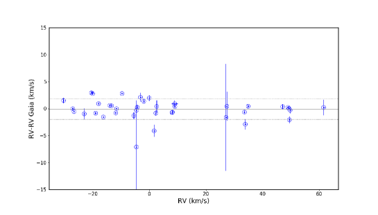
Figure 3: Difference in radial velocities for targets between Gaia and this work. The error of our sample is shown in the x-axis (it is so small that it falls within the symbol), and only the Gaia error is plotted on the y-axis, as it is much larger. The grey lines indicate the mean value of offset $-0.11\pm 1.9$ km s^-1 (standard deviation).

3 Observation, data reduction and radial velocities

Observations were carried out in four observing runs in December 2018, January, August, and December 2019. In most cases, multiple exposures were obtained (see Table LABEL:tab:A1 for details on the individual targets). The exposure times varied according to the star magnitude and the sky conditions; the goal was to reach at least a signal-to-noise ratio (S/N) of 50 at 500nm. We combined multi-exposure spectra before further data analysis.

All of those data were obtained with the 3.5 m Telescopio Nazionale Galileo (TNG) at El Roque de los Muchachos Observatory (La Palma, Canary Islands, Spain). We used the two high-resolutions spectrographs HARPS-N and GIANO in GIARPS mode. This means that observation in the optical range and near-IR are executed at the same time, with the light from a single target separated using a dichroic (a few more details can be found in previous SPA papers, see e.g. Frasca et al., 2019; D’Orazi et al., 2020). The analysis of GIANO data will be presented in forthcoming works; we deal here with the HARPS-N data. HARPS-N covers the wavelength range between 383 and 693 nm, with resolution R = 115000; this spectrograph is very well suited for determining radial velocity (RV) and abundances with very high precision.

The spectra were reduced by the HARPS-N Data Reduction Pipelines (they were corrected for bias, flat field, extracted to 1d spectra, wavelength calibrated and corrected for barycentric motion) and retrieved from the Italian Center for Astronomical Archives in Trieste (http://ia2-harps.oats.inaf.it/). Spectrum continuum normalization with cubic splines and combination were done with IRAF using the tasks continuum, scombine.

The calculation of RV was done on the final normalized spectra with the IRAF task rvidlines, which measures the wavelength shift of a list of features. For all stars, the RV information and the error is given in Table 2, together with the S/N measured at 600 nm. As we selected high probability members, we find very similar RVs for stars belonging to the same cluster, which further reinforces their membership.

All our stars except one (plus the binary) have an RV determined with the RVS instrument on board Gaia, which observes the near-IR Ca ii triplet region at resolution R=11500. These RVs and the corresponding errors, from Gaia DR2, are also presented in Table 2.

Figure 3 shows the distribution of RV offsets between the value determined in this work and that from Gaia. These offsets are generally small with an average offset of $-0.11\pm 1.89$ km s^-1. Owing to our small sample we have not performed further comparison.

The few discrepant values seem probably due to the much larger errors in the Gaia RVS determinations or to binarity. Two stars in NGC 2682, namely 3 and 4 in our list, one in NGC 2437, namely 6 in our list, and one in NGC 2548, namely 4 in our list, are known binaries (Mermilliod et al., 2007, 2008; Geller et al., 2021). The only Gulliver 37 star observed shows a large Gaia RV dispersion, 8.2 km s^-1 based on 11 transits, with an average RV of 2.5 km s^-1, compared to our value of -4.59 km s^-1. Moreover, we have in hand an optical high resolution spectrum for another project from which we derived a RV of $21.92\pm 0.02$ km s^-1 (Carrera et al. in prep.). Due to the large velocity dispersion reported by Gaia and the discrepancy among the different radial velocity determinations, we consider it as a probable spectroscopic binary. All these stars do not present doubling of their lines, so the measure of the atmospheric parameters is negligibly affected by the presence of any unseen companion with respect to the precision of our analysis.

4 Stellar Parameters

Atmospheric parameters were determined spectroscopically, minimizing abundance trends with excitation potential, strength of the line and imposing ionisation equilibrium. In this section we describe this procedure.

4.1 Line list and Equivalent Width measurement

We adopted the line list for Fe i from Ruffoni et al. (2014) and Fe ii from Meléndez & Barbuy (2009), selecting the lines in the 430 to 640  nm interval. HARPS-N spectra start from 383  nm; however, the S/N is quite low in that region for our spectra. This fact, combined with the extreme crowding of features in the blue part of the spectrum, led us to discard all Fe lines bluer than 430  nm, as their intensity could not be measured with the same accuracy of those in redder regions.

Equivalent widths (EWs hereafter) were measured with the code ARES, following the procedure described in Sousa et al. (2015), using a S/N dependent approach to set the local continuum. Visual inspection was performed for very strong lines (EW $>150$mÅ) and lines with large fitting errors (EW ¡ 3$\times\sigma$(EW)) and we performed a manual measurement of the EW using IRAF splot when the inspection showed an issue with the ARES fitting (e.g. incorrect continuum placing due to a badly subtracted cosmic ray). Lines which turned out to be blended were discarded.

4.2 Photometric Parameters

The determination of the atmospheric parameters requires a set of initial parameters to be used in the first iteration of the abundance analysis determination. For this purpose, we used photometric parameters, that are determined on the basis of observed photometric colour(s) and the latest generation of stellar isochrones.

To determine the initial stellar effective temperature ($T_{\textrm{}eff}$) we used IRFM (Infrared flux method). This method is model independent and relies on the flux on the stellar surface in infrared wavelength which relates to the surface temperature. We derived the J-K colours from 2MASS, applied the appropriate reddening for the target coordinate as derived from IRSA (Schlafly & Finkbeiner, 2011). The computation of photometric surface temperature follows the colour-temperature polynomial fitting based on a sample of F0-K5 type from Alonso et al. (1999), appropriate for stars in the range 3700-5300 K, which is consistent with our sample.

To determine $\log g$ we used Padova CMD isochrones (PARSEC release v1.2s, Marigo et al. 2017 and COLIBRI, Pastorelli et al. 2020, and references therein), with web interface CMD 3.4.

For age and metallicity input for the isochrones we used information taken from the literature (see Table 1). In case no estimate of metallicity was available, we adopted the average metallicity of the thin disc ([Fe/H] = -0.25dex Soubiran et al. 2003). This is admittedly low for the typical OC, however it has a negligible impact on the final parameters in Table 3.

In fact, while it is important to provide reasonably accurate input parameters in the isochrones to derive similarly reasonable photometric parameters, these values are just the starting point to build the initial model atmosphere. The actual atmospheric parameters have been determined on the basis of the observed spectra (see next section).

Table 3: Initial parameters from photometric data.

Name	$T_{\textrm{eff}}$	$\log$ g	[Fe/H]	vmicro
	(K)	(dex)	(dex)	(km s-1)
ASCC 11	4867	2.36	-0.25	1.0
Alessi 1_1	4677	2.39	-0.25	1.0
Alessi 1_2	4600	2.28	-0.25	1.0
Alessi 1_3	4804	3.50	-0.25	1.0
Alessi 1_4	4578	2.25	-0.25	1.0
Alessi-Teusch 11	4790	3.40	0.10	1.0
Basel 11b_1	6259	1.70	0.01	1.0
Basel 11b_2	5917	1.59	0.01	1.0
Basel 11b_3	5693	1.83	0.01	1.0
COIN-Gaia 30	5231	1.70	-0.25	1.0
Collinder 463_1	4730	2.12	-0.25	1.0
Collinder 463_2	4730	2.30	-0.25	1.0
Gulliver 18	4598	1.50	-0.25	1.0
Gulliver 24	4567	1.62	-0.25	1.0
Gulliver 37	5095	1.80	-0.25	1.0
NGC 2437_1	4792	2.24	0.00	1.0
NGC 2437_2	5218	3.38	0.00	1.0
NGC 2437_3	5206	3.38	0.00	1.0
NGC 2437_4	5087	2.39	0.00	1.0
NGC 2437_5	4990	2.37	0.00	1.0
NGC 2437_6	4848	2.29	0.00	1.0
NGC 2437_7	4549	1.95	0.00	1.0
NGC 2509	4705	2.27	0.00	1.0
NGC 2548_1	5114	2.50	-0.24	1.0
NGC 2548_2	5047	2.27	-0.24	1.0
NGC 2548_3	4853	2.35	-0.24	1.0
NGC 2548_4	5327	2.70	-0.24	1.0
NGC 7082	4994	1.56	-0.01	1.0
NGC 7209_1	4799	2.50	0.01	1.0
NGC 7209_2	4142	1.50	0.01	1.0
Tombaugh 5_1	5024	2.42	0.06	1.0
Tombaugh 5_2	5021	2.40	0.06	1.0
Tombaugh 5_3	5270	2.44	0.06	1.0
UPK 219	5203	3.01	-0.25	1.0
Comparison clusters
Collinder 350_1	4200	1.30	0.10	1.0
Collinder 350_2	5300	3.20	0.10	1.0
NGC 2682_1	4537	3.61	0.00	1.0
NGC 2682_2	4601	2.50	0.00	1.0
NGC 2682_3	4823	2.90	0.00	1.0
NGC 2682_4	4967	3.36	0.00	1.0

4.3 Spectroscopic Parameters

The atmospheric parameters analysis was performed using the code MOOG (used through the python wrapper pymoogi, based on the MOOG 2019 version), a 1D, Local Thermodynamic Equilibrium (LTE) stellar line analysis code. The model atmospheres were calculated interpolating the ATLAS9 stellar atmosphere library (Castelli & Kurucz, 2003) in 1D plane-parallel geometry. While in principle spherical models should be better for giants, in practice this choice does not introduce significant differences (Casali et al., 2020, see e.g.).

Atmospheric parameters were determined iteratively, by varying their values in the input model atmosphere until excitation and ionisation equilibria were reached.

In other words, $T_{\textrm{eff}}$’s and microturbulent velocities ($v_{micro}$) were determined by minimising the trends of Fe I abundance as determined from different lines as a function of their excitation potential and their intensity, respectively; surface gravity was determined by matching (within the errors) output Fe I and Fe II abundances. While we adopt the solar abundances from Grevesse & Sauval (1998), we have also repeated the procedure for a solar spectrum collected with HARPS-N during one of our runs, finding an Fe abundance essentially identical to that reported in Grevesse & Sauval (1998). Errors on the atmospheric parameters were derived following the same procedure outlined in Epstein et al. (2010).

The resulting atmospheric parameters along with their associated uncertainties are reported in Table LABEL:tab:A2 for all individual targets. The mean value of metallicity for each cluster is quoted in Table 5 (where, for Collinder 350, we use only the warmer star).

Table 4: Mean RV and metallicity for the observed clusters.

Cluster	RV	$\sigma$RV	[Fe/H]	$\sigma$[Fe/H]	N
	(km s-1)	(km s-1)	(dex)	(dex)
ASCC 11	-10.94	0.19	-0.14	0.05	1
Alessi 1	-4.37	0.85	0.00	0.08	4
Alessi-Teusch 11	-27.11	0.12	-0.19	0.05	1
Basel 11b	2.17	0.37	-0.01	0.05	3
COIN-Gaia 30	-26.66	0.13	0.03	0.05	1
Collinder 463	-10.66	0.98	-0.15	0.05	2
Gulliver 18	-1.97	0.18	-0.10	0.05	1
Gulliver 24	-30.37	0.16	-0.10	0.05	1
Gulliver 37	-4.59 a	0.17	0.10	0.05	1
NGC 2437	49.13a	0.93	0.00	0.04	7
NGC 2509	61.63	0.14	-0.10	0.06	1
NGC 2548	8.41a	0.46	-0.02	0.03	4
NGC 7082	-11.89	0.15	-0.15	0.05	1
NGC 7209	-18.49	0.51	-0.04	0.04	2
Tombaugh 5	-21.21	1.30	0.05	0.05	3
UPK 219	-0.07	0.15	0.02	0.05	1
Comparison clusters
Collinder 350	-15.14	1.16	0.00	0.05	1
NGC 2682	34.28a	0;65	0.03	0.03	4

4.4 Comparison with literature

Two clusters, namely Collinder 350 and NGC 2682 (M67) have been included in the present sample for comparison purpose. The former has been investigated in a previous SPA paper (Casali et al., 2020), which reports results obtained with a slightly different approach for the same stars, therefore allowing the mapping of possible offsets. The latter, NGC 2682, is one of the most studied OCs and represents an ideal benchmark cluster. A few more clusters have some recently published analyses. One of them was purposely observed (Tombaugh 5) as the existing spectra were of moderate-resolution; for two more (Basel 11b, NGC 2548) the results were published after our observations had already been taken. Finally, we note that some other clusters (ASCC 11, Alessi-Teusch 11, Collinder 350, NGC 2548, and NGC 2682) were observed within the LAMOST survey, at R=1800 (Zhang et al., 2019). However, we will not discuss this last case, limiting comparisons only to spectra with at least moderate resolution (R$>10000$).

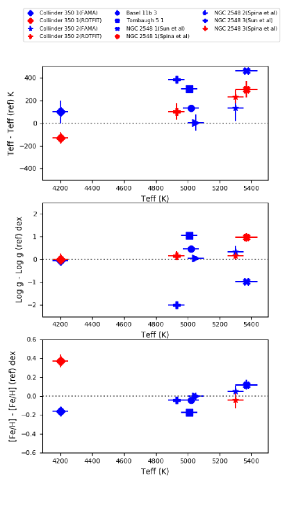
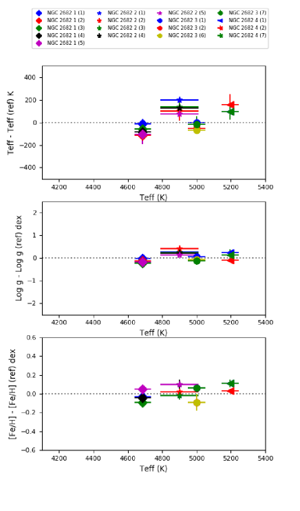
Figure 4: Comparison of atmospheric parameters for targets with high resolution spectroscopic determinations. We plot out $T_{\textrm{eff}}$ in the x axis and the difference (our minus literature) and the error from literature on the y-axis. In the right column we show the different sources in NGC 2682 and in the left column all other clusters. Ref: (1) Jacobson et al. (2011); (2) APOGEE DR16; (3) (Casamiquela et al., 2017) EW; (4) Casamiquela et al. (2017) SS; (5) Gao et al. (2018); (6) Luck (2015);(7) Spina et al. (2021)

We give details below and briefly summarise how our results compare to literature. In particular, Fig. 4 gives a visual comparison, while Tab. 6 presents detailed values for the benchmark cluster NGC 2682 and the other stars. We remark that, for NGC 2682, there are no systematic differences among the different studies.

Collinder 350 -

In our sample, we collected and analysed spectra for two members of Collinder 350, one of the least studied open clusters in the solar neighborhood. For the coolest star (4200 K) we obtained [Fe/H]=$-0.40\pm 0.08$ dex, while for the hottest (5300 K) we found [Fe/H]=$0.00\pm 0.05$ dex. In the work of Blanco-Cuaresma & Fraix-Burnet (2018), the metallicity was estimated at 0.03 dex from the spectrum of one single star with a resolution about 80,000. In the SPA paper by Casali et al. (2020), the value of [Fe/H] was measured using two methods on the same stars as in our analysis. Even in this case the two stars show a difference in the measured metallicity, even if smaller than in the present analysis. With ROTFIT (i.e. fitting of spectral libraries) they get $0.03\pm 0.07$ dex (cooler star) and $-0.02\pm 0.09$ dex (hotter star) while with FAMA (i.e. automatic method based on EWs analysis) they derive $-0.24\pm 0.02$ dex (cooler star) and $-0.03\pm 0.06$ dex (hotter star).

Comparing to the present paper, the results are overall in fair agreement. The hotter star shows [Fe/H]=0, a value consistent with that from both methods in Casali’s work. For the cooler star, our result is more metal poor than that measured by Casali’s paper using either method. As mentioned by Casali et al. (2020), we believe that at such temperature the placements of the continuum is challenging in these stars, as they are very rich in absorption lines, leading to the less accurate metallicities for star with low temperature ($T_{\textrm{eff}}$ ¡ 4300 K, $log$ g ¡ 1.8 dex).

NGC 2682 (M67) -

This is one of the most studied open clusters and has solar metallicity and age (see e.g. Bertelli Motta et al., 2018; Bossini et al., 2019). We observed four stars, two on the red clump and single, and two red giants known to be binary systems (see Tables 2 and 6). In particular, the two single-lined binaries (stars 3, 4 in our list) were studied by Mermilliod et al. (2007, 2008) and Geller et al. (2021), who derived their orbital parameters. Star NGC 2682 3 (aka S1237) is a yellow straggler (Leiner et al., 2016), i.e. a star falling between the blue stragglers (BSS) and the red giants, above the subgiant branch level in optical CMDs. Leiner et al. (2016) used Kepler K2 data to derive a mass of 2.9$\pm$0.2 M_⊙, about twice the mass of turn-off stars, corroborating the notion that yellow stragglers are a later evolutionary phase of BSS. We collected results of spectral analysis from multi-work and list them in Table 6. The parameters are in overall good agreement with the literature.

Table 5: Comparison of atmospheric parameters with literature.

star	$T_{\textrm{eff}}$	$\sigma T_{eff}$	log g	$\sigma$log g	[Fe/H]	$\sigma$[Fe/H]	Reference	Notes
	(K)		(dex)		(dex)
NGC 2682_1	4687	50	2.37	0.07	-0.05	0.05	Present study	RC, single
	4700		2.40		-0.02		Jacobson et al. (2011)
	4803	84	2.48	0.04		0.01	APOGEE DR16
	4745	57	2.59	0.09	0.04	0.04	Casamiquela et al. (2017) EW
	4771	13	2.55	0.03	-0.04	0.05	Casamiquela et al. (2017) SS
	4793		2.55		-0.10		Gao et al. (2018)
NGC 2682_2	4900	110	2.76	0.10	0.02	0.05	Present study	RC, single
	4700		2.50		0.04		Jacobson et al. (2011)
	4802	84	2.34	0.04	0.00	0.01	APOGEE DR16
	4762	37	2.53	0.07	0.04	0.04	Casamiquela et al. (2017) EW
	4776	13	2.54	0.03	-0.08	0.05	Casamiquela et al. (2017) SS
	4824		2.62		-0.08		Gao et al. (2018)
NGC 2682_3	5000	50	2.77	0.10	-0.03	0.03	Present study	SB1, $P\sim 700^{d}$ (Geller et al. 2021),
	5000		2.70		-0.09		Jacobson et al. (2011)	yellow straggler (Leiner et al. 2016)
	5056		2.85		0.06	0.09	APOGEE DR16
	5067		2.85		0.06	0.09	Luck (2015)
	5018	71	2.88	0.19	-0.09	0.04	Spina et al. (2021)
NGC 2682_4	5195	50	3.25	0.10	0.00	0.05	Present study	SB1, $P\sim 43^{d}$ (Mermilliod et al. 2007;
	5100		3.00		-0.11		Jacobson et al. (2011)	Geller et al. 2021)
	5040	92	3.34	0.06	-0.03	0.01	APOGEE DR16
	5098	71	3.12	0.26	-0.11	0.04	Spina et al. (2021)
Collinder 350_1	4200	50	1.30	0.20	-0.40	0.08	Present study
	4100	100	1.35	0.23	-0.24	0.01	Casali et al. (2020) FAMA
	4330	50	1.28	0.24	-0.03	0.07	Casali et al. (2020) ROTFIT
Collinder 350_2	5300	50	3.15	0.10	0.02	0.05	Present study
	5170	110	2.85	0.27	-0.03	0.06	Casali et al. (2020) FAMA
	5070	60	2.99	0.19	-0.02	0.09	Casali et al. (2020) ROTFIT
Basel 11b_3	4950	50	2.83	0.10	-0.04	0.05	Present study
	4817	86	2.37	0.04	0.00	0.01	APOGEE DR 16	2M05581816+2158437
Tombaugh 5_1	5010	50	3.17	0.15	0.04	0.05	Present study
	4710		2.10		0.21	0.05	Baratella et al. (2018)
NGC 2548_1	5370	70	3.67	0.15	0.00	0.05	Present study
	4912		4.64				Sun et al. (2020)
	5074	73	2.69	0.19	-0.12	0.05	Spina et al. (2021)
NGC 2548_2	5050	50	2.65	0.10	-0.02	0.04	Present study
	5049	72	2.59	0.10	-0.02	0.04	Spina et al. (2021)
NGC 2548_3	4930	50	2.70	0.10	-0.01	0.05	Present study
	4549		4.69				Sun et al. (2020)
	4829	72	2.53	0.19	0.03	0.04	Spina et al. (2021)

Tombaugh 5 -

A metallicity estimate based on moderate-resolution spectroscopy also exists for Tombaugh 5. Baratella et al. (2018) reported atmospheric parameters (from mid-res spectra, R=13 000) for five members out of seven observed. In this case two stars are in common with our sample, as they were targeted on purpose. However, only one (Tombaugh 5_1 for us, 7701 in Baratella et al. 2018) is analyzed in both papers, as they considered the second (Tombaugh 5_2 for us, 8099 in Baratella et al. 2018) a possible non member on the basis of its RV and previous literature. The latter star has a high probability of being a member according to Cantat-Gaudin et al. (2018) and the RVs measured by us and Gaia RVS upport its membership. In Baratella et al. (2018) temperature and gravity were derived spectroscopically and abundances were measured using EWs, with estimated errors of 0.15-0.20 dex. They found an average metallicity of 0.06 $\pm$ 0.11 dex. The mean value from our analysis is 0.05 $\pm$ 0.05 dex. The agreement between the analyses for all atmospheric parameters is reasonable, given the large difference in resolution between the data sets (see Fig. 4).

NGC 2548 -

A recent paper Sun et al. (2020) is based on moderate-resolution spectra. They report the radial and rotational velocities for nearly 300 stars in NGC 2548 (M48), measured with Hydra@WIYN spectra (R$\sim$13500) in a region about 40 nm wide, around the Li i 670.8 nm line. The candidate cluster stars were selected from CMDs based on UBVRI photometry and about two thirds resulted member, both single or in binary/multiple systems, combining the spectroscopic data and Gaia DR2 results. Temperature and gravity were derived from photometric data. For a subsample of 99 well behaved, low rotational velocity, single cluster members, the value of the metallicity was derived using 16 Fe i lines, finding an average metallicity [Fe/H]=$-0.06\pm 0.007$ dex. This is in agreement with $-0.02\pm 0.04$ dex from 4 stars in our work.

Two stars are in common, for which Sun et al. (2020) report $T_{\textrm{eff}}$’s of 4912 K and 4549 K, with $\log g$ 4.64 and 4.69 respectively. We obtained $T_{\textrm{eff}}$’s 5370$\pm$110 K and 4930$\pm$60 K and our values for $\log g$ are much lower, 3.67$\pm$0.1 dex and 2.68$\pm$0.05 dex respectively, consistent with the stars being evolved rather than in the main sequence. The gravities in Sun et al. (2020) are derived using the Yale-Yonsei isochrones, an approach that leads to two possible solutions, corresponding to an evolved or a main sequence star. Sun et al. (2020) adopted the dwarf solution, and the reason behind this choice is not discussed in the paper. However, given the position on the CMD of the observed stars (see Fig. 2), we expect that the solution corresponding to an evolved (and thus brighter) star is the most appropriate one.

Basel 11b -

Finally, among the 128 OCs published in Donor et al. (2020) and based on SDSS/APOGEE DR16, there is Basel_11b. The paper presents the metallicity based on one single star, [Fe/H]=0. For this star we determined [Fe/H]=-0.04 and the mean iron abundance, based on 3 stars, is of $-0.013\pm 0.034$ dex. Further comparison of atmospheric parameters is found in Tab. 6.

5 Discussion

The average metallicities for our sample of OCs are given in Tab. 5. These are combined with the clusters positions (in the following, Galactocentric distance and height on the plane) to discuss the metallicity distribution in the disc, adding literature data to increase the sample and the coverage of disc properties.

5.1 Metallicity distribution in the disc

The study of the radial and vertical fossil gradients such as age and composition is one of the main approaches in probing the Galactic disc(s).

In this section, we discuss the observed behaviour of OCs’ metallicity, age and Galactocentric distance and what information can be gained by the comparison with models for the disc. First we derive the classical radial gradient in metallicity (e.g. Friel et al. 2002), then we compare observations with models. Our sample is distributed essentially on the Galactic plane, the SPA clusters are all within 0.5 kpc (Cantat-Gaudin et al., 2020), and generally in the solar neighbourhood, with Galactocentric distance ranging between 7.7 to $\sim$10 kpc. With one single exception – NGC 2682, which was observed for comparison purposes – the clusters are quite young, with 14 out of 18 clusters being younger than 0.5 Gyr.

By combining our data with results from some selected surveys and studies, we can widen the sample to clusters with larger ages and/or distances from the Galactic centre, building a sample that allows us to probe the properties of the Galactic disc, and can be used to constrain models of the chemo-dynamical evolution of the disc. The SPA sample currently includes the present analysis as well as four more OCs in Casali et al. (2020), one from D’Orazi et al. (2020), and another one in Frasca et al. (2019). We include the results from the large spectoscopic surveys, namely: a) APOGEE (Donor et al., 2020), with more than 120 OCs, mostly in the 6-15 kpc range in R_gc and with [Fe/H] from -0.5 to 0.4 dex; b) GES, covering the wide range of Galactocentric distance from 5.8 to 20 kpc, and the metallicity range -0.5 to 0.4 dex; c) and GALAH (Spina et al., 2021), keeping only clusters whose parameters are based on HERMES spectra and excluding those based on the recalibration of APOGEE (see Spina et al. 2021 for details). Moreover, we include the OCCASO sample (Casamiquela et al., 2017), whose OCs are located at Galactocentric distances similar to those of the SPA project (6.5 to 10.5 kpc) and with metallicities around the solar value, ranging from $-$0.1 dex to 0.17 dex.

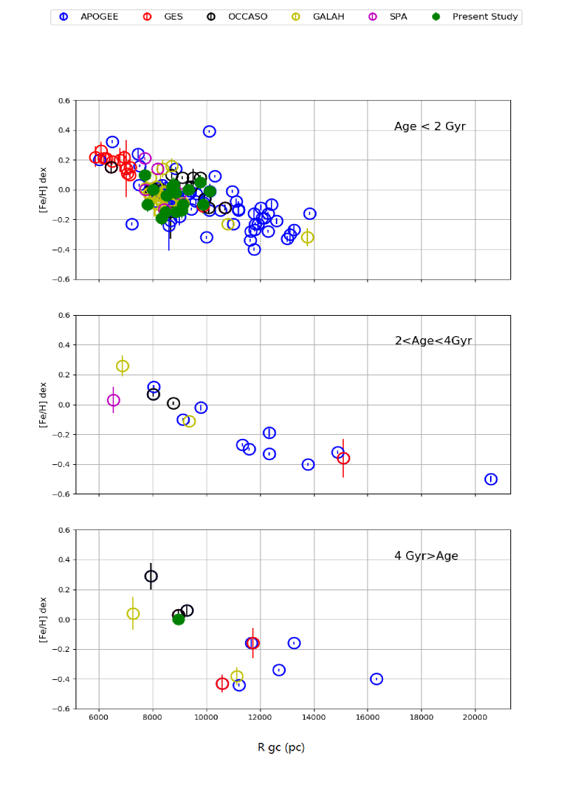
Figure 5: The distribution of metallicity with Galactocentric distance in three age bins (the same used in Minchev et al. 2014, see Sec. 5.2). Beside our clusters, we show data from APOGEE (Donor et al., 2020), GES (Casali et al., 2019), OCCASO (Casamiquela et al., 2017),and GALAH (Spina et al., 2021) plus SPA results already published (Frasca et al., 2019; Casali et al., 2020; D’Orazi et al., 2020).

The relationship between metallicity and Galactocentric distance, classically called metallicity gradient, is shown in Fig. 5 for the combined sample, dividing it in three age intervals (selected because they are the same in Minchev et al. 2014b, see below). The metallicities come from the cited sources (averaging values when more than one was available for a given cluster) and the R_gc values come from Cantat-Gaudin et al. (2020) where R_gc,Sun=8.34 form Reid et al. (2014). Table 6 contains the corresponding gradients, for the whole sample and separated in age bins. As the slope shows a change at about R_gc =14 kpc, we use that limit for inner/outer regions. The same was done in past works, as can be seen from Tab. 8, where we list some selected literature papers. We show the values in Friel et al. (2002), since this is possibly the first analysis of an homogeneous and large spectroscopic sample, albeit based on low resolution spectra, and in a few recent papers. As every work uses different age bins and R_gc ranges, we can make only a qualitative assessment of the results. However, the values in the two tables compare generally well; a few discrepant values are commented in the notes of Tab. 8.

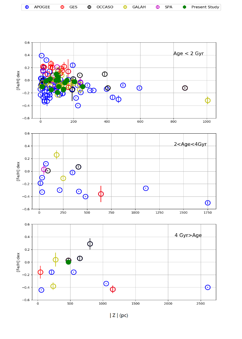
Figure 6: The distribution of metallicity with distance from mid-plate in three age bins (the same used in Minchev et al. 2014, see Sec. 5.2). Beside our clusters, we show data from APOGEE (Donor et al., 2020), GES (Casali et al., 2019), OCCASO (Casamiquela et al., 2017),and GALAH (Spina et al., 2021) plus SPA results already published (Frasca et al., 2019; Casali et al., 2020; D’Orazi et al., 2020).

Figure 6 shows metallicity as a function of distance from the Galactic plane, divided in age bin like the previous figure. The calculated values are listed in Table 6 as well. Note that, overall, the trends with $|z|$, even in well populated bins (e.g. young clusters in the inner disk), is far less statistically relevant than the corresponding slope wrt galactic radius.

We also explored possible residual azimuthal gradient (only for well populated bins), finding extremely weak and moderately significant trends. For the overall sample within 14 kpc, we found 0.0028$\pm$0.0007, while for the sample below 2 Gyr within the same radius we found 0.0022$\pm$0.0009.

Table 6: Observed slope of the metallicity gradient.

Age	Rgc	d[Fe/H]/dRGC	d[Fe/H]/d$|z|_{GC}$	Nclusters
(Gyr)	(kpc)	(dex kpc-1)
all ages	Rgc¡14	-0.066$\pm 0.005$	$-0.249\pm 0.062$	157
all ages	Rgc¿14	-0.032$\pm 0.007$	$-0.040\pm 0.028$	4
age¡2	Rcg¡14	-0.059$\pm 0.006$	$-0.236\pm 0.119$	133
2¡age¡4	Rgc¡14	-0.089$\pm 0.007$	$-0.195\pm 0.144$	13
age¿4	Rgc¡14	0.008$\pm 0.041$	$0.081\pm 0.117$	11

5.2 Comparison with chemo-dynamical models

It must be kept in mind that the chemo-dynamical evolution of the Galactic disc(s) is a rather complex process and the expectation is that much of the initial information will be diluted through the dynamical evolution and radial mixing of the disc. This is expected to affect differently populations of different ages: broadly speaking, the older a cluster is, the more it has undergone dynamical evolution and radial mixing, even if other factors come into play, like the details of the formation environment and more in general the shape and mass of the disc at the time of formation and early evolution.

Recent models for the Galactic thin disc, e.g. Minchev et al. (2013, 2014a, 2014b), taking into account sophisticated simulations in the cosmological context (Martig et al., 2009, 2012) along with a detailed knowledge of the chemical evolution of the disc have been able to generate theoretical gradients to compare with the observations at different ages. However, uncertainties exist, also due to model assumptions (e.g. initial gradient of chemical abundance), especially with regard to the oldest clusters and those furthest from the Galactic plane, which have undergone a large amound of dynamical evolution during their lives.

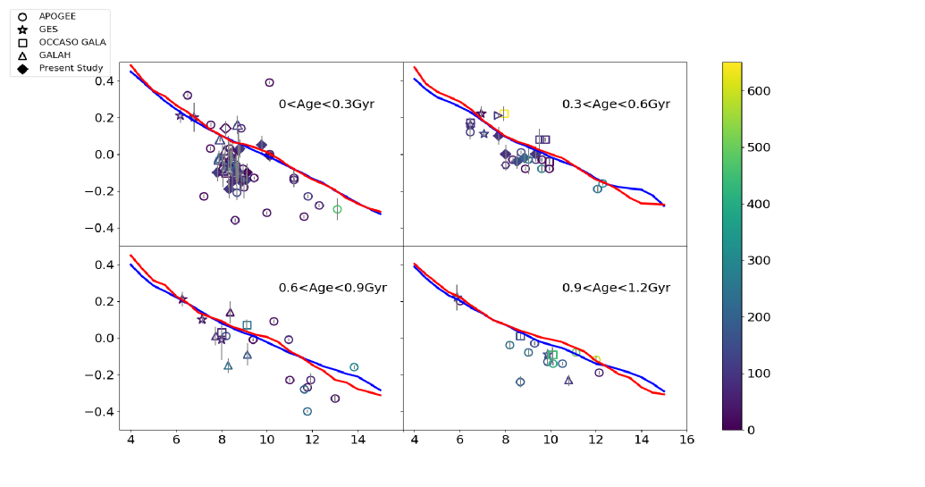
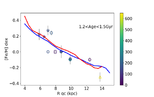
Figure 7: Comparison between model predictions (Minchev et al., 2014a, b) and observation for young clusters. The red and the blue lines are predictions from the MCM models for $|z|<0.3$ kpc and 0.3 $<|z|<$0.8 kpc respectively. The colours in the symbol indicates the distance from the Galactic plane. All considered clusters are within 0.6 kpc from the Galactic plane, with SPA clusters being all within 0.5 kpc. The open ’diamond’ in the first panel is ASCC 123 (Frasca et al., 2019) and the ’triangle’ symbol in 0.3-0.6 Gyr range is NGC 2632 (D’Orazi et al., 2020) The fit is generally good for clusters older than 0.3 Gyr, but the predictions fail to reproduce the data among the very young clusters (see text).

Minchev et al. (2014a) provide gradients calculated for different age intervals and ranges of distance from the Galactic plane. Figure 7 shows the comparison between the combined sample predictions from chemo-dynamical thin-disc model by (Minchev et al., 2014, the so-called MCM model). These models are calculated taking into account cosmological and dynamical properties, and chemical evolution, combining the effects of migration, the distance above the disc midplane, and then extending the model beyond the solar neighborhood. Furthermore, the uncertainties of observation, and the evolution of Galactic disc was considered. From the MCM models we consider the range 0-0.8 kpc in terms of distance from the Galactic plane, which is appropriate for clusters in SPA, but also for the vast majority of the literature sample. We plot the predictions for both $|z|<0.3$ kpc and for 0.3 kpc$<|z|<$0.8 kpc.

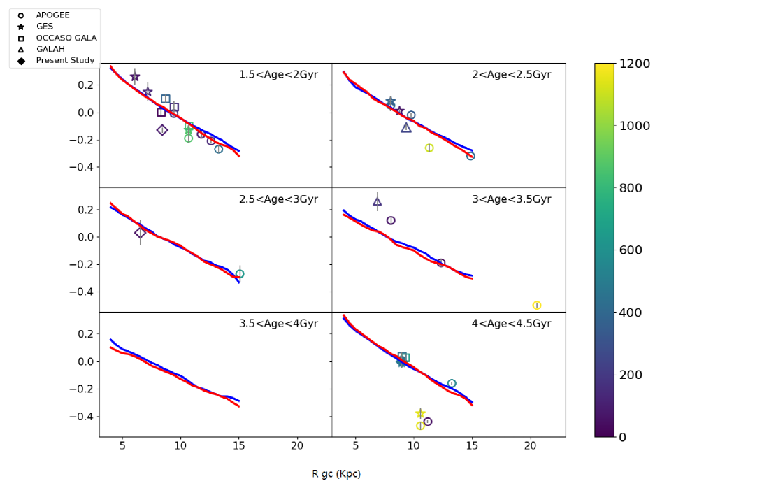
Figure 8: As in Fig. 7 for clusters bewteen 1.5 and 4.5 Gyr. Note the paucity of OCs older than 2.5 Gyr (in particular, only one SPA cluster is present, Ruprecth 171, from Casali et al. 2020). The data are quite well reproduced by the models; the exceptions are the old and very metal poor clusters which have $|z|$ ¿ 1 kpc, further away from the Galactic plane than the plotted models.

Figures 7 and 8 show the comparison between MCM predictions and results from observation data, grouped according to age in bins of 0.3 and 0.5 Gyr, respectively, up to 4.5 Gyr. Predictions are generally a good match for the observation in the age range from 0.3 Gyr to 4.5 Gyr. It is worth noting that in the oldest age bin, two of the three discrepant clusters have —z—$>1$ kpc, larger than the range the models have been calculated for, while the third has a metallicity based on one single star. On the other hand, in the youngest bin the fitting is very poor, even if the clusters lie closer than 0.5 kpc from the Galactic plane; we will come back to this problem later. For a more quantitative comparison with the Minchev et al. (2014b) results we derived the gradients in our sample following the bins in age and Z in their Table 1, considered the error of metallicities in the fitting process. We employed their same separations in R_gc and [z] and computed the corresponding gradients for the observed sample. Interestingly, the gradient computed for age younger than 2 Gyr and —z— ¡ 0.25 kpc, i.e. the bin comprising the vast majority of our sample (97 OCs), is comparable to that from the prediction: $-0.066\pm 0.008$ versus -0.057 for observed and predicted slope, respectively (see below, however, for a caveat on the very young clusters). Values are instead different in the other bins, which are, however, very scarcely populated, so it is difficult to assess if the discrepancy is important.

Coming back to the very different distribution of OC metallicity for young ages (already noticed in past work, e.g. Spina et al. 2017), several possible factors might be the source(s) of the poor fit. On the observational side, inaccurate measurements of the parameters could cause the issue. For example, a systematic underestimate in the Galactic distances would lead to outer disc clusters being compared to solar neighborhood predictions. A systematic underestimate in Z, on the other hand, would mean that we would be using predictions unsuitable for the sample. R_gc and Z are based on Gaia DR2 data, with typical uncertainties of around 5% to 10% for distance (Cantat-Gaudin et al., 2020), which is not large enough to generate the observed effect. Moreover, if such a systematic errors existed, they would very likely affect similarly clusters in the other age bins, a phenomenon of which there is no evidence. We note that a systematic error in the adopted age could not in any way explain the poor fit: the discrepant clusters with $<0.3$ Gyr would not be reproduced by predictions of any of the plotted ages.

Another possibility is that (part of) the metallicities we are using in the plot are not enough accurate. In particular we have checked in more detail APOGEE cluster from Donor et al. (2020). Firstly, we have detected that for several cluster there are significant difference between the two latest data releases, DR16 (Donor et al., 2020) and DR14 (Donor et al., 2018; Carrera et al., 2019), even if the same stars are used in both cases. This is for instance the case of King 7, with [Fe/H]=-0.13$\pm$0.05 and -0.04$\pm$0.01 in DR16 and DR14, respectively. These differences may be explained by the different methodologies used in the two releases to obtain the final abundances (see Jönsson et al., 2018, 2020, for a detailed explanation). For several clusters the values are based only on a single star with either low astrometric membership probability from Cantat-Gaudin et al. (2018), e.g. Berkeley 79, Czernik 23, FSR 852, King 12, NGC 1857 and/or with discrepant radial velocities in comparison with the literature, e.g. Czernik 23, NGC 2311, NGC 6383. Additionally, the star observed in NGC 2311 lies well out of the cluster sequence and the star in NGC 6383 has a high rotation velocity ($>$20 km s^-1) which complicates its analysis. In principle the APOGEE sample includes two stars in NGC 2232 with giants atmospheric parameters but this cluster does not have giants. In fact, they have a negligible astrometric membership probability from Cantat-Gaudin et al. (2018) and their radial velocities ($\sim$82 km s^-1) are in disagreement with the average value derived from 19 stars ($\sim$25 km s^-1) with very high astrometric probabilities from Gaia DR2 by Soubiran et al. (2018). In the case of the star forming region NGC 1977, the DR16 metallicity [Fe/H]=-0.21 dex, derived from 3 stars (there is no determination in DR14), is in disagreement with the value reported in the high quality high resolution spectroscopy by Netopil et al. (2016) of [Fe/H]=-0.06 dex from 2 stars obtained from Cunha, Smith, & Lambert (1995). In the case of NGC 2264, again without astrometric membership probabilities available there is good agreement between APOGEE DR16 ([Fe/H]=-0.18 dex from 23 stars) and the value determined by King et al. (2000) ([Fe/H]=-0.18 dex from 3 stars) but they disagree with the recent determination by Baratella et al. (2020) of [Fe/H]=+0.11 dex from a single star observed with UVES as part of Gaia-ESO. Baratella et al. (2020) amply discusses the problems of analysing spectra of MS stars in young stars and tries to devise a more robust method. In contrast, there are other cases, such as Berkeley 33, NGC 136, and SAI 116, whose metallicities seem reliable although they are based only on 4, 1 and 2 stars, respectively. These stars have a very high astrometric membership probability from Cantat-Gaudin et al. (2018) and the derived radial velocities are in good agreement with other values reported in the literature.

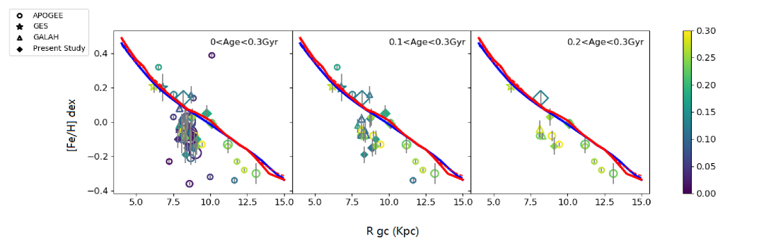
Figure 9: As in Fig 5, but colour coding the symbols by their age.The size of the symbols is proportional to the number of stars studied in the cluster to obtain the mean value reported here. (The open diamond represents ASCC 123 from Frasca et al. (2019)). The left panel shows all the clusters younger than 300Myr, while the middle and right panels show the fit without clusters younger than 100Myr and 200Myr, respectively. The fit to the models is quite reasonable when considering clusters older than 200Myr.

All these cases seem to indicate that we have to take the metallicity of young clusters with care. We also tried to understand which ages are more problematic. We show in Fig. 9 only clusters younger than 300 Myr, with the symbol size proportional to the number of stars available in each cluster. Apparently, the sample size is not the (main) source of the problem.

The clusters showing the larger discrepancy with respect to the model are younger than 200 Myr, and especially younger than 100 Myr. This is affecting analyses done both in the optical and the IR. As already discussed in literature (Yana Galarza et al., 2019; Baratella et al., 2020; Spina et al., 2020), in young dwarves chromospheric effects and considerable magnetic fields are at play, making a traditional 1-D LTE analysis based on minimising trends for Fe lines less than optimal. In fact, an intensification of strong absorption lines, those forming near the top of the stellar photosphere where the magnetic fields are more vigorous, has been observed as a function of the activity level during the stellar cycle (Yana Galarza et al., 2019; Spina et al., 2020). The cause of this effect can be imputed to Zeeman broadening of atomic lines or the effect of cool stellar spots. However, it is possible that many other phenomena related to the chromospheric activity, which are neglected in stellar models, are simultaneously at work contributing to this spectral variability. Interestingly, these problems for young stars have essentially only been studied and discussed in the case of MS or PMS stars. Our sample allow to shows clearly for the first time that the effect(s) extend also to giants. Indeed, this is not surprising, as the challenges posed by the modeling of atmospheres and spectra for giants are even more severe than those for dwarfs.

6 Summary

This paper provides the atmospherical parameters for 40 red giants/red clumps in 18 open clusters covering the Galactocentric distance range 7.7 ¡ R_gc ¡10 kpc. Almost all of them are young clusters, with 15 OCs between 40 and 600 Myr, two around 1.5 Gyr, and one (NGC 2682) at 4.2 Gyr. Their parameters were measured using very high-resolution, high S/N HARPS-N spectra, the EW method and 1D-LTE atmosphere models. The main results comprise:

(i) Very precise radial velocities with uncertainties of 0.05-0.25 km s^-1 were measured. The offset between our results and that from Gaia DR2 is -0.11$\pm$ 1.9 km s^-1.

(ii) Accurate stellar parameters were derived. For the stars located in the effective temperature range of 4200-5800 K uncertainties in $T_{\textrm{eff}}$ are around 60 K, and 0.12 dex in surface gravity. All of the clusters have metallicity close to solar, with a deviation within 0.05 dex.

(iii) We compared five of our clusters (Collinder 350, NGC 2682, Tombaugh 5, NGC 2548, Basel 11b) with results from previous work, finding no systematic bias in our determination. A few discrepant cases were examined.

(iv) We explored the trend between metallicities and Galactocentric distance combining our data with clusters from APOGEE, GES, OCCASO, GALAH, and other SPA OCs (ASCC 123, Gulliver 51, Ruprecht 171, NGC 2632, NGC 7044). We confirmed the variation of slope in the metallicity gradient near R_gc=14 kpc and found a gradient slope for the inner disc similar to other literature works.

(v) We used the combined sample to compare to the chemo-dynamical predictions by Minchev et al. (2014a), finding good agreement for clusters older than 0.3 Gyr. Conversely, younger clusters show a large dispersion, not predicted by models, with observed metallicities too low for the Galactocentric position (not explainable by radial mixing, given the young cluster age).

(vi) We examined the cases of young clusters with low metallicity, finding that some results may be doubtful. However, there seems to be a general difficulty in deriving accurate metallicities for clusters younger than about 200 Myr, both for dwarfs (confirming literature works) and giants. We tentatively ascribe this to the impropriety of the traditional analysis for young stars, as discussed in the previous section.

Table 7: Slope of the metallicity gradient from selected literature papers.

Reference	sample	d[Fe/H]/d Rgc	N OCs	Comment
Friel et al. (2002)	low-res optical spectra	-0.059$\pm 0.010$	39	7¡Rgc¡16 kpc, all agesa
Reddy et al. (2016)	high-res optical spectra	-0.052$\pm 0.011$	67	6¡Rgc¡12 kpc and $|z|<$500 pc
		-0.015$\pm 0.007$	12	12¡Rgc¿24 kpcb
Carrera et al. (2019)	APOGEE DR14, GALAH DR2	-0.052$\pm 0.003$	46	6¡Rgc¡13 kpcc
		-0.077$\pm 0.007$		6¡Rgc¡11kpcc
		0.018$\pm 0.009$		11¡Rgc¡13 kpcc
Casamiquela et al. (2019)	high-res optical spectra	-0.056$\pm 0.011$	18	Rgc¡12 kpc, all agesd
Donor et al. (2020)	APOGEE DR16	-0.068$\pm 0.004$	68	Rgc¡ 13.9 kpc, all agese
		-0.009$\pm 0.011$	3	Rgc¿13.9 kpc, all ages

Appendix A Data and results on individual stars

Table 8: Information on the observed targets based on Gaia DR2.

Name	Gaia ID	Ra	Dec	Gmag	BP-RP	Obs date	MJD-Obs	exp time
		(J2000)	(J2000)					(s)
ASCC 11	241730418805573760	03:32:04.87	+44:57:45.4	8.3675	1.507	2018-12-16	58468.84	1200
						2018-12-16	58468.82	1200
Alessi 1_1	402506369136008832	00:53:15.44	+49:31:53.8	9.824	1.187	2018-12-19	58471.82	1800
						2018-12-19	58471.84	1800
Alessi 1_2	402505991178890752	00:53:20.38	+49:28:49.7	9.808	1.176	2018-12-19	58471.87	1800
						2018-12-19	58471.89	1800
Alessi 1_3	402867593065772288	00:54:51.06	+49:53:17.2	9.565	1.186	2018-12-18	58470.86	1500
						2018-12-18	58470.88	1500
Alessi 1_4	402880684126058880	00:54:10.20	+49:40:08.9	7.099	1.349	2018-12-19	58471.93	1800
						2018-12-19	58471.95	1800
Alessi-Teusch 11	2184332753719499904	20:16:22.4	+52:06:18.4	7.099	1.349	2019-08-15	58710.86	690
Basel 11b_1	3424056131485038592	05:58:08.10	+21:57:44.7	10.989	1.782	2019-01-30	58513.90	3600
Basel 11b_2	3424055921028900736	05:58:10.12	+21:57:23.2	11.256	1.876	2019-01-30	58513.95	1800
						2019-01-30	58513.97	1800
						2019-01-30	58513.99	1800
Basel 11b_3	3424057540234289408	05:58:18.16	+21:58:43.7	11.320	1.884	2018-12-20	58472.19	1800
						2018-12-20	58472.21	1800
						2018-12-20	58472.24	1800
						2018-12-20	58472.26	1800
COIN-Gaia 30	532533682228608384	01:24:05.26	+70:25:25.1	8.352	1.762	2019-12-07	58824.85	1400
Collinder 463_1	534207555539397888	01:33:49.45	+71:51:09.6	7.946	1.632	2018-12-19	58471.80	1200
Collinder 463_2	534363067715447680	01:45:09.15	+71:53:25.3	7.725	1.572	2018-12-17	58469.81	1200
Gulliver 18	1836389309820904064	20:11:43.9	26:35:07.0	8.964	2.178	2019-08-10	58705.88	1380
Gulliver 24	430035249779499264	00:04:28.47	+62:42:04.4	10.494	1.927	2019-08-12	58707.15	1500
						2019-08-12	58707.16	1500
Gulliver 37	2024469226291472000	19:28:18.44	+25:22:53.4	10.592	1.559	2019-08-13	58708.94	608
						2019-08-13	58708.93	1500
NGC 2437_1	3029609393042459392	07:41:36.9	-14:26:11.2	10.277	1.338	2018-12-17	58469.08	1800
						2018-12-17	58469.10	1800
NGC 2437_2	3029202711180744832	07:41:28.52	-14:54:17.5	10.293	1.285	2018-12-17	58469.12	1800
						2018-12-17	58469.15	1800
NGC 2437_3	3030364134752459904	07:41:00.64	-14:12:08.4	10.417	1.274	2018-12-17	58469.17	1800
						2018-12-17	58469.19	1800
NGC 2437_4	3029132686034894592	07:42:47.85	-15:17:44.16	10.838	1.302	2018-12-18	58470.18	2400
						2018-12-18	58470.20	2400
NGC 2437_5	3029156222454419072	07:42:41.24	-14:59:51.4	10.948	1.262	2018-12-19	58471.17	2400
						2018-12-19	58471.20	2400
NGC 2437_6	3029207006148017664	07:41:19.42	-14:48:47.5	9.877	1.332	2018-12-18	58470.10	1500
						2018-12-18	58470.12	1500
NGC 2437_7	3029226694277998080	07:41:19.36	-14:40:59.7	9.975	1.322	2018-12-08	58470.14	1500
						2018-12-08	58470.16	1500
NGC 2509	5714209934411718784	08:00:44.36	-19:06:59.4	12.883	1.275	2019-01-15	58498.07	2400
						2019-01-15	58498.10	2400
						2019-01-15	58498.13	2400
NGC 2548_1	3064481400744808704	08:13:35.42	-05:53:02.04	9.377	1.098	2018-12-17	58469.24	1200
						2018-12-17	58469.25	1200
NGC 2548_2	3064537647636773760	08:12:37.24	-05:40:51.0	9.151	1.111	2018-12-18	58470.24	1200
						2018-12-18	58470.25	1200
NGC 2548_3	3064579703955646976	08:14:28.10	-05:42:16.09	9.187	1.190	2018-12-19	58471.23	1200
						2018-12-19	58471.25	1200
NGC 2548_4	3064486692144030336	08:13:40.44	-05:46:24.96	8.873	0.786	2018-12-17	58469.27	1800
NGC 7082_1	1972288740859811072	21:28:48.97	+47:06:54.2	8.171	1.508	2019-12-08	58825.80	1400
NGC 7082_2	1972288637780285312	21:28:34.58	+47:05:22.92	7.622	1.470	2019-12-07	58824.81	1400
NGC 7209_1	1975004019170020736	22:05:09.94	+46:31:25.3	9.766	1.323	2019-08-14	58709.14	1725
						2019-08-14	58709.16	1725
NGC 7209_2	1975002919658397568	22:05:17.63	+46:29:00.6	8.891	1.734	2019-08-14	58709.12	2070
Tombaugh 5_1	473266779976916480	03:47:30.99	+59:02:50.8	11.163	2.123	2018-12-20	58472.11	1800
						2018-12-20	58472.09	1800
						2018-12-20	58472.15	1800
						2018-12-20	58472.13	1800
Tombaugh 5_2	473275782228263296	03:48:32.98	+59:15:16.56	11.366	2.147	2019-01-15	58497.06	1800
						2019-01-14	58497.04	1800
						2019-01-15	58498.00	1800
Tombaugh 5_3	473268424940932864	03:47:46.78	+59:05:36.6	11.138	2.028	2019-01-14	58498.03	1800
						2019-01-14	58497.98	1800
						2019-01-14	58497.02	1800
UPK 219	2209440823287736064	23:30:29.72	+65:08:35.3	8.728	1.734	2019-12-08	58825.84	1400
Comparison clusters
Collinder 350_1	4372743213795720704	17:46:24.88	+01:02:39.7	5.957	1.869	2018-08-20	58350.87	300
						2018-08-20	58350.88	300
Collinder 350_2	4372572888274176768	17:48:43.82	+01:09:51.1	8.421	1.485	2018-08-20	58350.88	1380
NGC 2682_1	604921512005266048	08:51:26.17	+11:53:51.9	10.202	1.238	2020-02-02	58881.07	1500
						2020-02-02	58881.08	1500
NGC 2682_2	604920202039656064	08:51:59.51	+11:55:04.8	10.205	1.243	2020-02-02	58881.10	1500
						2020-02-02	58881.12	1500
NGC 2682_3	604904950611554432	08:51:50.19	+11:46:06.9	10.511	1.110	2020-02-02	58881.14	1500
						2020-02-02	58881.16	1500
						2019-12-08	58825.19	1500
						2019-12-08	58825.21	1500
						2019-12-08	58825.22	1500
						2020-03-11	58919.04	1500
						2020-03-11	58919.06	1500
NGC 2682_4	604917728138508160	08:51:23.76	+11:49:49.3	11.231	1.073	2020-03-10	58918.99	1420
						2020-03-11	58919.00	1420
						2020-03-11	58919.02	1420

Table 9: Final atmospheric parameters of observed targets

Name	Gaia ID	$T_{\textrm{eff}}$	$\sigma$ $T_{\textrm{eff}}$	$\log$ g	$\sigma$	[Fe/H]	$\sigma_{1}$	$\sigma_{2}$	$\log\epsilon$	std	Nlines	$\log\epsilon$	std	Nlines	vmicro	$\sigma$
		(K)		(dex)	$\log$ g	(dex)	[Fe/H]	[Fe/H]	Fe I		Fe I	Fe II		Fe II	(km s-1)	vmicro
ASCC 11	241730418805573760	5250	70	2.15	0.10	-0.14	0.05	0.06	7.360	0.159	46	7.360	0.210	10	2.4	0.3
Alessi 1_1	402506369136008832	5000	70	2.65	0.15	-0.10	0.05	0.05	7.392	0.181	74	7.391	0.136	16	1.5	0.1
Alessi 1_2	402505991178890752	5200	70	3.20	0.10	0.08	0.10	0.10	7.583	0.135	75	7.587	0.128	15	1.5	0.2
Alessi 1_3	402867593065772288	5250	65	3.27	0.10	0.07	0.06	0.06	7.576	0.105	75	7.575	0.098	15	1.6	0.1
Alessi 1_4	402880684126058880	5120	60	3.09	0.06	-0.05	0.10	0.10	7.470	0.122	72	7.476	0.089	16	1.6	0.1
Alessi-Teusch 11	2184332753719499904	4560	50	2.10	0.15	-0.19	0.05	0.05	7.310	0.172	75	7.311	0.219	16	2.1	0.2
Basel 11b_1	3424056131485038592	5180	50	3.15	0.13	0.00	0.05	0.05	7.500	0.093	68	7.507	0.127	13	2.2	0.1
Basel 11b_2	3424055921028900736	5220	30	3.07	0.10	0.02	0.03	0.03	7.525	0.141	72	7.529	0.135	15	2.2	0.2
Basel 11b_3	3424057540234289408	4950	50	2.83	0.10	-0.04	0.05	0.05	7.464	0.136	77	7.467	0.116	15	2.1	0.1
COIN-Gaia 30	532533682228608384	5200	50	3.40	0.05	0.03	0.05	0.05	7.538	0.158	71	7.552	0.163	15	2.3	0.2
Collinder 463_1	534207555539397888	4730	30	2.12	0.10	-0.20	0.05	0.05	7.310	0.130	72	7.310	0.180	16	2.5	0.1
Collinder 463_2	534363067715447680	4730	30	2.30	0.15	-0.10	0.05	0.05	7.410	0.131	70	7.410	0.207	16	2.4	0.1
Gulliver 18	1836389309820904064	4590	100	2.60	0.17	-0.10	0.04	0.05	7.409	0.212	76	7.395	0.281	16	2.8	0.3
Gulliver 24	430035249779499264	4450	50	2.50	0.15	-0.18	0.03	0.03	7.317	0.145	74	7.316	0.240	16	2.0	0.2
Gulliver 37	2024469226291472000	4850	50	3.65	0.12	0.10	0.03	0.04	7.602	0.213	62	7.604	0.403	10	0.8	0.6
NGC 2437_1	3029609393042459392	5050	50	2.77	0.12	0.04	0.05	0.05	7.546	0.142	64	7.548	0.109	12	2.1	0.1
NGC 2437_2	3029202711180744832	5250	75	3.32	0.10	0.07	0.05	0.05	7.572	0.140	62	7.578	0.171	13	2.2	0.2
NGC 2437_3	3030364134752459904	5300	110	3.13	0.10	-0.05	0.05	0.05	7.450	0.176	62	7.447	0.149	13	2.3	0.2
NGC 2437_4	3029132686034894592	5085	65	2.90	0.10	0.00	0.05	0.05	7.508	0.111	62	7.498	0.089	15	1.7	0.1
NGC 2437_5	3029156222454419072	5030	75	2.85	0.15	0.00	0.10	0.10	7.503	0.163	74	7.505	0.161	16	1.7	0.1
NGC 2437_6	3029207006148017664	4990	65	2.72	0.10	0.00	0.05	0.06	7.443	0.238	72	7.444	0.266	15	2.1	0.1
NGC 2437_7	3029226694277998080	4650	90	2.27	0.20	-0.07	0.08	0.08	7.440	0.216	73	7.440	0.272	16	1.2	0.1
NGC 2509	5714209934411718784	4705	40	2.53	0.20	-0.10	0.05	0.06	7.394	0.213	72	7.392	0.330	16	1.5	0.3
NGC 2548_1	3064481400744808704	5370	70	3.67	0.15	0.00	0.05	0.05	7.507	0.131	60	7.504	0.155	15	2.0	0.2
NGC 2548_2	3064537647636773760	5050	50	2.65	0.10	-0.02	0.04	0.04	7.479	0.068	62	7.480	0.101	15	1.6	0.1
NGC 2548_3	3064579703955646976	4930	50	2.70	0.10	-0.01	0.05	0.05	7.490	0.079	61	7.491	0.083	13	1.6	0.1
NGC 2548_4	3064486692144030336	5200	50	3.18	0.10	-0.07	0.07	0.07	7.434	0.110	62	7.439	0.142	14	0.4	0.1
NGC 7082	1972288740859811072	4994	50	2.25	0.1	-0.15	0.05	0.07	7.360	0.144	63	7.361	0.199	12	3.0	0.2
NGC 7209_1	1975004019170020736	4880	50	2.35	0.15	0.00	0.03	0.07	7.439	0.110	74	7.433	0.155	16	1.7	0.2
NGC 7209_2	1975002919658397568	4600	30	2.79	0.15	-0.07	0.05	0.05	7.433	0.136	67	7.435	0.316	16	2.5	0.2
Tombaugh 5_1	473266779976916480	5010	50	3.17	0.15	0.04	0.05	0.05	7.543	0.166	72	7.546	0.185	15	2.2	0.1
Tombaugh 5_2	473275782228263296	4900	50	2.31	0.1	-0.07	0.05	0.01	7.438	0.080	74	7.436	0.073	14	2.0	0.2
Tombaugh 5_3	473266779976916480	5150	50	3.08	0.15	0.07	0.05	0.05	7.570	0.095	69	7.576	0.147	15	2.2	0.2
UPK 219	2209440823287736064	5203	150	3.01	0.10	0.02	0.05	0.05	7.528	0.166	74	7.530	0.283	16	2.7	0.2
Collinder 350_1	4372743213795720704	4200	50	1.30	0.20	-0.40	0.08	0.08	7.120	0.149	71	7.130	0.256	16	2.2	0.1
Collinder 350_2	4372572888274176768	5300	50	3.15	0.1	0.02	0.05	0.05	7.521	0.079	71	7.526	0.095	15	1.6	0.1
NGC 2682_1	604921512005266048	4687	50	2.37	0.07	-0.05	0.05	0.05	7.454	0.174	75	7.453	0.181	16	1.5	0.2
NGC 2682_2	604920202039656064	4900	110	2.76	0.1	0.02	0.05	0.05	7.520	0.132	69	7.528	0.168	15	1.7	0.2
NGC 2682_3	604904950611554432	5000	50	2.77	0.1	-0.03	0.03	0.03	7.467	0.096	67	7.467	0.082	14	1.2	0.2
NGC 2682_4	604917728138508160	5195	50	3.25	0.10	0.00	0.05	0.03	7.501	0.108	67	7.502	0.164	14	1.3	0.2
SUN		5770	40	4.44	0.08	-0.03	0.03	0.03	7.477	0.077	76	7.477	0.083	16	1.0	0.1