On Soliton Resolution for a Lattice

Abstract.

The soliton resolution conjecture for evolution PDEs of dispersive type states (vaguely) that generic initial data of finite energy give rise asymptotically to a set of receding solitons and a decaying background radiation.

In this letter, we investigate a possible extension of this conjecture to discrete lattices of the Fermi-Pasta-Ulam-Tsingou type (rather than PDEs) in two cases; the case with initial data of finite energy and a more general case with initial data that are a short range perturbation of a periodic function.

In the second case, inspired by rigorous results on the Toda lattice, we suggest that the soliton resolution phenomenon is replaced by something somewhat more complicated: a short range perturbation of a periodic function actually gives rise to different phenomena in different regions. Apart from regions of (asymptotically) pure periodicity and regions of solitons in a periodic background, we also observe “modulated” regions of fast oscillations with slowly varying parameters like amplitude and phase.

We have conducted some numerical calculations to investigate if this trichotomy (pure periodicity + solitons + modulated) persists for any discrete lattices of the Fermi-Pasta-Ulam-Tsingou type. For small perturbations of integrable lattices like the linear harmonic lattice, the Langmuir chain and the Toda lattice, this is true. But in general even chaotic phenomena can occur.

1. Historical Introduction and a Statement of the Soliton Resolution Conjecture in a Periodic Background

A classical observation going back to the seminal discovery of Zabusky and Kruskal ([17]) states that a local (or short range) perturbation of the trivial stationary solution of a completely integrable soliton PDE (like KdV or NLS) or lattice (like Toda), eventually splits into a number of receeding solitons plus a (uniformly) decaying background radiation. The first complete description for the long time asymptotics of the KdV equation were given in [1]. Rigorous proofs can be constructed for any system solvable via the inverse scattering theory. Such proofs routinely employ the asymptotic analysis of the associated Riemann-Hilbert factorisation problems, at least in the case of one space dimension ([4], [6], [8], [9]), where the inverse scattering problem is equivalent to a Riemann-Hilbert factorisation problem in the complex plane.

More recently, an even more daring conjecture has begun to take shape ([15], [2]): for $any$ dispersive PDE of NLS or KdV type in any spatial dimension (!), generic initial data of bounded energy give rise asymptotically to a set of receeding solitons and a decaying background radiation.

Our aim here is to investigate the Soliton Resolution Conjecture for one-dimensional, constant or periodic background, uniform (without impurities, i.e. all particles are of the same mass $m=1$), doubly infinite lattices with nearest neighbor interaction (each particle only affects its two neighbors, one on the left and one on the right).

To be precise, let $x_{n}(t)=x(n,t)$, $(n,t)\in{\mathbb{Z}}\times{\mathbb{R}}$ denote the displacement (from its equilibrium) of the $n^{th}$ particle in the chain at time $t$. If we denote by $V(x_{n+1}-x_{n})$, $n\in\mathbb{Z}$ the interaction potential between neighboring particles, then the equation of motion is given by

(1.1) $$\frac{d^{2}x_{n}}{dt^{2}}=V^{\prime}(x_{n+1}-x_{n})-V^{\prime}(x_{n}-x_{n-1}),\quad(n,t)\in{\mathbb{Z}}\times{\mathbb{R}}$$

where $V^{\prime}(x)=\frac{dV}{dx}(x)=:-F(x)$, $V$ being the potential function and $F$ the corresponding force. What can we say about the long time asymptotics of this system given some general conditions on the behaviour of the initial data $x_{n}$, and $dx_{n}/dt$ at time $t=0$ and as $n\to\pm\infty$?

Let us begin by presenting a Soliton Resolution Conjecture in a constant background. To be more precise, we assume that $x_{n}$, and $dx_{n}/dt$ tend to $0$ fast enough as $n\to\pm\infty$ (at time $0$). (See (A.3)n the Appendix A, for a definition of ”fast enough” in the case of the Toda lattice, where rigorous results exist. Even somewhat weaker definitons are probably sufficent.) The claim is that the solution is asymptotically given by a sum of solitary waves with different speeds plus a small ”radiation” term that decays in time.

The first rigorous study of this phenomenon in a constant background was done in [8] for the special case of the Toda lattice, with $V(x)=e^{-x}+x$, in the case where the associated Jacobi operatorm has no eigenvalues. Eigenvalues were added later in [13]. In these works it was shown that the error term is actually of order $O(t^{-1/2})$ uniformly in $n$, at least away from the two regions where $n/t$ is $\pm 1+o(1)$. With some more work, one can actually show that in these small regions the error order is $O(t^{-1/3})$.

The first rigorous study of the analogous phenomenon in a periodic background was done in [10], also for the Toda lattice, where numerical experiments were presented and complete analytic formulas where given for the asymptotics of the doubly infinite periodic Toda lattice under a ”short range” perturbation (again see appendices A and B for the exact condition on the initial data and the exact asymptotic formulae). The proofs were presented in [11] in the case where the associated Lax operator (tridiagonal Jacobi operator in this case) has no eigenvalues. Again, one uses asymptotic analysis of the associated Riemann-Hilbert holomorphic factorisation problems, with the extra novelty that such problems are posed on a Riemann surface. Once this analysis was achieved, eigenvalues were easily added ([12]) and higher order asymptotics have also been presented ([11]).

Figure 1 exemplifies the general situation in the periodic background case. As time goes to infinity, the (n,t) space is divided into several regions. There are three kinds of such regions: there are regions of periodicity (the period being equal to the period of the unpertrubed lattice), there are solitons in a periodic background, and then there are regions where the lattice undergoes modulated oscillations with a large (order $1/t$) frequency and slowly varying (with $n/t$) amplitude and phase. Phenomena appear in two different scales and are naturally expressed in two new variables: the fast one being $1/t$ and the slow one being $n/t$. The regions of periodicity and the modulation regions are open cones bounded by half-lines (if we consider only positive times t) emerging at the origin. The soliton regions are small (in $1/t$) regions around (some of) these half-lines. The slopes of the half-lines are the speeds of the solitons.

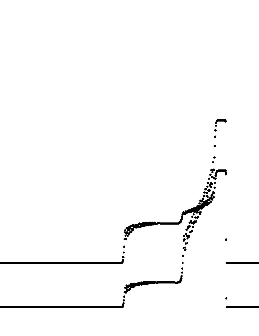
(a) $t=250$

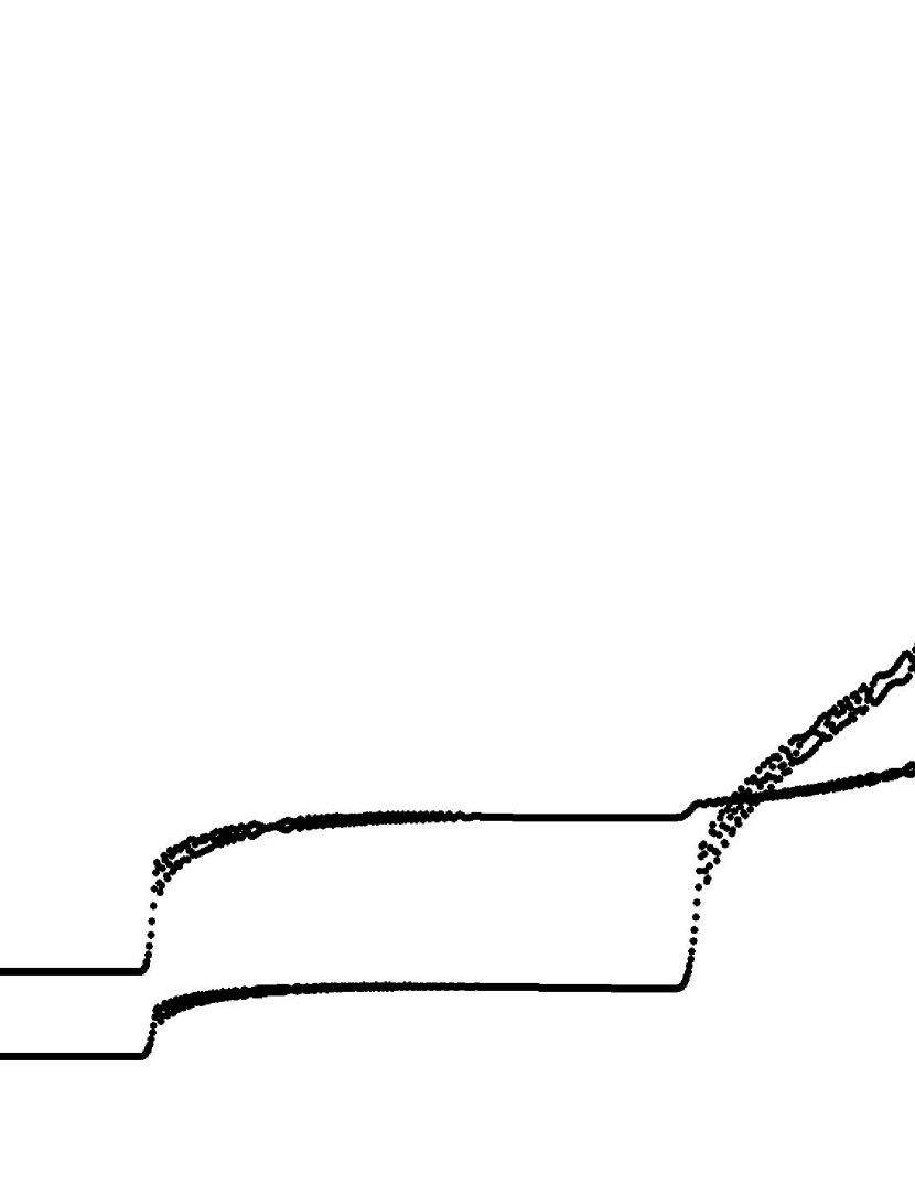
(b) $t=700$

Figure 1. Two snapshots at times $t=250$ (A) and $t=700$ (B) of the (numerically computed) solution of a Toda lattice, with a period 2 initial condition.

In each figure in Figure 1, the two observed lines express the variables $x_{n}(t)$ as functions of the particle index $n$ at a frozen time $t$. In some areas, the lines seem to be continuous. This is due to the fact that we have plotted a huge number of particles (2048 particles) and also due to the 2-periodicity in space. So, one can think of the two lines as the even- and odd-numbered particles of the lattice.

We first note the single soliton which separates two regions of apparent periodicity on the right. On soliton’s left side, we observe three different areas with apparently periodic solutions of period two. Finally, there are some transitional (modulation) regions which interpolate between the different period two regions.

A natural question is whether this behaviour is ubiquitous in any FPUT lattice. Namely, that the $(n,t)$ half-plane is divided by half-lines into pure periodic and modulated regions as above, while sometimes solitons appear in the boundaries of such regions.

Standard KAM theory suggests that this might happen only for small pertrubations while in general chaos can occur. On the other hand our situation here is somewhat different to standard KAM problems in that we have non-periodic perturbations of a periodic lattice so the short range perturbations have more space to travel into.

2. Simulations’ Setup

As mentioned in the first paragraph, we are dealing with one-dimensional, periodic, uniform, doubly infinite lattices with nearest neighbor interaction. So for our numerics, we will consider the ODE system (1.1) with $(n,t)\in\{1,2,\dots,N\}\times{\mathbb{R}}$ for fixed $N\in\mathbb{N}$ and impose the periodic condition $x_{N+1}=x_{1}$. Defining $q_{n}:=x_{n}$ and $p_{n}:=\dot{q}_{n}=\dot{x}_{n}=\frac{dx_{n}}{dt}$, system (1.1) can be written as

(2.1) $$\begin{cases}\dot{q}_{n}=p_{n}\\ \dot{p}_{n}=V^{\prime}(q_{n+1}-q_{n})-V^{\prime}(q_{n}-q_{n-1}),\quad(n,t)\in\{1,2,\dots,N\}\times{\mathbb{R}}\end{cases}$$

with Hamiltonian

(2.2) $$\mathcal{H}(\mathbf{q},\mathbf{p})=\sum_{n=1}^{N}\Bigg{[}\frac{1}{2}p_{n}^{2}+V(q_{n+1}-q_{n})\Bigg{]}$$

where $\mathbf{q}=(q_{1},q_{2},\dots,q_{N})$ and $\mathbf{p}=(p_{1},p_{2},\dots,p_{N})$. As far as the initial conditions are concerned, we either require

• perturbed zero (or trivial) background conditions, specifically

  (2.3) $$\begin{cases}q_{n}(0)=exp\{-\big{(}\frac{n-\frac{N}{4}}{4}\big{)}^{2}\}\\ p_{n}(0)=0\end{cases},n=1,2,\dots,N\quad\text{or}$$

• perturbed periodic background conditions (the period being $2$), i.e.

  (2.4) $$\begin{cases}q_{n}(0)=0\\ p_{n}(0)=(-1)^{n}+2\delta_{n}^{N/2}\end{cases},n=1,2,\dots,N$$

  where $\delta_{i}^{j}$ denotes Kronecker’s delta.

Our simulations are based on MATLAB^® in which we consider $N=2048$ and use $ode45$ as an integration method. For the time discretization we use a time-step size of $1$ for a total number of $800$ steps. The algorithm (see appendix C) is similar to that found in Scholarpedia’s article about the FPUT nonlinear lattice oscillations which in fact comes from [3]. Finally, for the potential function $V$ we consider the following candidates

• FPUT potential $V(x)=\frac{1}{2}x^{2}+\frac{\alpha}{3}x^{3}+\frac{\beta}{4}x^{4}$, where $\alpha,\beta$ are real parameters. More presicely we only consider its two offsprings, the FPUT$-\alpha$ potential (for $\beta=0$) $V(x)=\frac{1}{2}x^{2}+\frac{\alpha}{3}x^{3}$ and the FPUT$-\beta$ potential (for $\alpha=0$) $V(x)=\frac{1}{2}x^{2}+\frac{\beta}{4}x^{4}$

• harmonic potential $V(x)=\frac{1}{2}x^{2}$

• Hertz potential $V(x)=\begin{cases}c|x|^{5/2},\quad x<0\\ 0,\quad x\geq 0\end{cases}$, where $c$ is a real parameter

• Langmuir (or Volterra or Kac-van Moerbeke or Moser or discrete KdV) potential $V(x)=e^{x}$

• perturbed Langmuir potential $V(x)=e^{x}+\alpha x^{3}+\beta x^{4}$, where $\alpha,\beta$ are real parameters. We study the cases $V(x)=e^{x}+\alpha x^{3}$ and $V(x)=e^{x}+\beta x^{4}$ separately.

• $(2,1)$Lennard-Jones potential $V(x)=\varepsilon\bigg{[}\Big{(}\frac{d}{d+x}\Big{)}^{2}-2\frac{d}{d+x}+1\bigg{]}$, where $\varepsilon,d$ are real parameters

• Morse potential $V(x)=\gamma(e^{-\delta x}-1)^{2}$, where $\gamma,\delta$ are real parameters

• Toda potential $V(x)=e^{-x}+x$

• perturbed Toda potential $V(x)=e^{-x}+x+\alpha x^{3}+\beta x^{4}$, where $\alpha,\beta$ are real parameters. We study the cases $V(x)=e^{-x}+x+\alpha x^{3}$ and $V(x)=e^{-x}+x+\beta x^{4}$ separately.

Closing this paragraph, it is essential to add that all of our numerics have been checked for accuracy in the sense that the quantities (e.g. total momentum, hamiltonian) that are expected to be conserved are indeed (almost) conserved. We observed only very small deviations from these constant values.

3. Numerical results with trivial background

In this section we present some numerical experiments which support the soliton resolution conjecture in the case of a lattice with trivial background. Here, and in the next section, we plot $q_{n}$ as a function of $n$ at two specific times. Again, $n$ is a discrete variable, but our pictures cover around 1800 particles (excluding 124 from each side of the altogether 2048 particle chain), so what should be a discrete sequence of dots may look like a smooth curve. If we zoomed in, we should be able to distinguish the dots. Again, in the integrable cases (i.e. Langmuir and Toda), the result can be proved ([14], [8], [13]) with the help of the inverse scattering theory.

Our first numerical simulation is concerned with the FPUT lattice. More specifically with FPUT$-\alpha$ potential. We have completed experiments with different values of the $\alpha$ parameter. We put $\alpha=0.425$, $0.4$, $0.25$, $0.1$ and $0.01$. All results turned out to be qualitively the same. Figure 2 shows these results in the case of an FPUT-$\alpha$ potential with $\alpha=0.25$.

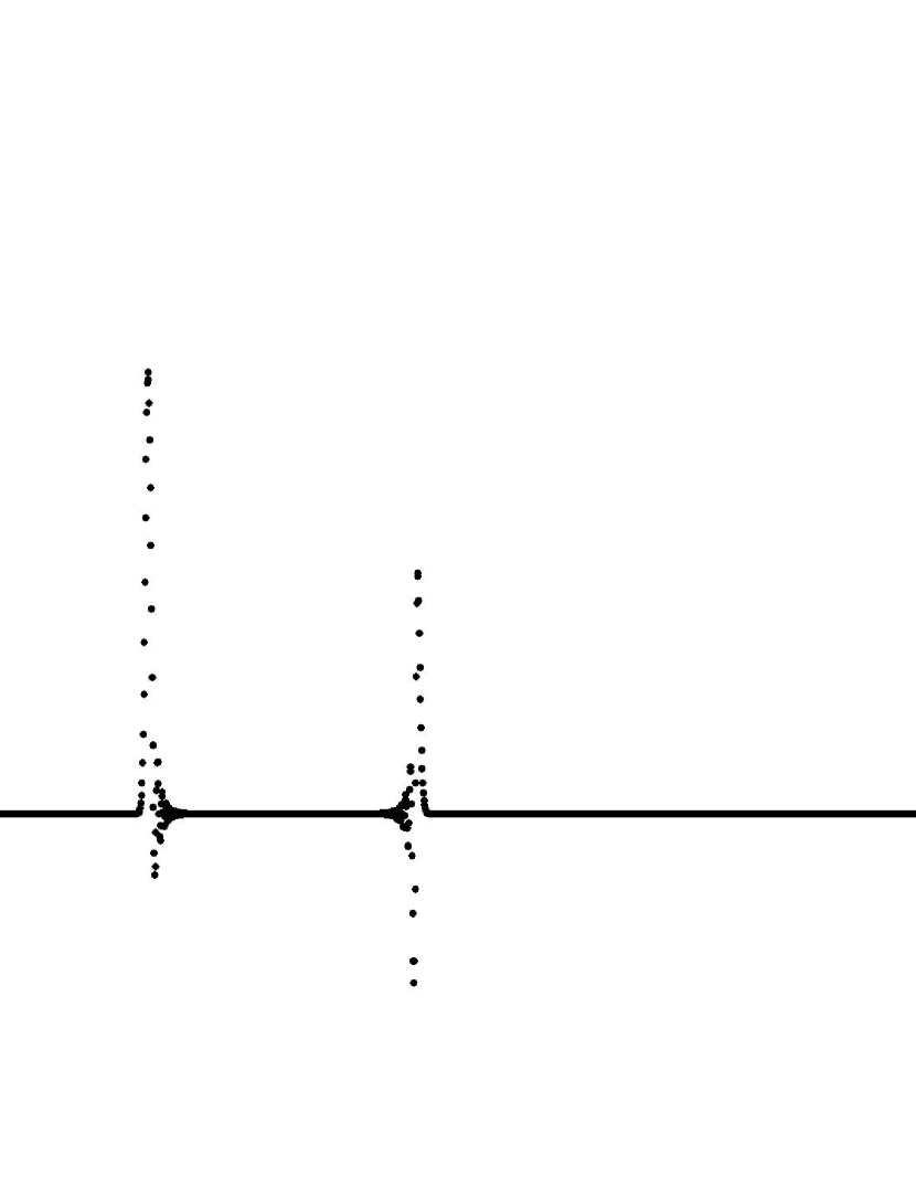
(a) $t=225$

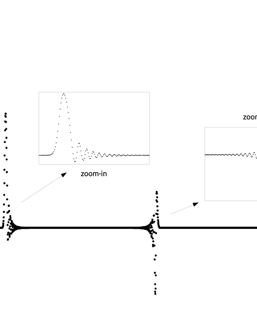
(b) $t=450$

Figure 2. Two snapshots at times $t=225$ (A) and $t=450$ (B) of the (numerically computed) solution of a FPUT$-\alpha$ lattice for $\alpha=0.25$ with zero background initial condition.

Next, we experimented with the FPUT-$\beta$ potential. As before, we tried $\alpha=0.425$, $0.4$, $0.25$, $0.1$ and $0.01$. Once more, all the outcomes had the same qualitative nature. In Figure 3 we present the results of our numerics for the FPUT-$\beta$ potential with $\beta=0.01$.

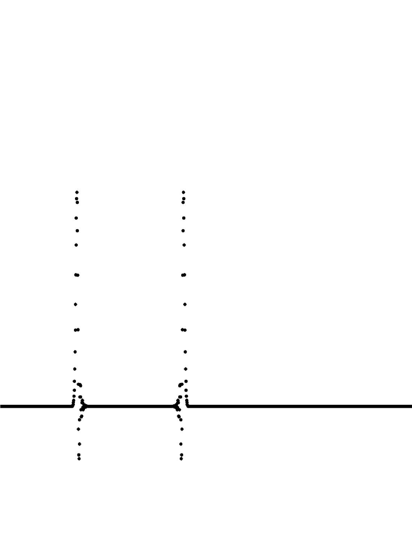
(a) $t=200$

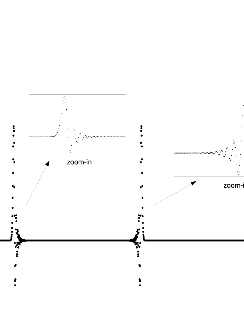
(b) $t=400$

Figure 3. Two snapshots at times $t=200$ (A) and $t=400$ (B) of the (numerically computed) solution of a FPUT$-\beta$ lattice for $\beta=0.01$ with zero background initial condition.

In both cases the soliton resolution is crystal clear! We observe two well-defined solitons with constant amplitude and shape and well defined constant speeds. The background radiation is very small. We have conducted many more simulations for the case of zero background. Following is a list of the potentials that gave similar results (identical pictures with the figures above)

• harmonic

• Langmuir

• small perturbations (e.g. $\alpha,\beta=0.01$ or less) of the Langmuir

• $(2,1)-$Lennard-Jones for big values of the parameter $d$ representing lattice spacing (in equilibrium), e.g. $d=10$ or larger. In this case, $\varepsilon$ can be anything

• Morse for small values of the parameter $\delta$. $\gamma$ takes arbitrary values.

• Toda

• small perturbations (e.g. $\alpha,\beta=0.1$ or less) of Toda

On the other hand, other experiments give something different! The following pictures show a representative sample of them.

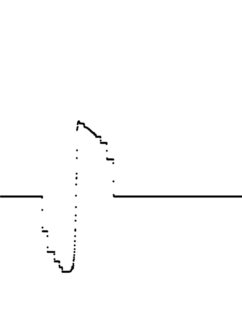
(a) $t=250$

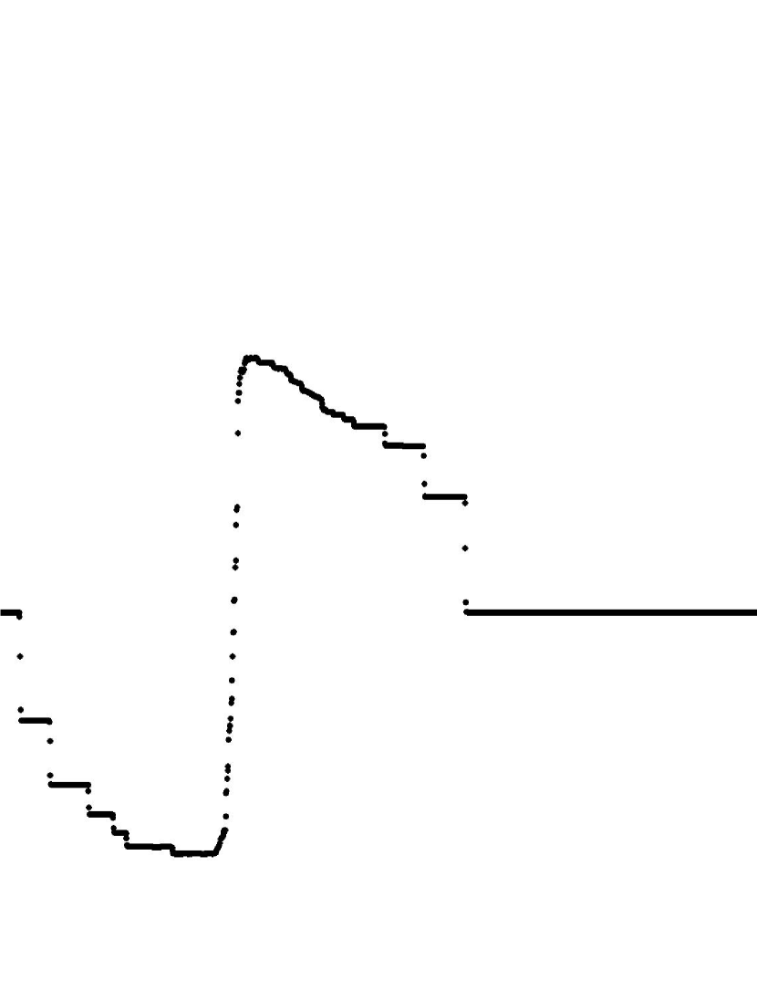
(b) $t=500$

Figure 4. Two snapshots at times $t=250$ (A) and $t=500$ (B) of the (numerically computed) solution of a Hertz lattice for $c=1$ with zero background initial condition.

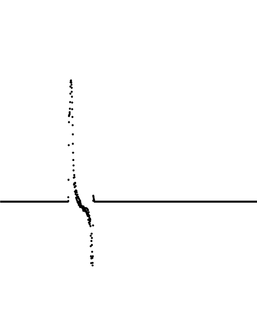
(a) $t=200$

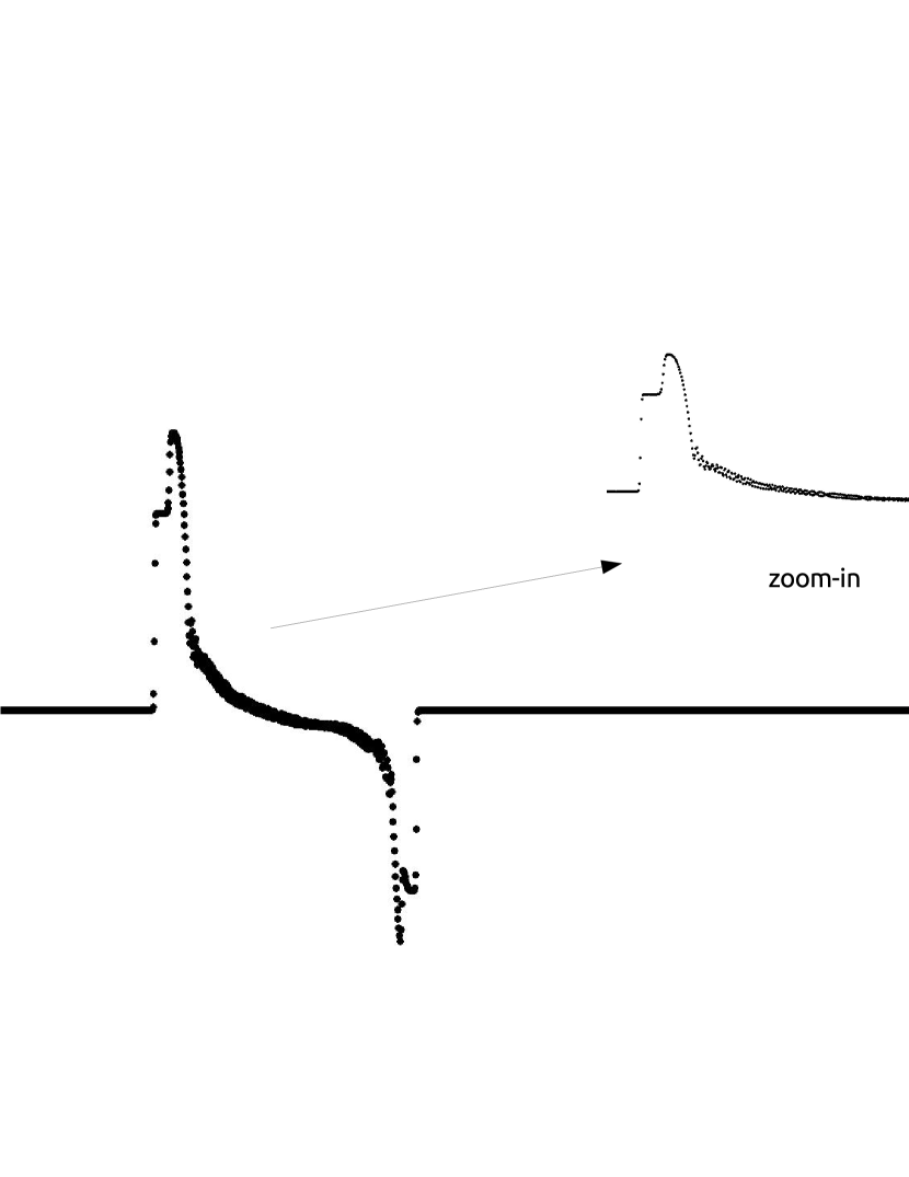
(b) $t=600$

Figure 5. Two snapshots at times $t=200$ (A) and $t=600$ (B) of the (numerically computed) solution of a Langmuir lattice with a cubic perturbation of $\alpha=0.1$ with zero background initial condition.

Below, in Figure 6 we see the results coming from the integrator for a $(2,1)-$Lennard-Jones lattice for $d=1$ and $\varepsilon=10$ with zero background initial condition. Qualitatively, we get the same result for a Morse potential with $\gamma=1/2$ and $\delta=1$.

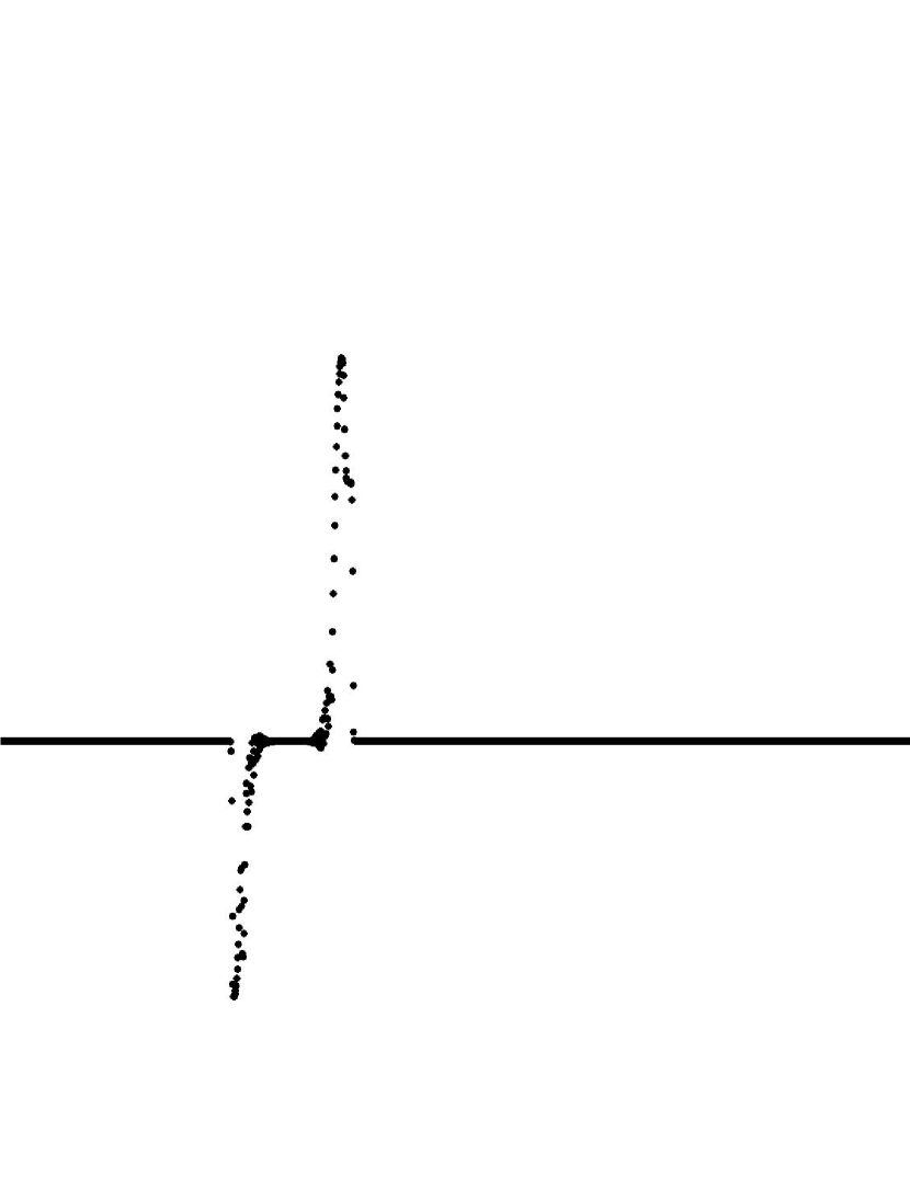
(a) $t=20$

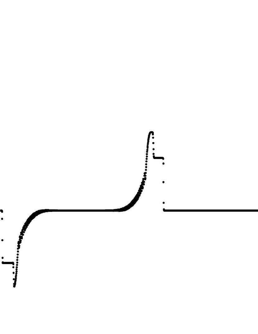
(b) $t=90$

Figure 6. Two snapshots at times $t=20$ (A) and $t=90$ (B) of the (numerically computed) solution of a $(2,1)-$Lennard-Jones lattice for $d=1$ and $\varepsilon=10$ with zero background initial condition.

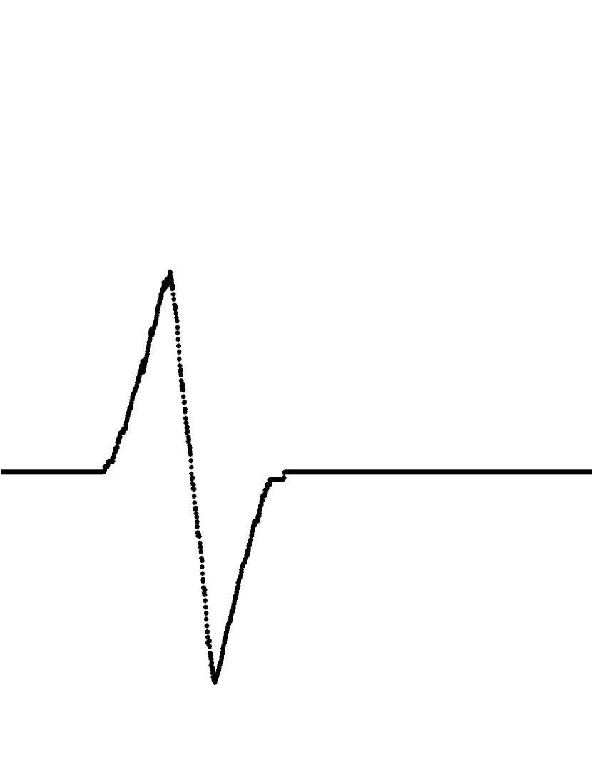
(a) $t=25$

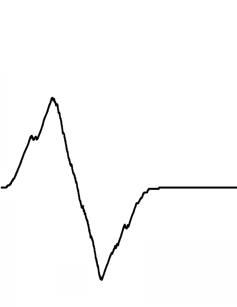
(b) $t=50$

Figure 7. Two snapshots at times $t=25$ (A) and $t=50$ (B) of the (numerically computed) solution of a Toda lattice with a cubic perturbation of $\alpha=10$ and zero background initial condition.

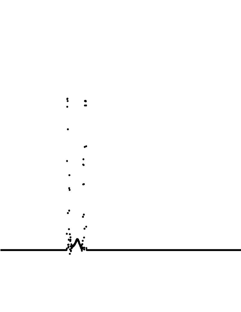
(a) $t=25$

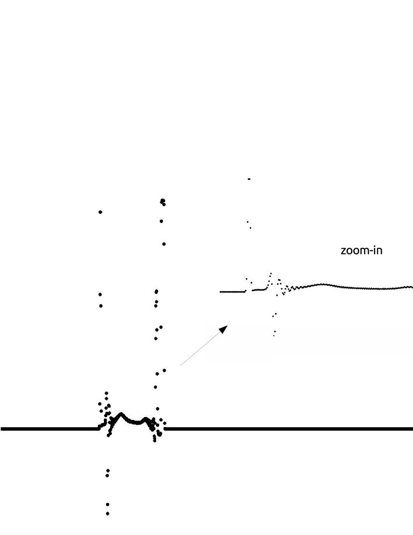
(b) $t=50$

Figure 8. Two snapshots at times $t=25$ (A) and $t=50$ (B) of the (numerically computed) solution of a Toda lattice with a quartic perturbation of $\beta=10$ and zero background initial condition.

4. Numerical results with periodic background

In this section we present some numerical experiments which support our amended soliton resolution conjecture in the case of a lattice with nearest neighbour interaction but in this case for a periodic background. In the case of the harmonic lattice, one has the following findings

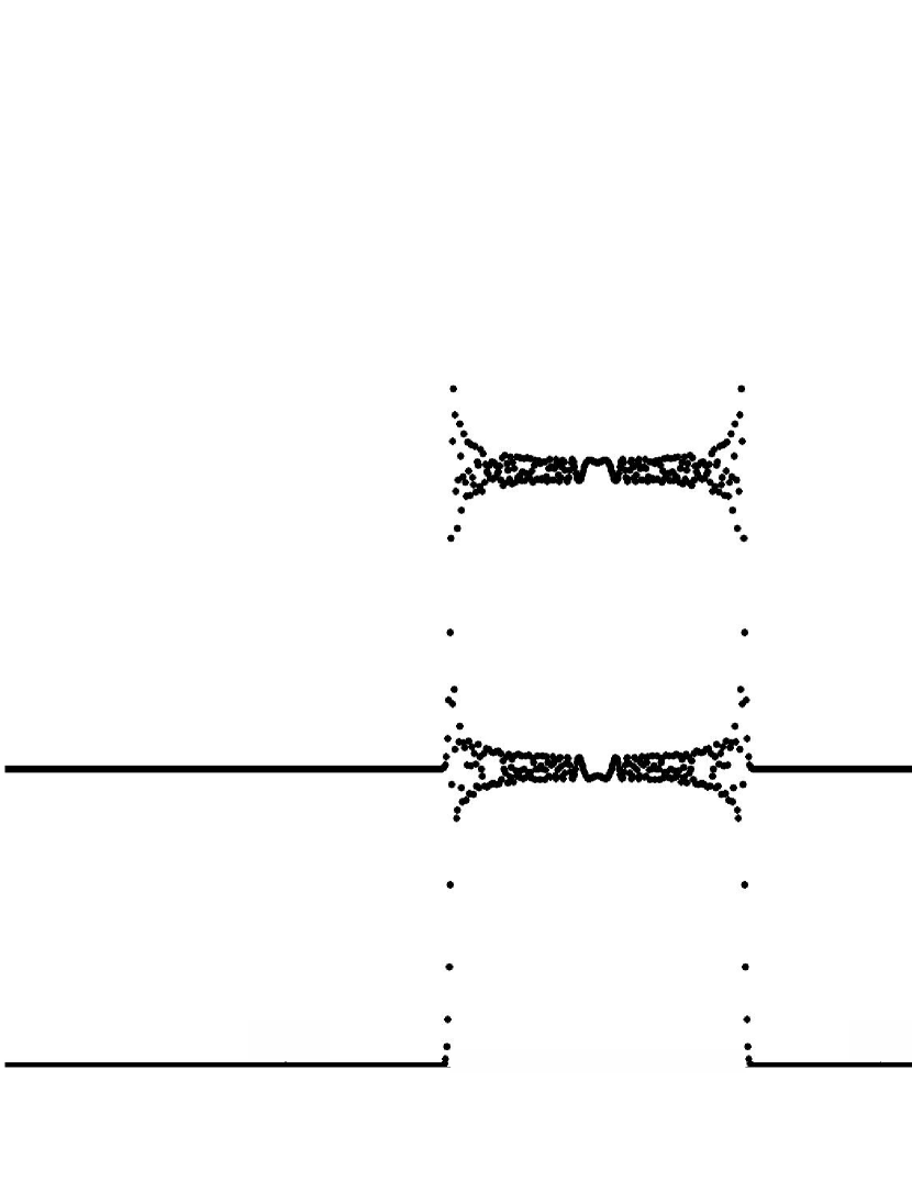
(a) $t=250$

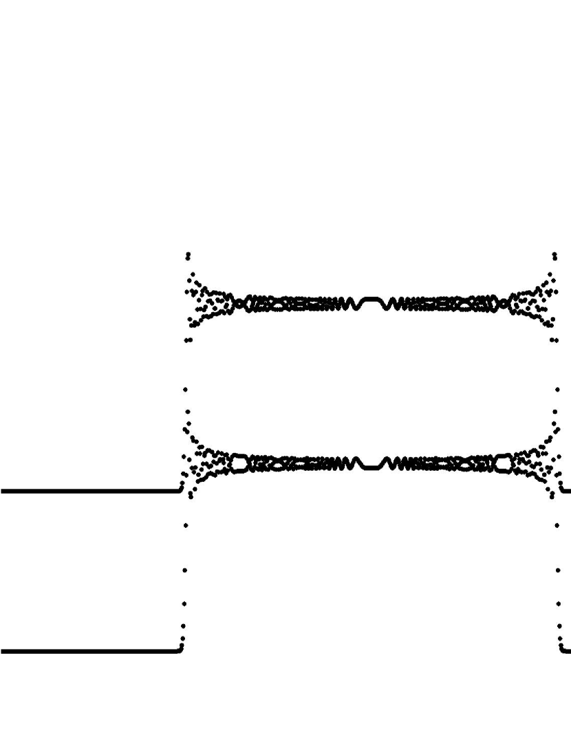
(b) $t=500$

Figure 9. Two snapshots at times $t=250$ (A) and $t=500$ (B) of the (numerically computed) solution of a harmonic lattice with periodic background initial condition.

Next, we continue with some pictures of FPUT$-\alpha$ and $\beta$ potentials and small values of these parameters (it can be said that these constitute small perturbations of the linear harmonic lattice). More precisely, for the FPUT$-\alpha$ potential and for $\alpha=0.25$, we have

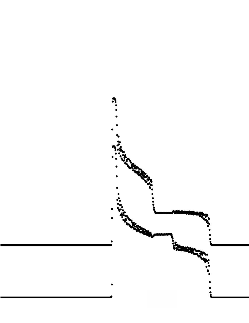
(a) $t=300$

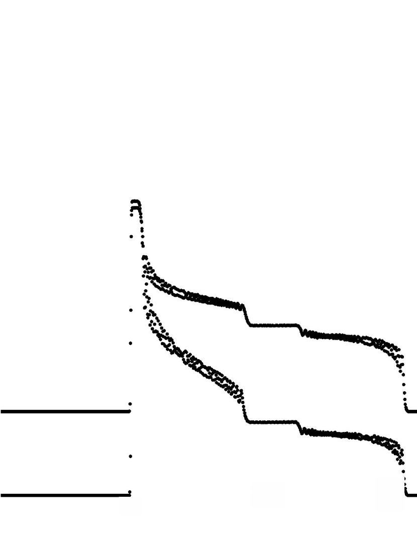
(b) $t=500$

Figure 10. Two snapshots at times $t=300$ (A) and $t=500$ (B) of the (numerically computed) solution of a FPUT$-\alpha$ lattice for $\alpha=0.25$ with periodic background initial condition.

In Figure 10 we observe one soliton, three pure periodic regions and two modulated oscillation regions in between, very similar to the Toda case in Figure 1. It should be added that we observe exactly the same behavior (qualitatively) in a plethora of other situations. Folowing you can find a list of these cases

• the Langmuir lattice

• the cube perturbed Langmuir chain at least for $\beta=0.01$ (or even smaller)

• $(2,1)-$Lennard-Jones potential for the values $(d,\varepsilon)=(10,10)$, $(1,10)$ and $(0.5,10)$

• Morse potential for the parameter values $(\gamma,\delta)=(4,1)$, $(4,0.5)$, $(4,0.25)$, $(4,0.01)$, $(8,1)$, $(8,0.5)$, $(8,0.25)$, $(8,0.1)$, $(8,0.1)$ and $(8,0.01)$

• both of the perturbed Toda potentials for small values ($0.01$ or smaller) of the parameters $\alpha$ and $\beta$ causing the perturbation

For a FPUT$-\beta$ chain with $\beta=0.01$ and periodic background, the simulations return the following figures

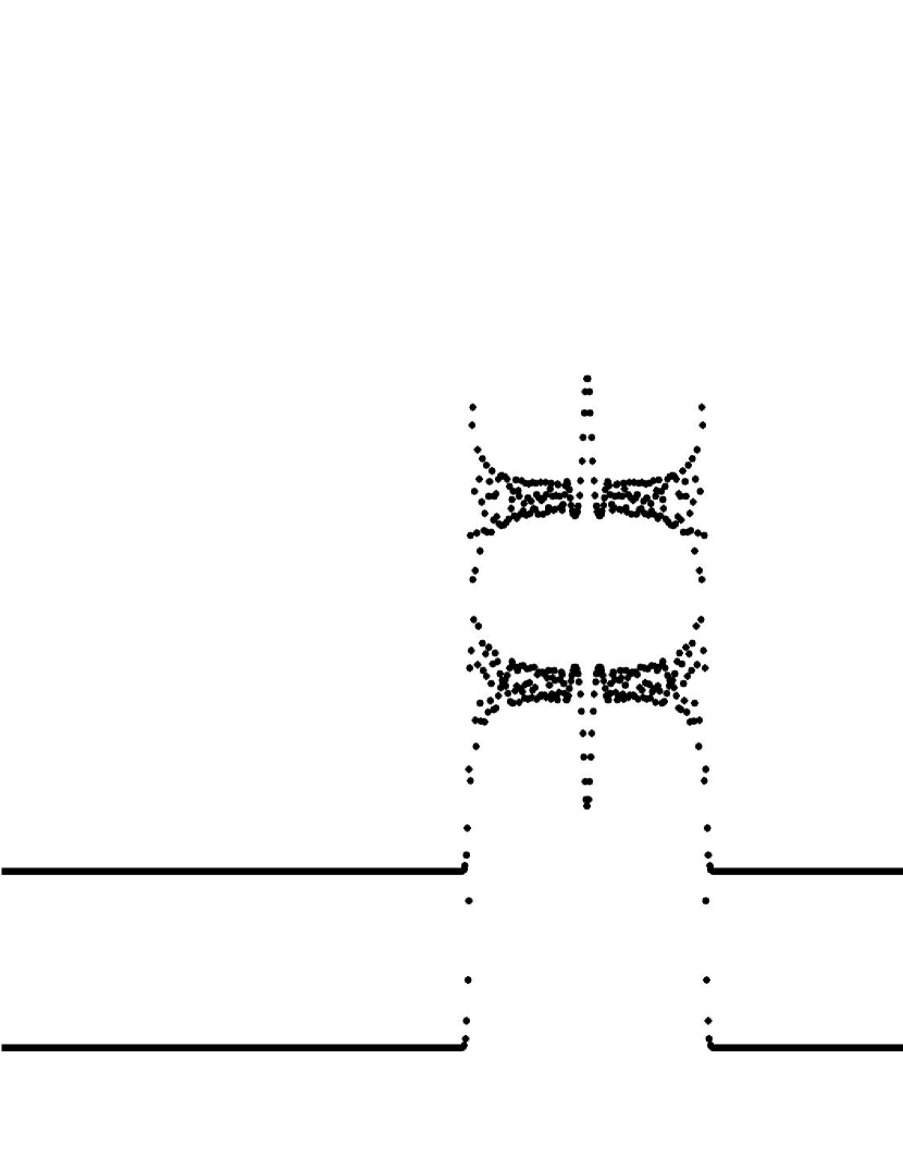
(a) $t=200$

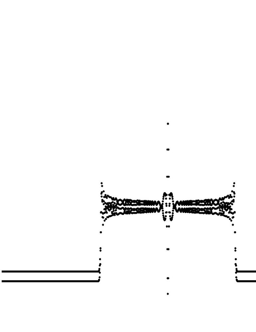
(b) $t=400$

Figure 11. Two snapshots at times $t=200$ (A) and $t=400$ (B) of the (numerically computed) solution of a FPUT$-\beta$ lattice for $\beta=0.01$ with periodic background initial condition.

In this case, there are two traveling solitons and one breather. There are also pure periodic regions in between.

Although small perturbations of the completely integrable cases still give the same picture (i.e. pure periodicity plus modulations plus solitons), for larger perturbations this picture becomes more complicated. Even chaos can possibly appear.

5. Conclusion

We have investigated a soliton resolution conjecture for FPUT lattices in a constant or periodic background and we have presented numerical computations supporting such a conjecture in the case of a FPUT lattice, for small perturbations of completely integrable one-dimensional lattices, but not necessarily for larger perturbations. For the exact Toda, the computations have already been done many years ago in [10] and complete proofs already exist ([11], [12]).

To make the conjecture more precise:

Soliton Resolution Conjecture.

Consider the solution of the initial value problem for the FPUT nearest neighbour lattice in one dimension which is a small perturbation of the linear harmonic lattice or the Toda lattice or in fact any integrable lattice, with initial data which is asymptotically periodic in space. Then, we have the following facts asymptotically:

1. The $(n,t)$-space, splits into two kinds of regions separated by straight lines passing through the origin.

2. There are regions of periodicity (the period being equal to the period of the background), and then there are regions where the PDE or lattice undergoes modulated oscillations with large (order $1/t$) frequency and slowly varying (with $n/t$) amplitude and phase. Phenomena appear in two different scales and are naturally expressed in two new variables: the fast one being $1/t$ and the slow one being $n/t$. The regions of periodicity and the modulation regions are open cones bounded by half-lines (if we consider only positive times t) emerging at the origin. There may also be solitons: travelling waves with constant shape and speed. The soliton regions are small (in $1/t$) regions around (some of) these half-lines. The slopes of the half-lines are the speeds of the solitons.

3. In the special case where the initial data background is constant the modulated oscillations region does not occur.

Remark 5.1.

The conjecture is most certainly true when the forces between adjacent particles render the lattices integrable. Even though proofs have not been produced for all possible such lattices it is pretty clear that the inverse scattering – Riemann-Hilbert methods will produce the same results. It is now also confirmed numerically when a small extra term is added to these forces even if integrability via inverse scattering is destroyed. On the other hand general lattices away from integrable cases above can exhibit a much less regular, even chaotic behaviour.

Remark 5.2.

The above conclusion raises the following question. How can (and why) the soliton resolution conjecture be valid for any PDE of dispersive type and not for all Hamiltonian lattices with forces between adjacent particles?

We admit that the answer to this question eludes at this point!

Remark 5.3.

We also believe that similar phenomena will appear in higher space dimensions. But it remains to be seen what kind of coherent structures appear in place of the simple trivial background solitons.

Remark 5.4.

Back in the last decade where the soliton resolution conjecture was first generalised to non-integrable NLS-type equations it was only deemed realistic to consider a trivial background ([15]). In view of the recent flurry of activity involving rogue wave phenomena, which only exist for non-trivial backgrounds and have only been rigorously treated in the case of a periodic background, we feel that a generalisation to periodic background deserves to be considered. A background with an indefinite reservoir of energy is very realistic when one considers, say, the huge oceans.

Appendix A Long Time Asymptotics of the Periodic Toda Lattice under Short-Range Perturbations and the Riemann-Hilbert method

We summarise here the most important results of [11]. Consider the doubly infinite Toda lattice in Flaschka’s variables

(A.1) $$\dot{b}(n,t) =2\Big{[}a(n,t)^{2}-a(n-1,t)^{2}\Big{]},$$

$$\dot{a}(n,t) =a(n,t)\Big{[}b(n+1,t)-b(n,t)\Big{]},\quad(n,t)\in{\mathbb{Z}}\times{\mathbb{R}}$$

where the dot denotes differentiation with respect to time and $a(n,t)$, $b(n,t)$ are the Flaschka variables

(A.2) $$a(n,t) =\frac{1}{2}\exp\Big{\{}\tfrac{1}{2}\big{[}x(n,t)-x(n+1,t)\big{]}\Big{\}}$$

$$b(n,t) =-\frac{1}{2}\dot{x}(n,t),$$

In this appendix we will consider a periodic algebro-geometric background solution $(a_{q},b_{q})$ to be described in a while in the next paragraph, plus a short-range perturbation $(a,b)$ satisfying

(A.3) $$\sum_{n\in{\mathbb{Z}}}\Big{[}n^{6}\big{(}|a(n,t)-a_{q}(n,t)|+|b(n,t)-b_{q}(n,t)|\big{)}\Big{]}<\infty$$

for $t=0$ and hence for all $t\in{\mathbb{R}}$. The perturbed solution can be analysed with the help of the inverse scattering transform in a periodic background ([7]).

To fix our background solution, consider a hyperelliptic Riemann surface of genus $g$ with real moduli $E_{0},E_{1},...,E_{2g+1}$. Choose a Dirichlet divisor $\mathcal{D}_{\underline{\hat{\mu}}}$ and introduce

(A.4) $$\underline{z}(n,t)=\underline{\hat{A}}_{p_{0}}(\infty_{+})-\underline{\hat{\alpha}}_{p_{0}}(\mathcal{D}_{\underline{\hat{\mu}}})-n\underline{\hat{A}}_{\infty_{-}}(\infty_{+})+t\underline{U}_{0}-\underline{\hat{\Xi}}_{p_{0}}\in{\mathbb{C}}^{g},$$

where $\underline{A}_{p_{0}}$ ($\underline{\alpha}_{p_{0}}$) is Abel’s map (for divisors) and $\underline{\Xi}_{p_{0}}$, $\underline{U}_{0}$ are some properly defined constants. Then our background solution is given in terms of Riemann theta functions by

$$a_{q}(n,t)^{2} =\tilde{a}^{2}\frac{\theta(\underline{z}(n+1,t))\theta(\underline{z}(n-1,t))}{\theta(\underline{z}(n,t))^{2}},$$

(A.5) $$b_{q}(n,t) =\tilde{b}+\frac{1}{2}\frac{d}{dt}\log\Bigg{[}\frac{\theta(\underline{z}(n,t))}{\theta(\underline{z}(n-1,t))}\Bigg{]},$$

where $\tilde{a}$, $\tilde{b}\in{\mathbb{R}}$ are again some constants.

We can of course view this hyperelliptic Riemann surface as formed by cutting and pasting two copies of the complex plane along bands. Having this picture in mind, we denote the standard projection to the complex plane by $\boldsymbol{\pi}$.

Assume for simplicity that the Jacobi operator

(A.6) $$H(t)f(n)=a(n,t)f(n+1)+a(n-1,t)f(n-1)+b(n,t)f(n),\quad f\in\ell^{2}({\mathbb{Z}}),$$

corresponding to the perturbed problem (A.1) has no eigenvalues. Then, for long times the perturbed Toda lattice is asymptotically close to the following limiting lattice defined by

(A.7) $$\prod_{j=n}^{\infty}\Bigg{[}\frac{a_{l}(j,t)}{a_{q}(j,t)}\Bigg{]}^{2}=\frac{\theta(\underline{z}(n,t))}{\theta(\underline{z}(n-1,t))} \frac{\theta(\underline{z}(n-1,t)+\underline{\delta}(n,t))}{\theta(\underline{z}(n,t)+\underline{\delta}(n,t))}\times$$

$$\times\exp\left(\frac{1}{2\pi\mathrm{i}}\int_{C(n/t)}\log(1-|R|^{2})\omega_{\infty_{+}\,\infty_{-}}\right),$$

$$\delta_{\ell}(n,t)=\frac{1}{2\pi\mathrm{i}} \int_{C(n/t)}\log(1-|R|^{2})\zeta_{\ell},$$

where $R$ is the reflection coefficient defined when considering scattering with respect to the periodic background (see [11] for the actual definition; it encapsulates the short range perturbation), $\zeta_{\ell}$ is a canonical basis of holomorphic differentials, $\omega_{\infty_{+}\,\infty_{-}}$ is an Abelian differential of the third kind defined in (B.15), and $C(n/t)$ is a contour on the Riemann surface. More specific, $C(n/t)$ is obtained by taking the spectrum of the unperturbed Jacobi operator $H_{q}$ between $-\infty$ and a special stationary phase point $z_{j}(n/t)$, for the phase of the underlying Riemann–Hilbert problem (see below), and lifting it to the Riemann surface (oriented such that the upper sheet lies to its left). The point $z_{j}(n/t)$ will move from $-\infty$ to $+\infty$ as $n/t$ varies from $-\infty$ to $+\infty$. From the products above, one easily recovers $a_{l}(n,t)$. More precisely, from [11] we have the following:

Theorem A.1.

Let $C$ be any (large) positive number and $\delta$ be any (small) positive number. Consider the region $D=\{(n,t):|\frac{n}{t}|<C\}$. Then one has

(A.8) $$\prod_{j=n}^{\infty}\frac{a_{l}(j,t)}{a(j,t)}\to 1$$

uniformly in $D$, as $t\to\infty$.

A similar theorem can be proved for the velocities $b(n,t)$:

Theorem A.2.

In the region $D=\{(n,t):|\frac{n}{t}|<C\},$ of Theorem  A.1 we also have

(A.9) $$\sum_{j=n}^{\infty}\big{[}b_{l}(j,t)-b_{q}(j,t)\big{]}\to 0$$

uniformly in $D$, as $t\to\infty$, where $b_{l}$ is given by

(A.10) $$\sum_{j=n}^{\infty}\big{[}b_{l}(j,t)-b_{q}(j,t)\big{]}= \frac{1}{2\pi\mathrm{i}}\int_{C(n/t)}\log(1-|R|^{2})\Omega_{0}$$

$${}+\frac{1}{2}\frac{d}{ds}\log\left(\frac{\theta(\underline{z}(n,s)+\underline{\delta}(n,t))}{\theta(\underline{z}(n,s))}\right)\Bigg{|}_{s=t}$$

and $\Omega_{0}$ is an Abelian differential of the second kind defined in (B.16).

Remark A.3.

(i) It is easy to see how the asymptotic formulae above describe the picture given by the numerics. Recall that the spectrum $\sigma(H_{q})$ of $H_{q}$ consists of $g+1$ bands whose band edges are the branch points of the underlying hyperelliptic Riemann surface. If $\frac{n}{t}$ is small enough, $z_{j}(n/t)$ is to the left of all bands implying that $C(n/t)$ is empty and thus $\delta_{\ell}(n,t)=0$; so we recover the purely periodic lattice. At some value of $\frac{n}{t}$ a stationary phase point first appears in the first band of $\sigma(H_{q})$ and begins to move from the left endpoint of the band towards the right endpoint of the band. (More precisely we have a pair of stationary phase points $z_{j}$ and $z_{j}^{*}$, one in each sheet of the hyperelliptic curve, with common projection $\boldsymbol{\pi}(z_{j})$ on the complex plane.) So $\delta_{\ell}(n,t)$ is now a non-zero quantity changing with $\frac{n}{t}$ and the asymptotic lattice has a slowly modulated non-zero phase. Also the factor given by the exponential of the integral is non-trivially changing with $\frac{n}{t}$ and contributes to a slowly modulated amplitude. Then, after the stationary phase point leaves the first band there is a range of $\frac{n}{t}$ for which no stationary phase point appears in the spectrum $\sigma(H_{q})$, hence the phase shift $\delta_{\ell}(n,t)$ and the integral remain constant, so the asymptotic lattice is periodic (but with a non-zero phase shift). Eventually a stationary phase point appears in the second band, so a new modulation appears and so on. Finally, when $\frac{n}{t}$ is large enough, so that all bands have been traversed by the stationary phase point(s), the asymptotic lattice is again periodic. Periodicity properties of theta functions easily show that phase shift is actually cancelled by the exponential of the integral and we recover the original periodic lattice with no phase shift at all.

(ii) If eigenvalues are present one can apply appropriate Darboux transformations to add the effect of such eigenvalues. Alternatively one can modify the Riemann-Hilbert problem by adding small circles around the extra poles coming from the eigenvalues and applying some of the methods in [5]. What we then see asymptotically is travelling solitons in a periodic background. Note that this will change the asymptotics on one side. More precisely we have (see [12]) the following formulae:

Theorem A.4.

Assume (A.3) and denote the eigenvalues of the Jacobi operatror by $\rho_{k},~{}~{}~{}k=1,....,N$. Let $c_{k}=v(\rho_{k})$ (the velocity of the $k^{th}$ soliton) defined via

(A.11) $$v(\lambda)=\lim_{\varepsilon\to 0}\frac{-\mathrm{Re}\int_{E_{0}}^{(\lambda+\mathrm{i}\varepsilon,+)}\!\Omega_{0}}{\mathrm{Re}\int_{E_{0}}^{(\lambda+\mathrm{i}\varepsilon,+)}\!\omega_{\infty_{+}\,\infty_{-}}},$$

where $\Omega_{0}$ is an Abelian differential of the second kind defined in (B.16) and $\omega_{\infty_{+}\,\infty_{-}}$ is the Abelian differential of the third kind with poles at $\infty_{+}$ and $\infty_{-}$ defined in (B.15). Also let $\varepsilon>0$ sufficiently small such that the intervals $[c_{k}-\varepsilon,c_{k}+\varepsilon]$, $1\leq k\leq N$, are disjoint and lie inside $v\big{(}{\mathbb{R}}\backslash\sigma(H_{q})\big{)}$. Then the asymptotics in the soliton region, $\{(n,t)|\,\zeta(n/t)\in{\mathbb{R}}\backslash\sigma(H_{q})\}$, are as follows:

• if $|\frac{n}{t}-c_{k}|<\varepsilon$ for some $k$, the solution is asymptotically given by a one-soliton solution on top of the limiting lattice:

  $$\prod_{j=n}^{\infty}\frac{a(j,t)}{a_{l}(j,t)} =\left(\sqrt{\frac{c_{l,\gamma_{k}(n,t)}(\rho_{k},n-1,t)}{c_{l,\gamma_{k}(n,t)}(\rho_{k},n,t)}}+O(t^{-l})\right),$$

  (A.12) $$\sum_{j=n+1}^{\infty}b(j,t)-b_{l}(j,t) =-\gamma_{k}(n,t)\frac{a_{l}(n,t)\psi_{l}(\rho_{k},n,t)\psi_{l}(\rho_{k},n+1,t)}{2c_{l,\gamma_{k}(n,t)}(\rho_{k},n,t)}+O(t^{-l}),$$

  for any $l\geq 1$, where

  (A.13) $$c_{l,\gamma}(\rho,n,t)=1+\gamma\!\!\sum_{j=n+1}^{\infty}\psi_{l,+}(\rho,j,t)^{2}$$

  and

  (A.14) $$\gamma_{k}(n,t)=\gamma_{k}\frac{T(\rho_{k}^{*},n,t)}{T(\rho_{k},n,t)}.$$

• if $|\frac{n}{t}-c_{k}|\geq\varepsilon$, for all $k$, the solution is asymptotically close to the limiting lattice:

  $$\prod_{j=n}^{\infty}\frac{a(j,t)}{a_{l}(j,t)} =1+O(t^{-l}),$$

  (A.15) $$\sum_{j=n+1}^{\infty}b(j,t)-b_{l}(j,t) =O(t^{-l}),$$

  for any $l\geq 1$.

Here $\psi_{l}(p,n,t)$ is the Baker-Akhiezer function (cf. Section B) corresponding to the limiting lattice defined above. The suffix $\pm$ refers to the restriction on the $\pm$ sheet and the star denotes sheet flipping. $T$ is the transition coefficient defined when considering scattering with respect to the periodic background.

(iii) It is very easy to also show that in any region $|\frac{n}{t}|>C$, one has

(A.16) $$\prod_{j=n}^{\infty}\frac{a_{l}(j,t)}{a(j,t)}\to 1$$

uniformly in $t$, as $n\to\infty$.

By dividing in (A.7) one recovers the $a(n,t)$. It follows from the theorem above that

(A.17) $$|a(n,t)-a_{l}(n,t)|\to 0$$

uniformly in $D$, as $t\to\infty$. In other words, the perturbed Toda lattice is asymptotically close to the limiting lattice above.

The proof is based on a stationary phase type argument. One reduces the given Riemann-Hilbert problem to a localised parametrix Riemann-Hilbert problem. This is done via the solution of a scalar global Riemann-Hilbert problem which is solved explicitly with the help of the Riemann-Roch theorem. The reduction to a localised parametrix Riemann-Hilbert problem is done with the help of a theorem reducing general Riemann-Hilbert problems to singular integral equations. (A generalized Cauchy transform is defined appropriately for each Riemann surface.) The localised parametrix Riemann-Hilbert problem is solved explicitly in terms of parabolic cylinder functions. The argument follows [4] up to a point but also extends the theory of Riemann-Hilbert problems for Riemann surfaces. The right (well-posed) Riemann-Hilbert factorisation problems are no more holomorphic but instead have a number of poles equal to the genus of the surface.

Appendix B Algebro-geometric quasi-periodic finite-gap solutions

We present some facts on our background solution $(a_{q},b_{q})$ which we want to choose from the class of algebro-geometric quasi-periodic finite-gap solutions, that is the class of stationary solutions of the Toda hierarchy. In particular, this class contains all periodic solutions. We will use the same notation as in [16], where we also refer to for proofs.

To set the stage let ${\mathbb{M}}$ be the Riemann surface associated with the following function

(B.1) $$R_{2g+2}^{1/2}(z),\qquad R_{2g+2}(z)=\prod_{j=0}^{2g+1}(z-E_{j}),\qquad E_{0}<E_{1}<\cdots<E_{2g+1},$$

$g\in{\mathbb{N}}$. ${\mathbb{M}}$ is a compact, hyperelliptic Riemann surface of genus $g$. We will choose $R_{2g+2}^{1/2}(z)$ as the fixed branch

(B.2) $$R_{2g+2}^{1/2}(z)=-\prod_{j=0}^{2g+1}\sqrt{z-E_{j}},$$

where $\sqrt{.}$ is the standard root with branch cut along $(-\infty,0)$.

A point on ${\mathbb{M}}$ is denoted by $p=\big{(}z,\pm R_{2g+2}^{1/2}(z)\big{)}=(z,\pm)$, $z\in{\mathbb{C}}$, or $p=(\infty,\pm)=\infty_{\pm}$, and the projection onto ${\mathbb{C}}\cup\{\infty\}$ by $\boldsymbol{\pi}(p)=z$. The points $\{(E_{j},0),0\leq j\leq 2g+1\}\subseteq{\mathbb{M}}$ are called branch points and the sets

(B.3) $$\Pi_{\pm}=\{\big{(}z,\pm R_{2g+2}^{1/2}(z)\big{)}\big{|}z\in{\mathbb{C}}\setminus\bigcup_{j=0}^{g}[E_{2j},E_{2j+1}]\}\subset{\mathbb{M}}$$

are called upper, lower sheet, respectively.

Let $\{a_{j},b_{j}\}_{j=1}^{g}$ be loops on the surface ${\mathbb{M}}$ representing the canonical generators of the fundamental group $\boldsymbol{\pi}_{1}({\mathbb{M}})$. We require $a_{j}$ to surround the points $E_{2j-1}$, $E_{2j}$ (thereby changing sheets twice) and $b_{j}$ to surround $E_{0}$, $E_{2j-1}$ counterclockwise on the upper sheet, with pairwise intersection indices given by

(B.4) $$a_{i}\circ a_{j}=b_{i}\circ b_{j}=0,\qquad a_{i}\circ b_{j}=\delta_{i,j},\qquad 1\leq i,j\leq g.$$

The corresponding canonical basis $\{\zeta_{j}\}_{j=1}^{g}$ for the space of holomorphic differentials can be constructed by

(B.5) $$\underline{\zeta}=\sum_{j=1}^{g}\underline{c}(j)\frac{\boldsymbol{\pi}^{j-1}d\boldsymbol{\pi}}{R_{2g+2}^{1/2}},$$

where the constants $\underline{c}(.)$ are given by

(B.6) $$c_{j}(k)=C_{jk}^{-1},\qquad C_{jk}=\int_{a_{k}}\frac{\boldsymbol{\pi}^{j-1}d\boldsymbol{\pi}}{R_{2g+2}^{1/2}}=2\int_{E_{2k-1}}^{E_{2k}}\frac{z^{j-1}dz}{R_{2g+2}^{1/2}(z)}\in{\mathbb{R}}.$$

The differentials fulfill

(B.7) $$\int_{a_{j}}\zeta_{k}=\delta_{j,k},\qquad\int_{b_{j}}\zeta_{k}=\tau_{j,k},\qquad\tau_{j,k}=\tau_{k,j},\qquad 1\leq j,k\leq g.$$

Now pick $g$ numbers (the Dirichlet eigenvalues)

(B.8) $$(\hat{\mu}_{j})_{j=1}^{g}=(\mu_{j},\sigma_{j})_{j=1}^{g}$$

whose projections lie in the spectral gaps, that is, $\mu_{j}\in[E_{2j-1},E_{2j}]$. Associated with these numbers is the divisor $\mathcal{D}_{\underline{\hat{\mu}}}$ which is one at the points $\hat{\mu}_{j}$ and zero else. Using this divisor we introduce

$$\underline{z}(p,n,t) =\underline{\hat{A}}_{p_{0}}(p)-\underline{\hat{\alpha}}_{p_{0}}(\mathcal{D}_{\underline{\hat{\mu}}})-n\underline{\hat{A}}_{\infty_{-}}(\infty_{+})+t\underline{U}_{0}-\underline{\hat{\Xi}}_{p_{0}}\in{\mathbb{C}}^{g},$$

(B.9) $$\underline{z}(n,t) =\underline{z}(\infty_{+},n,t),$$

where $\underline{\Xi}_{p_{0}}$ is the vector of Riemann constants

(B.10) $$\hat{\Xi}_{p_{0},j}=\frac{j+\sum_{k=1}^{g}\tau_{j,k}}{2},\qquad p_{0}=(E_{0},0),$$

$\underline{U}_{0}$ are the b-periods of the Abelian differential $\Omega_{0}$ defined below, and $\underline{A}_{p_{0}}$ ($\underline{\alpha}_{p_{0}}$) is Abel’s map (for divisors). The hat indicates that we regard it as a (single-valued) map from $\hat{{\mathbb{M}}}$ (the fundamental polygon associated with ${\mathbb{M}}$ by cutting along the $a$ and $b$ cycles) to ${\mathbb{C}}^{g}$. We recall that the function $\theta(\underline{z}(p,n,t))$ has precisely $g$ zeros $\hat{\mu}_{j}(n,t)$ (with $\hat{\mu}_{j}(0,0)=\hat{\mu}_{j}$), where $\theta(\underline{z})$ is the Riemann theta function of ${\mathbb{M}}$.

Then our background solution is given by

$$a_{q}(n,t)^{2} =\tilde{a}^{2}\frac{\theta(\underline{z}(n+1,t))\theta(\underline{z}(n-1,t))}{\theta(\underline{z}(n,t))^{2}},$$

(B.11) $$b_{q}(n,t) =\tilde{b}+\frac{1}{2}\frac{d}{dt}\log\Big{[}\frac{\theta(\underline{z}(n,t))}{\theta(\underline{z}(n-1,t))}\Big{]}.$$

The constants $\tilde{a}$, $\tilde{b}$ depend only on the Riemann surface (see [16] section $9.2$).

Introduce the time dependent Baker-Akhiezer function

(B.12) $$\psi_{q}(p,n,t) =C(n,0,t)\frac{\theta(\underline{z}(p,n,t))}{\theta(\underline{z}(p,0,0))}\exp\Big{(}n\int_{E_{0}}^{p}\omega_{\infty_{+}\,\infty_{-}}+t\int_{E_{0}}^{p}\Omega_{0}\Big{)},$$

where $C(n,0,t)$ is real-valued,

(B.13) $$C(n,0,t)^{2}=\frac{\theta(\underline{z}(0,0))\theta(\underline{z}(-1,0))}{\theta(\underline{z}(n,t))\theta(\underline{z}(n-1,t))},$$

and the sign has to be chosen in accordance with $a_{q}(n,t)$. Here

(B.14) $$\theta(\underline{z})=\sum_{\underline{m}\in{\mathbb{Z}}^{g}}\exp\Big{\{}2\pi\mathrm{i}\left(\langle\underline{m},\underline{z}\rangle+\frac{\langle\underline{m},\underline{\tau}\,\underline{m}\rangle}{2}\right)\Big{\}},\qquad\underline{z}\in{\mathbb{C}}^{g},$$

is the Riemann theta function associated with ${\mathbb{M}}$,

(B.15) $$\omega_{\infty_{+}\,\infty_{-}}=\frac{\prod_{j=1}^{g}(\boldsymbol{\pi}-\lambda_{j})}{R_{2g+2}^{1/2}}d\boldsymbol{\pi}$$

is the Abelian differential of the third kind with poles at $\infty_{+}$ and $\infty_{-}$ and

(B.16) $$\Omega_{0}=\frac{\prod_{j=0}^{g}(\boldsymbol{\pi}-\tilde{\lambda}_{j})}{R_{2g+2}^{1/2}}d\boldsymbol{\pi},\qquad\sum_{j=0}^{g}\tilde{\lambda}_{j}=\frac{1}{2}\sum_{j=0}^{2g+1}E_{j},$$

is the Abelian differential of the second kind with second order poles at $\infty_{+}$ respectively $\infty_{-}$ (see [16, Sects. 13.1, 13.2]). All Abelian differentials are normalized to have vanishing $a_{j}$ periods.

The Baker-Akhiezer function is a meromorphic function on ${\mathbb{M}}\setminus\{\infty_{\pm}\}$ with an essential singularity at $\infty_{\pm}$. The two branches are denoted by

(B.17) $$\psi_{q,\pm}(z,n,t)=\psi_{q}(p,n,t),\qquad p=(z,\pm)$$

and it satisfies

$$H_{q}(t)\psi_{q}(p,n,t) =\boldsymbol{\pi}(p)\psi_{q}(p,n,t),$$

(B.18) $$\frac{d}{dt}\psi_{q}(p,n,t) =P_{q,2}(t)\psi_{q}(p,n,t),$$

where

(B.19) $$H_{q}(t)f(n) =a_{q}(n,t)f(n+1)+a_{q}(n-1,t)f(n-1)+b_{q}(n,t)f(n),$$

(B.20) $$P_{q,2}(t)f(n) =a_{q}(n,t)f(n+1)-a_{q}(n-1,t)f(n-1)$$

are the operators from the Lax pair for the Toda lattice.

It is well known that the spectrum of $H_{q}(t)$ is time independent and consists of $g+1$ bands

(B.21) $$\sigma(H_{q})=\bigcup_{j=0}^{g}[E_{2j},E_{2j+1}].$$

Appendix C MATLAB^® code

Here we present the code used for our simulations. The main program we ran in MATLAB^® is
clear all; close all; clc
%number of particles (a power of 2)
N=2048;
%size of time-step
DT=1;
%number of time-steps
TMAX=800;
%discretization of time-inteval
tspan=$[$0:DT:TMAX$]$;
%test different tolerances, changing Reltol
options=odeset(’Reltol’,1e-4,’OutputFcn’,’odeplot’,’OutputSel’,[1,2,N]);
%define initial-condition vector
%first N entries denote position & last N entries velocity
b=zeros(2*N,1);
%our two initial conditions
%we uncomment only one of them each time we run this code
for I=1:N
%zero background initial conditions
%b(I)=exp(-((I-N/4)/4)^2); b(I+N)=0;
%periodic background initial condition
%b(I)=0; b(I+N)=(-1)^I+2*(I==N/2);
end
%time integration method
$[$t,y$]$=ode45(’diffsystem’,tspan,b,options,N);

where the function diffsystem is defined as follows
function $[$db$]$=diffsystem(t,b)
%number of particles (a power of 2)
N=2048;
for K=1:N
D(K)=b(N+K);
end
%the function p in what follows represents the potential function we consider
%in each case (e.g. Toda potential) and is defined in another file
D(N+1)=p(b(2)-b(1))-p(b(1)-b(N));
for L=2:N-1
D(N+L)=p(b(L+1)-b(L))-p(b(L)-b(L-1));
end
D(2*N)=p(b(1)-b(N))-p(b(N)-b(N-1));
db=D’;
end

References

- [1] M.J. Ablowitz, H. Segur, Asymptotic solutions of the Korteweg–de Vries equation, Studies in Appl. Math. 57-1, 13–44, (1976/77).
- [2] S. Chatterjee, Invariant Measures and the Soliton Resolution Conjecture, Comm. in Pure and Applied Math. 67, 1737–1842 (2014).
- [3] T. Dauxois, M. Peyrard and S. Ruffo, The Fermi–Pasta–Ulam ‘numerical experiment’: history and pedagogical perspectives European Journal of Physics 26, no. 5 (2005): S3.
- [4] P. Deift, X. Zhou, A steepest descent method for oscillatory Riemann–Hilbert problems, Ann. of Math. (2) 137, 295–368 (1993).
- [5] P. Deift, S. Kamvissis, T. Kriecherbauer, X. Zhou,The Toda rarefaction problem, Comm. in Pure and Applied Math. 49 35–83 (1996).
- [6] P. Deift, S. Venakides, and X. Zhou, The collisionless shock region for the long time behavior of solutions of the KdV equation, Comm. in Pure and Applied Math. 47, 199–206 (1994).
- [7] I. Egorova, J. Michor, and G. Teschl, Scattering theory for Jacobi operators with quasi-periodic background, Comm. Math. Phys. 264-3, 811–842 (2006).
- [8] S. Kamvissis, On the long time behavior of the doubly infinite Toda lattice under initial data decaying at infinity, Comm. Math. Phys., 153-3, 479–519 (1993).
- [9] S. Kamvissis, Long time behavior for the focusing nonlinear Schrödinger equation with real spectral singularities, Comm. Math. Phys., 180-2, 325–343 (1996).
- [10] S. Kamvissis and G. Teschl, Stability of periodic soliton equations under short range perturbations, Phys. Lett. A, 364-6, 480–483 (2007).
- [11] S. Kamvissis and G. Teschl, Long-Time Asymptotics of the Periodic Toda Lattice under Short-Range Perturbations, arXiv:math-ph/0705.0346; arXiv:0805.3847; Jour. Math. Phys. 53 073706 (2012).
- [12] H. Krüger and G. Teschl, Stability of the periodic Toda lattice in the soliton region, arXiv:0807.0244; Int. Math. Res. Not. 2009, Art. ID rnp077, 36pp (2009).
- [13] H. Krüger and G. Teschl, Long-Time Asymptotics of the Toda Lattice for Decaying Initial Data Revisited, Rev. Math. Phys. 21:1, 61-109 (2009).
- [14] V. Yu. Novokshenov and I. T. Habibullin, I.T., Nonlinear Differential-Difference Schemes Integrable by the Method of the Inverse Scattering Problem. Asymptotics of the Solution for , Soviet Math. Doklady 23 no.2 304–307 (1981).
- [15] T. Tao, https://terrytao.wordpress.com/tag/soliton-resolution-conjecture/
- [16] G. Teschl, Jacobi Operators and Completely Integrable Nonlinear Lattices, Math. Surv. and Mon. 72, Amer. Math. Soc., Rhode Island, 2000.
- [17] N. J. Zabusky and M. D. Kruskal, Interaction of solitons in a collisionless plasma and the recurrence of initial states, Phys. Rev. Lett. 15, 240–243 (1965).