Simple GNN Regularisation for 3D Molecular Property Prediction & Beyond

Abstract

In this paper we show that simple noisy regularisation can be an effective way to address GNN oversmoothing. First we argue that regularisers addressing oversmoothing should both penalise node latent similarity and encourage meaningful node representations. From this observation we derive “Noisy Nodes”, a simple technique in which we corrupt the input graph with noise, and add a noise correcting node-level loss. The diverse node level loss encourages latent node diversity, and the denoising objective encourages graph manifold learning. Our regulariser applies well-studied methods in simple, straightforward ways which allow even generic architectures to overcome oversmoothing and achieve state of the art results on quantum chemistry tasks, and improve results significantly on Open Graph Benchmark (OGB) datasets. Our results suggest Noisy Nodes can serve as a complementary building block in the GNN toolkit.

1 Introduction

Graph Neural Networks (GNNs) are a family of neural networks that operate on graph structured data by iteratively passing learned messages over the graph’s structure (Scarselli et al., 2009; Bronstein et al., 2017; Gilmer et al., 2017; Battaglia et al., 2018; Shlomi et al., 2021). While Graph Neural Networks have demonstrated success in a wide variety of tasks (Zhou et al., 2020a; Wu et al., 2020; Bapst et al., 2020; Schütt et al., 2017; Klicpera et al., 2020a), it has been proposed that in practice “oversmoothing” limits their ability to benefit from overparametrization.

Oversmoothing is a phenomenon where a GNN’s latent node representations become increasing indistinguishable over successive steps of message passing (Chen et al., 2019). Once these representations are oversmoothed, the relational structure of the representation is lost, and further message-passing cannot improve expressive capacity. We argue that the challenges of overcoming oversmoothing are two fold. First, finding a way to encourage node latent diversity; second, to encourage the diverse node latents to encode meaningful graph representations. Here we propose a simple noise regulariser, Noisy Nodes, and demonstrate how it overcomes these challenges across a range of datasets and architectures, achieving top results on OC20 IS2RS & IS2RE direct, QM9 and OGBG-PCQM4Mv1.

Our “Noisy Nodes” method is a simple technique for regularising GNNs and associated training procedures. During training, our noise regularisation approach corrupts the input graph’s attributes with noise, and adds a per-node noise correction term. We posit that our Noisy Nodes approach is effective because the model is rewarded for maintaining and refining distinct node representations through message passing to the final output, which causes it to resist oversmoothing. Like denoising autoencoders, it encourages the model to explicitly learn the manifold on which the uncorrupted input graph’s features lie, analogous to a form of representation learning. When applied to 3D molecular prediction tasks, it encourages the model to distinguish between low and high energy states. We find that applying Noisy Nodes reduces oversmoothing for shallower networks, and allows us to see improvements with added depth, even on tasks for which depth was assumed to be unhelpful.

This study’s approach is to investigate the combination of Noisy Nodes with generic, popular baseline GNN architectures. For 3D Molecular prediction we use a standard architecture working on 3D point clouds developed for particle fluid simulations, the Graph Net Simulator (GNS) (Sanchez-Gonzalez* et al., 2020), which has also been used for molecular property prediction (Hu et al., 2021b). Without using Noisy Nodes the GNS is not a competitive model, but using Noisy Nodes allows the GNS to achieve top performance on three 3D molecular property prediction tasks: the OC20 IS2RE direct task by 43% over previous work, 12% on OC20 IS2RS direct, and top results on 3 out of 12 of the QM9 tasks. For non-spatial GNN benchmarks we test a MPNN (Gilmer et al., 2017) on OGBG-MOLPCBA and OGBG-PCQM4M (Hu et al., 2021a) and again see significant improvements. Finally, we applied Noisy Nodes to a GCN (Kipf & Welling, 2016), arguably the most popular and simple GNN, trained on OGBN-Arxiv and see similar results. These results suggest Noisy Nodes can serve as a complementary GNN building block.

2 Preliminaries: Graph Prediction Problem

Let $G=(V,E,g)$ be an input graph. The nodes are $V=\{v_{1},\dots,v_{|V|}\}$, where $v_{i}\in\mathbb{R}^{d_{v}}$. The directed, attributed edges are $E=\{e_{1},\dots,e_{|E|}\}$: each edge includes a sender node index, receiver node index, and edge attribute, $e_{k}=(s_{k},r_{k},e_{k})$, respectively, where $s_{k},r_{k}\in\{1,\dots,|V|\}$ and $e_{k}\in\mathbb{R}^{d_{e}}$. The graph-level property is $g\in\mathbb{R}^{d_{g}}$.

The goal is to predict a target graph, $G^{\prime}$, with the same structure as $G$, but different node, edge, and/or graph-level attributes. We denote $\hat{G}^{\prime}$ as a model’s prediction of $G^{\prime}$. Some error metric defines quality of $\hat{G}^{\prime}$ with respect to the target $G^{\prime}$, $\text{Error}(\hat{G}^{\prime},G^{\prime})$, which the training loss terms are defined to optimize. In this paper the phrase “message passing steps” is synonymous with “GNN layers”.

3 Oversmoothing

“Oversmoothing” is when the node latent vectors of a GNN become very similar after successive layers of message passing. Once nodes are identical there is no relational information contained in the nodes, and no higher-order latent graph representations can be learned. It is easiest to see this effect with the update function of a Graph Convolutional Network with no adjacency normalization $v^{k}_{i}=\sum_{j}Wv^{k-1}_{j}$ with $j\in\textit{Neighborhood}_{v_{i}},W\in\mathbb{R}^{d_{g}\times d_{g}}$ and $k$ the layer index. As the number of applications increases, the averaging effect of the summation forces the nodes to become almost identical. However, as soon as residual connections are added we can construct a network that need not suffer from oversmoothing by setting the residual updates to zero at a similarity threshold. Similarly, multi-head attention Vaswani et al. (2017); Veličković et al. (2018) and GNNs with edge updates (Battaglia et al., 2018; Gilmer et al., 2017) can modulate node updates. As such for modern GNNs oversmoothing is primarily a “training” problem - i.e. how to choose model architectures and regularisers to encourage and preserve meaningful latent relational representations.

We can discern two desiderata for a regulariser or loss that addresses oversmoothing. First, it should penalise identical node latents. Second, it should encourage meaningful latent representations of the data. One such example may be the auto-regressive loss of transformer based language models (Brown et al. (2020)). In this case, each word (equivalent to node) prediction must be distinct, and the auto-regressive loss encourages relational dependence upon prior words. We can take inspiration from this observation to derive auxiliary losses that both have diverse node targets and encourage relational representation learning. In the following section we derive one such regulariser, Noisy Nodes.

4 Noisy Nodes

Noisy Nodes tackles the oversmoothing problem by adding a diverse noise correction target, modifying the original graph prediction problem definition in several ways. It introduces a graph corrupted by noise, $\tilde{G}=(\tilde{V},\tilde{E},\tilde{g})$, where $\tilde{v}_{i}\in\tilde{V}$ is constructed by adding noise, $\sigma_{i}$, to the input nodes, $\tilde{v}_{i}=v_{i}+\sigma_{i}$. The edges, $\tilde{E}$, and graph-level attribute, $\tilde{g}$, can either be uncorrupted by noise (i.e., $\tilde{E}=E$, $\tilde{g}=g$), calculated from the noisy nodes (for example in a nearest neighbors graph), or corrupted independent of the nodes—these are minor choices that can be informed by the specific problem setting.

Our method requires a noise correction target to prevent oversmoothing by enforcing diversity in the last layers of the GNN, which can be achieved with an auxiliary denoising autoencoder loss. For example, where the Error is defined with respect to graph-level predictions (e.g., predict the minimum energy value of some molecular system), a second output head can be added to the GNN architecture which requires denoising the inputs as targets. Alternatively, if the inputs and targets are in the same real domain as is the case for physical simulations we can adjust the target for the noise. Figure 2 demonstrates this Noisy Nodes set up. The auxiliary loss is weighted by a constant coefficient $\lambda\in\mathbb{R}$.

In Figure 2 we illustrate the impact of Noisy Nodes on oversmoothing by plotting the Mean Absolute Distance (MAD) (Chen et al., 2020) of the residual updates of each layer of an MPNN trained on the QM9 (Ramakrishnan et al., 2014) dataset, and compare it to alternative methods DropEdge (Rong et al., 2019) and DropNode (Do et al., 2021). MAD is a measure of the diversity of graph node features, often used to quantify oversmoothing, the higher the number the more diverse the node features, the lower the number the less diverse. In this plot we can see that for Noisy Nodes the node updates remain diverse for all of the layers, whereas without Noisy Nodes diversity is lost. Further analysis of MAD across seeds and with sorted layers can be seen in Appendix Figures 7 and 7 for models applied to 3D point clouds.

The Graph Manifold Learning Perspective. By using an implicit mapping from corrupted data to clean data, the Noisy Nodes objective encourages the model to learn the manifold on which the clean data lies— we speculate that the GNN learns to go from low probability graphs to high probability graphs. In the autoencoder case the GNN learns the manifold of the input data. When node targets are provided, the GNN learns the manifold of the target data (e.g. the manifold of atoms at equilibrium). We speculate that such a manifold may include commonly repeated substructures that are useful for downstream prediction tasks. A similar motivation can be found for denoising in (Vincent et al., 2010; Song & Ermon, 2019).

The Energy Perspective for Molecular Property Prediction. Local, random distortions of the geometry of a molecule at a local energy minimum are almost certainly higher energy configurations. As such, a task that maps from a noised molecule to a local energy minimum is learning a mapping from high energy to low energy. Data such as QM9 contains molecules at local minima.

Some problems have input data that is already high energy, and targets that are at equilibrium. For these datasets we can generate new high energy states by adding noise to the inputs but keeping the equilibrium target the same, Figure 2 demonstrates this approach. To preserve translation invariance we use displacements between input and target $\Delta$, the corrected target after noise is $\Delta-\sigma$.

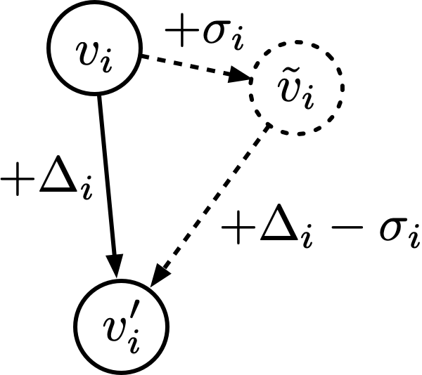
Figure 1: Noisy Node mechanics during training. Input positions are corrupted with noise $\sigma$, and the training objective is the node-level difference between target positions and the noisy inputs.

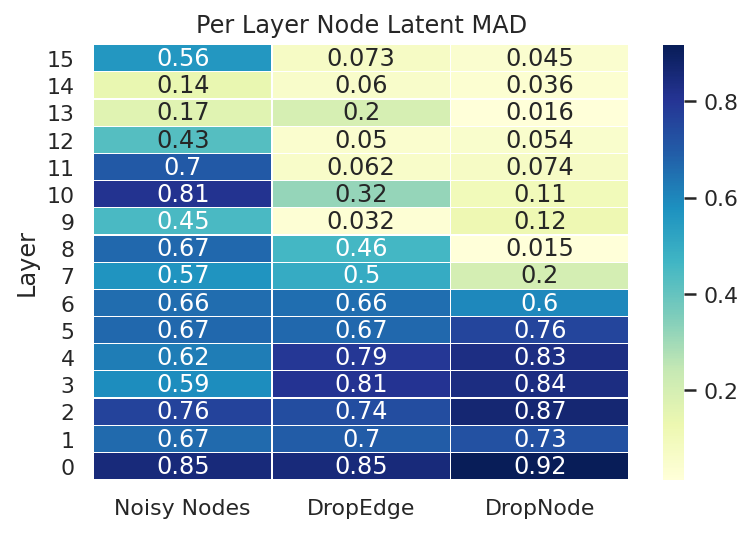
Figure 2: Per layer node latent diversity, measured by MAD on a 16 layer MPNN trained on OGBG-MOLPCBA. Noisy Nodes maintains a higher level of diversity throughout the network than competing methods.

5 Related Work

Oversmoothing. Recent work has aimed to understand why it is challenging to realise the benefits of training deeper GNNs (Wu et al., 2020). Since first being noted in ((Li et al., 2018)) oversmoothing has been studied extensively and regularisation techniques have been suggested to overcome it (Chen et al., 2019; Cai & Wang, 2020; Rong et al., 2019; Zhou et al., 2020b; Yang et al., 2020; Do et al., 2021; Zhao & Akoglu, 2020). A recent paper, (Li et al., 2021), finds, as in previous work, (Li et al., 2019; 2020), the optimal depth for some datasets they evaluate on to be far lower (5 for OGBN-Arxiv from the Open Graph Benchmark (Hu et al., 2020a), for example) than the 1000 layers possible.

Denoising & Noise Models. Training neural networks with noise has a long history (Sietsma & Dow, 1991; Bishop, 1995). Of particular relevance are Denoising Autoencoders (Vincent et al., 2008) in which an autoencoder is trained to map corrupted inputs $\tilde{\textbf{x}}$ to uncorrupted inputs x. Denoising Autoencoders have found particular success as a form of pre-training for representation learning (Vincent et al., 2010). More recently, in research applying GNNs to simulation (Sanchez-Gonzalez et al., 2018; Sanchez-Gonzalez* et al., 2020; Pfaff et al., 2020) Gaussian noise is added during training to input positions of a ground truth simulator to mimic the distribution of errors of the learned simulator. Pre-training methods (Devlin et al., 2019; You et al., 2020; Thakoor et al., 2021) are another similar approach; most similarly to our method Hu et al. (2020b) apply a reconstruction loss to graphs with masked nodes to generate graph embeddings for use in downstream tasks. FLAG (Kong et al., 2020) adds adversarial noise during training to input node features as a form of data augmentation for GNNs that demonstrates improved performance for many tasks. It does not add an additional auxiliary loss, which we find is essential for addressing oversmoothing. In other related GNN work, (Sato et al., 2021) use random input features to improve generalisation of graph neaural networks. Adding noise to help input node disambiguation has also been covered in (Dasoulas et al., 2019; Loukas, 2020; Vignac et al., 2020; Murphy et al., 2019), but there is no auxiliary loss.

Finally, we take inspiration from (Vincent et al., 2008; 2010; Vincent, 2011; Song & Ermon, 2019) which use the observation that noised data lies off the data manifold for representation learning and generative modelling.

Machine Learning for 3D Molecular Property Prediction. One application of GNNs is to speed up quantum chemistry calculations which operate on 3D positions of a molecule (Duvenaud et al., 2015; Gilmer et al., 2017; Schütt et al., 2017; Hu et al., 2021b). Common goals are the prediction of molecular properties (Ramakrishnan et al., 2014), forces (Chmiela et al., 2017), energies (Chanussot* et al., 2020) and charges (Unke & Meuwly, 2019).

A common approach to embed physical symmetries is to design a network that predicts a rotation and translation invariant energy (Schütt et al., 2017; Klicpera et al., 2020a; Liu et al., 2021). The input features of such models include distances (Schütt et al., 2017), angles (Klicpera et al., 2020b; a) or torsions and higher order terms (Liu et al., 2021). An alternative approach to embedding symmetries is to design a rotation equivariant neural network that use equivariant representations (Thomas et al., 2018; Köhler et al., 2019; Kondor et al., 2018; Fuchs et al., 2020; Batzner et al., 2021; Anderson et al., 2019; Satorras et al., 2021).

Machine Learning for Bond and Atom Molecular Graphs. Predicting properties from molecular graphs without 3D points, such as graphs of bonds and atoms, is studied separately and often used to benchmark generic graph property prediction models such as GCNs (Hu et al., 2020a) or GATs (Veličković et al., 2018). Models developed for 3D molecular property prediction cannot be applied to bond and atom graphs. Common datasets that contain such data are OGBG-MOLPCBA and OGBG-MOLHIV.

6 3D Molecular Property Prediction Experiments and Results

In this section we evaluate how a popular, simple model, the GNS (Sanchez-Gonzalez* et al., 2020) performs on 3D molecular prediction tasks when combined with Noisy Nodes. The GNS was originally developed for particle fluid simulations, but has recently been adapted for molecular property prediction (Hu et al., 2021b). We find that Without Noisy Nodes the GNS architecture is not competitive, but by using Noisy Nodes we see improved performance comparable to the use of specialised architectures.

We made minor changes to the GNS architecture. We featurise the distance input features using radial basis functions. We group layer weights, similar to grouped layers used in Jumper et al. (2021) for reduced parameter counts; for a group size of $n$ the first $n$ layer weights are repeated, i.e. the first layer with a group size of 10 has the same weights as the $\text{11}^{th}$, $\text{21}^{st}$, $\text{31}^{st}$ layers and so on. $n$ contiguous blocks of layers are considered a single group. Finally we find that decoding the intermediate latents and adding a loss after each group aids training stability. The decoder is shared across groups.

We tested this architecture on three challenging molecular property prediction benchmarks: OC20 (Chanussot* et al., 2020) IS2RS & IS2RE, and QM9 (Ramakrishnan et al., 2014). These benchmarks are detailed below, but as general distinctions, OC20 tasks use graphs 2-20x larger than QM9. While QM9 always requires graph-level prediction, one of OC20’s two tasks (IS2RS) requires node-level predictions while the other (IS2RE) requires graph-level predictions. All training details may be found in the Appendix.

6.1 Open Catalyst 2020

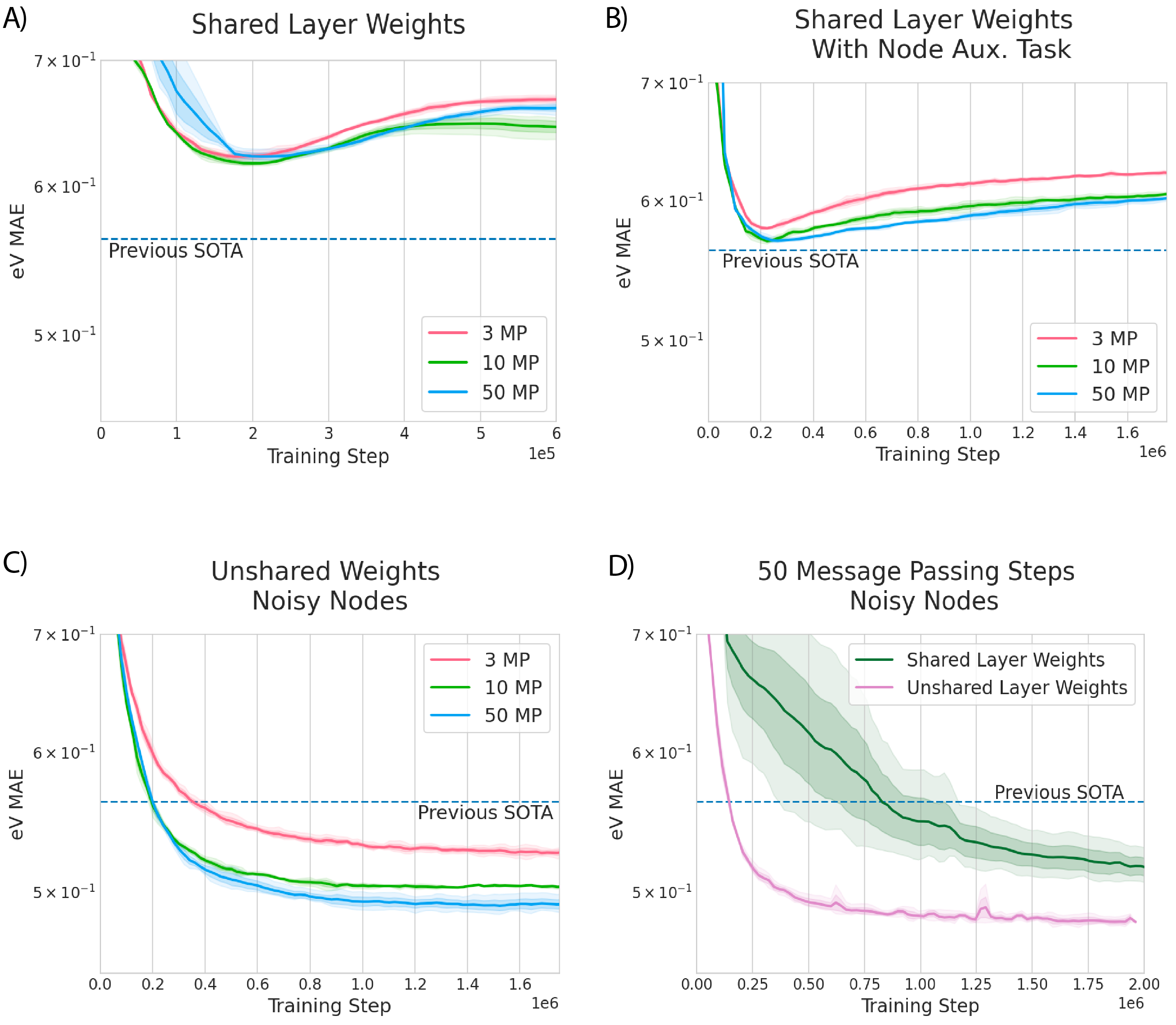
Figure 3: Validation curves, OC20 IS2RE ID. A) Without any node targets our model has poor performance and realises no benefit from depth. B) After adding a position node loss, performance improves as depth increases. C) As we add Noisy Nodes and parameters the model achieves SOTA, even with 3 layers, and stops overfitting. D) Adding Noisy Nodes allows a model with even fully shared weights to achieve SOTA.

Dataset. The OC20 dataset (Chanussot* et al., 2020) (CC Attribution 4.0) describes the interaction of a small molecule (the adsorbate) and a large slab (the catalyst), with total systems consisting of 20-200 atoms simulated until equilibrium is reached.

We focus on two tasks; the Initial Structure to Resulting Energy (IS2RE) task which takes the initial structure of the simulation and predicts the final energy, and the Initial Structure to Resulting Structure (IS2RS) which takes the initial structure and predicts the relaxed structure. Note that we train the more common “direct” prediction task that map directly from initial positions to target in a single forward pass, and compare against other models trained for direct prediction.

Models are evaluated on 4 held out test sets. Four canonical validation datasets are also provided. Test sets are evaluated on a remote server hosted by the dataset authors with a very limited number of submissions per team.

Noisy Nodes in this case consists of a random jump between the initial position and relaxed position. During training we first sample uniformly from a point in the relaxation trajectory or interpolate uniformly between the initial and final positions $(v_{i}-\tilde{v}_{i})\gamma,\gamma\sim\text{U}(0,1)$, and then add I.I.D Gaussian noise with mean zero and $\sigma=0.3$. The Noisy Node target is the relaxed structure.

We first convert to fractional coordinates (i.e. use the periodic unit cell as the basis) which render the predictions of our model invariant to rotations, and append the following rotation and translation invariant vector $(\alpha\beta^{T},\beta\gamma^{T},\alpha\gamma^{T},|\alpha|,|\beta|,|\gamma|)\in\mathbb{R}^{6}$ to the edge features where $\alpha,\beta,\gamma$ are vectors of the unit cell. This additional vector provides rotation invariant angular and extent information to the GNN.

IS2RE Results. In Figure 3 we show how using Noisy Nodes allows the GNS to achieve state of the art performance. Figure 3 A shows that without any auxiliary node target, an IS2RE GNS achieves poor performance even with increased depth. The fact that increased depth does not result in improvement supports the hypothesis that GNS suffers from oversmoothing. As we add a node level position target in B) we see better performance, and improvement as depth increases, validating our hypothesis that node level targets are key to addressing oversmoothing. In C) we add noisy nodes and parameters, and see that the increased diversity of the node level predictions leads to very significant improvements and SOTA, even for a shallow 3 layer network. D) demonstrates this effect is not just due to increased parameters - SOTA can still be achieve with shared layer weights .

In Table 1 we conduct an ablation on our hyperparameters, and again demonstrate the improved performance of using Noisy Nodes. Results were averaged over 3 seeds and standard errors on the best obtained checkpoint show little sensitivity to initialisation. All results in the table are reported using sampling states from trajectories. We conducted an ablation on ID comparing sampling from a relaxation trajectory and interpolating between initial & final positions which found that interpolation improved our score from 0.47 to 0.45.

Table 1: OC20 ISRE Validation, eV MAE, $\downarrow$.
“GNS-Shared” indicates shared weights. “GNS-10” indicates a group size of 10.

Model	Layers	OOD Both	OOD Adsorbate	OOD Catalyst	ID
GNS	50	0.59 $\pm 0.01$	0.65 $\pm 0.01$	0.55 $\pm 0.00$	0.54 $\pm 0.00$
GNS-Shared + Noisy Nodes	50	0.49 $\pm 0.00$	0.54 $\pm 0.00$	0.51 $\pm 0.01$	0.51 $\pm 0.01$
GNS + Noisy Nodes	50	0.48 $\pm 0.00$	0.53 $\pm 0.00$	0.49 $\pm 0.01$	0.48 $\pm 0.00$
GNS-10 + Noisy Nodes	100	0.46$\pm 0.00$	0.51 $\pm 0.00$	0.48 $\pm 0.00$	0.47 $\pm 0.00$

Our best hyperparameter setting was 100 layers which achieved a 95.6% relative performance improvement against SOTA results (Table 2) on the AEwT benchmark. Due to limited permitted test submissions, results presented here were from one test upload of our best performing validation seed.

Table 2: Results OC20 IS2RE Test

	eV MAE $\downarrow$
	SchNet	DimeNet++	SpinConv	SphereNet	GNS + Noisy Nodes
OOD Both	0.704	0.661	0.674	0.638	0.465 (-24.0%)
OOD Adsorbate	0.734	0.725	0.723	0.703	0.565 (-22.8%)
OOD Catalyst	0.662	0.576	0.569	0.571	0.437 (-17.2%)
ID	0.639	0.562	0.558	0.563	0.422 (-18.8%)
	Average Energy within Threshold (AEwT) $\uparrow$
	SchNet	DimeNet++	SpinConv	SphereNet	GNS + Noisy Nodes
OOD Both	0.0221	0.0241	0.0233	0.0241	0.047 (+95.8%)
OOD Adsorbate	0.0233	0.0207	0.026	0.0229	0.035 (+89.5%)
OOD Catalyst	0.0294	0.0410	0.0382	0.0409	0.080 (+95.1%)
ID	0.0296	0.0425	0.0408	0.0447	0.091 (+102.0%)

IS2RS Results. In Table 4 we see that GNS + Noisy Nodes is significantly better than the only other reported IS2RS direct result, ForceNet, itself a GNS variant.

Table 3: OC20 IS2RS Validation, ADwT, $\uparrow$

Model	Layers	OOD Both	OOD Adsorbate	OOD Catalyst	ID
GNS	50	43.0%$\pm 0.0$	38.0%$\pm 0.0$	37.5% $0.0$	40.0%$\pm 0.0$
GNS + Noisy Nodes	50	50.1%$\pm 0.0$	44.3%$\pm 0.0$	44.1%$\pm 0.0$	46.1% $\pm 0.0$
GNS-10 + Noisy Nodes	50	52.0%$\pm 0.0$	46.2%$\pm 0.0$	46.1% $\pm 0.0$	48.3% $\pm 0.0$
GNS-10 + Noisy Nodes + Pos only	100	54.3%$\pm 0.0$	48.3%$\pm 0.0$	48.2% $\pm 0.0$	50.0% $\pm 0.0$

Table 4: OC20 IS2RS Test, ADwT, $\uparrow$

Model	OOD Both	OOD Adsorbate	OOD Catalyst	ID
ForceNet	46.9%	37.7%	43.7%	44.9%
GNS + Noisy Nodes	52.7%	43.9%	48.4%	50.9%
Relative Improvement	+12.4%	+16.4%	+10.7%	+13.3%

6.2 QM9

Dataset. The QM9 benchmark (Ramakrishnan et al., 2014) contains 134k molecules in equilibrium with up to 9 heavy C, O, N and F atoms, targeting 12 associated chemical properties (License: CCBY 4.0). We use 114k molecules for training, 10k for validation and 10k for test. All results are on the test set. We subtract a fixed per atom energy from the target values computed from linear regression to reduce variance. We perform training in eV units for energetic targets, and evaluate using MAE. We summarise the results across the targets using mean standardised MAE (std. MAE) in which MAEs are normalised by their standard deviation, and mean standardised logMAE. Std. MAE is dominated by targets with high relative error such as $\Delta\epsilon$, whereas logMAE is sensitive to outliers such as $\left<R^{2}\right>$. As is standard for this dataset, a model is trained separately for each target.

Table 5: QM9, Impact of Noisy Nodes on GNS architecture.

	Layers	std. MAE	% Change	logMAE
GNS	10	1.17	-	-5.39
GNS + Noise But No Node Target	10	1.16	-0.9%	-5.32
GNS + Noisy Nodes	10	0.90	-23.1%	-5.58
GNS-10 + Noisy Nodes	20	0.89	-23.9%	-5.59
GNS-10 + Noisy Nodes + Invariance	30	0.92	-21.4%	-5.57
GNS-10 + Noisy Nodes	30	0.88	-24.8%	-5.60

Table 6: QM9, Test MAE, Mean & Standard Deviation of 3 Seeds Reported.

Target	Unit	SchNet	E(n)GNN	DimeNet++	SphereNet	PaiNN	GNS + Noisy Nodes
$\mu$	$\mathrm{D}$	0.033	0.029	0.030	0.027	0.012	0.025 $\pm 0.01$
$\alpha$	$\mathrm{\text{ $a_{0}$ }}^{3}$	0.235	0.071	0.043	0.047	0.045	0.052 $\pm 0.00$
$\epsilon_{\text{HOMO}}$	$\mathrm{meV}$	41	29.0	24.6	23.6	27.6	20.4 $\pm 0.2$
$\epsilon_{\text{LUMO}}$	$\mathrm{meV}$	34	25.0	19.5	18.9	20.4	18.6 $\pm 0.4$
$\Delta\epsilon$	$\mathrm{meV}$	63	48.0	32.6	32.3	45.7	28.6 $\pm 0.1$
$\left<R^{2}\right>$	$\mathrm{\text{ $a_{0}$ }}^{2}$	0.07	0.11	0.33	0.29	0.07	0.70 $\pm 0.01$
ZPVE	$\mathrm{meV}$	1.7	1.55	1.21	1.12	1.28	1.16 $\pm 0.01$
$U_{0}$	$\mathrm{meV}$	14.00	11.00	6.32	6.26	5.85	7.30 $\pm 0.12$
$U$	$\mathrm{meV}$	19.00	12.00	6.28	7.33	5.83	7.57 $\pm 0.03$
$H$	$\mathrm{meV}$	14.00	12.00	6.53	6.40	5.98	7.43$\pm 0.06$
$G$	$\mathrm{meV}$	14.00	12.00	7.56	8.0	7.35	8.30 $\pm 0.14$
$c_{\text{v}}$	$\frac{\mathrm{cal}}{\mathrm{mol}\text{\,}\mathrm{K}}$	0.033	0.031	0.023	0.022	0.024	0.025 $\pm 0.00$
std. MAE	$\mathrm{\char 37\relax}$	1.76	1.22	0.98	0.94	1.00	0.88
logMAE		-5.17	-5.43	-5.67	-5.68	-5.85	-5.60

For this dataset we add I.I.D Gaussian noise with mean zero and $\sigma=0.02$ to the input atom positions. A denoising autoencoder loss is used.

Results In Table 6 we can see that adding Noisy Nodes significantly improves results by 23.1% relative for GNS, making it competitive with specialised architectures. To understand the effect of adding a denoising loss, we tried just adding noise and found no where near the same improvement (Table 6).

A GNS-10 + Noisy Nodes with 30 layers achieves top results on 3 of the 12 targets and comparable performance on the remainder (Table 6). On the std. MAE aggregate metric GNS + Noisy Nodes performs better than all other reported results, showing that Noisy Nodes can make even a generic model competitive with models hand-crafted for molecular property prediction. The same trend is repeated for an rotation invariant version of this network that uses the principle axes of inertia ordered by eigenvalue as the co-ordinate frame (Table 5).

$\left<R^{2}\right>$, the electronic spatial extent, is an outlier for GNS + Noisy Nodes. Interestingly, we found that without noise GNS-10 + Noisy Nodes achieves 0.33 for this target. We speculate that this target is particularly sensitive to noise, and the best noise value for this target would be significantly lower than for the dataset as a whole.

7 Non-Spatial Tasks

The previous experiments use the 3D geometries of atoms, and models that operate on 3D points. However, the recipe of adding a denoising auxiliary loss can be applied to other graphs with different types of features. In this section we apply Noisy Nodes to additional datasets with no 3D points, using different GNNs, and show analagous effects to the 3D case. Details of the hyperparameters, models and training details can be found in the appendix.

7.1 OGBG-PCQM4M

This dataset from the OGB benchmarks consists of molecular graphs which consist of bonds and atom types, and no 3D or 2D coordinates. To adapt Noisy Nodes to this setting, we randomly flip node and edge features at a rate of 5% and add a reconstruction loss. We evaluate Noisy Nodes using an MPNN + Virtual Node (Gilmer et al., 2017). The test set is not currently available for this dataset.

Table 7: OGBG-PCQM4M Results

Model	Number of Layers	Using Noisy Nodes	MAE
MPNN + Virtual Node	16	Yes	0.1249 $\pm$ 0.0003
MPNN + Virtual Node	50	No	0.1236 $\pm$ 0.0001
Graphormer (Ying et al., 2021)	-	-	0.1234
MPNN + Virtual Node	50	Yes	0.1218 $\pm$ 0.0001

In Table 7 we see that for this task Noisy Nodes enables a 50 layer MPNN to reach state of the art results. Before adding Noisy Nodes, adding capacity beyond 16 layers did not improve results.

7.2 OGBG-MOLPCBA

The OGBG-MOLPCBA dataset contains molecular graphs with no 3D points, with the goal of classifying 128 biological activities. On the OGBG-MOLPCBA dataset we again use an MPNN + Virtual Node and random flipping noise. In Figure 5 we see that adding Noisy Nodes improves the performance of the base model, accentuated for deeper networks. Our 16 layer MPNN improved from 27.6% $\pm$ 0.004 to 28.1% $\pm$ 0.002 Mean Average Precision (“Mean AP”). Figure 5 demonstrates how Noisy Nodes improves performance during training. Of the reported results, our MPNN is most similar to GCN + Virtual Node and GIN + Virtual Node (Xu et al., 2018) which report results of 24.2% $\pm$ 0.003 and 27.03% $\pm$ 0.003 respectively. We evaluate alternative methods for oversmoothing, DropNode and DropEdge in Figure 2 and find that Noisy Nodes is more effective at address oversmoothing, although all 3 methods can be combined favourably (results in appendix).

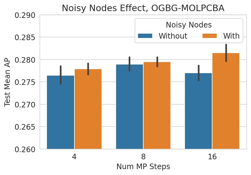
Figure 4: Adding Noisy Nodes with random flipping of input categories improves the performance of MPNNs, and the effect is accentuated with depth.

Figure 5: Validation curve comparing with and without noisy nodes. Using Noisy Nodes leads to a consistent improvement.

7.3 OGBN-ARXIV

The above results use models with explicit edge updates, and are reported for graph prediction. To test the effectiveness with Noisy Nodes with GCNs, arguably the simplest and most popular GNN, we use OGBN-ARXIV, a citation network with the goal of predicting the arxiv category of each paper. Adding Noisy Nodes, with noise as input dropout of 0.1, to 4 layer GCN with residual connections improves from 72.39% $\pm$ 0.002 accuracy to 72.52% $\pm$ 0.003 accuracy. A baseline 4 layer GCN on this dataset reports 71.71% $\pm$ 0.002. The SOTA for this dataset is 74.31% (Sun & Wu, 2020).

7.4 Limitations

We have not demonstrated the effectiveness of Noisy Nodes in small data regimes, which may be important for learning from experimental data. The representation learning perspective requires access to a local minimum configuration, which is not the case for all quantum modeling datasets. We have also not demonstrated the combination of Noisy Nodes with more sophisticated 3D molecular property prediction models such as DimeNet++(Klicpera et al., 2020a), such models may require an alternative reconstruction loss to position change, such as pairwise interatomic distances. We leave this to future work.

Noisy Nodes requires careful selection of the form of noise, and a balance between the auxiliary and primary losses. This can require hyper parameter tuning, and models can be sensitive to the choice of these parameters. Noisy Nodes has a particular effect for deep GNNs, but depth is not always an advantage. There are situations, for example molecular dynamics, which place a premium on very fast inference time. However even at 3 layers (a comparable depth to alternative architectures) the GNS architecture achieves state of the art validation OC20 IS2RE predictions (Figure 3). Finally, returns diminish as depth increases indicating depth is not the only answer (Table 1).

8 Conclusions

In this work we present Noisy Nodes, a novel regularisation technique for GNNs with particular focus on 3D molecular property prediction. Noisy nodes helps address common challenges around oversmoothed node representations, shows benefits for GNNs of all depths, but in particular improves performance for deeper GNNs. We demonstrate results on challenging 3D molecular property prediction tasks, and some generic GNN benchmark datasets. We believe these results demonstrate Noisy Nodes could be a useful building block for GNNs for molecular property prediction and beyond.

9 Reproducibility statement

Code for reproducing OGB-PCQM4M results using Noisy Nodes is available on github, and was prepared as part of a leaderboard submission. https://github.com/deepmind/deepmind-research/tree/master/ogb_lsc/pcq.

We provide detailed hyper parameter settings for all our experiments in the appendix, in addition to formulae for computing the encoder and decoder stages of the GNS.

10 Ethics statement

Who may benefit from this work? Molecular property prediction with GNNs is a fast-growing area with applications across domains such as drug design, catalyst discovery, synthetic biology, and chemical engineering. Noisy Nodes could aid models applied to these domains. We also demonstrate on OC20 that our direct state prediction approach is nearly as accurate as learned relaxed approaches at a small fraction of the computational cost, which may support material design which requires many predictions.

Finally, Noisy Nodes could be adapted and applied to many areas in which GNNs are used—for example, knowledge base completion, physical simulation or traffic prediction.

Potential negative impact and reflection. Noisy Nodes sees improved performance from depth, but the training of very deep GNNs could contribute to global warming. Care should be taken when utilising depth, and we note that Noisy Nodes settings can be calibrated at shallow depth.

Appendix A Appendix

The following sections include details on training setup, hyper-parameters, input processing, as well as additional experimental results.

A.1 Additional Metrics for Open Catalyst IS2RS Test Set

Relaxation approaches to IS2RS minimise forces with respect to positions, with the expectation that forces at the minimum are close to zero. One metric of such a model’s success is to evaluate the forces at the converged structure using ground truth Density Functional Theory calculations and see how close they are to zero. Two metrics are provided by OC20 (Chanussot* et al., 2020) on the IS2RS test set: Force below Threshold (FbT), which is the percentage of structures that have forces below 0.05 eV/Angstrom, and Average Force below Threshold (AFbT) which is FbT calculated at multiple thresholds.

The OC20 project computes test DFT calculations on the evaluation server and presents a summary result for all IS2RS position predictions. Such calculations take 10-12 hours and they are not available for the validation set. Thus, we are not able to analyse the results in Tables 8 and 9 in any further detail. Before application to catalyst screening further work may be needed for direct approaches to ensure forces do not explode from atoms being too close together.

Table 8: OC20 IS2RS Test, Average Force below Threshold %, $\uparrow$

Model	Method	OOD Both	OOD Adsorbate	OOD Catalyst	ID
Noisy Nodes	Direct	0.09%	0.00%	0.29%	0.54%

Table 9: OC20 IS2RS Test, Force below Threshold %, $\uparrow$

Model	Method	OOD Both	OOD Adsorbate	OOD Catalyst	ID
Noisy Nodes	Direct	0.0%	0.0%	0.0%	0.0%

A.2 More details on GNS adaptations for molecular property prediction.

Encoder.

The node features are a learned embedding lookup of the atom type, and in the case of OC20 two additional binary features representing whether the atom is part of the adsorbate or catalyst and whether the atom remains fixed during the quantum chemistry simulation.

The edge features, $e_{k}$ are the distances $|d|$ featurised using $c$ Radial Bessel basis functions, $\tilde{e}_{RBF,c}=\sqrt{\frac{2}{R}}\frac{\text{sin}(\frac{c\pi}{R}d)}{d}$, and the edge vector displacements, $d$, normalised by the edge distance:

$$e_{k}=\text{Concat}(\tilde{e}_{RBF,1}(|d|),\text{...},\tilde{e}_{RBF,c}(|d|),\frac{d}{|d|})$$

Our conversion to fractional coordinates only applied to the vector quantities, i.e. $\frac{d}{|d|}$.

Decoder

The decoder consists of two parts, a graph-level decoder which predicts a single output for the input graph, and a node-level decoder which predicts individual outputs for each node. The graph-level decoder implements the following equation:

$$y=W^{\text{Proc}}\sum_{i=1}^{|V|}\text{MLP}_{\text{Proc}}(a_{i}^{\text{Proc}})+b^{\text{Proc}}+W^{\text{Enc}}\sum_{i=1}^{|V|}\text{MLP}_{\text{Enc}}(a_{i}^{\text{Enc}})+b^{\text{Enc}}$$

Where $a_{i}^{\text{Proc}}$ are node latents from the Processor, $a_{i}^{\text{Enc}}$ are node latents from the Encoder, $W^{\text{Enc}}$ and $W^{\text{Proc}}$ are linear layers, $b^{\text{Enc}}$ and $b^{\text{Proc}}$ are biases, and $|V|$ is the number of nodes. The node-level decoder is simply an MLP applied to each $a_{i}^{\text{Proc}}$ which predicts $a_{i}^{\Delta}$.

A.3 More details on MPNN for OGBG-PCQM4M and OGBG-MOLPCBA

Our MPNN follows the blueprint of Gilmer et al. (2017). We use $\vec{h}^{(t)}_{v}$ to denote the latent vector of node $v$ at message passing step $t$, and $\vec{m}^{(t)}_{uv}$ to be the computed message vector for the edge between nodes $u$ and $v$ at message passing step $t$. We define the update functions as:

$$\vec{m}^{(t+1)}_{uv} =\psi_{t+1}\left(\vec{h}^{(t)}_{u},\vec{h}^{(t)}_{v},\vec{m}^{(t)}_{uv}+\vec{m}^{(t-1)}_{uv}\right)$$ (1)

$$\vec{h}^{(t+1)}_{u} =\phi_{t+1}\left(\vec{h}^{(t)}_{u},\sum_{u\in\mathcal{N}_{v}}\vec{m}^{(t+1)}_{vu},\sum_{v\in\mathcal{N}_{u}}\vec{m}^{(t+1)}_{uv}\right)+\vec{h}^{t}_{u}$$ (2)

Where the message function $\psi_{t+1}$ and the update function $\phi_{t+1}$ are MLPs. We use a “Virtual Node” which is connected to all other nodes to enable long range communication. Out readout function is an MLP. No spatial features are used.

A.4 Experiment setup for 3D Molecular Modeling

Open Catalyst. All training experiments were ran on a cluster of TPU devices. For the Open Catalyst experiments, each individual run (i.e. a single random seed) utilised 8 TPU devices on 2 hosts (4 per host) for training, and 4 V100 GPU devices for evaluation (1 per dataset).

Each Open Catalyst experiment was ran until convergence for up to 200 hours. Our best result, the large 100 layer model requires 7 days of training using the above setting. Each configuration was run at least 3 times in this hardware configuration, including all ablation settings.

We further note that making effective use of our regulariser requires sweeping noise values. These sweeps are dataset dependent and can be carried out using few message passing steps.

QM9. Experiments were also run on TPU devices. Each seed was run using 8 TPU devices on a single host for training, and 2 V100 GPU devices for evaluation. QM9 targets were trained between 12-24 hours per experiment.

Following Klicpera et al. (2020b) we define std. MAE as :

$$\text{std. MAE}=\frac{1}{M}\sum^{M}_{m=1}\left(\frac{1}{N}\sum^{N}_{i=1}\frac{|f_{\theta}^{(m)}(\bm{X}_{i},\bm{z}_{i})-\hat{t}_{i}^{(m)}|}{\sigma_{m}}\right)$$

and logMAE as:

$$\text{logMAE}=\frac{1}{M}\sum^{M}_{m=1}\text{log}\left(\frac{1}{N}\sum^{N}_{i=1}\frac{|f_{\theta}^{(m)}(\bm{X}_{i},\bm{z}_{i})-\hat{t}_{i}^{(m)}|}{\sigma_{m}}\right)$$

with target index $m$, number of targets $M=12$, dataset size $N$, ground truth values $\hat{t}^{(m)}$, model $f_{\theta}^{(m)}$, inputs $\bm{X}_{i}$ and $z_{i}$, and standard deviation $\sigma_{m}$ of $\hat{t}^{(m)}$.

A.5 Over Smoothing Analysis for GNS

In addition to Figure 2, we repeat the analysis with a mean MAD over 3 seeds 7. Furthermore we remove the sorting layer by MAD value and find the trend holds.

Figure 6: GNS Unsorted MAD per Layer Averaged Over 3 Random Seeds. Evidence of oversmoothing is clear. Model trained on QM9.

Figure 7: GNS Sorted MAD per Layer Averaged Over 3 Random Seeds. The trend is clearer when the MAD values have been sorted. Model trained on QM9.

A.6 Noise Ablations for OGBG-MOLPCBA

We conduct a noise ablation on the random flipping noise for OGBG-MOLPCBA with an 8 layer MPNN + Virtual Node, and find that our model is not very sensitive to the noise value (Table 10), but degrades from 0.1.

Flip Probability	Mean AP
0.01	27.8% +- 0.002
0.03	27.9% +- 0.003
0.05	$\bm{28.1}\%$ +- 0.001
0.1	28.0% +- 0.003
0.2	27.7% +- 0.002

Table 10: OGBG-MOLPCBA Noise Ablation

A.7 DropEdge & DropNode Ablations for OGBG-MOLPCBA

We conduct an ablation with our 16 layer MPNN using DropEdge at a rate of 0.1 as an alternative approach to improving oversmoothing and find it does not improve performance for ogbg-molpcba (Table 11), similarly we find DropNode (Table 12) does not improve performance. In addition, we find that these two methods can’t be combined well together, reaching a performance of 27.0% $\pm$ 0.003. However, both methods can be combined advantageously with Noisy Nodes.

	Mean AP
MPNN Without DropEdge	27.4% $\pm$ 0.002
MPNN With DropEdge	27.5% $\pm$ 0.001
MPNN + DropEdge + Noisy Nodes	$\bm{27.8\%}$ $\pm$ 0.002

Table 11: OGBG-MOLPCBA DropEdge Ablation

	Mean AP
MPNN With DropNode	27.5% $\pm$ 0.001
MPNN Without DropNode	27.5% $\pm$ 0.004
MPNN + DropNode + Noisy Nodes	$\bm{28.2\%}$ $\pm$ 0.005

Table 12: OGBG-MOLPCBA DropNode Ablation

We also measure the MAD of the node latents for each layer and find the indeed Noisy Nodes is more effective at addressing oversmoothing in Figure 8.

Figure 8: Comparison of the effect of techniques to address oversmoothing on MPNNs. Whilst Some effect can be seen from DropEdge and DropNode, Noisy Nodes is significantly better at preserving per node diversity.

A.8 Training Curves for OC20 Noisy Nodes Ablations Demonstrating Overfitting

Figure 9

Figure 9: Training curves to accompany Figure 3. This demonstrates that even as the validation performance is getting worse, training loss is going down, indicating overfitting.

A.9 Pseudocode for 3D Molecular Prediction Training Step

$G$ = $(V,E,g)$ // Input graph

$\tilde{G}=G$ // Initialize noisy graph

$\lambda$ // Noisy Nodes Weight

if not_provided($V^{\prime}$) then

       $V^{\prime}\leftarrow V$

end if

if predict_differences then

       $\Delta$ = $\{v^{\prime}_{i}-v_{i}|i\in 1,\dots,|V|\}$

end if

for each  $i\in 1,\dots,|V|$ do

       $\sigma_{i}$ = sample_node_noise(shape_of($v_{i}$));

       $\tilde{v}_{i}$ = $v_{i}+\sigma_{i}$;

       if predict_differences then

             $\tilde{\Delta}_{i}$ = $\Delta_{i}-\sigma_{i}$;

            

       end if

      

endfor

$\tilde{E}$ = recompute_edges($\tilde{V}$);

$\hat{G}^{\prime}$ = GNN($\tilde{G}$);

if predict_differences then

       $V^{\prime}=\tilde{\Delta}_{i}$;

      

end if

Loss = $\lambda$ NoisyNodesLoss($\hat{G}^{\prime}$, $V^{\prime}$) + PrimaryLoss($\hat{G}^{\prime}$, $V^{\prime}$));

Loss.minimise()

Algorithm 1 Noisy Nodes Training Step

A.10 Training Details

Our code base is implemented in JAX using Haiku and Jraph for GNNs, and Optax for training (Bradbury et al., 2018; Babuschkin et al., 2020; Godwin* et al., 2020; Hennigan et al., 2020). Model selection used early stopping.

All results reported as an average of 10 random seeds. OGBG-PCQM4M & OGBG-MOLPCBA were trained with 16 TPUs and evaluated with a single V100 GPU. OGBN-Arxiv was trained and evalated with a single TPU

3D Molecular Prediction

We minimise the mean squared error loss on mean and standard deviation normalised targets and use the Adam (Kingma & Ba, 2015) optimiser with warmup and cosine decay. For OC20 IS2RE energy prediction we subtract a learned reference energy, computed using an MLP with atom types as input.

For the GNS model the node and edge latents as well as MLP hidden layers were sized 512, with 3 layers per MLP and using shifted softplus activations throughout. OC20 & QM9 Models were trained on 8 TPU devices and evaluated on a single V100 GPUs. We provide the full set of hyper-parameters and computational resources used separately for each dataset in the Appendix. All noise levels were determined by sweeping a small range of values ($\approx 10$) informed by the noised feature covariance.

Non Spatial Tasks

A.11 Hyper-parameters

Open Catalyst. We list the hyper-parameters used to train the default Open Catalyst experiment. If not specified otherwise (e.g. in ablations of these parameters), experiments were ran with this configuration.

Table 13: Open Catalyst training parameters.

Parameter	Value or description
Optimiser	Adam with warm up and cosine cycling
$\beta_{1}$	$0.9$
$\beta_{2}$	$0.95$
Warm up steps	$5e5$
Warm up start learning rate	$1e-5$
Warm up/cosine max learning rate	$1e-4$
Cosine cycle length	$5e6$
Loss type	Mean squared error
Batch size	Dynamic to max edge/node/graph count
Max nodes in batch	1024
Max edges in batch	12800
Max graphs in batch	10
MLP number of layers	3
MLP hidden sizes	512
Number Bessel Functions	512
Activation	shifted softplus
message passing layers	50
Group size	10
Node/Edge latent vector sizes	512
Position noise	Gaussian ($\mu=0,\sigma=0.3$)
Parameter update	Exponentially moving average (EMA) smoothing
EMA decay	0.9999
Position Loss Co-efficient	1.0

Dynamic batch sizes refers to constructing batches by specifying maximum node, edge and graph counts (as opposed to only graph counts) to better balance computational load. Batches are constructed until one of the limits is reached.

Parameter updates were smoothed using an EMA for the current training step with the current decay value computed through $decay=min(decay,(1.0+step)/(10.0+step)$. As discussed in the evaluation, best results on Open Catalyst were obtained by utilising a 100 layer network with group size 10.

QM9 Table 14 lists QM9 hyper-parameters which primarily reflect the smaller dataset and geometries with fewer long range interactions. For $U_{0}$, $U$, $H$ and $G$ we use a slightly larger number of graphs per batch - 16 - and a smaller position loss co-efficient of 0.01.

Table 14: QM9 training parameters.

Parameter	Value or description
Optimiser	Adam with warm up and cosine cycling
$\beta_{1}$	$0.9$
$\beta_{2}$	$0.95$
Warm up steps	$1e4$
Warm up start learning rate	$3e-7$
Warm up/cosine max learning rate	$1e-4$
Cosine cycle length	$2e6$
Loss type	Mean squared error
Batch size	Dynamic to max edge/node/graph count
Max nodes in batch	256
Max edges in batch	4096
Max graphs in batch	8
MLP number of layers	3
MLP hidden sizes	1024
Number Bessel Funtions	512
Activation	shifted softplus
message passing layers	10
Group Size	10
Node/Edge latent vector sizes	512
Position noise	Gaussian ($\mu=0,\sigma=0.02$)
Parameter update	Exponentially moving average (EMA) smoothing
EMA decay	0.9999
Position Loss Coefficient	0.1

OGBG-PCQM4M Table 15 provides the hyper parameters for OGBG-PCQM4M.

Table 15: OGBG-PCQM4M Training Parameters.

Parameter	Value or description
Optimiser	Adam with warm up and cosine cycling
$\beta_{1}$	$0.9$
$\beta_{2}$	$0.95$
Warm up steps	$5e4$
Warm up start learning rate	$1e-5$
Warm up/cosine max learning rate	$1e-4$
Cosine cycle length	$5e5$
Loss type	Mean absolute error
Reconstruction type	Softmax Cross Entropy
Batch size	Dynamic to max edge/node/graph count
Max nodes in batch	20,480
Max edges in batch	8,192
Max graphs in batch	512
MLP number of layers	2
MLP hidden sizes	512
Activation	relu
Node/Edge latent vector sizes	512
Noisy Nodes Category Flip Fate	0.05
Parameter update	Exponentially moving average (EMA) smoothing
EMA decay	0.999
Reconstruction Loss Coefficient	0.1

OGBG-MOLPCBA Table 16 provides the hyper parameters for the OGBG-MOLPCBA experiments.

Table 16: OGBG-MOLPCBA Training Parameters.

Parameter	Value or description
Optimiser	Adam with warm up and cosine cycling
$\beta_{1}$	$0.9$
$\beta_{2}$	$0.95$
Warm up steps	$1e4$
Warm up start learning rate	$1e-5$
Warm up/cosine max learning rate	$1e-4$
Cosine cycle length	$1e5$
Loss type	Softmax Cross Entropy
Reconstruction loss type	Softmax Cross Entropy
Batch size	Dynamic to max edge/node/graph count
Max nodes in batch	20,480
Max edges in batch	8,192
Max graphs in batch	512
MLP number of layers	2
MLP hidden sizes	512
Activation	relu
Batch Normalization	Yes, after every hidden layer
Node/Edge latent vector sizes	512
Dropnode Rate	0.1
Dropout Rate	0.1
Noisy Nodes Category Flip Fate	0.05
Parameter update	Exponentially moving average (EMA) smoothing
EMA decay	0.999
Reconstruction Loss Coefficient	0.1

OGBN-ARXIV Table 17 provides the hyper parameters for the OGBN-Arxiv experiments.

Table 17: OGBG-ARXIV Training Parameters.

Parameter	Value or description
Optimiser	Adam with warm up and cosine cycling
$\beta_{1}$	$0.9$
$\beta_{2}$	$0.95$
Warm up steps	$50$
Warm up start learning rate	$1e-5$
Warm up/cosine max learning rate	$1e-3$
Cosine cycle length	$12,000$
Loss type	Softmax Cross Entropy
Reconstruction loss type	Mean Squared Error
Batch size	Full graph
MLP number of layers	1
Activation	relu
Batch Normalization	Yes, after every hidden layer
Node/Edge latent vector sizes	256
Dropout Rate	0.5
Noisy Nodes Input Dropout	0.05
Reconstruction Loss Coefficient	0.1

References

- Anderson et al. (2019) Brandon M. Anderson, T. Hy, and R. Kondor. Cormorant: Covariant molecular neural networks. In NeurIPS, 2019.
- Babuschkin et al. (2020) Igor Babuschkin, Kate Baumli, Alison Bell, Surya Bhupatiraju, Jake Bruce, Peter Buchlovsky, David Budden, Trevor Cai, Aidan Clark, Ivo Danihelka, Claudio Fantacci, Jonathan Godwin, Chris Jones, Tom Hennigan, Matteo Hessel, Steven Kapturowski, Thomas Keck, Iurii Kemaev, Michael King, Lena Martens, Vladimir Mikulik, Tamara Norman, John Quan, George Papamakarios, Roman Ring, Francisco Ruiz, Alvaro Sanchez, Rosalia Schneider, Eren Sezener, Stephen Spencer, Srivatsan Srinivasan, Wojciech Stokowiec, and Fabio Viola. The DeepMind JAX Ecosystem, 2020. URL http://github.com/deepmind.
- Bapst et al. (2020) V. Bapst, T. Keck, Agnieszka Grabska-Barwinska, C. Donner, E. D. Cubuk, S. Schoenholz, A. Obika, Alexander W. R. Nelson, T. Back, D. Hassabis, and P. Kohli. Unveiling the predictive power of static structure in glassy systems. Nature Physics, 16:448–454, 2020.
- Battaglia et al. (2018) P. Battaglia, Jessica B. Hamrick, V. Bapst, A. Sanchez-Gonzalez, V. Zambaldi, Mateusz Malinowski, Andrea Tacchetti, David Raposo, A. Santoro, R. Faulkner, Çaglar Gülçehre, H. Song, A. J. Ballard, J. Gilmer, George E. Dahl, Ashish Vaswani, Kelsey R. Allen, Charlie Nash, Victoria Langston, Chris Dyer, N. Heess, Daan Wierstra, P. Kohli, M. Botvinick, Oriol Vinyals, Y. Li, and Razvan Pascanu. Relational inductive biases, deep learning, and graph networks. ArXiv, abs/1806.01261, 2018.
- Batzner et al. (2021) Simon Batzner, T. Smidt, L. Sun, J. Mailoa, M. Kornbluth, N. Molinari, and B. Kozinsky. Se(3)-equivariant graph neural networks for data-efficient and accurate interatomic potentials. ArXiv, abs/2101.03164, 2021.
- Bishop (1995) Charles M. Bishop. Training with noise is equivalent to tikhonov regularization. Neural Computation, 7:108–116, 1995.
- Bradbury et al. (2018) James Bradbury, Roy Frostig, Peter Hawkins, Matthew James Johnson, Chris Leary, Dougal Maclaurin, George Necula, Adam Paszke, Jake VanderPlas, Skye Wanderman-Milne, and Qiao Zhang. JAX: composable transformations of Python+NumPy programs, 2018. URL http://github.com/google/jax.
- Bronstein et al. (2017) Michael M Bronstein, Joan Bruna, Yann LeCun, Arthur Szlam, and Pierre Vandergheynst. Geometric deep learning: going beyond euclidean data. IEEE Signal Processing Magazine, 34(4):18–42, 2017.
- Brown et al. (2020) T. Brown, Benjamin Mann, Nick Ryder, Melanie Subbiah, J. Kaplan, Prafulla Dhariwal, Arvind Neelakantan, Pranav Shyam, Girish Sastry, Amanda Askell, Sandhini Agarwal, Ariel Herbert-Voss, Gretchen Krueger, T. Henighan, R. Child, A. Ramesh, Daniel M. Ziegler, Jeffrey Wu, Clemens Winter, Christopher Hesse, Mark Chen, Eric Sigler, Mateusz Litwin, Scott Gray, Benjamin Chess, J. Clark, Christopher Berner, Sam McCandlish, Alec Radford, Ilya Sutskever, and Dario Amodei. Language models are few-shot learners. ArXiv, abs/2005.14165, 2020.
- Cai & Wang (2020) Chen Cai and Yusu Wang. A note on over-smoothing for graph neural networks. CoRR, abs/2006.13318, 2020. URL https://arxiv.org/abs/2006.13318.
- Chanussot* et al. (2020) Lowik Chanussot*, Abhishek Das*, Siddharth Goyal*, Thibaut Lavril*, Muhammed Shuaibi*, Morgane Riviere, Kevin Tran, Javier Heras-Domingo, Caleb Ho, Weihua Hu, Aini Palizhati, Anuroop Sriram, Brandon Wood, Junwoong Yoon, Devi Parikh, C. Lawrence Zitnick, and Zachary Ulissi. Open catalyst 2020 (oc20) dataset and community challenges. ACS Catalysis, 0(0):6059–6072, 2020. doi: 10.1021/acscatal.0c04525. URL https://doi.org/10.1021/acscatal.0c04525.
- Chen et al. (2019) Deli Chen, Yankai Lin, Wei Li, Peng Li, Jie Zhou, and Xu Sun. Measuring and relieving the over-smoothing problem for graph neural networks from the topological view. CoRR, abs/1909.03211, 2019. URL http://arxiv.org/abs/1909.03211.
- Chen et al. (2020) Deli Chen, Yankai Lin, W. Li, Peng Li, J. Zhou, and Xu Sun. Measuring and relieving the over-smoothing problem for graph neural networks from the topological view. In AAAI, 2020.
- Chmiela et al. (2017) Stefan Chmiela, A. Tkatchenko, H. E. Sauceda, I. Poltavsky, Kristof T. Schütt, and K. Müller. Machine learning of accurate energy-conserving molecular force fields. Science Advances, 3, 2017.
- Dasoulas et al. (2019) George Dasoulas, Ludovic Dos Santos, Kevin Scaman, and Aladin Virmaux. Coloring graph neural networks for node disambiguation. ArXiv, abs/1912.06058, 2019.
- Devlin et al. (2019) J. Devlin, Ming-Wei Chang, Kenton Lee, and Kristina Toutanova. Bert: Pre-training of deep bidirectional transformers for language understanding. In NAACL-HLT, 2019.
- Do et al. (2021) Tien Huu Do, Duc Minh Nguyen, Giannis Bekoulis, Adrian Munteanu, and N. Deligiannis. Graph convolutional neural networks with node transition probability-based message passing and dropnode regularization. Expert Syst. Appl., 174:114711, 2021.
- Duvenaud et al. (2015) David Duvenaud, Dougal Maclaurin, Jorge Aguilera-Iparraguirre, Rafael Gómez-Bombarelli, Timothy Hirzel, Alán Aspuru-Guzik, and Ryan P. Adams. Convolutional networks on graphs for learning molecular fingerprints. In Proceedings of the 28th International Conference on Neural Information Processing Systems - Volume 2, NIPS’15, pp. 2224–2232, Cambridge, MA, USA, 2015. MIT Press.
- Fuchs et al. (2020) F. Fuchs, Daniel E. Worrall, Volker Fischer, and M. Welling. Se(3)-transformers: 3d roto-translation equivariant attention networks. ArXiv, abs/2006.10503, 2020.
- Gilmer et al. (2017) J. Gilmer, S. Schoenholz, Patrick F. Riley, Oriol Vinyals, and George E. Dahl. Neural message passing for quantum chemistry. ArXiv, abs/1704.01212, 2017.
- Godwin* et al. (2020) Jonathan Godwin*, Thomas Keck*, Peter Battaglia, Victor Bapst, Thomas Kipf, Yujia Li, Kimberly Stachenfeld, Petar Veličković, and Alvaro Sanchez-Gonzalez. Jraph: A library for graph neural networks in jax., 2020. URL http://github.com/deepmind/jraph.
- Hennigan et al. (2020) Tom Hennigan, Trevor Cai, Tamara Norman, and Igor Babuschkin. Haiku: Sonnet for JAX, 2020. URL http://github.com/deepmind/dm-haiku.
- Hu et al. (2020a) Weihua Hu, Matthias Fey, Marinka Zitnik, Yuxiao Dong, Hongyu Ren, Bowen Liu, Michele Catasta, and Jure Leskovec. Open graph benchmark: Datasets for machine learning on graphs. ArXiv, abs/2005.00687, 2020a.
- Hu et al. (2020b) Weihua Hu, Bowen Liu, Joseph Gomes, M. Zitnik, Percy Liang, V. Pande, and J. Leskovec. Strategies for pre-training graph neural networks. arXiv: Learning, 2020b.
- Hu et al. (2021a) Weihua Hu, Matthias Fey, Hongyu Ren, Maho Nakata, Yuxiao Dong, and Jure Leskovec. Ogb-lsc: A large-scale challenge for machine learning on graphs. arXiv preprint arXiv:2103.09430, 2021a.
- Hu et al. (2021b) Weihua Hu, Muhammed Shuaibi, Abhishek Das, Siddharth Goyal, Anuroop Sriram, J. Leskovec, Devi Parikh, and C. L. Zitnick. Forcenet: A graph neural network for large-scale quantum calculations. ArXiv, abs/2103.01436, 2021b.
- Jumper et al. (2021) John M. Jumper, Richard Evans, Alexander Pritzel, Tim Green, Michael Figurnov, Olaf Ronneberger, Kathryn Tunyasuvunakool, Russ Bates, Augustin Zídek, Anna Potapenko, Alex Bridgland, Clemens Meyer, Simon A A Kohl, Andy Ballard, Andrew Cowie, Bernardino Romera-Paredes, Stanislav Nikolov, Rishub Jain, Jonas Adler, Trevor Back, Stig Petersen, David A. Reiman, Ellen Clancy, Michal Zielinski, Martin Steinegger, Michalina Pacholska, Tamas Berghammer, Sebastian Bodenstein, David Silver, Oriol Vinyals, Andrew W. Senior, Koray Kavukcuoglu, Pushmeet Kohli, and Demis Hassabis. Highly accurate protein structure prediction with alphafold. Nature, 596:583 – 589, 2021.
- Kingma & Ba (2015) Diederik P. Kingma and Jimmy Ba. Adam: A method for stochastic optimization. CoRR, abs/1412.6980, 2015.
- Kipf & Welling (2016) Thomas N. Kipf and Max Welling. Semi-supervised classification with graph convolutional networks. CoRR, abs/1609.02907, 2016. URL http://arxiv.org/abs/1609.02907.
- Klicpera et al. (2020a) Johannes Klicpera, Shankari Giri, Johannes T. Margraf, and Stephan Günnemann. Fast and uncertainty-aware directional message passing for non-equilibrium molecules. CoRR, abs/2011.14115, 2020a. URL https://arxiv.org/abs/2011.14115.
- Klicpera et al. (2020b) Johannes Klicpera, Janek Groß, and Stephan Günnemann. Directional message passing for molecular graphs. ArXiv, abs/2003.03123, 2020b.
- Kondor et al. (2018) Risi Kondor, Hy Truong Son, Horace Pan, Brandon M. Anderson, and Shubhendu Trivedi. Covariant compositional networks for learning graphs. CoRR, abs/1801.02144, 2018. URL http://arxiv.org/abs/1801.02144.
- Kong et al. (2020) Kezhi Kong, Guohao Li, Mucong Ding, Zuxuan Wu, Chen Zhu, Bernard Ghanem, G. Taylor, and T. Goldstein. Flag: Adversarial data augmentation for graph neural networks. ArXiv, abs/2010.09891, 2020.
- Köhler et al. (2019) Jonas Köhler, Leon Klein, and Frank Noé. Equivariant flows: sampling configurations for multi-body systems with symmetric energies, 2019.
- Li et al. (2019) G. Li, M. Müller, Ali K. Thabet, and Bernard Ghanem. Deepgcns: Can gcns go as deep as cnns? 2019 IEEE/CVF International Conference on Computer Vision (ICCV), pp. 9266–9275, 2019.
- Li et al. (2020) Guohao Li, C. Xiong, Ali K. Thabet, and Bernard Ghanem. Deepergcn: All you need to train deeper gcns. ArXiv, abs/2006.07739, 2020.
- Li et al. (2021) Guohao Li, Matthias Müller, Bernard Ghanem, and Vladlen Koltun. Training graph neural networks with 1000 layers. CoRR, abs/2106.07476, 2021. URL https://arxiv.org/abs/2106.07476.
- Li et al. (2018) Qimai Li, Zhichao Han, and Xiao-Ming Wu. Deeper insights into graph convolutional networks for semi-supervised learning. In Proceedings of the AAAI Conference on Artificial Intelligence, volume 32, 2018.
- Liu et al. (2021) Yi Liu, Limei Wang, Meng Liu, Xuan Zhang, Bora Oztekin, and Shuiwang Ji. Spherical message passing for 3d graph networks. arXiv preprint arXiv:2102.05013, 2021.
- Loukas (2020) Andreas Loukas. How hard is to distinguish graphs with graph neural networks? arXiv: Learning, 2020.
- Murphy et al. (2019) Ryan L. Murphy, Balasubramaniam Srinivasan, Vinayak A. Rao, and Bruno Ribeiro. Relational pooling for graph representations. In ICML, 2019.
- Pfaff et al. (2020) T. Pfaff, Meire Fortunato, Alvaro Sanchez-Gonzalez, and P. Battaglia. Learning mesh-based simulation with graph networks. ArXiv, abs/2010.03409, 2020.
- Ramakrishnan et al. (2014) R. Ramakrishnan, Pavlo O. Dral, M. Rupp, and O. A. von Lilienfeld. Quantum chemistry structures and properties of 134 kilo molecules. Scientific Data, 1, 2014.
- Rong et al. (2019) Yu Rong, Wenbing Huang, Tingyang Xu, and Junzhou Huang. The truly deep graph convolutional networks for node classification. CoRR, abs/1907.10903, 2019. URL http://arxiv.org/abs/1907.10903.
- Sanchez-Gonzalez et al. (2018) Alvaro Sanchez-Gonzalez, N. Heess, Jost Tobias Springenberg, J. Merel, Martin A. Riedmiller, R. Hadsell, and P. Battaglia. Graph networks as learnable physics engines for inference and control. ArXiv, abs/1806.01242, 2018.
- Sanchez-Gonzalez* et al. (2020) Alvaro Sanchez-Gonzalez*, Jonathan Godwin*, Tobias Pfaff*, Rex Ying*, Jure Leskovec, and Peter Battaglia. Learning to simulate complex physics with graph networks. In Hal Daumé III and Aarti Singh (eds.), Proceedings of the 37th International Conference on Machine Learning, volume 119 of Proceedings of Machine Learning Research, pp. 8459–8468. PMLR, 13–18 Jul 2020. URL http://proceedings.mlr.press/v119/sanchez-gonzalez20a.html.
- Sato et al. (2021) R. Sato, Makoto Yamada, and Hisashi Kashima. Random features strengthen graph neural networks. In SDM, 2021.
- Satorras et al. (2021) Victor Garcia Satorras, Emiel Hoogeboom, and Max Welling. E(n) equivariant graph neural networks, 2021.
- Scarselli et al. (2009) Franco Scarselli, Marco Gori, Ah Chung Tsoi, Markus Hagenbuchner, and Gabriele Monfardini. The graph neural network model. IEEE Transactions on Neural Networks, 20(1):61–80, 2009. doi: 10.1109/TNN.2008.2005605.
- Schütt et al. (2017) Kristof Schütt, Pieter-Jan Kindermans, Huziel Enoc Sauceda Felix, Stefan Chmiela, A. Tkatchenko, and K. Müller. Schnet: A continuous-filter convolutional neural network for modeling quantum interactions. In NIPS, 2017.
- Shlomi et al. (2021) Jonathan Shlomi, Peter Battaglia, and Jean-Roch Vlimant. Graph neural networks in particle physics. Machine Learning: Science and Technology, 2(2):021001, Jan 2021. ISSN 2632-2153. doi: 10.1088/2632-2153/abbf9a. URL http://dx.doi.org/10.1088/2632-2153/abbf9a.
- Sietsma & Dow (1991) J. Sietsma and Robert J. F. Dow. Creating artificial neural networks that generalize. Neural Networks, 4:67–79, 1991.
- Song & Ermon (2019) Yang Song and Stefano Ermon. Generative modeling by estimating gradients of the data distribution. ArXiv, abs/1907.05600, 2019.
- Sun & Wu (2020) Chuxiong Sun and Guoshi Wu. Adaptive graph diffusion networks with hop-wise attention. ArXiv, abs/2012.15024, 2020.
- Thakoor et al. (2021) Shantanu Thakoor, C. Tallec, M. G. Azar, R. Munos, Petar Velivckovi’c, and Michal Valko. Bootstrapped representation learning on graphs. ArXiv, abs/2102.06514, 2021.
- Thomas et al. (2018) Nathaniel Thomas, Tess Smidt, Steven M. Kearnes, Lusann Yang, Li Li, Kai Kohlhoff, and Patrick Riley. Tensor field networks: Rotation- and translation-equivariant neural networks for 3d point clouds. CoRR, abs/1802.08219, 2018. URL http://arxiv.org/abs/1802.08219.
- Unke & Meuwly (2019) Oliver T. Unke and Markus Meuwly. Physnet: A neural network for predicting energies, forces, dipole moments, and partial charges. Journal of Chemical Theory and Computation, 15(6):3678–3693, May 2019. ISSN 1549-9626. doi: 10.1021/acs.jctc.9b00181. URL http://dx.doi.org/10.1021/acs.jctc.9b00181.
- Vaswani et al. (2017) Ashish Vaswani, Noam M. Shazeer, Niki Parmar, Jakob Uszkoreit, Llion Jones, Aidan N. Gomez, Lukasz Kaiser, and Illia Polosukhin. Attention is all you need. ArXiv, abs/1706.03762, 2017.
- Veličković et al. (2018) Petar Veličković, Guillem Cucurull, Arantxa Casanova, Adriana Romero, Pietro Liò, and Yoshua Bengio. Graph attention networks, 2018.
- Vignac et al. (2020) Cl’ement Vignac, Andreas Loukas, and Pascal Frossard. Building powerful and equivariant graph neural networks with structural message-passing. arXiv: Learning, 2020.
- Vincent (2011) Pascal Vincent. A connection between score matching and denoising autoencoders. Neural Computation, 23:1661–1674, 2011.
- Vincent et al. (2008) Pascal Vincent, H. Larochelle, Yoshua Bengio, and Pierre-Antoine Manzagol. Extracting and composing robust features with denoising autoencoders. In ICML ’08, 2008.
- Vincent et al. (2010) Pascal Vincent, H. Larochelle, Isabelle Lajoie, Yoshua Bengio, and Pierre-Antoine Manzagol. Stacked denoising autoencoders: Learning useful representations in a deep network with a local denoising criterion. J. Mach. Learn. Res., 11:3371–3408, 2010.
- Wu et al. (2020) Zonghan Wu, Shirui Pan, Fengwen Chen, Guodong Long, Chengqi Zhang, and S Yu Philip. A comprehensive survey on graph neural networks. IEEE transactions on neural networks and learning systems, 2020.
- Xu et al. (2018) Keyulu Xu, Weihua Hu, Jure Leskovec, and Stefanie Jegelka. How powerful are graph neural networks? CoRR, abs/1810.00826, 2018. URL http://arxiv.org/abs/1810.00826.
- Yang et al. (2020) Chaoqi Yang, Ruijie Wang, Shuochao Yao, Shengzhong Liu, and Tarek Abdelzaher. Revisiting" over-smoothing" in deep gcns. arXiv preprint arXiv:2003.13663, 2020.
- Ying et al. (2021) Chengxuan Ying, Tianle Cai, Shengjie Luo, Shuxin Zheng, Guolin Ke, Di He, Yanming Shen, and Tie-Yan Liu. Do transformers really perform bad for graph representation? ArXiv, abs/2106.05234, 2021.
- You et al. (2020) Yuning You, Tianlong Chen, Yongduo Sui, Ting Chen, Zhangyang Wang, and Yang Shen. Graph contrastive learning with augmentations. ArXiv, abs/2010.13902, 2020.
- Zhao & Akoglu (2020) L. Zhao and Leman Akoglu. Pairnorm: Tackling oversmoothing in gnns. ArXiv, abs/1909.12223, 2020.
- Zhou et al. (2020a) Jie Zhou, Ganqu Cui, Shengding Hu, Zhengyan Zhang, Cheng Yang, Zhiyuan Liu, Lifeng Wang, Changcheng Li, and Maosong Sun. Graph neural networks: A review of methods and applications. AI Open, 1:57–81, 2020a.
- Zhou et al. (2020b) Kuangqi Zhou, Yanfei Dong, Wee Sun Lee, Bryan Hooi, Huan Xu, and Jiashi Feng. Effective training strategies for deep graph neural networks. CoRR, abs/2006.07107, 2020b. URL https://arxiv.org/abs/2006.07107.