Electric conductivity with the magnetic field and the chiral anomaly
in a holographic QCD model

Abstract

We calculate the electric conductivity $\sigma$ in deconfined QCD matter using a holographic QCD model, i.e., the Sakai-Sugimoto Model with varying magnetic field $B$ and chiral anomaly strength. After confirming that our estimated $\sigma$ for $B=0$ is consistent with the lattice-QCD results, we study the case with $B\neq 0$ in which the coefficient $\alpha$ in the Chern-Simons term controls the chiral anomaly strength. Our results imply that the transverse conductivity, $\sigma_{\perp}$, is suppressed to be $\lesssim 70\%$ at $B\sim 1\,\text{GeV}^{2}$ as compared to the $B=0$ case when the temperature is fixed as $T=0.2\,\text{GeV}$. Since the Sakai-Sugimoto Model has massless fermions, the longitudinal conductivity, $\sigma_{\parallel}$, with $B\neq 0$ should diverge due to production of the matter chirality. Yet, it is possible to extract a regulated part out from $\sigma_{\parallel}$ with an extra condition to neutralize the matter chirality. This regulated quantity is interpreted as an Ohmic part of $\sigma_{\parallel}$. We show that the longitudinal Ohmic conductivity increases with increasing $B$ for small $\alpha$, while it is suppressed with larger $B$ for physical $\alpha=3/4$ due to anomaly induced interactions.

I Introduction

Chiral anomaly has been a profitable probe to the nonperturbative sector of quantum field theories such as quantum chromodynamics (QCD) since its discovery dated back in the ’60s Bell and Jackiw (1969); *Adler:1969gk. The resolution of the PCAC (partially conserved axial current) puzzle Sutherland (1967) via anomalous $\pi^{0}\to\gamma\gamma$ is the most well known example. The virtue of the chiral anomaly is not limited to a specific calculation of the decay rate, and the chiral anomaly has gone on to manifest itself in various QCD phenomena. Another famous example is the $\eta$-$\eta^{\prime}$ puzzle or the $\mathrm{U(1)_{A}}$ puzzle; that is, the $\eta^{\prime}$ mass is significantly heavier than other pseudo scalar mesons belonging to the same nonet. It was ’t Hooft who gave the explanation by the instanton mechanism ’t Hooft (1976) associated with the chiral anomaly. A more recent example is found in discussions on the QCD phase diagram and a hypothetical critical point may emerge from the quark-quark and quark-antiquark coupling induced by the chiral anomaly Hatsuda et al. (2006); *Abuki:2010jq. We should emphasize that the chiral anomaly exists not only in QCD but in a wider class of gauge theories with chiral fermions. The establishment of three dimensional materials with relativistic fermionic dispersions, namely, the Weyl semimetals and the Dirac semimetals, has expanded the relevance of the chiral anomaly to physics of condensed matter.

In QCD it has been a longstanding problem how to reveal topologically nontrivial aspects of the QCD vacuum experimentally, though we are theoretically familiar with the QCD vacuum structure well; for example, Dashen’s phenomenon Dashen (1971) is textbook knowledge but there is no way to verify it by nuclear experiments. Along these lines the Chiral Magnetic Effect (CME) has been proposed as an experimental signature of the chiral anomaly detected in nuclear experiments Kharzeev et al. (2008), which was formulated in terms of the chiral chemical potential $\mu_{5}$ field-theoretically later Fukushima et al. (2008). The CME predicts anomalous generation of the electric current in parallel to an applied magnetic field $B$ (see Ref. Gursoy et al. (2014) for magnetic effects in the heavy-ion collision experiments) if a medium has imbalanced chirality; see also Refs. Miransky and Shovkovy (2015); Fukushima (2019) for reviews on nontrivial magnetic field effects. Interestingly, the electric current is anomaly protected and not renormalized with interactions, which also indicates that the current is nondissipative. We can understand this nondissipative nature from the fact that the coefficient in response to $B$ is $T$ even, making a sharp contrast to the Ohmic conductivity which is $T$ odd since the electric field $E$ has the time reversal property opposite to $B$. Interested readers can consult a comprehensive review Kharzeev et al. (2016) for theoretical backgrounds and experimental prospects of the CME and related chiral effects such as the Chiral Separation Effect, the Chiral Vortical Effect, etc (see also Ref. Kharzeev and Liao (2021) for the ongoing projects of the nuclear experiments).

It was an ingenious idea that the electric conductivity could exhibit characteristic dependence on the magnetic field to signify the CME: the longitudinal electric conductivity, $\sigma_{\parallel}$, involves chirality production due to parallel $E$ and $B$ and the produced chirality gives rise to the CME in response to $B$ again. Thus, in total, $\sigma_{\parallel}$ is expected to have a CME induced contribution that increases as $\propto B^{2}$. This increasing behavior of $\sigma_{\parallel}\propto B^{2}$ (i.e., the decreasing behavior of the resistance $\sim\sigma_{\parallel}^{-1}\propto B^{-2}$) is referred to as the negative magnetoresistance Son and Spivak (2013). In fact, in condensed matter systems, the negative magnetoresistance has been observed and it is believed that the CME has an experimental confirmation, as first reported in Ref. Li et al. (2016), but there are two major gaps between theory and experiment.

First, for undoubted establishment, it is crucial to make reliable theory estimates for the anomaly related $\sigma_{\parallel}$. In both Refs. Son and Spivak (2013); Li et al. (2016) the relaxation time approximation was employed with a strong assumption that the relaxation time is $B$ independent. In principle fermion interactions at the microscopic level may have significant $B$ dependence which may in turn change the $B$ dependence of $\sigma_{\parallel}$. Theoretical studies hitherto only concentrated on extreme regions of the parameters. In the strong magnetic field regime at high enough temperature $T$, perturbative QCD calculations become feasible in the lowest Landau level (LLL) approximation Hattori and Satow (2016); *Hattori:2016lqx. This LLL approximation was relaxed later and the full Landau level sum was taken in Ref. Fukushima and Hidaka (2018); *Fukushima:2019ugr. However, high $T$ is still required to justify the weak coupling treatment. In QCD the asymptotic freedom guarantees the validity of the weak coupling treatment at high $T$, but the condensed matter system may not have such a property. We therefore need to gain some insights into nonperturbative computations.

Second, it would be indispensable to quantify the $B$ dependence in other pieces of the electric conductivity. Because the fermion interactions are generally affected by $B$, even without the chiral anomaly, the Ohmic part of $\sigma_{\parallel}$ should be $B$ dependent. If its dependence looks similar to what is expected from the chiral anomaly, the physical interpretation of the negative magnetoresistance would become subtle. We should then discuss not only whether the $B$ dependence is positive or negative, but we must go through quantitative comparisons. Besides, it is anyway an interesting theory question how the Ohmic $\sigma_{\parallel}$ may be changed by the chiral anomaly. If the chirality production process is discarded (which will be discussed in this work), no CME contribution of $\sigma_{\parallel}\propto B^{2}$ arises, but still a finite Ohmic part can be sensitive to the strength of the chiral anomaly. One might think that the anomaly is dictated by the theory and it is unrealistic to control its strength. In the holographic QCD model, as we will explain soon later, we have a parameter to control it. Intuitively, this manipulation of changing the anomaly parameter is analogous to exploring the effect of the $\mathrm{U(1)_{A}}$ breaking interaction in QCD, i.e., the Kobayashi-Maskawa-’t Hooft interaction in chiral effective models. For example, the fate of the QCD Critical Point may differ depending on how much the effective restoration of $\mathrm{U(1)_{A}}$ symmetry occurs Fukushima (2008); *Chen:2009gv. The point is that the axial Ward identity itself is intact, but its expectation value could be changed by the instanton density accommodated by the considered state Shuryak (1994). In principle it should arise from systematic calculations, but we will use a probe approximation in which back reactions are dropped. In this approximation we do not know how much the chirality production would be affected by medium effects, and we will emulate such effects by modifying a control parameter.

For our present purpose to resolve the aforementioned problems, the Sakai-Sugimoto Model (SSM) is an advantageous choice Sakai and Sugimoto (2005a) (see Ref. Rebhan (2015) for a review for nuclear physicists, and Ref. Gürsoy (2021) for a review on holographic QCD matter at finite $B$, and also Ref. Nakas and Rigatos (2020) for a related work on the baryon operator). The SSM is one of the most established holographic QCD models and it has the same low-energy degrees of freedom as QCD. The most notable feature of the SSM is that it realizes exactly the same pattern of the chiral symmetry breaking. This model has been quite successful in reproducing the hadron spectrum as shown in the original proposal Sakai and Sugimoto (2005a), and the applications cover even the glueball physics Brünner et al. (2015); *Brunner:2015yha. In the context of the CME physics, the chiral magnetic conductivity in the presence of $\mu_{5}$ was first reproduced correctly in Ref. Yee (2009), but the treatment of $\mu_{5}$ caused some problematic complications, which was clearly pointed out in Ref. Rebhan et al. (2010). In contrast the negative magnetoresistance would not need $\mu_{5}$, and what should be calculated is the $B$ dependence of $\sigma_{\parallel}$. Interestingly, there are preceding works, Ref. Bergman et al. (2008) at $B=0$ and Ref. Lifschytz and Lippert (2009) at $B\neq 0$, for the holographic conductivity estimates in the SSM. See Ref. Li et al. (2018); Bu et al. (2019a); *Bu:2019mow for discussions in a different holographic setup. We also mention that nontrivial behavior of the magnetoresistance (including a positive value) has been found by holographic calculations in Refs. Landsteiner et al. (2015); *Jimenez-Alba:2015awa; Sun and Yang (2016). A more recent calculation of the conductivity in a Einstein-dilaton-three-Maxwell holographic model is found in Ref. Aref’eva et al. (2021). It is highly nontrivial to compare our results to preceding ones due to model and convention differences, but a solid conclusion of Ref. Lifschytz and Lippert (2009) is that the longitudinal conductivity diverges with massless fermions. This is naturally understood within the framework of the SSM; in the massless theory the produced chirality does not decay. So, the chirality charge increases proportional to the time $t$, and the CME current increases also as $\propto t$, which makes the conductivity at the zero frequency limit diverge. Thus, the divergence of the conductivity is a physically sensible behavior. It should be noted that the chirality can in principle relax even in the massless theory Iatrakis et al. (2015), but its relaxation time scale scales as $N_{\text{c}}$ and in our calculation at the leading-order in the large-$N_{\text{c}}$ limit this effect is negligible. In the present work we argue that a particular choice of an additional condition allows us to extract a finite piece of the conductivity, which, we interpret, is an Ohmic part. Here, our considerations are limited to QCD matter, but we mention that there are already proposals for holographic models for the Weyl semimetals Gursoy et al. (2013); Jacobs et al. (2014); Rogatko and Wysokinski (2018); Landsteiner et al. (2020) and our methodology should be applicable there for further investigations.

This paper is organized as follows. In Sec. II we make a brief overview of the SSM introducing some notations and explain how the chiral anomaly is implemented in the model. We will convert all the expressions in the physical units in the end, and we will here make clear model parameters. In Sec. III we will present the $B=0$ result and compare it to the lattice-QCD calculations. In Sec. IV we will generalize our calculations to the finite-$B$ case and we will see that the transverse conductivity is suppressed by large $B$ as physically expected. Our main finding is that the finite part of the longitudinal conductivity has nonmonotonic and complicated dependence on $B$ and the anomaly parameter. We will summarize our discussions in Sec. V.

II Formulation

The Sakai-Sugimoto model consists of $N_{\text{f}}$ D8/$\overline{\rm D8}$ branes for the left- and the right-handed quarks, respectively, and $N_{\text{c}}$ D4 branes for the gluons wrapped around an $S^{1}$ of radius $M_{\rm KK}^{-1}$ in the $x_{4}$ direction Sakai and Sugimoto (2005a). Because of the presence of $M_{\rm KK}$ which eventually corresponds to $\Lambda_{\text{QCD}}$ in QCD, conformality is lost, and a periodic boundary condition for bosons and antiperiodic condition for fermions in the $x_{4}$ direction break supersymmetry. The massless quarks exhibit chiral symmetry identical to QCD symmetry, i.e., $\mathrm{U}(N_{f})_{\rm L}\times\mathrm{U}(N_{f})_{\rm R}$ among which $\mathrm{U(1)_{A}}$ is broken by the axial anomaly. When the two D8 branes are parallelly separated, the model represents chiral symmetry restoration in the deconfined phase, while the confining geometry inevitably leads to chiral symmetry breaking in this model and this feature is consistent with the expected interplay between chiral symmetry and confinement. In the present work we will consider only the chiral symmetric case at $T>T_{c}$ where $T_{c}=M_{\rm KK}/(2\pi)$ represents a critical temperature of the confinement-deconfinement phase transition.

In the SSM on the D8 brane an effective five-dimensional form with the Dirac-Born-Infeld (DBI) action and the Chern-Simons term accounting for the topological source Sakai and Sugimoto (2005a); Yee (2009); Rebhan (2015) are considered as

$$S =S^{\mathrm{YM}}+S^{\mathrm{CS}}$$

$$=\mathcal{N}\int d^{4}x\,du\biggl{[}-u^{\frac{1}{4}}\sqrt{-\mathrm{det}\left(g_{\alpha\beta}+F_{\alpha\beta}\right)}$$

$$\qquad\qquad\qquad\qquad+\frac{\alpha}{3!}\epsilon^{\mu\nu\rho\sigma\tau}A_{\mu}F_{\nu\rho}F_{\sigma\tau}\biggr{]}\,.$$ (1)

We note that all the coordinates and the gauge fields are rescaled by the AdS radius $R$ as

$$x=\frac{\tilde{x}}{R}\,,\qquad A=\frac{2\pi\alpha^{\prime}}{R}\tilde{A}\,,\qquad F=2\pi\alpha^{\prime}\tilde{F}\,,$$ (2)

where tilde quantities are original variables with mass dimensions and $\alpha^{\prime}=l_{s}^{2}$ with $l_{s}$ being the string length scale. The overall normalization constant is given by

$$\mathcal{N}=\frac{N_{\text{f}}N_{\text{c}}R^{6}}{12\pi^{2}(2\pi\alpha^{\prime})^{3}}\,.$$ (3)

It would be convenient to express a combination of $\alpha^{\prime}$ and $R$ in terms of the Kaluza-Klein mass through

$$M_{\rm KK}=\frac{\lambda\alpha^{\prime}}{2R^{3}}\,,$$ (4)

where $\lambda=g^{2}N_{\text{c}}$ is the ’t Hooft coupling. We also note that the Chern-Simons coefficient $\alpha$ in Eq. (1) is fixed as $\alpha=3/4$, which stems from a compact expression of $S^{\mathrm{CS}}=(N_{c}/24\pi^{2})\int\omega_{5}(\tilde{A})$. In our expression the $u$-integration in Eq. (1) runs only on D8, and the overall coefficient should be doubled including the $\overline{D8}$ contribution.

For $T>T_{c}$ the induced metric on the D8 brane takes the following form:

$$ds^{2}=u^{3/2}\bigl{[}f(u)d\tau^{2}+d\boldsymbol{x}^{2}\bigr{]}+\Bigl{[}u^{3/2}x_{4}^{\prime}(u)^{2}+\frac{1}{u^{3/2}f(u)}\Bigr{]}du^{2}\,,$$ (5)

where $u$ denotes the radial coordinate transverse to the D4 branes and $f(u)=1-(u_{T}/u)^{3}$ with $u_{T}=(4\pi/3)^{2}R^{2}T^{2}$. For our purpose to estimate the electric conductivity in the linear response regime, we need to keep the (time-dependent) vector potential $a_{x,y,z}$ up to the quadratic order in the action, while we should retain full $B$ dependence to cover the scope of strong $B$ regions. Without loss of generality we can choose $B$ along the $z$ axis. Then, in the $a_{u}=0$ gauge, the explicit form of rescaled $g_{\alpha\beta}+F_{\alpha\beta}$ reads:

$$\begin{split}&g_{\alpha\beta}+F_{\alpha\beta}\\ &\simeq\begin{pmatrix}-u^{3/2}f(u)&f_{0x}&f_{0y}&f_{0z}&-a_{0}^{\prime}\\ -f_{0x}&u^{3/2}&B&0&-a_{x}^{\prime}\\ -f_{0y}&-B&u^{3/2}&0&-a_{y}^{\prime}\\ -f_{0z}&0&0&u^{3/2}&-a_{z}^{\prime}\\ a_{0}^{\prime}&a_{x}^{\prime}&a_{y}^{\prime}&a_{z}^{\prime}&\displaystyle\frac{1}{u^{3/2}f(u)}\end{pmatrix}\,.\end{split}$$ (6)

We note that the prime represents $\partial/\partial u$. We should solve the equations of motion (EoMs) for $a_{x,y,z}$ with boundary condition that we will explain later. For $a_{x}$ the EoM is, with the action (1), given as

$$\partial_{y}\frac{\delta S}{\delta B}-\partial_{0}\frac{\delta S}{\delta f_{0x}}-\partial_{u}\frac{\delta S}{\delta a_{x}^{\prime}}=0\,.$$ (7)

For this case of $a_{x}$ the Chern-Simons action, $S^{\mathrm{CS}}$, produces only higher order terms beyond the linear response regime. Since we consider a spatially homogeneous situation only, we can safely drop the spatial derivative and simplify the differential equations. Below we will drop terms involving $\partial_{x}$, $\partial_{y}$, and $\partial_{z}$. The EoM for $a_{y}$ has a similar structure with $x$ replaced with $y$. Because of the presence of $B$, the EoM for $a_{z}$ has an extra contribution from the Chern-Simons action as

$$-\partial_{0}\frac{\delta S}{\delta f_{0z}}-\partial_{u}\frac{\delta S}{\delta a_{z}^{\prime}}+\frac{\delta S}{\delta a_{z}}=0\,.$$ (8)

The last term arises from $S^{\mathrm{CS}}$ which is proportional to $F_{xy}F_{u0}\sim Ba_{0}^{\prime}$. These EoMs should be coupled with a constraint from $a_{0}$, i.e.,

$$-\partial_{u}\frac{\delta S}{\delta a_{0}^{\prime}}+\frac{\delta S}{\delta a_{0}}=0\,.$$ (9)

Again, the Chern-Simons action yields the last term which is proportional to $F_{xy}F_{zu}\sim Ba_{z}^{\prime}$. Also, one more constraint appears from $a_{u}$ (which is needed even for the $a_{u}=0$ gauge in a way analogous to the Gauss law even in the Weyl gauge), that is,

$$-\partial_{0}\frac{\delta S}{\delta\partial_{0}a_{u}}+\frac{\delta S}{\delta a_{u}}=0\,.$$ (10)

Here, because the action depends on $a_{u}$ only through $f_{0u}=\partial_{0}a_{u}-\partial_{u}a_{0}$, we can replace $\delta S/\delta\partial_{0}a_{u}$ with $-\delta S/\delta a_{0}^{\prime}$. This last constraint is quite interesting from the point of view of the chiral anomaly. In fact, we can identify the current from

$$j_{L/R}^{\mu}=\mp\frac{\delta S^{\mathrm{YM}}}{\delta\partial_{u}\tilde{A}_{\mu}}\Bigr{|}_{u=\pm\infty}\,.$$ (11)

Here, our notation may look a little sloppy; in the action (1) $u$ runs only on D8, but in the above concise expression $u$ is extended toward $-\infty$. It is easy to find,

$$\frac{\delta S^{\mathrm{CS}}}{\delta\tilde{A}_{u}}=\frac{N_{\text{c}}N_{\text{f}}}{32\pi^{2}}\epsilon^{\mu\nu\rho\sigma}\tilde{F}_{\mu\nu}\tilde{F}_{\rho\sigma}\,,$$ (12)

where we took account of the derivatives of $\tilde{A}_{\mu}$ via the integration by part [and there is no need to consider contributions from the first term in Eq. (10)]. The flavor $N_{\text{f}}$ appears from the trace in $\omega_{5}(\tilde{A})$. Therefore, adding both left and right sectors up, Eq. (10) at $|u|\to\infty$ immediately recovers (dropping all spatial derivatives):

$$\partial_{0}n_{5}=-\frac{N_{\text{c}}N_{\text{f}}}{16\pi^{2}}\epsilon^{\mu\nu\rho\sigma}\tilde{F}_{\mu\nu}\tilde{F}_{\rho\sigma}$$ (13)

in the case without axial vector components. For the setup with axial vector fields, in contrast, more careful treatments are crucial as discussed in Refs. Rebhan et al. (2009, 2010). For the present purpose within only the vector gauge fields, this simple identification of Eq. (10) as the chiral anomaly works straightforwardly.

For later convenience, though it is a little lengthy expression, we shall write down the expanded form of $S^{\mathrm{YM}}$ up to the quadratic order, i.e.,

$$\sqrt{-\det(g_{\alpha\beta}+F_{\alpha\beta})}\simeq u^{9/4}\sqrt{\mathcal{B}}+\frac{u^{9/4}}{2\sqrt{\mathcal{B}}}\bigl{[}f(a_{x}^{\prime 2}+a_{y}^{\prime 2})$$

$$\quad-\mathcal{B}(a_{0}^{\prime 2}-fa_{z}^{\prime 2})\bigr{]}-\frac{u^{-3/4}(f_{0x}^{2}+f_{0y}^{2}+\mathcal{B}f_{0z}^{2})}{2f\sqrt{\mathcal{B}}}\,,$$ (14)

where we introduced a short-hand notation (see also Ref. Fukushima and Morales (2013) for notation) as

$$\mathcal{B}=1+B^{2}u^{-3}\,.$$ (15)

With these expressions and notations, we are ready to proceed to concrete calculations of the electric conductivity.

III Zero magnetic field case and consistency check with the lattice-QCD estimate

Before considering the full magnetic dependence, let us solve these equations in a much simpler case at $B=0$. This exercise would be useful to explain the procedures in a plain manner, and also, we can make a quantitative comparison to the electric conductivity from the lattice-QCD results which are available for the $B=0$ case only.

In this case of $B=0$ all the contributions from the Chern-Simons terms are simply dropped off and also the DBI action significantly simplifies with $\mathcal{B}=1$. Then, the constraints (9) and (10) become,

$$-\partial_{u}\bigl{(}u^{5/2}a_{0}^{\prime}\bigr{)}=0\,,\qquad\partial_{0}\bigl{(}u^{5/2}a_{0}^{\prime}\bigr{)}=0\,.$$ (16)

One obvious solution is $a_{0}^{\prime}=c\,u^{-5/2}$ with a constant $c$. We recall that our calculations are at finite $T$ but zero chemical potential, so the density should be zero leading to $c=0$ and then $a_{0}=0$ is entirely chosen.

In the absence of $B$, there is no preferred direction and all EoMs for $a_{x,y,z}$ are equivalent. A simple calculation gives,

$$-u^{-1/2}f^{-1}\partial_{0}f_{0i}+\partial_{u}\bigl{(}u^{5/2}fa_{i}^{\prime}\bigr{)}=0\,.$$ (17)

Under coordinate transformation $\xi=u_{T}\mathrm{/}u$ and using the Fourier transformed variable $a_{i}(\xi,\omega)$, we can rewrite the EoM as

$$\xi^{-3/2}\frac{\Omega^{2}}{1-\xi^{3}}a_{i}+\partial_{\xi}\Bigl{[}\xi^{-1/2}(1-\xi^{3})\partial_{\xi}a_{i}\Bigr{]}=0\,.$$ (18)

Here, we defined the dimensionless frequency as $\Omega^{2}=\omega^{2}\mathrm{/}u_{T}$.

As discussed in Ref. Son and Starinets (2002), we should impose the infalling boundary condition near the blackhole horizon at $u\sim u_{T}$ or $\xi\sim 1$. We can approximate the EoM near $\xi\sim 1$ and identify the asymptotic form of the solution from

$$\frac{\Omega^{2}}{3(1-\xi)}a_{i}-3\partial_{\xi}a_{i}+3(1-\xi)\partial_{\xi}^{2}a_{i}=0\,,$$ (19)

which is obtained from Eq. (18) near $\xi\sim 1$. We can easily solve Eq. (19) using the asymptotic form, $a_{i}\sim(1-\xi)^{\delta}$, from which $(\Omega/3)^{2}+\delta+\delta(\delta-1)=0$ follows, leading to $\delta=\pm\frac{i\Omega}{3}$ immediately. The infalling direction corresponds to $\delta=-\frac{i\Omega}{3}$ and we can parametrize the solution as

$$a_{i}(\xi)=\left(1-\xi\right)^{-\frac{i\Omega}{3}}g(\xi)\,,$$ (20)

where $g(\xi)$ is a regular function near $\xi\sim 1$. The normalization of $a_{i}(\xi)$ is conventionally chosen as the unity, i.e., $a_{i}(\xi=0)=1$ or $g(\xi=0)=1$. We can then expand $g(\xi)$ for small $\Omega$, under the condition that $g(\xi=1)$ is regular. Up to the first order in $\Omega$ we can drop the first term in Eq. (18) and the equation to be satisfied by $a_{i}$ is

$$\partial_{\xi}\Bigl{[}\xi^{-1/2}(1-\xi^{3})\partial_{\xi}a_{i}\Bigr{]}=0\,,$$ (21)

which can be solved as

$$a_{i}(\xi)=C\int_{0}^{\xi}d\xi\,\frac{\xi^{1/2}}{1-\xi^{3}}+D=\frac{C}{3}\ln\biggl{(}\frac{1+\xi^{3/2}}{1-\xi^{3/2}}\biggr{)}+D\,,$$ (22)

where $C$ and $D$ are $\Omega$ dependent constants. We can then write down a form of $g(\xi)$ for small $\Omega$ as $g(\xi)\simeq[1+i\frac{\Omega}{3}\ln(1-\xi)]a_{i}(\xi)$. The condition of $a_{i}(\xi=0)=1$ fixes $D=1$, and the regularity of $g(\xi\to 1)$ fixes $C=i\Omega$. Therefore, we can conclude,

$$g(\xi)=1+\frac{i\Omega}{3}\ln\biggl{[}\frac{(1-\xi)(1+\xi^{3/2})}{1-\xi^{3/2}}\biggr{]}+O(\Omega^{2})\,.$$ (23)

In response to the boundary condition at the infrared (IR) side, the behavior at the ultraviolet (UV) side near $\xi\sim 0$ is fixed, from which the physical information can be extracted. That is,

$$a_{i}(\xi)\simeq 1+\frac{2i\Omega}{3}\xi^{3/2}+\cdots$$ (24)

Now, let us prescribe how to calculate the electric current expectation value using the GKP-W relation Gubser et al. (1998); Witten (1998). It is the generating functional coupled to the gauge potential, which results from the on-shell action in the gravity theory with the UV boundary condition of $a_{i}(\xi\to 0)$ as the physical vector potential in the gauge theory.

To calculate the electric current expectation value, thus, we should take a functional derivative of the gravity action with respect to $a_{i}$ on the UV boundary. Near the UV boundary ($\xi\sim 0$ or $u\sim\infty$), the action has asymptotic behavior as follows:

$$S \sim-\mathcal{N}\int d^{4}xdu\,u^{5/2}\,\frac{1}{2}(f_{ux}^{2}+f_{uy}^{2}+f_{uz}^{2})$$

$$\sim-\frac{\mathcal{N}u_{T}^{3/2}}{2}\int d^{4}xd\xi\,\xi^{-\frac{1}{2}}(\partial_{\xi}a_{i})^{2}\,.$$ (25)

Therefore, the dimensionless electric current is

$$j_{i} =\frac{\delta S}{\delta\partial_{\xi}a_{i}(\xi=0)}$$

$$=-2\biggl{(}-\frac{\mathcal{N}u_{T}^{\frac{3}{2}}}{2}\biggr{)}\,\xi^{-\frac{1}{2}}\,\partial_{\xi}a_{i}\Bigr{|}_{\xi=0}=i\mathcal{N}\omega u_{T}\,.$$ (26)

This is an expression in the dimensionless units. We note that $j_{i}=\sigma E_{i}$ translates to $j_{i}=i\sigma\omega A_{i}$ in frequency space (if $\sigma$ is a time-independent constant). We note that our normalization is $a_{i}(\xi\to 0)=1$ and we should add the $\overline{D8}$ contribution multiplying a factor $2$. Plugging $u_{T}=(4\pi/3)^{2}R^{2}T^{2}$ into $j_{i}$, we can derive the electric conductivity:

$$\frac{\sigma}{q^{2}}=2\biggl{(}\frac{4\pi}{3}\biggr{)}^{2}\mathcal{N}(2\pi\alpha^{\prime})^{2}R^{-3}T^{2}=\frac{2\lambda N_{\text{f}}N_{\text{c}}T^{2}}{27\pi M_{\rm KK}}\,.$$ (27)

Here, we retrieved $2\pi\alpha^{\prime}$ from Eq. (2) and also recovered the electric charge $q$. This $T^{2}$ behavior is consistent with preceding studies, see Ref. Bergman et al. (2008).

Once the t’ Hooft coupling, $\lambda$, and the Kaluza-Klein mass, $M_{\rm KK}$, are determined to reproduce the physical quantities, we can express $\sigma$ in the physical units. More specifically, the $\rho$ meson mass, $m_{\rho}$, and the pion decay constant, $f_{\pi}$, can fix these parameters as Rebhan (2015); Sakai and Sugimoto (2005b, a)

$$\lambda=16.63\,,\qquad M_{KK}=0.95\,\text{GeV}\,.$$ (28)

$\sigma/(C_{e}T)$	1.1$T_{c}$	1.3$T_{c}$	1.5$T_{c}$
This work	0.206	0.243	0.281
Lattice-QCD Ding et al. (2016)	0.201-0.703	0.203-0.388	0.218-0.413

Table 1: Comparison between our estimates and the lattice-QCD results from Ref. Ding et al. (2016) for the dimensionless electric conductivity for three different temperatures above $T_{c}$.

To make a quantitative comparison to the lattice-QCD results for $N_{\text{f}}=2$, we should consider normalized $\sigma$ by the flavor factor, $C_{e}=(2e/3)^{2}+(-e/3)^{2}=5e^{2}/9$. In our calculation we simply treated the electric charge in the normalization, which implies that the above expression is already normalized. Then,

$$\frac{\sigma}{C_{e}T}=\frac{2\lambda N_{\text{c}}T}{27\pi M_{\rm KK}}=\frac{\lambda}{9\pi^{2}}\biggl{(}\frac{T}{T_{c}}\biggr{)}\,,$$ (29)

where we used the known relation $T_{c}=M_{\rm KK}/(2\pi)$ in the SSM. Table 1 shows the comparison between our SSM estimates and the lattice-QCD results from Ref. Ding et al. (2016), indicating good agreement. Our estimates also match with the more recent results in Ref. Astrakhantsev et al. (2020). We should, however, not take the comparison too seriously. The probe approximation is justified only in the $N_{\text{c}}\to\infty$ limit, but QCD has only $N_{\text{c}}=3$, and $1/N_{\text{c}}$ corrections are expected.

IV Finite magnetic case

We can repeat the same procedures including full $B$ effects. First, let us consider the transverse degrees of freedom, i.e., the $x$ and $y$ directions perpendicular to $B$. For $a_{x,y}$, as seen from Eq. (7), there is no contribution from the Chern-Simons term and the analysis is easier than the longitudinal direction. The EoM for $a_{x}$ is,

$$-u^{-1/2}f^{-1}\mathcal{B}^{-1/2}\partial_{0}f_{0x}+\partial_{u}\bigl{(}u^{5/2}f\mathcal{B}^{-1/2}a_{x}^{\prime}\bigr{)}=0\,.$$ (30)

In the same way as the $B=0$ case, in frequency space and in terms of $\xi=u_{T}/u$, we can rewrite the above into

$$\xi^{-3/2}\frac{\Omega^{2}}{1-\xi^{3}}\mathcal{B}^{-1/2}a_{x}+\partial_{\xi}\bigl{[}\xi^{-1/2}(1-\xi^{3})\mathcal{B}^{-1/2}\partial_{\xi}a_{x}\bigr{]}=0\,.$$ (31)

Near $\xi\sim 1$, the asymptotic behavior is determined by the singular part of the above EoM which is the same as the $B=0$ case. Then, we can take the form of the solution to be $a_{x}(\xi)=(1-\xi)^{-\frac{i\Omega}{3}}g(\xi)$ and expand $g(\xi)$ for small $\Omega$. Some calculations similar to previous ones lead us to the following solution:

$$a_{x}(\xi)=C\int_{0}^{\xi}d\xi\,\frac{\xi^{1/2}\mathcal{B}^{1/2}}{1-\xi^{3}}+D\,.$$ (32)

The integration is analytically possible but the expression is highly intricate. Nevertheless, the previous exercise at $B=0$ tells us that $C$ is fixed to cancel the singularity of $\ln(1-\xi)$ around $\xi\sim 1$, which requires,

$$C=i\Omega\,\mathcal{B}_{0}^{-1/2}\,,\qquad D=1\,,$$ (33)

where $\mathcal{B}_{0}=1+B^{2}u_{T}^{-3}$. Once these constants are known, we can expand $a_{x}(\xi)$ near $\xi\sim 0$ as

$$a_{x}(\xi)\simeq 1+\frac{2i\Omega}{3}\mathcal{B}_{0}^{-1/2}\xi^{3/2}+\cdots$$ (34)

Therefore, the correction due to $B$ is simply $\mathcal{B}_{0}^{-1/2}$ and the conductivity is, thus,

$$\sigma_{\perp}=\frac{\sigma(B=0)}{\sqrt{1+B^{2}u_{T}^{-3}}}\,,$$ (35)

where $\sigma(B=0)$ is given by Eq. (29). The transverse conductivity is suppressed by large $B$, and this makes physical sense. The external magnetic field restricts the transverse motion of charged particles and the charge transport along the transverse directions needs a jump between different Landau levels. In the strong $B$ limit, therefore, the electric conductivity should be vanishing. We note that the drift motion of charged particles under $B$ may change the scenario. In the probe appxomation of the SSM the drift motion effect (whose time scale $\propto N_{\text{c}}/N_{\text{f}}$) is negligible and our calculations are justified. For the AC conductivity, for which the drift frequency can be smaller than the electric frequency, the transverse conductivity should not be vanishing even in the strong $B$ limit, see Ref. Li et al. (2018) for details.

Next, we shall find the longitudinal conductivity. To this end we consider the constraints and then solve the EoMs as we did for the $B=0$ case. From Eq. (9) we have

$$-\partial_{u}(u^{5/2}\mathcal{B}^{1/2}a_{0}^{\prime})-4\alpha Ba_{z}^{\prime}=0\,,$$ (36)

which means that $u^{5/2}\mathcal{B}^{1/2}a_{0}^{\prime}+4\alpha Ba_{z}$ is a $u$ independent constant. The chiral anomaly in Eq. (10) in the presence of $B\neq 0$ reads,

$$\partial_{0}(u^{5/2}\mathcal{B}^{1/2}a_{0}^{\prime})+4\alpha Bf_{0z}=0\,.$$ (37)

Because $f_{0z}=\partial_{0}a_{z}$ (dropping $\partial_{z}$), the above two equations are summarized into

$$u^{5/2}\mathcal{B}^{1/2}a_{0}^{\prime}+4\alpha Ba_{z}=c\,,$$ (38)

where $c$ is a $t$ and $u$ independent constant. We note that, unlike the $B=0$ case, $a_{0}$ takes a nonvanishing value. Physically speaking, $u^{5/2}\mathcal{B}^{1/2}a_{0}^{\prime}$ is proportional to the matter chirality, whilst $Ba_{z}$ is the magnetic helicity up to an overall factor. We can interpret the chiral anomaly as a conservation law of the matter chirality and the magnetic helicity. It should be noted that the magnetic helicity plays an important role in the description of magneto-hydrodynamical evolutions Hirono et al. (2015). Now it is clear that $c$ physically means a net chirality charge in the system and it should be, in principle, fixed by an initial condition.

The longitudinal EoM is

$$-u^{-1/2}f^{-1}\mathcal{B}^{1/2}\partial_{0}f_{0z}+\partial_{u}(u^{5/2}f\mathcal{B}^{1/2}a_{z}^{\prime})+4\alpha Ba_{0}^{\prime}=0\,,$$ (39)

and we can eliminate $a_{0}$ by combining Eqs. (38) and (39), so that we can find a differential equation for $a_{z}$ only. Then, we convert the equation into the one in frequency space. The resultant differential equation reads:

$$\begin{split}&\xi^{-3/2}\frac{\Omega^{2}}{1-\xi^{3}}\mathcal{B}^{1/2}a_{z}+\partial_{\xi}\bigl{[}\xi^{-1/2}(1-\xi^{3})\mathcal{B}^{1/2}\partial_{\xi}a_{z}\bigr{]}\\ &\qquad\quad-16\alpha^{2}(\mathcal{B}_{0}-1)\mathcal{B}^{-1/2}\xi^{1/2}(a_{z}-1-\bar{c})=0\,.\end{split}$$ (40)

Here, $\bar{c}$ represents a Fourier transform of the sum of $c/(4\alpha B)$ and the zero mode of $a_{z}$, which should be singular as $\delta(\Omega)$ since $c$ as well as $B$ is time independent. It should be noted that $a_{z}-1$ is of order $\Omega$ in our choice of the normalization and so this combination is free from the zero mode. Thus, in the SSM at finite $B$, the longitudinal electric conductivity diverges. This conclusion is consistent with Ref. Lifschytz and Lippert (2009).

We can give an intuitive physical interpretation to $\bar{c}\propto\delta(\Omega)$. In the strict limit of $\Omega=0$, we are looking at the long time behavior of physical observables, and then the electric conductivity must diverge in this model. The reason is quite simple: quarks are massless in the SSM, and there is no other process to destroy chirality. Thus, the matter chirality results from the chiral anomaly and eventually blows up under the long time limit. In other words, due to the chirality production, the electric carriers increase with increasing time. Then, the CME current grows up linearly as a function of time, and the electric conductivity corresponding to the linear time dependence is divergent by definition.

This argument implies that a nonzero $\Omega$ piece in $a_{z}$ could still be well-defined. Even though the strict zero mode is singular, let us keep our normalization of $a_{z}\to 1$ at $\Omega\to 0$ for convenience and $a_{z}-1$ in the above expression is a contribution from the nonzero mode. It is now quite interesting that our calculations can evade a pathological singularity as long as $\Omega\neq 0$ (including $\Omega\to 0^{+}$ for strictly static $B$), for which we can drop $\bar{c}$. We can also give an intuitive interpretation to dropping $\bar{c}$ in physical terms. We can drop the zero mode if $c$ in Eq. (38) happens to cancel $a_{z}$, which occurs when the zero mode of the matter chirality is forced to be zero. In fact, this matter chirality directly couples to the chiral anomaly, and it should be reasonable to define a finite Ohmic part of the electric conductivity by imposing an extra condition to neutralize the matter chirality. This is our working definition of the Ohmic electric conductivity.

Let us try to evaluate the electric current under the condition of $\bar{c}=0$. It is difficult to find an analytical expression of $a_{z}(\xi)$ in general, but the calculation is quite simple in the $\alpha=0$ case, that is the case with the full suppression of the chiral anomaly. In this special limit of $\alpha=0$, first, we can easily solve the differential equation as $a_{z}^{(0)}(\xi)=a_{z}(\xi;\alpha=0)=(1-\xi)^{-\frac{i\Omega}{3}}g(\xi;\alpha=0)$ with

$$a_{z}^{(0)}(\xi) =C\int_{0}^{\xi}d\xi\,\frac{\xi^{1/2}\mathcal{B}^{-1/2}}{1-\xi^{3}}+D$$

$$\simeq 1+\frac{2i\Omega}{3}\mathcal{B}_{0}^{1/2}\xi^{3/2}+\cdots$$ (41)

with $C=i\Omega\mathcal{B}_{0}^{1/2}$ and $D=1$. We see that the difference from $a_{x}(\xi)$ in Eq. (32) is only the power of $\mathcal{B}$, and it is almost obvious that the magnetic dependence is

$$\sigma_{\parallel}(\alpha=0)=\sigma(B=0)\sqrt{1+B^{2}u_{T}^{-3}}\,.$$ (42)

Therefore, in this special case with $\alpha=0$ the longitudinal conductivity is enhanced by the effect of increasing $B$. Now, to see quantitative behavior in the physical units, we convert $B^{2}u_{T}^{-3}$ into a GeV quantity using

$$B^{2}u_{T}^{-3}=9\biggl{(}\frac{4\pi}{3}\biggr{)}^{-4}\frac{M_{\rm KK}^{2}\tilde{B}^{2}}{\lambda^{2}T^{6}}\,,$$ (43)

where $\tilde{B}$ is the physical magnetic field. In Fig. 1 we plot $\sigma(B)/\sigma(B=0)$ (where the tilde is omitted) for the transverse conductivity in Eq. (35) and the longitudinal conductivity at $\alpha=0$ in Eq. (42). From this it is evident that the modification is significant for $B$ at the order of $\text{GeV}^{2}$. Two curves remarkably match with the numerically estimated results in Ref. Astrakhantsev et al. (2020), see Fig. 2 of the cited paper.

Figure 1: Magnetic dependence of the transverse electric conductivity $\sigma_{\perp}$ and the longitudinal electric conductivity $\sigma_{\parallel}$ at $\alpha=0$. The physical scale is set at $T=0.2\,\text{GeV}$.

Next, we can consider the full $\alpha$ dependence numerically. For actual procedures it is convenient to introduce a function, $\eta(\xi)=(1-\xi)\partial_{\xi}a_{z}(\xi)$, and then the infalling boundary condition can be expressed as $\eta(\xi\sim 1)=\frac{i\Omega}{3}a_{z}(\xi\sim 1)$. The set of two differential equations can be integrated with an initial condition, $a_{z}(\xi\sim 0)=1$, and $\eta(\xi\sim 0)$ should be fixed to satisfy the infalling boundary condition. We performed the numerical calculation by means of the Shooting Method for various $\alpha$ and $B$, and the results are summarized in Fig. 2.

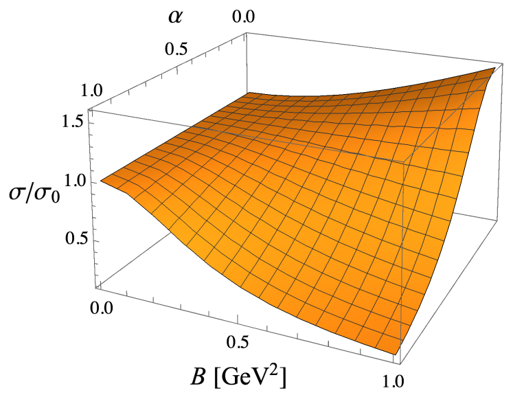
Figure 2: Longitudinal electric conductivity $\sigma_{\parallel}$ normalized by its value $\sigma_{0}$ at $\alpha=B=0$. The physical value of $\alpha$ is $3/4$, for which $\sigma_{\parallel}$ decreases with increasing $B$.

For $\alpha=0$ our numerical results in Fig. 1 correctly reproduce the increasing behavior as in Fig. 2. Also, there is no $\alpha$ dependence at all for $B=0$ since the Chern-Simons action has no contribution, which is confirmed in Fig. 2. It is intriguing to observe that the qualitative tendency of the $B$ dependence is changed as $\alpha$ increases. Indeed, for $\alpha=3/4$ (i.e., the physical value), $\sigma_{\parallel}(B)$ decreases with increasing $B$, and this is our central finding.

Actually, for $\alpha=0$, we can give a simple account for the increasing behavior of $\sigma_{\parallel}$. In the limit of strong $B$ the LLL approximation should be justified, and the fermion dynamics is reduced to (1+1) dimensions along the longitudinal direction. Then, massless fermions cannot scatter in (1+1) dimensions (see discussions in Ref. Fukushima et al. (2016)) and the transport coefficients are inevitably divergent Hattori and Satow (2016), see more specifically Fig. 3 in Ref. Fukushima and Hidaka (2018). This phase space argument has nothing to do with the chiral anomaly, so that it is applied to the $\alpha=0$ case. At the algebraic level we can understand $\sigma_{\parallel}\to\infty$ at strong $B$ from Eq. (40). For $\alpha=0$ and small $\Omega$, the differential equation to be solved corresponding to Eq. (21) is

$$\partial_{\xi}\Bigl{[}\xi(1-\xi^{3})\partial_{\xi}a_{z}\Bigr{]}=0$$ (44)

after we replace $\mathcal{B}\to B^{2}u_{T}^{-3}\xi^{3}$. The integration near $\xi\sim 0$ is singular, which makes $\sigma_{\parallel}$ divergent.

The situation is drastically changed by the third term $\propto\alpha^{2}$ in Eq. (40). In the large $B$ limit, again, the differential equation simplifies and the general solution can be expressed in terms of the hypergeometric functions. To meet the boundary condition near $\xi\sim 1$, the conductivity should come along with a normalization factor that is suppressed by $\alpha$. The third term in Eq. (40) was originally $4\alpha Ba_{0}^{\prime}$ and this is proportional to the matter chirality [i,e., the first term in Eq. (38)]. It is therefore the matter chirality that allows for fermion scatterings even at strong $B$. We have subtracted the zero mode (and divergent) contribution from the chiral anomaly, and yet, the nonzero mode (that is, $a_{z}-1$ is of order $\Omega$) still plays a role. This is a sensible scenario; the anomaly can generate the chirality, which in turn means that the chirality can decay via the anomaly. This is extremely interesting. We identified the Ohmic electric conductivity, but its properties reflect interactions induced by the chiral anomaly. A very favorable feature is that the anomaly dependence in the Ohmic part is opposite to the negative magnetoresistance expected in the zero mode.

V Summary

We calculated the magnetic field dependence of the electric conductivity in deconfined QCD matter using a holographic QCD model, namely, the Sakai-Sugimoto Model. For simplicity we considered only the high temperature environment at $T>T_{c}$ and solved the equations of motion in the presence of external magnetic field $B$.

We first checked how far the model can work quantitatively by estimating the electric conductivity $\sigma$ at $B=0$. Because of a mass scale, the Kaluza-Klein mass $M_{\rm KK}$, the $T$ dependence is found to be $\sigma\propto T^{2}/M_{\rm KK}$, but as long as $T\gtrsim T_{c}$, we have verified that our estimates agree well with the lattice-QCD values.

We then proceed to the finite $B$ case, and we found that the transverse conductivity, $\sigma_{\perp}$, is suppressed by larger $B$, which is understandable from the Landau quantization picture. In contrast, the longitudinal conductivity, $\sigma_{\parallel}$, is an increasing function of $B$ if we drop the Chern-Simons action with $\alpha=0$. This is also intuitively understandable from the phase space argument in the lowest Landau level approximation. Massless fermions cannot scatter in effectively reduced (1+1) dimensions, and transport coefficients generally diverge. However, our numerical results for $\alpha\neq 0$ show a turnover; that is, $\alpha_{\parallel}$ decreases with increasing $\alpha$ and $B$. We gave a plain explanation on this numerical observation. That is, the zero mode contribution from the chiral anomaly yields the negative magnetoresistance (and it is divergent for massless fermions unless a relaxation time is introduced), and the nonzero mode contribution from the chiral anomaly can significantly affect the fermion interactions and even the Ohmic part of the electric conductivity. Fortunately, however, the $B$ dependence that we discovered in the Ohmic part is opposite to the negative magnetoresistance, and it would not impede a common interpretation of the negative magnetoresistance as a signature for the chiral magnetic effect.

There are several interesting directions for future investigations. In the present work we did not include a finite density effect, but the introduction of the chemical potential is feasible enough. Another improvement is to generalize the formulation to lower temperatures in the confined phase. In this case one needs to solve the equation of motion for $x_{4}$, and the calculations become technically involved, but still possible.

For more quantitatively serious discussions, we should compare the zero mode and the nonzero mode contributions, and for this, an extension to massive fermions is needed. Instead of it, one might think of introducing a parameter corresponding to a relaxation time in the equations of motion by hand, but the relaxation time may have nontrivial dependence on $B$, and such a handwaving treatment would loose the predictive power. In fact, the holographic model we employed here was the top-down one and we believe that our results are robust in some particular limit of QCD. In the bottom-up approach, on the other hand, some $B$ dependence may be hidden in model parameters and assumed geometries, and the predictive power would be limited.

During completion of the manuscript, we have learned a very interesting result in Ref. Sogabe et al. (2021); they found a positive magnetoresistance from hydrodynamic fluctuations. The claim seems to be consistent with what we found in Fig. 2 at $\alpha=3/4$. It is an interesting question whether their mechanism is totally distinct or has some connection to ours.