Two-dimensional spin models with macroscopic degeneracy

Abstract

We consider a class of anisotropic spin-$\frac{1}{2}$ models with competing ferro- and antiferromagnetic interactions on two-dimensional Tasaki and kagome lattices consisting of corner sharing triangles. For certain values of the interactions the ground state is macroscopically degenerated in zero magnetic field. In this case the ground state manifold consists of isolated magnons as well as the bound magnon complexes. The ground state degeneracy is estimated using a special form of exact wave function which admits arrow configuration representation on two-dimensional lattice. The comparison of this estimate with the result for some special exactly solved models shows that the used approach determines the number of the ground states with exponential accuracy. It is shown that the main contribution to the ground state degeneracy and the residual entropy is given by the bound magnon complexes.

I Introduction

Quantum magnets on geometrically frustrated lattices have attracted much interest in last year Diep ; Lacroice ; ModernPhysics . An important class of these systems includes lattices with magnetic ions located on vertices of connected triangles. For special relation between different exchange interactions such systems have a dispersionless one-magnon band ModernPhysics . There is a wide class of the frustrated quantum antiferromagnets (AF) in which a flat band exists Derg ; Zhitomirsky ; Tsun ; Derg1 ; Zhit ; Schulen . It includes the kagome and pyrochlor antiferromagnets. An interesting one-dimensional example of the flat-band antiferromagnet is the saw-tooth chain. The one-magnon flat-band leads to an existence of exact localized many-magnon states. In the antiferromagnetic flat-band models these states form the ground state manifold in the saturation magnetic field and the degeneracy grows exponentially in the thermodynamic limit giving a finite residual entropy Derg ; Zhitomirsky .

Another class of the frustrated quantum models with exact localized multi-magnon states are the models with competing ferro- and antiferromagnetic interactions (F-AF models). The zero-temperature phase diagram of these models has different phases depending on the ratio of the ferromagnetic and antiferromagnetic interactions. At the critical value of this ratio corresponding to a phase boundary the model has massively degenerated ground state manifold. One example of the F-AF systems is the same saw-tooth chain at the critical value of the frustration parameter $\alpha=\frac{J_{2}}{\left|J_{1}\right|}=\frac{1}{2}$, where $J_{2}$ and $J_{1}$ are AF and F interactions of the basal-basal and basal-apical spins, correspondingly Dmitriev . It is worth noting that this model describes the magnetic molecule $Fe_{10}Gd_{10}$ frustration parameter of which is close to the critical value Gd ; DKRS . The ground state spin of this molecule $S=60$ is one of the largest spin of a molecule.

The main difference between AF and F-AF models is the additional bound magnon complexes which are exact ground states at the critical value of the frustration parameter together with the independent localized magnons. It leads to the macroscopical degeneracy of the ground state in zero-magnetic field and the residual entropy is larger than that for the AF models. The residual entropy in zero-magnetic field leads to an efficient magnetic cooling cooling ; Dmitriev which is important from the practical point of view.

The saw-tooth model and special type of kagome-like stripes kagomestripe in the critical point are solved exactly in contrast with two-dimensional F-AF models. At the same time the degeneracy of the AF models and the residual entropy in the saturation field can be found by mapping the system of isolated localized magnons onto the classical lattice gas of hard-core particles Derg . However, such mapping does not work for the F-AF models due to the existence of the bound magnon complexes.

In recent papers 3-colors ; 3-colors1 the $s=\frac{1}{2}$ XXZ model on the two-dimensional lattices consisting of triangles has been studied for a special value of the ratio of the Ising $J_{z}$ to the antiferromagnetic transverse interaction $J$ ($\frac{J_{z}}{J}=-\frac{1}{2}$) when the ground state has macroscopic degeneracy in zero-magnetic field. It was shown earlier in Refs.Dmitriev1 ; Johann that this model has both localized many-magnon states and bound magnon complexes and all of them belong to the ground state manifold. It was shown in 3-colors ; 3-colors1 that the ground state can be described by ‘quantum three-coloring wave functions’. This approach is based on a representation of the exact ground states in terms of the wave functions denoted as colors on sites of the lattice and each site can be painted in one of three colors, while the nearest sites can not be the same color. We note, however, that the ‘three colors representation’ is applicable to the models with equal interactions between all nearest spins only.

In the present paper we extent this approach to a class of the spatially anisotropic F-AF two-dimensional models with the macroscopically degenerated ground state. Our main task is the calculation of the total number of the ground states, $W$. The macroscopic degeneracy means that $W$ grows exponentially in the thermodynamic limit, i.e $W\sim\xi^{N}$ ($N$ is number of spins) and we focus on the evaluation of $\xi$ and the corresponding entropy per spin $\mathcal{S=}\ln\xi$. In other words, we will estimate the exponential factor of the total degeneracy.

The paper is organized as follows. In Section II we establish necessary conditions on the Hamiltonian parameters for which the F-AF models have a massive degenerate ground state and consider some special cases of these parameters. In Section III we represent the exact ground state wave function of the system as a product of exact wave functions of the connected triangles and we give the lattice gas representation of this function in terms of configurations of arrows on the bond between two spins. As an example we apply this approach to the F-AF saw-tooth chain in the critical points and compare obtained results with the exact ones. In Section VI we estimate the total number of the degenerate ground states for the two-dimensional F-AF Tasaki and kagome lattices and compare the obtained results with exact diagonalization of finite systems. The conclusions are summarized in Section V.

II Anisotropic F-AF models with macroscopical ground state degeneracy

In this Section we find the general form of the Hamiltonian of the $s=\frac{1}{2}$ F-AF model consisting of corner-sharing triangles for which the model becomes flat-band one with highly degenerate ground state. The Hamiltonian of such model can be written as a sum of local Hamiltonians acting on triangles:

$$H=\sum H_{i}$$ (1)

The most general form of such local Hamiltonian commuting with the total $S_{tot}^{z}$ is

$$H_{1} = -J_{1}\left(s_{1}^{x}s_{2}^{x}+s_{1}^{y}s_{2}^{y}+\Delta_{1}(s_{1}^{z}s_{2}^{z}-\frac{1}{4})\right)-J_{2}\left(s_{2}^{x}s_{3}^{x}+s_{2}^{y}s_{3}^{y}+\Delta_{2}(s_{2}^{z}s_{3}^{z}-\frac{1}{4})\right)$$ (2)

$$+J_{AF}\left(s_{1}^{x}s_{3}^{x}+s_{1}^{y}s_{3}^{y}+\Delta(s_{1}^{z}s_{3}^{z}-\frac{1}{4})\right)$$

where the first two terms describe two ferromagnetic interactions and the third one describes antiferromagnetic interaction of spins on the triangle (see Fig.1). The constants in (2) are chosen so that the energy of the ferromagnetic state on triangle with $S^{z}=\pm\frac{3}{2}$ is zero. Further we scale the energy by the normalization $J_{AF}=1$.

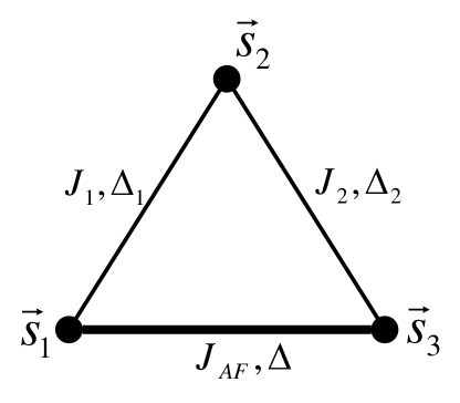
Figure 1: Local Hamiltonian on triangle.

When $J_{1}$ and $J_{2}$ are large the ground state of $H$ is ferromagnetic ($S_{tot}^{z}$ $=\frac{N}{2}$) with zero energy. At the transition points on the phase boundaries between the ferromagnetic and another phase (antiferromagnetic or ferrimagnetic ferri ) the ground state energy remains zero as well as the energy of $H_{1}$ with $S^{z}=\pm\frac{3}{2}$. As was shown in Ref.Dmitriev for the saw-tooth chain with equal ferromagnetic bonds ($J_{1}=J_{2}$, $\Delta_{1}=\Delta_{2}$) at the transition points the ground state is macroscopically degenerated and the spectrum of each local Hamiltonian (2) consists of two excited states with $S^{z}=\pm\frac{1}{2}$ and six ground states (two states with $S^{z}=\pm\frac{3}{2}$ and four states with $S^{z}=\pm\frac{1}{2}$). The same properties of local Hamiltonian remains for the saw-tooth chain with isotropic interactions ($\Delta_{i}=1$) but different ferromagnetic bonds $J_{1}\neq J_{2}$ kosoi . The local Hamiltonian which has the above spectrum can be written as a sum of two projectors on two excited states with arbitrary numerical factors. Therefore, we need to write down the general form of these excited states.

The basis for the system of three spins-$\frac{1}{2}$ in the sector with $S^{z}=\frac{1}{2}$ contains three states: $\left|\downarrow\uparrow\uparrow\right\rangle,\left|\uparrow\downarrow\uparrow\right\rangle,\left|\uparrow\uparrow\downarrow\right\rangle$ (and similar for the sector with $S^{z}=-\frac{1}{2}$). Therefore, any state with $S^{z}=\frac{1}{2}$ can be parameterized by two independent parameters. It is convenient to choose these parameters as two angles $\alpha$ and $\beta$, so that the excited states with $S^{z}=\pm\frac{1}{2}$ are written in the following form:

$$\chi_{-1/2} = \sin\beta\left|\uparrow\downarrow\downarrow\right\rangle-\sin(\alpha+\beta)\left|\downarrow\uparrow\downarrow\right\rangle+\sin\alpha\left|\downarrow\downarrow\uparrow\right\rangle$$ (3)

$$\chi_{1/2} = \sin\beta\left|\downarrow\uparrow\uparrow\right\rangle-\sin(\alpha+\beta)\left|\uparrow\downarrow\uparrow\right\rangle+\sin\alpha\left|\uparrow\uparrow\downarrow\right\rangle$$ (4)

Then, the ground state manifold contains two ferromagnetic states $\left|\downarrow\downarrow\downarrow\right\rangle$, $\left|\uparrow\uparrow\uparrow\right\rangle$ and four states with $S^{z}=\pm\frac{1}{2}$ orthogonal to the states $\chi_{\pm 1/2}$, which can be chosen as:

$$\phi_{-1/2} = \cos\alpha\left|\uparrow\downarrow\downarrow\right\rangle+\left|\downarrow\uparrow\downarrow\right\rangle+\cos\beta\left|\downarrow\downarrow\uparrow\right\rangle$$ (5)

$$\phi_{1/2} = \cos\alpha\left|\downarrow\uparrow\uparrow\right\rangle+\left|\uparrow\downarrow\uparrow\right\rangle+\cos\beta\left|\uparrow\uparrow\downarrow\right\rangle$$ (6)

$$\varphi_{-1/2} = \sin\alpha\left|\uparrow\downarrow\downarrow\right\rangle-\sin\beta\left|\downarrow\downarrow\uparrow\right\rangle$$ (7)

$$\varphi_{1/2} = \sin\alpha\left|\downarrow\uparrow\uparrow\right\rangle-\sin\beta\left|\uparrow\uparrow\downarrow\right\rangle$$ (8)

The interaction parameters of the local Hamiltonian (2) having the above spectrum is:

$$\Delta = \cos(\alpha+\beta)$$ (9)

$$J_{1} = \frac{\sin\left(\alpha+\beta\right)}{\sin\alpha}$$ (10)

$$J_{2} = \frac{\sin\left(\alpha+\beta\right)}{\sin\beta}$$ (11)

$$J_{1}\Delta_{1} = \cos(\alpha+\beta)+\frac{\sin\beta}{\sin\alpha}$$ (12)

$$J_{2}\Delta_{2} = \cos(\alpha+\beta)+\frac{\sin\alpha}{\sin\beta}$$ (13)

Energy of the excited states $\chi_{\pm 1/2}$ on triangle is

$$E=\cos(\alpha+\beta)+\frac{\sin\beta}{\sin\alpha}+\frac{\sin\alpha}{\sin\beta}$$ (14)

Both angles $\alpha$ and $\beta$ can be analytically continued. Since the parameters $J_{i}$ and $\Delta_{i}$ of the Hamiltonian (2) are real, $\alpha$ and $\beta$ can be either both real ($\Delta\leq 1$) or both imaginary ($\Delta>1$). For the case of imaginary $\alpha$ and $\beta$ we can use the same expressions for wave functions and Hamiltonian parameters just substituting $\alpha\to i\alpha$ and $\beta\to i\beta$ (so that, $\cos\to\cosh$ and $\sin\to\sinh$ everywhere):

$$\Delta = \cosh(\alpha+\beta)$$ (15)

$$J_{1} = \frac{\sinh\left(\alpha+\beta\right)}{\sinh\alpha}$$ (16)

$$J_{2} = \frac{\sinh\left(\alpha+\beta\right)}{\sinh\beta}$$ (17)

$$J_{1}\Delta_{1} = \cosh(\alpha+\beta)+\frac{\sinh\beta}{\sinh\alpha}$$ (18)

$$J_{2}\Delta_{2} = \cosh(\alpha+\beta)+\frac{\sinh\alpha}{\sinh\beta}$$ (19)

II.1 Special cases

Let us consider some special cases of the Hamiltonian $H$.

The case $\alpha=\beta$ corresponds to the Hamiltonian (2) with $\Delta=\cos(2\alpha)$ and equal ferromagnetic bonds ($\Delta_{1}=\Delta_{2}=\cos\alpha$ and $J_{1}=J_{2}=2\cos\alpha$). This case was studied in detail for saw-tooth chain in Ref.Dmitriev1 .

The case $\alpha\to 0$, $\beta\to 0$. This case describes the isotropic model ($\Delta=\Delta_{1}=\Delta_{2}=1$) with

$$J_{1} = 1+\frac{\beta}{\alpha}$$ (20)

$$J_{2} = 1+\frac{\alpha}{\beta}$$ (21)

so that $J_{1}$ and $J_{2}$ obey the relation: $J_{1}^{-1}+J_{2}^{-1}=1$. This case was studied for saw-tooth chain in detail in Ref.kosoi .

Special case $\alpha+\beta=\frac{\pi}{2}$. In this case $\Delta=0$ and the local Hamiltonian takes the form:

$$H_{1}=-\frac{1}{\sin\alpha}\left(s_{1}^{x}s_{2}^{x}+s_{1}^{y}s_{2}^{y}+\cos(\alpha)s_{1}^{z}s_{2}^{z}\right)-\frac{1}{\cos\alpha}\left(s_{2}^{x}s_{3}^{x}+s_{2}^{y}s_{3}^{y}+\sin(\alpha)s_{2}^{z}s_{3}^{z}\right)+\left(s_{1}^{x}s_{3}^{x}+s_{1}^{y}s_{3}^{y}\right)$$ (22)

Here for $\alpha=\beta=\frac{\pi}{4}$ we reproduce the special case $\Delta_{1}=\Delta_{2}=1/\sqrt{2}$ considered in our paper Dmitriev1 for the F-AF saw-tooth chain. This case is specific and it will be discussed below in detail. In this case the Hamiltonian (2) is

$$H_{S,1}=\left(s_{1}^{x}s_{3}^{x}+s_{1}^{y}s_{3}^{y}\right)-\sqrt{2}(s_{1}^{x}s_{2}^{x}+s_{1}^{y}s_{2}^{y})-s_{1}^{z}s_{2}^{z}-\sqrt{2}(s_{2}^{x}s_{3}^{x}+s_{2}^{y}s_{3}^{y})-s_{2}^{z}s_{3}^{z}$$ (23)

In case $\alpha\to 0$ and $\beta\to\frac{\pi}{2}$, the model has the isotropic ferromagnetic bond ($1-2$) slightly connected with the third spin by the $XY$ type interactions:

$$H_{1}=-\mathbf{\vec{s}}_{1}\cdot\mathbf{\vec{s}}_{2}-\alpha\left(s_{2}^{x}s_{3}^{x}+s_{2}^{y}s_{3}^{y}\right)+\alpha\left(s_{1}^{x}s_{3}^{x}+s_{1}^{y}s_{3}^{y}\right)$$ (24)

The case $\alpha=\beta=\frac{\pi}{3}$. In this case $J_{1}=$ $J_{2}=-1$, $\Delta_{1}=\Delta_{2}=\frac{1}{2}$, $\Delta=-\frac{1}{2}$. After rotation in the $XY$ plane $s_{n}^{x,y}\to(-1)^{n}s_{n}^{x,y}$ the local Hamiltonian takes the symmetric form

$$H_{1}=\left(s_{1}^{x}s_{2}^{x}+s_{1}^{y}s_{2}^{y}-\frac{1}{2}s_{1}^{z}s_{2}^{z}\right)+\left(s_{2}^{x}s_{3}^{x}+s_{2}^{y}s_{3}^{y}-\frac{1}{2}s_{2}^{z}s_{3}^{z}\right)+\left(s_{1}^{x}s_{3}^{x}+s_{1}^{y}s_{3}^{y}-\frac{1}{2}s_{1}^{z}s_{3}^{z}\right)$$ (25)

Exact ground state degeneracy for this model on saw-tooth chain was calculated in Ref.Dmitriev1 . Later this model was studied on kagome lattice in Ref.3-colors ; 3-colors1 using three-coloring representation of the ground state manifold.

The ‘imaginary’ case (15-19) with $\alpha\gg 1$ and $\beta\gg 1$. The Hamiltonian in this case becomes with the exponential accuracy (corrections of the order $\sim e^{-\alpha}$or $e^{-\beta}$):

$$H_{1}=\left(s_{1}^{z}s_{3}^{z}-s_{1}^{z}s_{2}^{z}-s_{2}^{z}s_{3}^{z}\right)-2e^{-\alpha}\left(s_{1}^{x}s_{2}^{x}+s_{1}^{y}s_{2}^{y}\right)-2e^{-\beta}\left(s_{2}^{x}s_{3}^{x}+s_{2}^{y}s_{3}^{y}\right)$$ (26)

The Ising part of the Hamiltonian $\left(s_{1}^{z}s_{3}^{z}-s_{1}^{z}s_{2}^{z}-s_{2}^{z}s_{3}^{z}\right)$ has the ground state degeneracy ($3^{n}+1$) on saw-tooth chain Dmitriev1 . The two last terms are $XY$ perturbations which partially split the degeneracy. The split excited states form multi-scale energy hierarchy Dmitriev1 .

The ‘imaginary’ case with $\alpha\ll 1$. In this case the model has the isotropic ferromagnetic bond ($1-2$) slightly connected with the third spin by $XXZ$ type with opposite signs of interactions between spins ($2,3$) and ($1,3$):

$$H_{1}=-\mathbf{\vec{s}}_{1}\cdot\mathbf{\vec{s}}_{2}-\frac{\alpha}{\sinh\beta}\left(s_{2}^{x}s_{3}^{x}+s_{2}^{y}s_{3}^{y}+\cosh(\beta)s_{2}^{z}s_{3}^{z}\right)+\frac{\alpha}{\sinh\beta}\left(s_{1}^{x}s_{3}^{x}+s_{1}^{y}s_{3}^{y}+\cosh(\beta)s_{1}^{z}s_{3}^{z}\right)$$ (27)

In the limit $\beta\gg 1$ only the Ising term survives in the 2-3 and 1-3 interactions and the model reduces to:

$$H_{1}=-\mathbf{\vec{s}}_{1}\cdot\mathbf{\vec{s}}_{2}-\alpha s_{2}^{z}s_{3}^{z}+\alpha s_{1}^{z}s_{3}^{z}$$ (28)

The latter model is similar to the model (24) but with the Ising type of small perturbations.

III Arrow configuration approach for the ground state with macroscopic degeneracy

The exact ground state degeneracy of the F-AF saw-tooth chain at the critical points has been found in Dmitriev ; Dmitriev1 . However, the consideration in Dmitriev ; Dmitriev1 was relied essentially on the one-dimensionality of the model and the methods used in Dmitriev ; Dmitriev1 are not applicable for the two-dimensional case. In this Section we will use another approach for the estimate of the ground state degeneracy and as an example we consider the F-AF saw-tooth chain.

First, we notice that four states $\phi_{\pm 1/2}$ and $\varphi_{\pm 1/2}$ (5-8) can be linearly transformed to four functions $\psi_{\pm 1/2}=\phi_{\pm 1/2}-i\varphi_{\pm 1/2}$ and $\psi_{\pm 1/2}^{\ast}=\phi_{\pm 1/2}+i\varphi_{\pm 1/2}$:

$$\psi_{-1/2} = \left(e^{-i\alpha}s_{1}^{+}+s_{2}^{+}+e^{i\beta}s_{3}^{+}\right)\left|\downarrow\downarrow\downarrow\right\rangle$$ (29)

$$\psi_{-1/2}^{\ast} = \left(e^{i\alpha}s_{1}^{+}+s_{2}^{+}+e^{-i\beta}s_{3}^{+}\right)\left|\downarrow\downarrow\downarrow\right\rangle$$ (30)

$$\psi_{1/2} = \left(e^{-i\alpha}s_{2}^{+}s_{3}^{+}+s_{1}^{+}s_{3}^{+}+e^{i\beta}s_{1}^{+}s_{2}^{+}\right)\left|\downarrow\downarrow\downarrow\right\rangle$$ (31)

$$\psi_{1/2}^{\ast} = \left(e^{i\alpha}s_{2}^{+}s_{3}^{+}+s_{1}^{+}s_{3}^{+}+e^{-i\beta}s_{1}^{+}s_{2}^{+}\right)\left|\downarrow\downarrow\downarrow\right\rangle$$ (32)

We look for the wave function of the ground state in the form:

$$\Psi=\prod(1+e^{i\varphi_{m}}s_{m}^{+})\left|\downarrow\downarrow\ldots\downarrow\right\rangle$$ (33)

where the product in Eq.(33) is taken over all sites. This wave function contains all possible values of $S_{tot}^{z}=-\frac{1}{2}N\ldots\frac{1}{2}N$ (it does not preserve total $S_{tot}^{z}$). The wave function (33) resembles three-coloring approach for the construction of the ground state 3-colors ; 3-colors1 .

Let us consider the the part of the wave function (33) corresponding to one isolated triangle. Its wave function

$$\Psi_{123}=(1+e^{i\varphi_{1}}s_{1}^{+})(1+e^{i\varphi_{2}}s_{2}^{+})(1+e^{i\varphi_{3}}s_{3}^{+})\left|\downarrow\downarrow\downarrow\right\rangle$$ (34)

is a superposition of both ferromagnetic states $\left|\downarrow\downarrow\downarrow\right\rangle$, $\left|\uparrow\uparrow\uparrow\right\rangle$ and the following wave functions with $S^{z}=\pm\frac{1}{2}$:

$$\psi_{-1/2} = \left(e^{i\varphi_{1}}s_{1}^{+}+e^{i\varphi_{2}}s_{2}^{+}+e^{i\varphi_{3}}s_{3}^{+}\right)\left|\downarrow\downarrow\downarrow\right\rangle$$ (35)

$$\psi_{1/2} = e^{i(\varphi_{1}+\varphi_{2}+\varphi_{3})}\left(e^{-i\varphi_{1}}s_{2}^{+}s_{3}^{+}+e^{-i\varphi_{2}}s_{1}^{+}s_{3}^{+}+e^{-i\varphi_{3}}s_{1}^{+}s_{2}^{+}\right)\left|\downarrow\downarrow\downarrow\right\rangle$$ (36)

Comparing the latter equations with expressions (29-32), we conclude that the condition to have $6$ ground states (5-8) and $2$ excited states (3,4) on the triangle requires that $\varphi_{2}=\varphi_{1}\pm\alpha$ and $\varphi_{3}=\varphi_{2}\pm\beta$. Thus, there are two possible angle configurations on triangle:

$$\{\varphi_{1},\varphi_{1}+\alpha,\varphi_{1}+\alpha+\beta\}$$

$$\{\varphi_{1},\varphi_{1}-\alpha,\varphi_{1}-\alpha-\beta\}$$ (37)

with arbitrary $\varphi_{1}$. These two conditions can be marked by arrows on AF bonds pointing in the direction of angle increase (see Fig.2). Then all allowed terms in wave function (33) can be represented graphically in a similar way. Therefore, there is an one-to-one correspondence between allowed terms in the function (33) and allowed configurations of the arrows. After this mapping the calculation of the number of the ground states is equivalent to counting of the allowed configurations of the arrows and this problem is reduced to the solution of the corresponding lattice gas model. We note that in this angle configuration approach (ACA) it is impossible to separate the contributions to the ground state degeneracy from the isolated localized magnons and from the bound magnon complexes. However, the number of isolated magnons can be found using the map to the hard-core representation Derg ; Zhitomirsky and comparison of it with the total number of allowed configurations gives the estimate of the contribution of complexes.

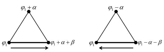
Figure 2: Two angle configurations on triangle indicated by a right and a left arrows.

As an example of an application of ACA approach, we calculate the ground state degeneracy of the saw-tooth chain at the critical point. There are two allowed configurations on each triangle and $2^{n}$ configurations ($n=\frac{N}{2}$ is number of triangles) on chain of triangles, and so, $2^{n}$ different wave functions (33). Each such function contains $N+1$ terms with different $S_{tot}^{z}$. Hence, we have $W=(2n+1)2^{n}$ ground state wave functions. It is interesting to compare this estimate with the exact results for $W$ obtained in Dmitriev ; Dmitriev1 . Exact value $W$ is proportional to $2^{n}$ though a pre-exponential factor $f(n)$ is different for different special cases. For example, $f(n)=(\frac{n}{2}+1)$ for $\alpha=\beta=\frac{\pi}{4}$ and $f(n)=(\frac{n}{3}+1)$ for $\alpha=\beta=\frac{\pi}{3}$. For the isotropic model $W=\sqrt{\frac{2n}{\pi}}2^{n}$. We see that the estimate of the ground state degeneracy based on the wave function (33) and counting of the allowed arrow configurations gives correct value for the exponent and thus, correctly reproduces the value of the residual entropy.

We have to make two remarks concerning the wave function (33). The first one is related to the mixing in Eq.(33) of states with different $S^{z}$ subspaces. Therefore, it is necessary to project wave function (33) to state with fixed $S^{z}$. The second remark concerns the problem of linear independence of the states corresponding to different arrow configurations in (33). These problems can be solved for finite systems, as was performed for the special case $\alpha=\beta=\frac{\pi}{3}$ in 3-colors ; 3-colors1 , but it is not clear how to solve them in the thermodynamic limit.

Nevertheless, the consideration of the F-AF saw-tooth chain shows that the total number of degenerate ground states coincides with exact $W$ up to preexponential factor. One can assume that the ACA approach provides this accuracy for the two-dimensional models considered in the next Section as well.

IV Ground state degeneracy for the Tasaki and kagome lattices

In this Section we consider the F-AF models with the macroscopic ground state degeneracy in the two-dimensional Tasaki lattice Tasaki . The Tasaki lattice is decorated square lattice consisting of corner sharing triangles as it is shown in Fig.3. The F-AF model on this lattice is a generalization of the F-AF saw-tooth chain to the two-dimensional case. The corresponding local Hamiltonian on each triangle has the form (2), where interaction between the basal spins forming square lattice is antiferrmagnetic and for simplicity we take equal ferromagnetic bonds: $J_{1}=J_{2}$ and $\Delta_{1}=\Delta_{2}$.

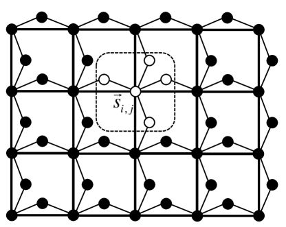
Figure 3: Tasaki lattice with outlined trapping cell occupied by the localized magnon on site ($i,j$).

We consider this model at the transition points between the ferromagnetic and other ground state phases (antiferromagnetic or ferrimagnetic) when the F and AF interactions satisfy conditions given in Section II. Then the model in zero-magnetic field has the ground state consisting of the independent localized magnons and the bound magnon complexes. The magnons are localized in trapping cells and each trapping cell consists of one site of an underlaying square lattice and four neighboring decorating sites, as shown in Fig.3. The wave function of one localized magnon on site ($i,j$) has a form

$$\hat{\varphi}_{i,j}\left|\downarrow\downarrow\ldots\downarrow\right\rangle=[2\Delta_{1}s_{i,j}^{+}+s_{i,j\pm\frac{1}{2}}^{+}+s_{i\pm\frac{1}{2},j}^{+}]\left|\downarrow\downarrow\ldots\downarrow\right\rangle$$ (38)

The bound magnon complexes contain overlapping localized magnons. For example, two-magnon complex with the center on site ($i,j$) is

$$\hat{\varphi}_{i,j}[(2\Delta_{1}^{2}-1)\hat{\varphi}_{i,j}+\hat{\varphi}_{i,j\pm 1}+\hat{\varphi}_{i\pm 1,j}]\left|\downarrow\downarrow\ldots\downarrow\right\rangle$$ (39)

The number of the independent localized magnons can be found by mapping to the hard-square model. The partition function of the latter is known Baxter and it is $Z=W_{0}\approx 1.5033^{N}$ ($N$ is number of squares in the lattice). However, it is not the case for the contribution of magnon complexes to the ground state manifold, because mapping them to any classical lattice model is unknown. Therefore, we use the ground state function (33) and its arrow representation for an estimate of $W$ .

Table 1: Maximal eigenvalue $\lambda_{L}$ of transfer-matrix for Tasaki stripe of width $L$ and the ratio $\lambda_{L}/\lambda_{L-1}$ in parenthesis.

L	Case $(\alpha+\beta)\neq\frac{\pi}{2}$	Case $(\alpha+\beta)=\frac{\pi}{2}$
1	2	2
2	3 (1.5)	4 (2)
3	4.562 (1.521)	8 (2)
4	6.972 (1.528)	16 (2)

As shown in Fig.2, the change of the angle along AF bonds is $\pm(\alpha+\beta)$. Requirement that the angle change along any closed loop on square lattice be zero leads to the selection rule on the allowed configurations of arrows on each elementary square: two arrows must be directed clockwise and two arrows are directed counter-clockwise. This condition allows only 6 arrow configuration out of 16 total on each elementary square, as shown in Fig.4. The number of allowed configurations on a Tasaki stripe of finite width $L$ and infinite length $n$ ($n\gg 1$) is given by the largest eigenvalue, $\lambda_{L}$, of the corresponding transfer-matrix, so that $W(L)=\lambda_{L}^{n}$. The results for $\lambda_{L}$ for $L=1,2,3,4$ are presented in Table 1 in the second column. For extrapolation of these results to $L\to\infty$ we follow the ratio $\lambda_{L}/\lambda_{L-1}$ and found that $\lambda_{L}/\lambda_{L-1}\to\xi\approx 1.54$. This means that the ground state degeneracy for large square lattice $L\times n$ behaves as $W=\xi^{N}$ where $N=nL$.

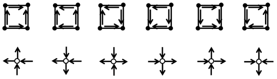
Figure 4: Six allowed arrow configurations on elementary square (top) of Tasaki lattice and six corresponding vertex configurations (bottom).

It is worth noting that the above problem of counting of all allowed arrow configurations on square lattice can be mapped to the six-vertex model (square-ice model). For this purpose one should consider each elementary square of Tasaki lattice as a new vertex and rotate all arrows on $90^{\circ}$ clockwise (or counterclockwise). As a result of this procedure $6$ allowed arrow configurations on elementary square are mapped to the $6$ types of vertex, as shown in Fig.4. The partition function of the six-vertex model was found by Lieb Lieb : $W=(4/3)^{3N/2}\approx 1.54^{N}$, which perfectly coincides with our extrapolation value. As we can see from a comparison of $W$ and $W_{0}$ the magnon complexes give main contribution to the ground state degeneracy in the thermodynamic limit, though for finite systems the contribution of the independent localized magnons can be essential. Taking into account that there are three spins per site in the square lattice the residual entropy per spin is $\mathcal{S}=\frac{1}{3}\ln\xi=0.144$.

Now we consider the special case $(\alpha+\beta)=\frac{\pi}{2}$ on Tasaki lattice. For this case the number of allowed configurations is larger than for other cases. This is due to the existence of two additional allowed arrow configurations in each elementary square: all four arrows are directed clockwise or counter-clockwise. These two extra configurations gives the change of angles around the square equal to $\pm 2\pi$ for $(\alpha+\beta)=\frac{\pi}{2}$. The largest eigenvalues of the transfer-matrix for stripe of finite width $L$ for this case are $\lambda_{L}=2^{L}$, as shown in Table 1, which means $\xi=2$. This result is in agreement with that for the eight-vertex model, where $W=2^{N}$ Baxter3 . The residual entropy per spin in this case is $\mathcal{S}=\frac{1}{3}\ln 2=0.231$.

Table 2: Ground state degeneracy of Tasaki stripe $2\times n$

n	Isotropic model	Case $(\alpha+\beta)=\frac{\pi}{2}$
2	52	64
3	158	128
4	632	1792
5	1882	2048
6	6884	40960

In order to verify the above ACA results we performed numerical calculations of quantum spin model (1). Unfortunately, the size of the system accessible for numerical calculations on Tasaki lattice is very limited, because Tasaki lattice contains three spins per site. Therefore, we had to restrict ourselves to exact diagonalization (ED) of Tasaki stripes $2\times n$ with $n\leq 6$. The results are presented in Table 2. As follows from Table 2, the ground state degeneracy for the special case $(\alpha+\beta)=\frac{\pi}{2}$ is higher than that for the isotropic case. The isotropic case can be considered as the general case, because all other cases of $\alpha$ and $\beta$ (except the case $(\alpha+\beta)=\frac{\pi}{2}$) have the same or very close ground state degeneracy. The extrapolation of the data for the isotropic case shows the exponent $\lambda_{2}\simeq 3\div 3.5$, which is in a good agreement with the estimate $\lambda_{2}=3$, presented in Table 1 for the general case. This agreement allows us to expect that the ACA result $W=(4/3)^{3N/2}$ for the general case gives a good approximation of the ground state degeneracy on Tasaki lattice.

The higher ground state degeneracy for the special case $(\alpha+\beta)=\frac{\pi}{2}$ can be explained by the following property of the model with the Hamiltonian $H_{S,1}$ (23). As follows from Eq.(39) the magnon states $\varphi_{i,j}$ for this model can be located on any sites of the lattice including nearest neighbors. That is the two magnon states $\varphi_{i,j}\varphi_{i+1,j}$ and $\varphi_{i,j}\varphi_{i,j+1}$ are exact ground states at $(\alpha+\beta)=\frac{\pi}{2}$. This allows to find the ground state degeneracy exactly. For two-dimensional Tasaki model comprised of $N$ squares the exact number of ground states $G(N,k)$ in the spin sector $S_{tot}^{z}=\frac{3N}{2}-k$ reduces to the number of possible combinations to place $k$ local magnon functions $\varphi_{i,j}$ in $N$ sites. It is given by the binomial coefficients $G(N,k)=C_{N}^{k}$ and, therefore, the total degeneracy is $W=2\cdot 2^{N}$ (the factor $2$ comes from two sectors $S^{z}_{tot}>0$ and $S^{z}_{tot}<0$ giving equal contribution). This is a correct result for any size of Tasaki lattice $L\times n$ except the case when both $n$ and $L$ are even numbers. In this case the exact number of ground states $G(N,k)$ is

$$G(N,k)=\sum_{m=0,2\ldots}^{k}C_{N}^{m}$$ (40)

for even $k$ and

$$G(N,k)=\sum_{m=1,3\ldots}^{k}C_{N}^{m}$$ (41)

for odd $k$. So that the total degeneracy is

$$W=\sum_{k}G(N,k)=2^{N}\left(N+1\right)$$ (42)

For Tasaki stripe $2\times n$ the total degeneracy has slightly different expression: $W=2^{2n-1}(3n+2)$. It is caused by the different number of spins per square: $3$ apical and $2$ basal spins for Tasaki stripe and $2$ apical and $1$ basal spin for Tasaki lattice.

In the thermodynamic limit all results for $W$ gives the same residual entropy per spin $\mathcal{S}=\frac{1}{3}\ln 2$. The above expressions are confirmed by ED results for $2\times n$ stripe presented in Table 2 and on Tasaki lattices $3\times 3$, $3\times 4$, $4\times 4$.

Another exact result for the model (23) is related to the spontaneous magnetization at $T=0$. The partition function $Z$ from the degenerate ground state in the magnetic field $h$ is

$$Z=2\sum_{k}G(N,k)\cosh[(\frac{3}{2}N-k)\frac{h}{T}]$$ (43)

The magnetization per spin $m$ is given by conventional thermodynamic equation:

$$m=\frac{T}{3N}\frac{\partial\ln Z}{\partial h}$$ (44)

The calculation of $Z$ results in the expression for the magnetization at $N\gg 1$ in a form

$$m=\frac{3+\exp(-h/T)}{6(1+\exp(-h/T))}$$ (45)

At $h/T\to 0$ the spontaneous magnetization is $m=\frac{1}{3}$. It means that the ground state is magnetically ordered and the magnetization is changed from $m=\frac{1}{2}$ in the ferromagnetic phase to $m=\frac{1}{3}$ on the phase boundary. Unfortunately, we can not calculate the magnetization for the cases $(\alpha+\beta)\neq\frac{\pi}{2}$ but we believe that the spontaneous magnetization exists for the general case of model (1).

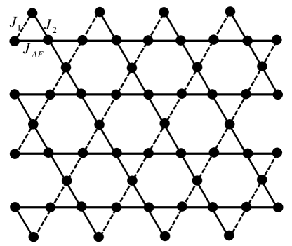
Figure 5: Kagome lattice with three different type of interactions.

Thus, the ACA approach correctly distinguishes the general case and the special case $(\alpha+\beta)=\frac{\pi}{2}$ on Tasaki lattice, gives a good approximation for the ground state degeneracy in the general case and reproduces the exact result for the special case. Unfortunately, the ACA approach does not work in general case for the F-AF model (1) on the kagome lattice shown in Fig.5. The point is that the total number of arrow configuration is strongly reduced by the self-consistency condition of zero angle change around each hexagon of kagome lattice, similar to the selection rule for elementary square on Tasaki lattice. The angle distribution of each hexagon is governed by the arrow configuration on six adjacent triangles. The total number of arrow configurations on six adjacent triangles is $2^{6}=64$. However, for general choice of $\alpha$ and $\beta$ only $10$ arrow configurations are allowed, one of which is shown in Fig.6.

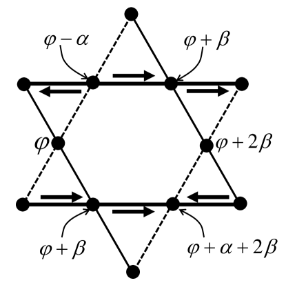
Figure 6: Example of possible arrow configuration around one hexagon and corresponding angles on hexagon sites.

The calculation of the number of the allowed arrow configurations on kagome lattice is very complicated problem. Therefore, at first we consider the kagome stripe of width $L=2$ shown in Fig.7. The maximal eigenvalue of the corresponding transfer-matrix is $\lambda_{2}=3$, so that the number of allowed arrow configurations on the kagome stripe is $W=3^{n}$, where $n$ is the number of elementary cells containing $7$ spins (see Fig.7). Similar calculations for the kagome stripe of width $L=3$ leads to $\lambda_{3}=2.618$ and we also note that the kagome stripe of width $L=1$ is nothing but the saw-tooth chain with $\lambda_{1}=4$ (three spins per elementary cell). Therefore, we see that $\lambda_{L}$ decreases with the increase of $L$ and tends to some value $\lambda_{\infty}$, which implies that for infinite kagome lattice ($L\to\infty$) the number of arrow configurations behaves as $W=\lambda_{\infty}^{n}$. Such dependence leads to zero residual entropy per spin $\mathcal{S}=\ln\lambda_{\infty}/L\to 0$.

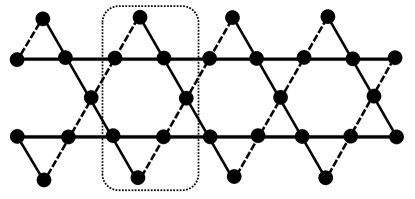
Figure 7: Kagome stripe with outlined elementary cell.

There are several special cases ($\alpha=\beta$, $\alpha+\beta=\frac{\pi}{2}$, $\alpha+2\beta=\pi$,$\ldots$), which have higher number of allowed arrow configurations per hexagon caused by commensurability of $\alpha$ and $\beta$ and/or the possibility for the angle change around the hexagon to be $\pm 2\pi$. However, the diagonalization of the corresponding transfer-matrix for kagome stripe of widths $L=1,2,3$ showed that the maximal eigenvalues $\lambda_{L}$ do not increase with the increase of $L$ and, therefore, there is no residual entropy. The only exception is the special case $\alpha=\beta=\frac{\pi}{3}$ with local Hamiltonian given by Eq.(25), which can be described by the three coloring approach 3-colors ; 3-colors1 . In this case the number of allowed arrow configurations per hexagon is $22$ and the calculated eigenvalues are $\lambda_{1}=4$, $\lambda_{2}=5.562$, $\lambda_{3}=7.894$. The ratios $\lambda_{2}/\lambda_{1}=1.39$ and $\lambda_{3}/\lambda_{2}=1.419$ converge to the exact result $\xi=1.461$ Baxter1 , so that the total number of arrow configurations is $W\approx 1.461^{N}$ for the kagome-lattice containing $N$ hexagons. This value should be compared with the number of the isolated magnons $W_{0}$, which is given by the hard hexagon model having $W_{0}\approx 1.395^{N}$ configurations Baxter2 . Therefore, we conclude that the main contribution to the ground state degeneracy in this case is given by the magnon complexes again.

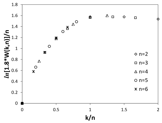
Figure 8: Dependence of number of ground states $W(k,n)$ on number of magnons $k$ for kagome stripe of width $L=2$ and length $n$ for the case $\alpha=\beta=\frac{\pi}{3}$.

We performed ED calculations for some special cases (including the isotropic version) of the quantum spin F-AF model (1) on the kagome-stripe of width $L=2$ and length $n\leq 6$ (Fig.7). The obtained data for the number of ground states $W(k,n)$ in different sectors of $S^{z}=S^{z}_{\max}-k$ for the case $\alpha=\beta=\frac{\pi}{3}$ are plotted in Fig.8 as $\ln(1.8W(k,n))/n$ vs. $k/n$. (Here the factor $1.8$ is fitting parameter, which describes $1/n$ corrections.) We see that the data for different $k$ and $n$ lies perfectly on one curve, which justifies the law $W(k,n)\sim\exp[nf(k/n)]$. The total number of ground states are defined by the maximum of this dependence, which takes place at $k\sim 1.2n$ and has the value $\simeq 1.6$. This allows to determine the thermodynamic behavior $W\sim\exp(1.6n)\simeq 5^{n}$, which is in a good agreement with the estimate of ACA approach for this case $\lambda_{2}=5.562$.

The same treatment of the numerical data for the case $\alpha=\beta=\frac{\pi}{4}$ and for the isotropic model leads to the results $W\simeq 5^{n}$ and $W\simeq 4.5^{n}$, respectively. Unfortunately, the ED calculations of the F-AF model for the kagome stripes with $L>2$ and rather large $n$ are not accessible. However, the fact that the number of ground states for kagome stripe with $L=2$ grows faster than $4^{n}$, which corresponds to $L=1$ (saw-tooth chain), is a strong argue in favor of the fact that the considered F-AF models on the kagome lattice have the macroscopic ground state degeneracy. Moreover, we can give the lower bound for $W$ demonstrating that $\xi>1$. Because $W>W_{0}$ the lower bound for $W$ is the number of the isolated magnons $W_{0}$. The value of $W_{0}$ can be found using the map of the considered models on the kagome lattice onto the lattice gas of hard-core particles. For the case $\alpha+\beta\neq\frac{\pi}{2}$ it is a hard-hexagon model (the triangular lattice with nearest-neighbor exclusion) and $W_{0}=1.395^{N}$ Baxter2 . For the case $\alpha=\beta=\frac{\pi}{4}$ it can be shown that the nearest-neighbor exclusion does not act between nearest-neighbor sites in the same stripe and the corresponding lattice-gas model reduces to the hard-square lattice. In this case $W_{0}=1.503^{N}$ Baxter2 . Therefore, for all considered models $\xi>1$.

V Summary

In this paper we study the ground state degeneracy of frustrated quantum spin-$\frac{1}{2}$ F-AF model at the critical ratio of the ferromagnetic and antiferromagnetic interactions corresponding to the boundaries of the ground state phase diagram. We constructed the general form of the anisotropic Hamiltonian acting on a lattice consisting of corner sharing triangles, the ground state of which is macroscopically degenerated in zero magnetic field. This general form of Hamiltonian is parameterized by two angles $\alpha$ and $\beta$.

To calculate the number of the degenerate ground states we use the wave function of the specific form (33). This function can be represented in terms of allowed arrow configurations on the corresponding lattice and the number of these configurations gives the estimate of the ground state degeneracy. This ACA approach reproduces the known exact result for the F-AF saw-tooth chain in the critical points with the exponential accuracy.

For two-dimensional Tasaki model the ACA approach correctly distinguishes the general case and the special case $(\alpha+\beta)=\frac{\pi}{2}$ giving different estimate of the ground state degeneracy, $W=1.5396^{N}$ for the general case and $W=2^{N}$ for the special case $(\alpha+\beta)=\frac{\pi}{2}$. Performed exact diagonalization calculations on finite parts of Tasaki lattice confirm macroscopic degeneracy of the ground state and show a good agreement with ACA results for the general case. For the special case $(\alpha+\beta)=\frac{\pi}{2}$ the ground state degeneracy is calculated exactly, it is $W\sim 2^{N}$ at $N\to\infty$ as correctly predicted by ACA approach.

The exact diagonalization of finite kagome lattices indicate the macroscopic ground state degeneracy for the general case on the kagome lattice. However, the ACA approach does not predict it. This is due to the fact that the number of allowed arrow configurations is strongly limited by the condition of zero total angle change around each hexagon of the kagome lattice. The only case where the ACA predicts macroscopic ground state degeneracy is the special case $\alpha=\beta=\frac{\pi}{3}$, where the above constraint is not so severe and the ACA reproduces the exact result $W=1.461^{N}$. Comparing the kagome and Tasaki lattices, we assume that the ACA approach can correctly predict ground state degeneracy for such lattices where each triangle has one spin that does not simultaneously belong to an adjacent triangle.

The ground state manifold for all above cases and lattices consists of isolated magnons and the bound magnon complexes, $W=W_{0}+W_{b}$. The number of the independent localized magnons can be found by the mapping to the hard-square model with $W_{0}\approx 1.503^{N}$ for Tasaki lattice and to the hard-hexagon model with $W_{0}\approx 1.395^{N}$ for kagome lattice. As follows from the comparison of $W$ and $W_{0}$, the magnon complexes give always main contribution to the ground state degeneracy in the thermodynamic limit, though for finite systems the contribution of the independent localized magnons can be essential.

The special case $\alpha=\beta=\frac{\pi}{4}$, for which the Hamiltonian takes a simple form (23), requires a separate comment. In this case the local magnon states can be located on any sites of the Tasaki lattice including nearest neighbors. This leads to higher ground state degeneracy and allows to calculate it exactly. It is obvious that this special model can be extended to three-dimensional Tasaki lattice with similar exact result for the ground state degeneracy.

In this paper we paid attention only to the ground state degeneracy. However, as was shown for the saw-tooth chain Dmitriev1 , the spectrum of the studied models can have interesting and unusual features: exponentially low excitations and multi-scale hierarchy. Exact diagonalization of finite Tasaki and kagome systems indicates the presence of such extremely low excitations. However, the accessible for ED systems are too small for the quantitative analysis of the spectrum. This interesting problem requires further study.

References

- (1) C. Lacroix, P. Mendels and F. Mila, eds., Introduction to frustrated magnetism. Materials, Experiments, Theory (springer-Verlag, Berlin, 2011).
- (2) H. T. Diep (ed) 2013 Frustrated Spin Systems (Singapore; World Scientific).
- (3) O. Derzhko, J. Richter, M. Maksymenko, Int. J. Mod. Phys B 29, 153007 (2015).
- (4) O. Derzhko, J. Richter, Phys. Rev. B 70, 104415 (2004).
- (5) M. E. Zhitomirsky, H. Tsunetsugu, Phys. Rev. B 70, 100403(R) (2004).
- (6) M. E. Zhitomirsky, H. Tsunetsugu, Progr. Theor. Phys. Suppl. 160, 361 (2005).
- (7) O. Derzhko, J. Richter, Eur. Phys. J. B 52, 23 (2006).
- (8) M. E. Zhitomirsky, H. Tsunetsugu, Phys. Rev. B 75, 224416 (2007).
- (9) J. Schnack, J. Schulenberg, J. Richter, Phys. Rev. B 98, 094423 (2018).
- (10) V. Ya. Krivnov, D. V. Dmitriev, S. Nishimoto, S. -L. Drexsler, J. Richter, Phys. Rev. B 90, 014441 (2014).
- (11) A. Baniodeh, N. Magnani, Y. Lan, G. Buth, C. E. Anson, J. Richter, M. Affronte, J. Schnack, A. K. Powell, Quantum Matter, 3, 10 (2018).
- (12) D. V. Dmitriev, V. Ya. Krivnov, J. Richter, J. Schnack, Phys. Rev. B 99, 094410 (2019); Phys. Rev. B 101, 054427 (2020).
- (13) M. E. Zhitomirsky and A. Honecker, J. Stat. Mech.: Theory and Experiment 2004, P07012 (2004).
- (14) D. V. Dmitriev and V. Ya. Krivnov, J. Phys.: Condens. Matter 29, 215801 (2017).
- (15) H. J. Changlani, D. Kochkov, K. Kumar, B. K. Clark, E. Fradkin, Phys. Rev. Lett. 120, 117202 (2018).
- (16) H. J. Changlani, S. Pujari, C. -M. Chungr, B. K. Clark, Phys. Rev. B 99, 104433 (2019).
- (17) D. V. Dmitriev, V. Ya. Krivnov, Phys. Rev. B 92, 184422 (2015).
- (18) O. Derzhko, J. Schnack, D. V. Dmitriev, V. Ya. Krivnov, J. Richter, Eur. Phys. J. B 93, 161 (2020).
- (19) D. V. Dmitriev and V. Ya. Krivnov, J. Phys.: Condens. Matter 28, 506002 (2016); V. Ya. Krivnov and D. V. Dmitriev, Russian J. Phys. Chem. B, 15, 89 (2021).
- (20) D. V. Dmitriev and V. Ya. Krivnov, J. Phys.: Condens. Matter 30, 385803 (2018).
- (21) H. Tasaki, Phys. Rev. Lett. 69, 1608 (1992).
- (22) R. J. Baxter, Ann. Combinatorics 3, 191 (1999).
- (23) E. H. Lieb, Phys. Rev., 162, 162 (1967).
- (24) R. J. Baxter, J. Math. Phys. (N.J.) 11, 784 (1970).
- (25) R. J. Baxter, S. K. Tsang, J. Phys A 13, 1023 (1980).
- (26) R. J. Baxter, Exactly Solved Models in Statistical Mechanics (Academic, London, 1982).