On the Evaluation of Sequential Machine Learning for Network Intrusion Detection

Abstract.

Recent advances in deep learning renewed the research interests in machine learning for Network Intrusion Detection Systems (NIDS). Specifically, attention has been given to sequential learning models, due to their ability to extract the temporal characteristics of Network traffic Flows (NetFlows), and use them for NIDS tasks. However, the applications of these sequential models often consist of transferring and adapting methodologies directly from other fields, without an in-depth investigation on how to leverage the specific circumstances of cybersecurity scenarios; moreover, there is a lack of comprehensive studies on sequential models that rely on NetFlow data, which presents significant advantages over traditional full packet captures. We tackle this problem in this paper. We propose a detailed methodology to extract temporal sequences of NetFlows that denote patterns of malicious activities. Then, we apply this methodology to compare the efficacy of sequential learning models against traditional static learning models. In particular, we perform a fair comparison of a ‘sequential’ Long Short-Term Memory (LSTM) against a ‘static’ Feedforward Neural Networks (FNN) in distinct environments represented by two well-known datasets for NIDS: the CICIDS2017 and the CTU13. Our results highlight that LSTM achieves comparable performance to FNN in the CICIDS2017 with over 99.5% F1-score; while obtaining superior performance in the CTU13, with 95.7% F1-score against 91.5%. This paper thus paves the way to future applications of sequential learning models for NIDS.

1. Introduction

Network Intrusion Detection Systems (NIDS) are of paramount importance for the protection of network infrastructures. Many detailed works (e.g., (Mishra et al., 2018; Liao et al., 2013; Buczak and Guven, 2016; Khraisat et al., 2019)) highlighted the significant advances of NIDS, which are subject of continuous improvements. Indeed, NIDS must face significant challenges such as the ever-changing network environments as well as skilled and motivated adversaries. In particular, the recent promising successes in machine and deep learning renewed the interest in devising autonomous defensive systems (Buczak and Guven, 2016; Khraisat et al., 2019), giving life to a next generation of NIDS.

Among the plethora of proposals that exploit Machine Learning (ML) techniques, one promising direction seeks to leverage sequential learning methods that rely on the enticing idea that specific network events exhibit temporal patterns. When properly applied, sequential ML methods—and especially their “deep” variants—offer the appreciable opportunity to automatically extract these temporal patterns. These patterns can then be used to create conventional anomaly- or signature-based detection systems. Despite abundant literature, an effective and realistic deployment of sequential learning models for NIDS is yet a distant goal. For instance, identifying temporal patterns is challenging because many factors must be considered, such as, the adopted network protocols; the web-services employed by the network; and the possible threats that may target the network.

Moreover, the massive size and variability of modern network traffic data makes timely analyses based on traditional packet captures (PCAP) a difficult objective – which is further aggravated by the increasing usage of encrypted traffic. To mitigate this issue, many proposals (e.g., (Sperotto et al., 2010)) favor the inspection of Network Flows (NetFlows) instead of PCAP data. In this context, we make an intriguing observation: although it has been empirically shown that cyber-attacks exhibit temporal patterns that can be easily extracted at the packet level, it is less clear whether this is still true at the ‘higher’ NetFlow level. Indeed, temporal patterns within packets are not guaranteed to exist also in the corresponding NetFlows, which are metadata that summarize the corresponding PCAP data.

In this paper we devise a novel methodology for (i) investigating the existence of temporal patterns in malicious NetFlows; and, if such patterns exist, (ii) assess their effectiveness for detection purposes. The primary focus of past literature on sequential ML-NIDS is the proposal of solutions that “outperform” the state-of-the-art according to some performance metrics; however, the investigation of the actual benefits brought by these solutions is often neglected. In contrast, our objective is a preliminary analysis focused on the investigation of the existence, advantages and shortcoming brought by using temporal patterns at the NetFlow level for NIDS. To the best of our knowledge, this paper is the first effort that analyzes and performs a fair comparison of sequential ML models against their ‘static’ counterparts.

We experimentally evaluate the proposed methodology on two well-known and recent datasets for NIDS, the CTU13 (Garcia et al., 2014) and the CICIDS2017 (Sharafaldin et al., 2018). We apply our method to extract temporal patterns, and use such patterns to train and compare two Deep Learning (DL) algorithms: one based on Long-Short-Term-Memory (LSTM), which leverages sequential learning; and one based on Feedforward Neural Networks (FNN), which is a traditional ‘static’ learning method. Our results highlight that the patterns extracted by our method yield proficient detectors in the CICIDS2017 scenario, with both LSTM and FNN achieving over 99.5% F1-score; whereas the LSTM significantly outperforms the FNN detector in the CTU13 scenario, with 95.7% F1-score against 91.5%.

We are confident that this paper will shed some light on the application of sequential learning models for NetFlow-based NIDS. Our work thus paves the way to more reliable defensive platforms, which can jointly combine existing detection techniques with novel solutions that also consider the temporal axis.

To summarize the main contributions of this work:

• we devise an original method to extract temporal patterns from NetFlows that can be leveraged by sequential ML;

• we evaluate the proposed method to explore its benefits by performing a fair comparison of a ‘static’ FNN against a ‘sequential’ LSTM on two well-known datasets for NIDS.

The remainder of this paper is structured as follows. Section 2 discusses related work. Section 3 describes the proposed methodology for extracting temporal patterns in malicious NetFlows. Section 4 presents the experimental settings. Section 5 evaluates our proposed method. Section 6 concludes the paper with final remarks and future work.

2. Related Work

There exist many proposals for detecting malicious traffic by means of machine learning techniques (e.g., (Buczak and Guven, 2016; Mishra et al., 2018)). There is also abundant literature on time-based analyses for NIDS (e.g., (Apruzzese et al., 2017; Zhou and Lang, 2003)).

This paper lies at the intersection of these two application fields. Our objective is investigating the effectiveness of temporal relationships for ML-based NIDS (ML-NIDS), hence our literature review focuses on those proposals that leverage machine- and, specifically, deep-learning by considering also the temporal axis, usually through Recurrent Neural Networks (RNN).

Among the earliest successful applications of sequential learning models to NIDS there is the 2017 proposal in (Yin et al., 2017). Since then, several works have proposed learning models that extract temporal relationships in the network traffic and use them for ML purposes. We categorize and discuss such works on the basis of the approach used to extract the temporal patterns, namely: automatic approaches, where the temporal patterns are extracted through a pipeline that inspects the input data and automatically learns the most significant temporal features; manual approaches, where the temporal patterns are extracted exclusively on the basis of the input features.

We provide an overview of the major differences among related work in Table 1. This table shows the datasets considered, the employed DL techniques (CNN stands for Convolutional Neural Networks), and whether the approach is tailored for anomaly- or misuse-based NIDS.

Table 1. Overview of related work on sequential ML-NIDS.

	Paper	Datasets	Detection method	CNN	RNN	FNN
Automatic	(Han et al., 2020)	ISCX2012, CICIDS2017	misuse	✓	✓	$\times$
	(Pektaş and Acarman, 2019)	CTU13, ISOT	misuse	✓	✓	✓
	(Zhang et al., 2019)	CICIDS2017, CTU13	anomaly	✓	✓	$\times$
	(Sinha et al., 2019)	CTU13	misuse	$\times$	✓	$\times$
	(Wu and Guo, 2019)	NSLKDD, UNSW-NB15	misuse	✓	✓	$\times$
Manual	(Radford et al., 2018b)	CICIDS2017	anomaly	$\times$	✓	✓
	(Radford et al., 2018a)	ISCX2012	anomaly	$\times$	✓	✓
	(Gwon et al., 2019)	UNSW-NB15	misuse	$\times$	✓	$\times$
	(Kim et al., 2020)	CTU13	anomaly	$\times$	✓	$\times$
	(Torres et al., 2016)	CTU13	misuse	$\times$	✓	$\times$

We do not consider works whose proposal is evaluated exclusively on the (outdated and widely deprecated (Sharafaldin et al., 2018)) NSLKDD dataset (e.g. (Boukhalfa et al., 2020)), and that have been published recently (since 2017). Finally, although many works use RNN for NIDS (e.g., (Khan et al., 2019)), they often neglect considering temporal dependencies, hence we do not consider such works in our analysis.

2.1. Automatic extraction of features

These works rely on an end-to-end pipeline that leverages spatio-temporal dependencies, usually by means of CNN and RNN. The CNN automatically learns both spatial and temporal features, thus removing the need of manually extracting the features used to devise the detector. In some of these proposals (i.e., (Wu and Guo, 2019; Zhang et al., 2019)), the network traffic is inspected at the packet level by transforming each packet into an image. These images are first spatially analyzed through a CNN, and then, the feature maps describing packets are used to extract temporal patterns by means of sequential models.

The authors of (Han et al., 2020) proposed a Spatial and Temporal Aware Intrusion Detection Model (STIDM) composed of LeNet-5 and a modified version of the LSTM. LeNet-5 was used to extract spatial features, while the modified LSTM was used to extract temporal patterns by taking into account the time intervals between packet exchanges. STIDM was trained on truncated flows of multiple packets created by grouping on the tuple (SourceIP, SourcePort, DestinationIP, DestinationPort, Protocol). We observe that it is difficult to attribute the outstanding performance of STIDM to the CNN and/or the LSTM from the results shown in (Han et al., 2020). Furthermore, STIDM works on truncated sequences of packets, which makes determining the existence of temporal patterns in NetFlows unfeasible.

The approach in (Zhang et al., 2019) is similar to (Han et al., 2020), as they use the same STIDM structure to extract spatial features and temporal patterns, but the LSTM architecture is different. In this work, the overall model was used to analyze sequences of packets composed of only the first 160 bytes of every packet; then, the packets are aggregated by following the same five-tuple of STIDM, but only the first 10 packets in each sequence are considered. Similarly to (Han et al., 2020), from (Zhang et al., 2019) it is difficult to conclude anything about the existence temporal patterns among NetFlows and about the true benefits brought by the LSTM, since the results of the tested models (CNN, LSTM and CNN+LSTM) showed comparable performance.

A different proposal for a end-to-end pipeline is in (Wu and Guo, 2019). Here, instead of chaining a CNN with a LSTM (as in (Han et al., 2020)), the authors first create a block composed by these two techniques, and then stack many of these blocks obtaining higher abstraction levels. Although the final performance of such architecture achieves excellent results, the method for processing the input data is poorly described, and no information is provided as to how the temporal domain is used.

In (Sinha et al., 2019), the authors used a sequence of graphs to model the time evolution of the network traffic, in which nodes are the hosts (in the form of IP addresses) of the network, and edges are the packets exchanged by hosts. After generating these graphs, time series are extracted from each node by computing a set of graph-based features (e.g., in/out-degree, or in/out-neighbors). Then, such time series are divided in five overlapped time intervals, which are used to train a LSTM to detect malicious (i.e., anomalous) hosts. We observe that the approach in (Sinha et al., 2019) presents a heavy burden in terms of computational resources for its feature extraction; furthermore, dividing a time series into fixed intervals does not allow to infer long-lasting temporal patterns–despite obtaining encouraging detection results on the considered testbed. Finally, this approach focuses on analyzing PCAP data, and not on NetFlows.

The authors of (Pektaş and Acarman, 2019) propose an approach similar to (Sinha et al., 2019), but assume NetFlows as input. A single graph was extracted from the dataset, where nodes represent hosts (as IP addresses), while edges represent the NetFlows exchanged by the hosts; then, a statistical summary of the NetFlows between each pair of nodes is created. Such statistical summary is integrated with temporal features extracted from the sequence of connection states between each pair of nodes. Then, both the statistical summary and the temporal features are used to make the final inference throughout a FNN. What makes (Pektaş and Acarman, 2019) intriguing is that there is an actual benefit from using temporal features extracted from the connection states of NetFlows. However, it also demonstrated that using only the temporal features extracted from the connection states was not enough to achieve good detection.

To summarize, the major drawbacks of these approaches is their specificity to packet level analyses. Inferring spatial features from NetFlow data may still give a benefit, but the overall detection process must take into account the complex NetFlow semantic. Finally, none of these works prove the existence of malicious temporal patterns in NetFlows that are usable for ML-NIDS.

2.2. Manual extraction

These approaches use the features as they are provided in the input data; some preprocessing may occur, but there is no automatic feature extraction mechanism, that is, the features are not produced by any ML method.

In (Radford et al., 2018a), the authors use a bidirectional LSTM model to predict whether a communication was atypical or not. Specifically, they leverage Natural Language Processing by transforming NetFlows into ‘tokens’, where a token is defined as either a network port or a byte-port tuple. Then, these tokens were grouped by IP-pairs within hourly bins to form time-ordered sequences. This allowed the LSTM to learn a model of the benign traffic, which is used to detect anomalous communications. We observe, however, that the NetFlow semantic was used only to extract information on the byte-port tuple, which is a limitation in large networks with high diversity in the traffic. Moreover, having sequences focused on IP-pair and of limited duration does not imply that the learned temporal patterns (if any) are truly effective for NIDS.

In (Radford et al., 2018b), the authors extend (Radford et al., 2018a) by evaluating five different methods for aggregating NetFlow tokens in time-ordered sequences. They showed that different aggregation methods do not play an important role in training sequential models, due to negligible performance differences. While this observation might be true in their specific context, it is not applicable for our case. Indeed, we want our ML-NIDS to learn the temporal pattern of attacks, thus splitting the corresponding attack NetFlows is not viable: by doing so, we would break the temporal patterns (if they exist).

In (Kim et al., 2020), the authors propose a Recurrent Variational Autoencoder to detect botnet connections through anomaly detection. Their model is trained on certain botnet types and tested on unseen ones, showing good detection performance and demonstrating generalization capabilities. We point out that the generalization capabilities of some ML methods (and, specifically, of RNN) are an appreciable characteristic. However, the sequences used in (Kim et al., 2020) are created by aggregating NetFlows on their source IP, and then each sequence is reduced by summarizing NetFlows, therefore inducing loss of data which may break any temporal pattern.

In (Torres et al., 2016) a behavioral LSTM is devised to counter botnet attacks by analyzing the long-term traffic characteristics. Here, NetFlows are first aggregated into sequences according to a 4-tuple (source IP, destination IP, destination part, protocol); then, each NetFlow is vectorized with the behavioural model on the basis of three features: size, duration, periodicity. Although this work evaluates the prominent issues in training LSTM (e.g., data imbalance), it manually cherry picked the best features for detection. We do not make such assumption in this paper.

The LSTM is used also in (Gwon et al., 2019) to detect and classify malicious network packets. The authors evaluate the semantic of categorical features through embedding layers. Their results show that such layers do not improve the detection, and that the binary classification of LSTM achieves optimal performance ($99.75\%$ F1-score). However, the LSTM is trained on sequences of fixed length, and no information on how to determine such length is provided. As in (Torres et al., 2016), this paper cherry-picks the optimal thresholds that ensure best results on their specific testbed, with low practical value.

To summarize, these works have little realistic usage, and do not allow to assess the effectiveness of the extracted temporal patterns.

3. Proposed Solution

Our goal is to investigate the existence of temporal patterns in malicious NetFlows, and then explore the benefits of using these patterns in detecting malicious activities via machine learning. Hence, our first objective is the extraction of such temporal patterns. To this purpose, we propose an original method based on expert knowledge and network data analytics. Then, we need to verify if the extracted patterns are useful for detection purposes.

As explained in Section 2, many state-of-the-art approaches for extraction of temporal patterns have significant limitations. Thus, we propose an original method that aims at mitigating such deficiencies. The intention is to give more guarantees that the underlying temporal characteristics of different attacks are truly captured by the generated sequences, and are hence usable for efficient detection. In the remainder of this work, we will use the term ‘scenario’ to denote a complete ‘attack scenario’, i.e., a sequence of NetFlows that describes a specific attack scenario.

We first describe the threat model, the characteristics of the network environment and the assumptions required by our method (Section 3.1). Then we present our proposed method for creating scenarios (Section 3.2 and outline the characteristics of the sequential ML model (Section 3.3).

3.1. Threat Model and Assumptions

This paper makes the following assumptions about the attacker’s side, the considered network environment, and the input data required for creating the attack scenarios.

Attacker. We assume an attacker with the goal of either stealing sensitive data from, or disrupting the services provided or used by, the targeted organization. As is common in NIDS scenarios, the attacker is assumed to have established a foothold within the targeted network by compromising one (or more) of its most vulnerable hosts. The attacker does not have any information about the defensive mechanisms monitoring the organization; for example, the attacker does not know the datasets used to train ML-based NIDS. The attacker can interact with the network services accessible from within the organization network, but they do not have direct access to the NetFlow-exporter nor to any defensive system.

Environment. We assume the typical network environment spanning from dozens to hundreds of hosts that perform multiple network activities. The traffic generated by these hosts is first captured as PCAP data, and then transformed into NetFlows by means of any NetFlow-generation software. These extracted NetFlows are then analyzed by the NIDS, possibly after some preprocessing operations. We assume that the traffic generated by the most critical servers of the organization (to which the attacker has no access) is analyzed by dedicated mechanism.

Input Data. Our method requires a collection of NetFlows that are labelled according to the malicious network activities that they represent (or as ‘benign’ if they are not related to illegitimate actions). For each NetFlow, our method requires the following pieces of information: the timestamp, the Source/Destination ports, the protocol, the duration, the direction of the connection with respects to the network environment (i.e., inbound, outbound, or bidirectional), and optionally the specific attack type denoted by the label. Any additional piece of information is not required, but – if available – it can be freely added to the list of considered features to provide more fine-grained results.

In summary, our proposed method makes the assumptions typical of NIDS scenarios, and only requires the essential pieces of information obtainable from any NetFlow-generation software. The availability of labelled data is also a standard assumption in machine learning tasks.

3.2. Extraction of Attack Scenarios

Our method uses expert knowledge that can be applied to existing labelled NetFlow data to extract the attack scenarios.

The fundamental idea is to use the available information on a given set of NetFlow data to extract these scenarios. Such information can be readily acquired from the labels or the documentation of a dataset; or after exploratory data-analytics procedures. Our intuition is that if a specific attack presents temporal patterns, then such patterns should not depend on the benign traffic. Hence, we propose to isolate the specific attack types and, for each type, focus on the time-interval containing the malicious samples.

However, many obstacles must be overcome to increase the likelihood that the extracted scenarios are effective for detection.

A well-known issue in the application of ML-based approaches for NIDS is the strong unbalancing between the normal ‘benign’ traffic, and the malicious traffic. Indeed, contrarily to other domains where ML is applied, in cybersecurity the illegitimate samples represent rare events (e.g., (Apruzzese et al., 2017; Chuang and Wu, 2019)) which are several orders of magnitude inferior to the normal events occurring in a network. A strong data imbalance affects all types of ML applications; however, our time-sensitive context further aggravates this problem, because finding temporal patterns in the minority class is more difficult.

Therefore, in designing our proposed methodology for extracting the attack scenarios, we must first mitigate the unbalancing in the data. By doing so, we can improve the quality (in terms of detection efficacy) of the extracted temporal patterns. To mitigate the unbalancing problem, we leverage two observations:

1. the majority of the benign traffic that skews the distribution of a dataset presents similar characteristics, i.e., same protocols or same (service) ports, and can be partially discarded to increase the ‘weight’ of the malicious patterns;

2. some attacks exhibit periodic behaviours (also referred to as beaconing (Apruzzese et al., 2017)), and are executed in time intervals that, if found, can be used to “split” the scenario.

By combining these two observations, we propose to identify one or more separate scenarios for each attack type; such scenarios contain only those samples (benign and malicious) generated at the precise time intervals. Hence, we focus on pinpointing one or more time intervals for each attack, and then create a dedicated scenario for each time interval by including only those NetFlow samples occurring within the corresponding intervals. The remaining traffic samples are then discarded.

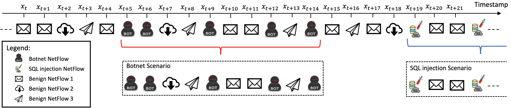
Figure 1. Example of attack scenarios creation. Any NetFlow not included in the attack scenarios is discarded.

Let us illustrate our idea with a concrete example, graphically depicted in Figure 1. Here, we assume that there exists a “Botnet Scenario” that starts from time $t+5$ (denoted with the NetFlow $x_{t+5}$), and ends at time $t+14$ (denoted with the NetFlow $x_{t+14}$). Our approach retains all NetFlows occurring within such time interval (spanning over 10 time-steps), regardless of their nature (benign or malicious). Specifically, the extracted “Botnet Scenario” will include two botnet NetFlows ($x_{t+5}$, $x_{t+6}$) followed by two benign NetFlows ($x_{t+7}$, $x_{t+8}$), and then by, in order, another botnet NetFlow ($x_{t+9}$), two benign NetFlows ($x_{t+10}$, $x_{t+11}$), a botnet NetFlow ($x_{t+12}$), a benign NetFlow ($x_{t+13}$), and the final botnet NetFlow ($x_{t+14}$) The NetFlows not included in such scenario (e.g., those from $x_{t}$ to $x_{t+4}$ and from $x_{t+15}$ to $x_{t+18}$) are discarded. Then, at time $t+19$, the “SQL Injection Scenario” begins.

The time intervals of an attack can be identified by analyzing the temporal distribution of malicious NetFlows (e.g., through the use of autocorrelation (Shirani et al., 2015)). However, such intervals can be obtained also from a dataset documentation (e.g., (Sharafaldin et al., 2018)).

When identifying the time-intervals of the attack scenarios, it is important to avoid ‘removing’ excessive amounts of benign samples: such occurrences may lead to oversimplified attack scenarios that are not sufficiently representative for detection purposes. If the extracted scenarios do not include at least some benign samples, we recommend increasing the length of the time-intervals to include more benign activities; alternatively, it is even possible to create dedicated ‘benign’ scenarios. We anticipate that, in our evaluation, we demonstrate that this latter technique can be used without affecting the learning phase of the sequential models.

Nonetheless, there may also exist some circumstances that lead to scenarios with an overabundance of benign samples (e.g., long duration attacks such as DDoS). Completely solving this issue is unfeasible. Hence, to mitigate this problem, we recommend to configure the loss function (i.e., the weights) of the ML model to assign a heavier penalty to misclassifications of malicious scenarios.

Let us explain the motivation behind such design choices. The ML literature proposes many techniques for dealing with imbalanced datasets. Some prominent examples involve: under-sampling the majority class or over-sampling the minority class (Cieslak et al., 2006); Synthetic Minority Over-sampling Technique (SMOTE) (e.g., (Zhang et al., 2020)); and weighing the loss function. However, with the exception of weighing of the loss function (which is the approach adopted in the proposed method), all these techniques artificially modify the input data and cannot be readily applied. Indeed, manipulating the network data with under/over-sampling may lead to biased and overfit models that learn unrealistic patterns, which may present good results on the ‘modified’ source dataset, but with impractical performance in realistic applications. We argue that these techniques are effective for training successful ML models that do not take into account temporal relationships. However, in our time-sensitive context, we have to ensure that the generation of synthetic data - or the removal of real data - does not interfere with the actual temporal patterns that denote the network activities.

Our method is among the first attempts in this domain, and presents much room for improvement. The major advantage of the proposed method, that is, creating specific attack scenarios, is that it should improve the quality of the learning phase by reducing the noise caused by the benign traffic. However, we stress that there is no guarantee that the extracted scenarios capture meaningful temporal relationships that are truly useful for detection purposes. This is why we must resort on ML methods to validate if the proposed method is effective or not.

3.3. Sequential ML for NIDS

To assess the quality of the temporal patterns hopefully contained in the attack scenarios (described in Section 3.2), we employ the de-facto sequence model for practical applications, gated RNN (Dey and Salem, 2017). Among the possible architectures of gated RNNs, we chose the Long Short-Term Memory (LSTM), due to its successful results achieved in literature (e.g., (Yeom et al., 2021; Mirza and Cosan, 2018)).

The successful principle at the base of the LSTM is an internal and context-aware self-loop, which dynamically adjusts its time scale on the basis of the sequence provided as input (Sainath et al., 2015). The ability of automatically adjusting the time scale makes LSTM a suitable candidate for our objective. Indeed, we stress that our method does not know whether temporal patterns (among malicious NetFlow data) exist or not. Moreover, even if such patterns exist, the method does not know when they occur and how long they last. Hence, we require a technique that is able to learn both long-term and short-term dependencies in the input scenarios. As an additional benefit, LSTM are among the best models for dealing with the so called vanishing gradient problem (Fei and Tan, 2018), which is a major obstacle when training RNN methods.

We propose the use of an unidirectional $n$-stacked version of the LSTM. We provide a schematic depiction of such architecture (in a 2-stacked version) in Figure 2, which reports the exemplary case of the Botnet attack scenario shown in Figure 1. As described in (Pascanu et al., 2013), having a stacked version of a RNN helps the model to look at the input data from different time-scales. This is possible since the input of each layer is the hidden state of the previous layer, with the sole exception of the very first layer which receives the actual input $x_{t}$.

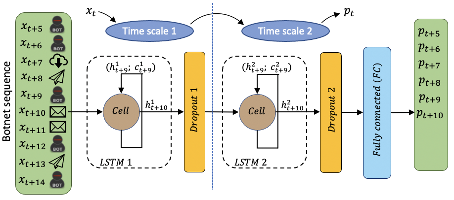
Figure 2. Exemplary architecture of a 2-stacked LSTM.

As shown in Figure 2, in a $n$-stacked version of a LSTM, the input at time-step $t$ is fed into the first layer, and it is then used (alongside the hidden state of the previous time-step $h_{t-1}^{1}$) to produce the Cell state $c_{t}^{1}$ (we use the superscript for identifying each layer). Then, for all the upper $n-1$ layers, the input at time-step $t$ is the hidden state of the previous layer, that is, for a layer $i\geq 2$, the input at time-step $t$ is $h_{t}^{i-1}$. This mechanism allows to bring the actual input into different time scales before making the final inference.

A common problem in any ML approach is the risk of realizing an overfit model. Depending on the input data and the chosen ML algorithm, different techniques can be used to remove (or mitigate) such issues (e.g., (Jindal et al., 2016)). Similarly, the activation function of the LSTM layers can be chosen arbitrarily: common solutions are, e.g., the sigmoid or the rectified linear unit (ReLU).

The model is used in a many-to-many fashion, that is, each NetFlow in a scenario is classified as either benign or malicious. This final classification is achieved through a single fully-connected neuronal layer placed after the last LSTM layer.

4. Experimental Settings

We experimentally evaluate the proposed methodology. Recall the twofold goal of our paper: investigating the existence of malicious temporal patterns in NetFlows; and verifying whether sequential learning models really learn and benefit from these patterns. To this purpose, we need to first devise a sequential learning model using some input data, and then compare its performance against a baseline ‘static’ ML model (using the same input data), but that does not consider any temporal relationship.

We describe the experimental settings to highlight the realistic value of our testbed. We present the chosen datasets in Section 4.1, the implementation of the proposed method and the realization of the final detectors in Section 4.2.

4.1. Datasets and Preprocessing

We base our evaluation on two well-known and labelled datasets of enterprise network traffic that include different types of attacks and that are appreciated in the NIDS domain: the CTU13 (Garcia et al., 2014) and the CICIDS2017 (Sharafaldin et al., 2018). We present the motivations of our choice below.

CTU13. This dataset is extensively used in literature (see Table 1) and contains thirteen collections of real network traffic data (in the form of NetFlows) mixed with traffic generated by different botnet families. We choose the CTU13 for two reasons that make it as a valid benchmark for realistic evaluations. First, in each collection, a specific botnet family performs multiple malicious actions (e.g., Port Scan, Click Fraud, DDoS); hence, each collection embeds a large variance of malicious events–and potentially many different temporal patterns. Second, the volume of benign traffic with respect to the malicious one is several orders of magnitude greater, making the dataset highly imbalance.

We perform a preliminary analysis of the CTU13. We discover that the majority of the benign traffic in CTU13 is produced by 20 internal hosts and involve few services. Hence, we exclude the NetFlows (which are all benign) of these hosts to partially mitigate the unbalancing problem. We recall that our focus is investigating the existence of temporal patterns among malicious NetFlows, and removing such samples does not interfere with our methodology. Furthermore, these hosts can be seen as more critical to the organization, and in real networks they would be protected by dedicated defensive mechanisms, therefore aligning with the assumptions made in our threat model (see Section 3.1). As successfully done in related NIDS literature (e.g., (Apruzzese et al., 2020)), we select the following NetFlow features: duration, source/destination ports, direction, protocol, total packets, packets per second, total amount of bytes, amount of source bytes, ratio of bytes per second, ratio of bytes per packet.

CICIDS2017. This benchmark dataset contains synthetic benign traffic and common types of attacks, with the peculiarity that different types of attacks are carried out in distinct time intervals. We choose the CICIDS2017 because, with respect to the CTU13, it is more recent, it has a larger variety of attacks and it is less class imbalance. Moreover, its documentation specifies the time interval of each type of attack, which we leverage for our method.

We conduct an exploratory analysis of the CICIDS2017, where we determine the features for our experiments: duration, protocol, source/destination IP (as either internal or external to derive the direction of the connection), total packets, source/destination ports, total amount of bytes, ratio of packets per second, ratio of bytes per packet, minimum/maximum/average inter arrival time. This feature set differs from the one adopted in the CTU13, but it includes the features required by our approach.

Table 2. The distribution of benign and malicious NetFlows in the datasets before and after the application of the method described in Section 3.2. In the table, #B stands for number of benign and #M for number of malicious.

CICIDS 2017 NetFlows in the dataset NetFlows in processed scenarios File # NetFlows # Mal Scenario #B train #M train #B test #M test Benign1 191235 0 81958 0 Day 1 516243 0 Benign2 170135 0 72915 0 Botnet1 105288 1460 45538 212 Botnet2 9607 107 4019 145 Port Scan 88585 117607 47173 41196 Day 2 687858 284758 DDoS 42946 101443 39294 22588 DoS GoldenEye 10202 7690 24456 2384 DoS Hulk 16802 153596 14358 58670 DoS slowhttptest 19655 3974 14227 1527 Day 3 663612 233635 DoS slowloris 54111 3878 8323 1911 FTP-Patator 73355 5027 23262 2866 Day 4 436088 13782 SSH-Patator 55133 3522 22772 2366 Web Brute Force 43062 867 18188 640 Day 5 448382 2214 Web XSS 15984 417 6794 235 Summary 2752183 534389 Summary 896100 399588 423277 134740

CTU 13 NetFlows in the dataset NetFlows in processed scenarios File # NetFlows # Mal Scenario #B train #M train #B test #M test Menti 558919 4630 Menti 62306 2986 26369 1614 Murlo 2954230 6126 Murlo 273249 3641 116251 2417 Neris1 2824636 40959 Neris1 156026 24280 68013 9261 Neris2 1808122 20941 Neris2 99614 16821 46569 3333 Neris3 2753884 184979 Neris3 86236 51890 33908 25290 Nsisay 325471 2168 Nsisay 32228 1602 14140 359 Rbot1 4710638 26822 Rbot1 317008 12451 126869 14329 Rbot2 1121076 1768 Rbot2 53924 825 22288 1177 Rbot3 1309791 106352 Rbot3 112684 74743 48939 31388 Rbot4 107251 8164 Rbot4 5598 5070 1500 3073 Virut1 129832 901 Virut1 8331 549 3501 306 Virut2 1925149 39993 Virut2 141886 23225 62048 8714 Summary 20528999 443803 Summary 1349090 218083 570395 101261

4.2. Implementation and Detectors

After preprocessing the datasets, the next step is the extraction of the attack scenarios with the proposed method (see Section 3.2). Its application produces a set of attack scenarios, which we summarize in Table 2. Let us describe the table by focusing on its leftmost part: the dataset is the CICIDS2017 for which precise information on the time interval of the attacks is available. We use such information to create the scenarios. For instance, Day 2 is split into 4 scenarios (Botnet1, Botnet2, Port Scan, and DDoS). We observe that our method reduces the amount of benign NetFlows: in Day 2 they decrease from $687$k to $382$k. Furthermore, instead of dropping Day 1, we use its benign traffic to create two benign scenarios to demonstrate that their use can yield better performance.

To assess the quality of the extracted patterns for detection purposes, we devise a baseline detector that relies only on the “static” features of NetFlows for the final inference, that is, it does not take into account any temporal relationship. The rationale is that, if the baseline ‘static’ detector and the proposed ‘sequential’ detector have comparable overall performance, but their specific classification patterns differ, we can prove that temporal patterns among malicious NetFlows indeed exist in our scenarios.

For the sequential detector, we use a 2-stacked LSTM. To mitigate overfitting, the LSTM leverages the dropout technique to yield a smoother model that is less sensitive to small variations in the (unseen) input data. Moreover, we use the sigmoid as activation function. The LSTM has the same structure as in Figure 2.

For the static detector, we consider a Feedforward Neural Network (FNN). To avoid bias and favor a fair comparison, we build the FNN with the same number of hidden layers of the LSTM; we apply the dropout mechanism after each layer, and we use ReLU as activation function. We report such FNN architecture in Figure 3, which can be directly compared to the LSTM in Figure 2.

We observe that both the LSTM and the FNN project the NetFlows in two latent spaces, the blue ellipsis. While the LSTM projects sequences of NetFlows in two distinct and subsequent time scales, the FNN separately transforms each NetFlow into two subsequent projection spaces. The models should have a similar expressiveness (i.e., optimization functions) which is beneficial for a fair comparison.

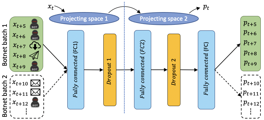
Figure 3. FNN architecture.

We focus on binary classification, that is, each sample can be predicted to be either benign or malicious. We consider two datasets, so we devise a total of four models, i.e., one FNN and one LSTM per dataset. We report in Table 2, the partitioning of the training and testing sets. We use the first $70\%$ of each scenario for training and the remaining for testing (to avoid temporal bias (Pendlebury et al., 2019)); the only exceptions are some scenarios of CICIDS2017, where we must resort to different splits to ensure at that at least $70\%$ of the malicious NetFlows are put in the training set. We remark that both the LSTM and FNN are trained on the same training data, and tested on the same test data. Note also that we keep the Benign1-2 scenarios of CICIDS2017 only for training the models.

5. Evaluation and Results

The goal of the experiments is verifying the existence and effectiveness of the temporal patterns extracted with the proposed method; we do not want to propose a superior technique. Hence, we train the LSTM and FNN on each dataset (as described in Section 4.2), and we perform two types of experiments, which we briefly outline.

Direct comparison. Here, the focus is studying the classification patterns learned by the two models (LSTM and FNN). We do so by analyzing the results of both models on the same testing set. The idea is that different performance implies different learned patterns used for detection. We present and discuss the results of these experiments in Section 5.1.

Ensemble comparison. To truly verify if the two models (FNN and LSTM) learn different patterns, we create a third ‘ensemble’ model that includes both models. More specifically, we join the FNN with the LSTM model through the logical or. Then, we compare this ensemble (denoted as FNN+LSTM) with the stand-alone LSTM model, and test them on the same test data. The intuition is as follows: if we combine the LSTM with the FNN and the performance matches the performance of the stand-alone LSTM, then it will mean that the FNN and LSTM learn the same detection patterns (and vice versa). These experiments are discussed in Section 5.2.

5.1. Initial Assessment (FNN vs LSTM)

We first compare the performance of the sequential LSTM against the static FNN. We evaluate the two classifiers on every scenario of each dataset. We report the results in Table 3, showing the performance metrics of interest: the F1-score; and the complete confusion matrix, where fp (fn) stands for false positives (negatives), and tp (tn) stands for true positives (negatives). We consider a positive as a malicious sample. We split the classification results for each scenario to allow a more fine-grained comparison of the two approaches. The green rows report the aggregated results on the corresponding dataset.

Table 3. Results of the LSTM and FNN on the two datasets.

CICIDS 2017 Scenario F1-score % tp fn tn fp Botnet1 81.755 177 35 45494 44 Botnet2 87.542 130 15 3997 22 Port Scan 99.558 41179 17 46824 349 DDoS 99.572 22588 0 39100 194 DoS GoldenEye 99.707 2384 0 24442 14 DoS Hulk 99.955 58653 17 14322 36 DoS slowhttptest 98.444 1487 40 14220 7 DoS slowloris 99.843 1910 1 8318 5 FTP-Patator 99.600 2866 0 23239 23 SSH-Patator 98.666 2366 0 22708 64 Web Brute Force 99.456 640 0 18181 7 Web XSS 99.153 234 1 6791 3 Long Short-Term Memory Summary 99.669 134614 126 267636 768

CTU 13 Scenario F1-score % tp fn tn fp Menti 95.153 1600 14 26220 149 Murlo 95.640 2369 48 116083 168 Neris1 93.384 8793 468 67235 778 Neris2 90.524 3162 171 46078 491 Neris3 95.911 24901 389 32174 1734 Nsisay 41.445 109 250 14082 58 Rbot1 98.105 14080 249 126574 295 Rbot2 94.873 1101 76 22245 43 Rbot3 99.909 31352 36 48918 21 Rbot4 100.000 3073 0 1500 0 Virut1 87.117 284 22 3439 62 Virut2 80.851 6863 1851 60648 1400 Summary 95.703 97687 3574 565196 5199

Botnet1 93.735 202 10 45521 17 Botnet2 81.569 104 41 4013 6 Port Scan 99.773 41152 44 47030 143 DDoS 99.817 22588 0 39211 83 DoS GoldenEye 99.916 2384 0 24452 4 DoS Hulk 100.000 58670 0 14358 0 DoS slowhttptest 98.303 1477 50 14226 1 DoS slowloris 99.974 1911 0 8322 1 FTP-Patator 99.930 2866 0 23258 4 SSH-Patator 99.705 2366 0 22758 14 Web Brute Force 99.844 640 0 18186 2 Web XSS 99.788 235 0 6793 1 Feedforward Neural Network Summary 99.844 134595 145 268128 276

Menti 84.960 1610 4 25803 566 Murlo 63.267 2413 4 113453 2798 Neris1 85.188 9087 174 65027 2986 Neris2 84.533 3189 144 45546 1023 Neris3 97.353 24605 685 33255 653 Nsisay 44.673 174 185 13894 246 Rbot1 84.926 14299 30 121823 5046 Rbot2 79.619 1170 7 21696 592 Rbot3 98.688 31355 33 48138 801 Rbot4 99.854 3073 0 1491 9 Virut1 75.943 292 14 3330 171 Virut2 87.553 8047 667 60427 1621 Summary 91.497 99314 1947 553883 16512

Let us discuss these results, starting from the CICIDS2017 dataset. By looking at the overall results (green rows), the performance of both LSTM and FNN is similar, and comparable to the state of the art (e.g., (Zhang et al., 2019; Han et al., 2020)). However, by inspecting the performance in the individual scenarios, we can observe some interesting phenomena. Consider the two Botnet scenarios of CICIDS2017 (highlighted in yellow): here, the LSTM learns different classification patterns than the FNN, achieving $81\%$ ($87\%$) F1-score against a $93\%$ ($81\%$) in the Botnet1 (Botnet2) scenario. What is remarkable in these two scenarios is the fact that the malicious samples are from the same botnet type. If we turn the attention to the DoS slowloris and the Port Scan scenarios, the LSTM has almost the same fn of the FNN in the DoS slowloris scenario, but fewer in the Port Scan scenario. These two different types of attacks further highlight that, against some attacks, the LSTM appears to be more effective. The intriguing observation is that a Port Scan typically generates a large volume of (malicious) traffic in a short timeframe; on the contrary, the DoS slowloris generates a small volume of traffic but in long timeframes. Despite these differences, the LSTM seems to adjust its internal time scale (see Section 3.3) for achieving superior performance.

We now focus on the CTU13. Here, on average, both models achieve good performance with over $91\%$ F1-score, in-line with the state of the art (e.g., (Apruzzese et al., 2020)). The LSTM performs better than the FNN in terms of F1-score, and it exhibits a lower amount of fp, but also slightly higher fn, making it a more precise detector for practical purposes. Let us observe the results for the individual scenarios. In the Nsisay scenario both models achieve similar poor performance (below $45\%$ F1-score). The most remarkable differences involve the Neris3 and Virut2 scenarios (highlighted in yellow). In Neris3, the LSTM has a lower number of false-negatives, but it also has a larger number of false-positives; on the other hand, Virut2 is the only scenario where the FNN outperforms the LSTM, and this is clear from the F1-scores of the models. Indeed, the Virut2 scenario is the most ‘problematic’ scenario for the LSTM due to the huge fn. However, everywhere else the LSTM learns different classification patterns that produce superior detection results.

Takeaway: the different performance in the individual scenarios on both datasets may suggest that the LSTM learns different classification patterns than the FNN. Hence, for some specific attacks, the application of the proposed method (and its usage for LSTM-detectors) may yield better NIDS.

5.2. Verification (FNN+LSTM vs LSTM)

Despite the differences shown in the previous experiments, we still cannot be truly sure that the LSTM and FNN have learned different patterns for their classification. As an example, consider the case of Botnet1 in the CICIDS2017 dataset: the FNN has 10 fn, while the LSTM has 35 fn. The question is: are these 10 fn by the FNN also included in the 35 fn by the LSTM? If this is true, then the two models will have learned (very) similar classification patterns; on the other hand, if this is not true, then the two models will have learned (arguably) different classification patterns.

To this purpose, we join the LSTM model with the FNN model with the logical or operator to create a new ensemble (FNN+LSTM). More specifically, for a given test-sample as input, the output will be malicious if at least one model of the ensemble makes a malicious classification; conversely, the output will be benign only if both models agree on a benign classification. Such design choice should reduce the number of fn. We do not retrain the models of the ensemble: we simply input a (test) sample to each trained model, and then join the output with the logical or.

We test the LSTM+FNN ensemble on both datasets and report the results in Table 4. For each dataset, the three columns of the FNN+LSTM report the F1-score and the number of fn and fp for each attack scenario; we summarize the overall results in the last row (green row). The two rightmost columns report the difference ($\Delta$) of each performance metric between the FNN+LSTM and the stand-alone LSTM: hence, in the $\pm$fn and $\pm$fp columns, a negative (positive) value means that the ensemble LSTM+FNN is better (worse) than the stand-alone LSTM.

Table 4. Results of the FNN+LSTM ensemble, and comparison ($\Delta$) with the stand-alone LSTM.

CICIDS2017 Testing data FNN+LSTM $\Delta$ Scenario # NetFlows # Mal F1-score % fn fp $\pm$fn $\pm$fp Botnet1 45750 212 89.936 2 45 -33 1 Botnet2 4164 145 91.558 4 22 -11 0 Port Scan 88369 41196 99.556 9 358 -8 9 DDoS 61882 22588 99.572 0 194 0 0 Dos GoldenEye 26840 2384 99.707 0 14 0 0 DoS Hulk 73028 58670 99.969 0 36 -17 0 DoS slowhttptest 15754 1527 99.443 10 7 -30 0 DoS slowloris 10234 1911 99.869 0 5 -1 0 FTP-Patator 26128 2866 99.600 0 23 0 0 SSH-Patator 25138 2366 98.666 0 64 0 0 Web Brute Force 18828 640 99.456 0 7 0 0 Web XSS 7029 235 99.366 0 3 -1 0 Summary 403144 134740 99.703 25 778 -101 10

CTU13 Testing data FNN+LSTM $\Delta$ Scenario # NetFlows # Mal F1-score % fn fp $\pm$fn $\pm$fp Menti 27983 1614 82.688 2 673 -12 524 Murlo 118668 2417 62.562 4 2884 -44 2716 Neris1 77274 9261 84.099 130 3323 -338 2545 Neris2 49902 3333 82.624 33 1355 -138 864 Neris3 59198 25290 95.938 86 2048 -303 314 Nsisay 14499 359 50.228 139 297 -111 239 Rbot1 141198 14329 84.654 11 5180 -238 4885 Rbot2 23465 1177 79.268 7 605 -69 562 Rbot3 80327 31388 98.664 33 816 -3 795 Rbot4 4573 3073 99.854 0 9 0 9 Virut1 3807 306 74.568 4 202 -18 140 Virut2 70762 8714 87.040 148 2403 -1703 1003 Summary 671656 101261 90.803 597 19795 -2977 14596

Let us discuss Table 4, starting from the CICIDS2017 results. Here, we highlight (in yellow) Botnet1 and DoS slowhttptest scenarios because they show the greatest improvement of the FNN+LSTM ensemble over the stand-alone LSTM. In these scenarios, the ensemble has lower fn than the LSTM, and the same fp (only 1 more for the Botnet1). This is possible because the FNN used in the ensemble correctly identifies the malicious NetFlows that are misclassified by the LSTM. We observe an interesting phenomenon in four scenarios, i.e., DoS slowhttptest, Botnet1-2 and Port Scan. The ensemble has not only lower fn than the stand-alone LSTM, but also lower than the stand-alone FNN (see Table 3). This means the ensemble also benefits from the LSTM because it correctly identifies malicious NetFlows misclassified by the FNN.

We now focus on the CTU13. Here, the FNN+LSTM ensemble does better than the stand-alone LSTM in terms of number of false-negatives. However, the latter has a higher F1-score, i.e., $95.703\%$ vs $90.803\%$. This is due to the more conservative nature of the ensemble in detecting malicious events, which may reduce the fn, but may increase the fp. A more in-depth analysis of each scenario outlines that the ensemble reduces the fn in almost all cases. Notably, in Neris1 and Virut2 scenarios (in yellow) the FNN+LSTM ensemble has significantly lower fn than the stand-alone LSTM, but it also has over $2$k more fp. The rationale is that the FNN is better in detecting malicious NetFlows, which benefits the FNN+LSTM ensemble. However, we also observe that the ensemble also benefits from the LSTM. This is clear if we compare the overall number of false-negatives of the FNN+LSTM ensemble with those of the stand-alone FNN (see Table 3): the former has only 597, while the latter has almost four times that amount with 1947.

Takeaway: the LSTM and FNN appear to have learned different classification patterns, confirming that the application of our method to sequential ML models does influence their detection.

6. Conclusions

In this work, we investigate the use of Long Short-Term Memory (LSTM) neural networks to learn temporal patterns among NetFlows as a result of cyber-attacks. We review and highlight the limitations of related work, which has not truly studied the effectiveness of temporal patterns for NetFlow-based NIDS. Hence, we propose an original method that can be used to extract temporal patterns from labelled NetFlow data. We then apply this method to train a ‘sequential’ LSTM classifier, and compare its performance against a ‘static’ Feedforward Neural Network (FNN) to verify if temporal patterns are truly significant for ML-NIDS.

Our evaluation spans over two recent ML-NIDS datasets, CICIDS2017 and CTU13. The results highlight that LSTM achieves comparable ($\sim\!99\%$ F1-score) or better ($95\%$ vs $91\%$ F1-score) performance in detecting malicious NetFlows than the FNN. However, against some specific attacks, the LSTM proves to be significantly better, yielding lower false negatives and lower false positives.

We verify if the proposed method influences the detection by creating an ensemble of the FNN+LSTM models, and compare it against the stand-alone LSTM. This additional set of experiments further confirms that the LSTM and FNN models learn different classification patterns, which translate to different performance that can be exploited to mitigate some types of attacks. Such comparison confirms that, if properly extracted (e.g., with the proposed method and sequential ML-models), temporal patterns can truly be effective at enhancing the performance of ML-NIDS.

Our paper paves the way to more secure and effective NIDS, which rely not only on ‘static’ ML methods, but also by sequential approaches that leverage the underlying relationships among distinct network traffic samples.

Appendix A Appendix A

When preprocessing the datasets, we one-hot encode the categorical features: source/destination ports, the direction and the protocol. The numerical features are normalized in the range $[0,1]$. We grid-search the most optimal parameters of each model, which we report in Table 5).

Table 5. Hyperparameters (CICIDS2017: left; CTU13: right).

parameter	LSTM	FNN	LSTM	FNN
learning rate	0.001	0.001	0.001	0.001
# epochs	30	20	100	100
dropout	0.2	0.3	0.2	0.2
batch size	1	512	1	1024
optimizer	Adam	Adam	Adam	Adam
truncated BPTT window	N/A	N/A	512	N/A
LSTM1 size	256	N/A	256	N/A
LSTM2 size	256	N/A	256	N/A
FC1 size	N/A	256	N/A	512
FC2 size	N/A	256	N/A	512
FC size	2	2	2	2

References

- (1)
- Apruzzese et al. (2020) Giovanni Apruzzese, Mauro Andreolini, Mirco Marchetti, Andrea Venturi, and Michele Colajanni. 2020. Deep reinforcement adversarial learning against botnet evasion attacks. IEEE T. Netw. Serv. Manag. 17, 4 (2020), 1975–1987.
- Apruzzese et al. (2017) Giovanni Apruzzese, Mirco Marchetti, Michele Colajanni, Gabriele Gambigliani Zoccoli, and Alessandro Guido. 2017. Identifying malicious hosts involved in periodic communications. In Proc. IEEE Int. Symp. Netw. Comp. Appl. 1–8.
- Boukhalfa et al. (2020) Alaeddine Boukhalfa, Abderrahim Abdellaoui, Nabil Hmina, and Habiba Chaoui. 2020. LSTM deep learning method for network intrusion detection system. Int. J. Elec. Comp. Eng. 10 (2020).
- Buczak and Guven (2016) Anna L Buczak and Erhan Guven. 2016. A Survey of Data Mining and Machine Learning Methods for Cyber Security Intrusion Detection. IEEE Comm. Surv. Tut. 18, 2 (2016), 1153–1176.
- Chuang and Wu (2019) Po-Jen Chuang and Dong-Ye Wu. 2019. Applying Deep Learning to Balancing Network Intrusion Detection Datasets. In Proc. Int. Conf. Adv. InfoComm. Tech. 213–217.
- Cieslak et al. (2006) DA Cieslak, NV Chawla, and A Striegel. 2006. Combating imbalance in network intrusion datasets. In Proc. IEEE Int. Conf. Granular Comp. 732–737.
- Cisco (2021) Cisco. 2021. IOS NetFlow. Technical Report. https://www.ciscopress.com/articles/article.asp?p=2812391&seqNum=3
- Dey and Salem (2017) Rahul Dey and Fathi M. Salem. 2017. Gate-variants of Gated Recurrent Unit (GRU) neural networks. In Proc. IEEE Int. Midwest Symp. Circ. Syst. 1597–1600.
- Fei and Tan (2018) Hongxiao Fei and Fengyun Tan. 2018. Bidirectional grid long short-term memory (bigridlstm): A method to address context-sensitivity and vanishing gradient. Algorithms 11, 11 (2018), 172.
- Garcia et al. (2014) Sebastian Garcia, Martin Grill, Jan Stiborek, and Alejandro Zunino. 2014. An empirical comparison of botnet detection methods. Elsevier Comp. Secur. 45 (2014), 100–123.
- Gwon et al. (2019) Hyeokmin Gwon, Chungjun Lee, Rakun Keum, and Heeyoul Choi. 2019. Network Intrusion Detection based on LSTM and Feature Embedding. arXiv:1911.11552 (2019).
- Han et al. (2020) Xueying Han, Rongchao Yin, Zhigang Lu, Bo Jiang, Yuling Liu, Song Liu, Chonghua Wang, and Ning Li. 2020. STIDM: A Spatial and Temporal Aware Intrusion Detection Model. In Proc. IEEE Int. Conf. Trust, Secur. Privacy Comp. Commun. 370–377.
- Jindal et al. (2016) Ishan Jindal, Matthew Nokleby, and Xuewen Chen. 2016. Learning deep networks from noisy labels with dropout regularization. In Proc. IEEE Int. Conf. Data Mining. 967–972.
- Khan et al. (2019) Muhammad Ashfaq Khan, Md Karim, Yangwoo Kim, et al. 2019. A scalable and hybrid intrusion detection system based on the convolutional-LSTM network. Symmetry 11, 4 (2019), 583.
- Khraisat et al. (2019) Ansam Khraisat, Iqbal Gondal, Peter Vamplew, and Joarder Kamruzzaman. 2019. Survey of intrusion detection systems: techniques, datasets and challenges. Springer Cybersecurity 2, 1 (2019), 1–22.
- Kim et al. (2020) Jeeyung Kim, Alex Sim, Jinoh Kim, and Kesheng Wu. 2020. Botnet Detection Using Recurrent Variational Autoencoder. arXiv:2004.00234 (2020).
- Liao et al. (2013) Hung-Jen Liao, Chun-Hung Richard Lin, Ying-Chih Lin, and Kuang-Yuan Tung. 2013. Intrusion detection system: A comprehensive review. Elsevier J, Netw, Comp, Appl. 36, 1 (2013), 16–24.
- Mirza and Cosan (2018) Ali H Mirza and Selin Cosan. 2018. Computer network intrusion detection using sequential LSTM neural networks autoencoders. In Proc. IEEE Sign. Proc. Commun. Appl. Conf. 1–4.
- Mishra et al. (2018) Preeti Mishra, Vijay Varadharajan, Uday Tupakula, and Emmanuel S Pilli. 2018. A detailed investigation and analysis of using machine learning techniques for intrusion detection. IEEE Comm. Surv. Tut. 21, 1 (2018), 686–728.
- Pascanu et al. (2013) Razvan Pascanu, Caglar Gulcehre, Kyunghyun Cho, and Yoshua Bengio. 2013. How to construct deep recurrent neural networks. arXiv:1312.6026 (2013).