Enforcing Statistical Orthogonality in Massive MIMO Systems via Covariance Shaping

Abstract

This paper tackles the problem of downlink data transmission in massive multiple-input multiple-output (MIMO) systems where user equipments (UEs) exhibit high spatial correlation and channel estimation is limited by strong pilot contamination. Signal subspace separation among UEs is, in fact, rarely realized in practice and is generally beyond the control of the network designer (as it is dictated by the physical scattering environment). In this context, we propose a novel statistical beamforming technique, referred to as MIMO covariance shaping, that exploits multiple antennas at the UEs and leverages the realistic non-Kronecker structure of massive MIMO channels to target a suitable shaping of the channel statistics performed at the UE-side. To optimize the covariance shaping strategies, we propose a low-complexity block coordinate descent algorithm that is proved to converge to a limit point of the original nonconvex problem. For the two-UE case, this is shown to converge to a stationary point of the original problem. Numerical results illustrate the sum-rate performance gains of the proposed method with respect to spatial multiplexing in scenarios where the spatial selectivity of the base station is not sufficient to separate closely spaced UEs.

Index terms—Covariance shaping, massive MIMO, multi-user MIMO, pilot contamination, statistical beamforming.

I Introduction

Massive multiple-input multiple-output (MIMO) is a multi-antenna technology that has great potential to boost the spectral efficiency (SE) of cellular networks by means of highly directional beamforming and spatial multiplexing of many user equipments (UEs) in the same time-frequency resources. It thus plays a pivotal role in current 5G New Radio (NR) implementations [3, 4, 5] and is expected to maintain this prominence in future wireless generations [6, 7, 8, 9, 10]. The benefits of massive MIMO can be ascribed to the large number of antennas available at the base station (BS), which we denote by $M$. In this context, it is shown in [11] that the achievable SE of downlink/uplink massive MIMO systems is unbounded as $M$ grows large and when minimum mean squared error (MMSE) precoding/combining is adopted at the BS, which can asymptotically remove any interference. However, in presence of a large number of UEs and finite BS antennas, the aforementioned approach might still be limited by interference and must rely on accurate instantaneous channel state information (CSI). In crowded scenarios, such as outdoor events, transport hubs, and stadiums, the channels of closely spaced UEs exhibit high spatial correlation, which hinders the capability of the BS to separate such UEs during both the channel estimation phase and the data transmission phase. Moreover, when the channel coherence time is limited, non-orthogonal pilots might be used across the UEs during the channel estimation phase, which results in strong pilot contamination [12, 13].

To overcome these issues and facilitate the operations in the massive MIMO regime, several works have proposed to leverage statistical CSI [14, 15, 16, 17, 18, 19, 20, 21, 22, 23, 24, 25]. This consists mainly in the channel covariance matrix of each UE, which is essentially dictated by the angle spread spanned by the multipath propagation of the signals impinging on the antenna array. This angle spread is often bounded due to the high spatial resolution of the massive array compared with the limited scattering. As a result, the channel covariance matrices in massive MIMO tend to be low-rank and dominated by few major propagation directions [11, 17, 18]. This particular property can be exploited for several applications such as reducing the feedback overhead in the channel estimation phase [14, 15, 16] and mitigating the interference in the downlink data transmission phase when the UEs exhibit non-overlapping or orthogonal signal subspaces [17, 18]. For example, statistical CSI can be used to precode signals such that their chosen propagation paths do not interfere in average [19, 20]. In this regard, a robust precoding/decoding design based on the average mean squared error (MSE) matrix is derived in [19] under different CSI conditions, whereas [20] provides a lower bound on the ergodic sum rate for the two-UE setting when the UEs are equipped with a single antenna.

There is also a large body of literature focusing on the hybrid precoding problem, where the beamforming applied at the BS is factorized into an inner and an outer precoding matrix [14, 15, 16, 21, 22]. Here, the former is based on instantaneous CSI while the latter depends only on the second-order channel statistics. This results in reduced pilot length required for the instantaneous effective channel estimation and lower computational complexity associated with the inner precoding design. Moreover, in the context of frequency-division duplex (FDD) systems, such a hybrid precoding method can be used to reduce the size of the resulting effective channels by exploiting the near-orthogonality of the angle spreads of different UE groups [14]. In [15], this approach is shown to incur a vanishing loss compared with the case of full CSI when the number of BS antennas grows large, while the same result is obtained in [16] for the case of finite number of BS antennas and suitable UE scheduling. In time-division duplex (TDD) systems, existing works have pointed out how the exploitation of statistical CSI enables efficient pilot reuse across the UEs [23, 24, 25]. In [23], pilot reuse for massive MIMO transmissions over spatially correlated Rayleigh fading channels is proposed when the angle spreads of the UEs with the same pilots are non-overlapping. In [24], the second-order channel statistics are used to precode the pilots, thus reducing the variance of the channel estimation error by a factor that is proportional to the number of UE antennas. A robust channel estimation method dealing with scenarios in which the angle spreads of the desired and interfering channels are overlapping is proposed in [25] and exploits channel separability in the power domain [26].

Most of the above works rely on specific structures of the channel covariance matrices of the UEs in terms of rank and degree of separation among signal subspaces. Such properties are determined by the locations of the UEs combined with the surrounding scattering environments, where both these factors are generally beyond the control of the network designer. Indeed, in many practical scenarios, the UEs exhibit high spatial correlation, e.g., when they are not sufficiently far apart. Hence, the condition of non-overlapping or orthogonal signal subspaces is rarely satisfied in practice [11]. Note that, in this setting, the number of BS antennas needed to effectively separate interfering UEs with MMSE precoding/combining increases with their spatial correlation, i.e., as the UEs get closer to each other, and may become impractical in crowded scenarios. Moreover, existing works are often based on the assumption of Kronecker channel model owing to its simple analytical formulation. However, such a model has been shown to be an over-simplification of the true nature of MIMO channels [27].

I-A Contributions

Building on the fact that most future UEs are envisioned to be equipped with a small-to-moderate number of antennas, this paper proposes a novel statistical beamforming technique at the UEs-side, referred to as MIMO covariance shaping. While existing methods assume statistical orthogonality among the UEs as a property given by the physical scattering environment and the Kronecker channel model due to its analytical tractability, MIMO covariance shaping aims at modifying the channel statistics of the UEs with highly overlapping channel covariance matrices in order to enforce signal subspace separation in scenarios where the spatial selectivity of the BS is not sufficient to separate such UEs. The proposed approach consists in preemptively applying a statistical beamforming at the UE-side during both the uplink pilot-aided channel estimation phase and the downlink data transmission phase, and relies uniquely on statistical CSI. In this context, each UE employs its antennas to excite only a subset of all the possible propagation directions towards the BS such that the spatial correlation among the interfering UEs is minimized while preserving enough useful power for effective data transmission. Hence, MIMO covariance shaping is suitable for both pilot decontamination in TDD systems and statistical precoding/combining. Remarkably, the proposed method exploits the realistic non-Kronecker channel structure, which allows to suitably alter the channel statistics perceived at the BS by designing the transceiver at the UE-side. Therefore, it has the unique advantage of turning the generally inconvenient non-Kronecker nature of massive MIMO channels into a benefit. Numerical results show the sum-rate performance gains with respect to a reference scheme employing multiple antennas at the UE for spatial multiplexing in scenarios where the spatial selectivity of the BS is not sufficient to separate UEs with highly overlapping channel covariance matrices and the channel estimation is limited by strong pilot contamination.

The MIMO covariance shaping framework was initially proposed in our prior works [1, 2] and recently used for the minimization of the outage probability in [30]. This work extends the metric proposed in [1] to all pairs of interfering UEs to design a statistical receive beamforming at the UE along with a statistical precoding at the BS. Differently from [30], we argue that MIMO covariance shaping must be adopted for both pilot decontamination during the uplink pilot-aided channel estimation phase and combining during the downlink data transmission phase. By doing so, the BS is able to acquire accurate instantaneous estimates of the effective channels, which are then used for efficient downlink precoding and result in a great enhancement of the network performance.

The contributions of this paper are summarized as follows.

• We present the novel concept of MIMO covariance shaping, which aims at designing a suitable shaping of the channel covariance matrices of the UEs to enforce a full or partial separation of their signal subspaces that would be otherwise highly overlapping.

• We point out that the exploitation of the non-Kronecker nature of massive MIMO channels is crucial to suitably alter the channel statistics perceived at the BS by acting at the UE-side.

• We derive a tractable expression of the ergodic achievable sum rate under MIMO covariance shaping with the objective of characterizing the impact of the proposed framework on the system performance.

• We optimize the covariance shaping strategies by minimizing the variance of the inter-UE interference (as a metric to measure the spatial correlation) among the interfering UEs. To this end, we propose a low-complexity block coordinate descent algorithm that is proved to converge to a limit point of the original nonconvex problem. For the two-UE case, this is shown to converge to a stationary point of the original problem.

• We provide numerical results characterizing several scenarios where MIMO covariance shaping outperforms spatial multiplexing. In particular, a superior sum-rate performance is achieved when the spatial selectivity of the BS is not sufficient to separate UEs exhibiting high spatial correlation and the channel estimation is limited by strong pilot contamination.

Outline. The rest of the paper is structured as follows. Section II introduces the system model for a general multi-UE MIMO downlink system. Section III presents the concept of MIMO covariance shaping. Section IV proposes efficient methods to optimize the covariance shaping vectors. Section V presents numerical results to evaluate the performance of the proposed framework. Finally, Section VI concludes the paper.

Notation. Lowercase and uppercase boldface letters denote vectors and matrices, respectively, whereas $(\cdot)^{\mathrm{T}}$, $(\cdot)^{\mathrm{H}}$, and $(\cdot)^{*}$ are the transpose, Hermitian transpose, and conjugate operators, respectively. $\|\cdot\|$ and $\|\cdot\|_{\mathrm{F}}$ represent the Euclidean norm for vectors and the Frobenius norm for matrices, respectively, whereas $\mathbb{E}[\cdot]$ and $\mathbb{V}[\cdot]$ are the expectation and variance operators, respectively. $\mathbf{I}_{A}$ denotes the $A$-dimensional identity matrix and $\mathbf{0}$ represents the zero vector or matrix with proper dimension. $\mathrm{tr}(\cdot)$ and $\mathrm{vec}(\cdot)$ are the trace and vectorization operators, respectively. $(a_{mn})_{m,n=1}^{M}$ denotes the matrix of size $M\times M$ whose $(m,n)$th element is given by $a_{mn}$, whereas $[a_{1},\ldots,a_{A}]$ represents horizontal concatenation. We use $\otimes$ to denote the Kronecker product and $\mathbf{u}_{\min}[\mathbf{A}]$ to denote the eigenvector corresponding to the minimum eigenvalue of matrix $\mathbf{A}$, with $\big{\|}\mathbf{u}_{\min}(\mathbf{A})\big{\|}=1$. $\mathbbm{1}_{A}$ denotes the indicator function, which is equal to $1$ if condition $A$ is satisfied and to $0$ otherwise, and $\lceil\cdot\rceil$ is the ceiling operator. Lastly, $\mathcal{C}\mathcal{N}(\mathbf{0},\mathbf{A})$ is the circularly symmetric complex Gaussian distribution with zero mean and covariance matrix $\mathbf{A}$.

II System Model

In this section, we introduce the channel model for a general multi-UE MIMO downlink system. Then, we describe the uplink pilot-aided channel estimation assuming a TDD setting and channel reciprocity between the uplink and the downlink. Finally, we discuss the system model for the downlink data transmission.

II-A Channel Model

Consider a multi-UE MIMO system where a BS equipped with $M$ antennas serves $K$ UEs with $N$ antennas each in the downlink. Let $\mathbf{H}_{k}\triangleq[\mathbf{h}_{k,1},\ldots,\mathbf{h}_{k,M}]=[\mathbf{g}_{k,1}^{\mathrm{T}},\ldots,\mathbf{g}_{k,N}^{\mathrm{T}}]^{\mathrm{T}}\in\mbox{$\mathbb{C}$}^{N\times M}$ denote the downlink channel matrix of UE $k$, where $\mathbf{h}_{k,m}\in\mbox{$\mathbb{C}$}^{N\times 1}$ and $\mathbf{g}_{k,n}\in\mbox{$\mathbb{C}$}^{1\times M}$ are the channel vectors between the $m$th BS antenna and UE $k$ and between the BS and the $n$th antenna of UE $k$, respectively. We assume a correlated Rayleigh fading channel model where the entries of $\mathbf{H}_{k}$ satisfy $\mathrm{vec}(\mathbf{H}_{k})\sim\mathcal{C}\mathcal{N}(\mathbf{0},\mathbf{\Sigma}_{k})$ [31, Ch. 3]. Here, the channel covariance matrix $\mathbf{\Sigma}_{k}\in\mbox{$\mathbb{C}$}^{NM\times NM}$ has the following general structure:

$$\mathbf{\Sigma}_{k}\triangleq\begin{bmatrix}\mathbf{\Sigma}_{k,11}&\mathbf{\Sigma}_{k,12}&\ldots&\mathbf{\Sigma}_{k,1M}\\ \mathbf{\Sigma}_{k,12}^{\mathrm{H}}&\mathbf{\Sigma}_{k,22}&&\vdots\\ \vdots&&\ddots&\\ \mathbf{\Sigma}_{k,1M}^{\mathrm{H}}&\ldots&&\mathbf{\Sigma}_{k,MM}\end{bmatrix}$$ (1)

where each block $\mathbf{\Sigma}_{k,mn}\triangleq\mathbb{E}[\mathbf{h}_{k,m}\mathbf{h}_{k,n}^{\mathrm{H}}]\in\mbox{$\mathbb{C}$}^{N\times N}$ represents the cross-covariance matrix between the $m$th and $n$th columns of $\mathbf{H}_{k}$. Lastly, we define the covariance matrix seen at UE $k$ as $\mathbf{R}_{k}\triangleq\mathbb{E}[\mathbf{H}_{k}\mathbf{H}_{k}^{\mathrm{H}}]\in\mbox{$\mathbb{C}$}^{N\times N}$ and the covariance matrix relative to UE $k$ seen at the BS as $\mathbf{T}_{k}\triangleq\mathbb{E}[\mathbf{H}_{k}^{\mathrm{H}}\mathbf{H}_{k}]\in\mbox{$\mathbb{C}$}^{M\times M}$, respectively. Observe that, in the case of downlink data transmission, $\mathbf{R}_{k}$ and $\mathbf{T}_{k}$ represent the receive and transmit covariance matrices, respectively.

II-B Uplink Pilot-Aided Channel Estimation

Assuming a TDD setting and channel reciprocity between the uplink and the downlink (see, e.g., [32, Ch. 1.3.5]), the channel matrices $\{\mathbf{H}_{k}\}_{k=1}^{K}$ are estimated at the BS using antenna-specific uplink pilots, such that $N$ pilot vectors per UE are required. Let $\mathcal{S}_{p}\triangleq\{k:\textrm{UE}~{}k~{}\textrm{has~{}pilot}~{}\mathbf{P}_{p}\}$ be the set of UEs sharing the same pilot matrix $\mathbf{P}_{p}\in\mbox{$\mathbb{C}$}^{N\times\tau}$, with $p=1,\ldots,P$. Here, $P<K$ denotes the number of orthogonal pilot matrices and $\tau$ represents the pilot length. The orthogonal pilot matrices satisfy $\{\mathbf{P}_{p}\mathbf{P}_{p}^{\mathrm{H}}=\frac{\tau}{N}\mathbf{I}_{N}\}_{p=1}^{P}$, i.e., $N$ orthogonal pilot vectors are assigned to each UE, and $\{\mathbf{P}_{p}\mathbf{P}_{q}^{\mathrm{H}}=\mathbf{0}\}_{p\neq q}.$ Note that these conditions imply $\tau\geq PN$. Furthermore, $\mathbf{Y}\in\mbox{$\mathbb{C}$}^{M\times\tau}$ denotes the receive signal at the BS during the uplink pilot-aided channel estimation phase, which is given by

$$\mathbf{Y}\triangleq\sum_{p=1}^{P}\sum_{k\in\mathcal{S}_{p}}\sqrt{\rho_{\textnormal{\tiny{UE}}}}\mathbf{H}_{k}^{\mathrm{H}}\mathbf{P}_{p}+\mathbf{Z}$$ (2)

where $\rho_{\textnormal{\tiny{UE}}}$ is the transmit power at the UEs and $\mathbf{Z}\in\mbox{$\mathbb{C}$}^{M\times\tau}$ is the noise term at the BS with elements independently distributed as $\mathcal{C}\mathcal{N}(0,\sigma_{\textnormal{\tiny{BS}}}^{2})$. Let $\mathbf{\Phi}_{k,nn}\triangleq\mathbb{E}[\mathbf{g}_{k,n}^{\mathrm{T}}\mathbf{g}_{k,n}^{*}]\in\mbox{$\mathbb{C}$}^{M\times M}$ denote the covariance matrix of $\mathbf{g}_{k,n}$. Then, the MMSE estimate of $\mathbf{g}_{k,n}$, with $k\in\mathcal{S}_{p}$, is given by (see, e.g., [32, Ch. 3.2])

$$\hat{\mathbf{g}}_{k,n}^{\mathrm{H}}\triangleq\frac{N}{\tau\sqrt{\rho_{\textnormal{\tiny{UE}}}}}\mathbf{\Phi}_{k,nn}\mathbf{Q}_{k,nn}^{-1}\mathbf{Y}\mathbf{P}_{p}^{\mathrm{H}}\mathbf{e}_{n}\in\mbox{$\mathbb{C}$}^{M\times 1}$$ (3)

where $\mathbf{e}_{n}\in\mbox{$\mathbb{R}$}^{N\times 1}$ is the $n$th column of $\mathbf{I}_{N}$, $\mathbf{Q}_{k,nn}\triangleq\big{(}\mathbf{\Phi}_{k,nn}+\sum_{j\in\mathcal{S}_{p}\setminus\{k\}}\mathbf{\Phi}_{j,nn}+\frac{N}{\tau\varrho_{\textnormal{\tiny{UE}}}}\mathbf{I}_{M}\big{)}\in\mbox{$\mathbb{C}$}^{M\times M}$ is the normalized covariance matrix of the receive signal after correlation with $\mathbf{P}_{p}^{\mathrm{H}}\mathbf{e}_{n}$, and $\varrho_{\textnormal{\tiny{UE}}}\triangleq\frac{\rho_{\textnormal{\tiny{UE}}}}{\sigma_{\textnormal{\tiny{BS}}}^{2}}$. Note that (3) can be seen as a superposition of channels estimated using the same pilot $\mathbf{P}_{p}^{\mathrm{H}}\mathbf{e}_{n}$, which cannot be distinguished by the BS: this phenomenon is referred to as pilot contamination [12]. Finally, the MMSE estimate of $\mathbf{H}_{k}$ is obtained as $\hat{\mathbf{H}}_{k}\triangleq[\hat{\mathbf{g}}_{k,1}^{\mathrm{T}},\ldots,\hat{\mathbf{g}}_{k,N}^{\mathrm{T}}]^{\mathrm{T}}\in\mbox{$\mathbb{C}$}^{N\times M}$.

II-C Downlink Data Transmission

In the following, we focus on the downlink data transmission and assume that the BS transmits $L_{k}\leq N$ independent symbols to UE $k$. We denote the transmit symbol vector for UE $k$ by $\mathbf{s}_{k}\in\mbox{$\mathbb{C}$}^{L_{k}\times 1}$, with $\mathbb{E}[\mathbf{s}_{k}\mathbf{s}_{k}^{\mathrm{H}}]=\mathbf{I}_{L_{k}}$, and introduce the multi-UE transmit symbol vector $\mathbf{s}\triangleq[\mathbf{s}_{1}^{\mathrm{T}},\ldots,\mathbf{s}_{K}^{\mathrm{T}}]^{\mathrm{T}}\in\mbox{$\mathbb{C}$}^{L\times 1},$ with $L\triangleq\sum_{k=1}^{K}L_{k}$. Before the transmission, the BS precodes $\mathbf{s}$ using the multi-UE precoding matrix $\mathbf{W}\triangleq[\mathbf{W}_{1},\ldots,\mathbf{W}_{K}]\in\mbox{$\mathbb{C}$}^{M\times L},$ where $\mathbf{W}_{k}\triangleq[\mathbf{w}_{k,1},\ldots,\mathbf{w}_{k,L_{k}}]\in\mbox{$\mathbb{C}$}^{M\times L_{k}}$ is the precoding matrix corresponding to $\mathbf{s}_{k}$ and $\mathbf{W}$ satisfies the power constrain $\|\mathbf{W}\|_{\mathrm{F}}^{2}=1$. The receive signal at UE $k$ is thus given by

$$\mathbf{y}_{k} \triangleq\sqrt{\rho_{\textnormal{\tiny{BS}}}}\mathbf{H}_{k}\mathbf{W}_{k}\mathbf{s}_{k}+\sqrt{\rho_{\textnormal{\tiny{BS}}}}\sum_{j\neq k}\mathbf{H}_{k}\mathbf{W}_{j}\mathbf{s}_{j}+\mathbf{z}_{k}\in\mbox{$\mathbb{C}$}^{N\times 1}$$ (4)

where $\rho_{\textnormal{\tiny{BS}}}$ is the transmit power at the BS and $\mathbf{z}_{k}\sim\mathcal{C}\mathcal{N}(0,\sigma_{\textnormal{\tiny{UE}}}^{2}\mathbf{I}_{N})$ is the noise term at the UEs. Finally, UE $k$ decodes $\mathbf{s}_{k}$ as $\hat{\mathbf{s}}_{k}\triangleq\mathbf{V}_{k}^{\mathrm{H}}\mathbf{y}_{k}\in\mbox{$\mathbb{C}$}^{L_{k}\times 1}$, where $\mathbf{V}_{k}\triangleq[\mathbf{v}_{k,1},\ldots,\mathbf{v}_{k,L_{k}}]\in\mbox{$\mathbb{C}$}^{N\times L_{k}}$ is the corresponding combining matrix. Assuming perfect CSI at the UEs, the resulting sum rate is given by

$$\!R\!\triangleq\!\sum_{k=1}^{K}\!\sum_{\ell=1}^{L_{k}}\log_{2}\!\bigg{(}\!1\!+\!\frac{|\mathbf{v}_{k,\ell}^{\mathrm{H}}\mathbf{H}_{k}\mathbf{w}_{k,\ell}|^{2}}{\sum_{(j,s)\neq(k,\ell)}\!|\mathbf{v}_{k,\ell}^{\mathrm{H}}\mathbf{H}_{k}\mathbf{w}_{j,s}|^{2}\!+\!\frac{1}{\varrho_{\textnormal{\tiny{BS}}}}\|\mathbf{v}_{k,\ell}\|^{2}}\!\bigg{)}$$ (5)

with $\varrho_{\textnormal{\tiny{BS}}}\triangleq\frac{\rho_{\textnormal{\tiny{BS}}}}{\sigma_{\textnormal{\tiny{UE}}}^{2}}$.

III Covariance Shaping at the UE-Side

Although MMSE precoding/combining can asymptotically remove any interference as $M$ grows large [11], this no longer holds in the presence of a large number of UEs and finite BS antennas. In particular, the number of BS antennas needed to effectively separate interfering UEs with MMSE precoding/combining increases with their spatial correlation, i.e., as the UEs get closer to each other, and may become impractical in crowded scenarios. In this setting, the BS can spatially separate signals corresponding to different UEs and mitigate or eliminate pilot contamination if their channel covariance matrices lie on orthogonal supports, i.e., if $\mathbf{\Sigma}_{k}\mathbf{\Sigma}_{j}=\mathbf{0}$ for a given pair of UEs $k$ and $j$ (see, e.g., [11]). However, the degree of statistical orthogonality among the UEs is determined by their locations combined with the surrounding scattering environments and both these factors are generally beyond the control of network designers. Hence, signal subspace separation among the UEs rarely occurs in practice.

In this context, we propose a novel method relying uniquely on statistical CSI and referred to as MIMO covariance shaping (or simply covariance shaping), which is applied at the UE-side to enforce the aforementioned signal subspace separation in scenarios where the spatial selectivity of the BS is not sufficient to separate the UEs. While covariance shaping is conceived in such a way that it is agnostic to the operating frequency, we envision its application especially in sub-$6$ GHz frequency bands, where the availability of BS antennas may be limited and further exacerbates the lack of sufficient spatial selectivity. According to covariance shaping, the UEs preemptively apply a statistical beamforming vector, different for each UE, that aims at spatially separating their transmissions, thus drastically reducing both pilot contamination and interference. Here, the original MIMO channel of each UE is transformed into an effective multiple-input single-output (MISO) channel by combining the transmit/receive signal with the corresponding statistical beamforming vector. To this end, the knowledge of the channel covariance matrices of the UEs is required. Although the time scale at which such information must be acquired and used to compute the covariance shaping vectors increases with the mobility of the UEs (or, more generally, as the channel coherence time reduces), this still happens much less frequently than the instantaneous uplink pilot-aided channel estimation. Remarkably, the proposed method exploits the realistic non-Kronecker structure of massive MIMO channels that allows to suitably alter the channel statistics perceived at the BS by acting at the UE-side, thus turning a generally inconvenient model into a benefit.

Let $\mathbf{v}_{k}\in\mbox{$\mathbb{C}$}^{N\times 1}$ denote the statistical beamforming vector preemptively applied at UE $k$: in the rest of the paper, we refer to $\mathbf{v}_{k}$ as covariance shaping vector. Hence, the original MIMO channel $\mathbf{H}_{k}$ between the BS and each UE $k$ is transformed into the effective MISO channel $\bar{\mathbf{g}}_{k}\triangleq\mathbf{v}_{k}^{\mathrm{H}}\mathbf{H}_{k}\in\mbox{$\mathbb{C}$}^{1\times M}$. In this setting, it follows that $\bar{\mathbf{g}}_{k}\sim\mathcal{C}\mathcal{N}(\mathbf{0},\bar{\mathbf{\Phi}}_{k})$, where $\bar{\mathbf{\Phi}}_{k}\in\mbox{$\mathbb{C}$}^{M\times M}$ is the effective channel covariance matrix defined as

$$\bar{\mathbf{\Phi}}_{k} \triangleq\mathbb{E}[\bar{\mathbf{g}}_{k}^{\mathrm{T}}\bar{\mathbf{g}}_{k}^{*}]$$ (6)

$$=\big{(}(\mathbf{I}_{M}\otimes\mathbf{v}_{k}^{\mathrm{H}})\mathbf{\Sigma}_{k}(\mathbf{I}_{M}\otimes\mathbf{v}_{k})\big{)}^{\mathrm{T}}$$ (7)

with $\mathbf{\Sigma}_{k}$ introduced in (1) and where $\mathbb{E}[\|\bar{\mathbf{g}}_{k}\|^{2}]=\mathrm{tr}(\bar{\mathbf{\Phi}}_{k})$. In the rest of this section, we describe how the two phases of uplink pilot-aided channel estimation and downlink data transmission are modified under covariance shaping and we provide a tractable expression of the resulting ergodic achievable sum rate. The optimization of the covariance shaping vectors is discussed in Section IV. For ease of exposition, we focus on the case where covariance shaping is applied to all the UEs in the systems. Nonetheless, the proposed method may be applied to one or more subsets of closely spaced UEs, e.g., those who cannot be effectively separated with MMSE precoding/combining. In this context, UEs adopting covariance shaping and others employing the multiple antennas for spatial multiplexing can be served simultaneously by the BS in a transparent manner.

$$\gamma_{k} =\frac{\mathrm{tr}(\bar{\mathbf{\Phi}}_{k}\mathbf{Q}_{k}^{-1}\bar{\mathbf{\Phi}}_{k})^{2}}{\sum_{j=1}^{K}\mathrm{tr}(\bar{\mathbf{\Phi}}_{k}\bar{\mathbf{\Phi}}_{j}\mathbf{Q}_{j}^{-1}\bar{\mathbf{\Phi}}_{j})+\sum_{j\in\mathcal{S}_{p}\setminus\{k\}}\mathrm{tr}(\bar{\mathbf{\Phi}}_{k}\mathbf{Q}_{j}^{-1}\bar{\mathbf{\Phi}}_{j})^{2}+\frac{1}{\varrho_{\textnormal{\tiny{BS}}}}\|\mathbf{v}_{k}\|^{2}\sum_{j=1}^{K}\mathrm{tr}(\bar{\mathbf{\Phi}}_{j})}$$ (16)

III-A Uplink Pilot-Aided Channel Estimation

To estimate the effective channels $\{\bar{\mathbf{g}}_{k}\}_{k=1}^{K}$ resulting from covariance shaping, the BS assigns the same pilot vector $\mathbf{p}_{p}\in\mbox{$\mathbb{C}$}^{1\times\tau}$ to all UEs $k\in\mathcal{S}_{p}$, with $\{\|\mathbf{p}_{p}\|^{2}=\tau\}_{p=1}^{P}$ and $\{\mathbf{p}_{p}\mathbf{p}_{q}^{\mathrm{H}}=0\}_{p\neq q}$. The receive signal at the BS during the uplink pilot-aided channel estimation phase, which we denote by $\bar{\mathbf{Y}}\in\mbox{$\mathbb{C}$}^{M\times\tau}$, is given by (cf. (2))

$$\bar{\mathbf{Y}}\triangleq\sum_{p=1}^{P}\sum_{k\in\mathcal{S}_{p}}\sqrt{\rho_{\textnormal{\tiny{UE}}}}\bar{\mathbf{g}}_{k}^{\mathrm{H}}\mathbf{p}_{p}+\mathbf{Z}.$$ (8)

Then, the MMSE estimate of $\bar{\mathbf{g}}_{k}$, with $k\in\mathcal{S}_{p}$, is given by (cf. (3))

$$\hat{\bar{\mathbf{g}}}_{k}^{\mathrm{H}}\triangleq\frac{1}{\tau\sqrt{\rho_{\textnormal{\tiny{UE}}}}}\bar{\mathbf{\Phi}}_{k}\mathbf{Q}_{k}^{-1}\bar{\mathbf{Y}}\mathbf{p}_{p}^{\mathrm{H}}\in\mbox{$\mathbb{C}$}^{M\times 1}$$ (9)

where $\mathbf{Q}_{k}\triangleq\bar{\mathbf{\Phi}}_{k}+\sum_{j\in\mathcal{S}_{p}\setminus\{k\}}\bar{\mathbf{\Phi}}_{j}+\frac{1}{\tau\varrho_{\textnormal{\tiny{UE}}}}\mathbf{I}_{M}\in\mbox{$\mathbb{C}$}^{M\times M}$ is the normalized covariance matrix of the receive signal after correlation with $\mathbf{p}_{p}^{\mathrm{H}}$. Note that the estimation of the effective channels only requires one pilot vector per UE. Hence, the application of covariance shaping can potentially reduce the pilot length with respect to the estimation of the channel matrices $\{\mathbf{H}_{k}\}_{k=1}^{K}$ described in Section II-B, which requires $N$ pilot vectors per UE.

III-B Downlink Data Transmission

Focusing on the downlink data transmission, the BS now transmits only one symbol $s_{k}\in\mbox{$\mathbb{C}$}$ to each UE $k$, i.e., $\{L_{k}=1\}_{k=1}^{K}$. Hence, we have $\mathbf{s}=[s_{1},\ldots,s_{K}]^{\mathrm{T}}\in\mbox{$\mathbb{C}$}^{K\times 1}$ and the multi-UE precoding matrix becomes $\mathbf{W}=[\mathbf{w}_{1},\ldots,\mathbf{w}_{K}]\in\mbox{$\mathbb{C}$}^{M\times K}$, where $\mathbf{w}_{k}\in\mbox{$\mathbb{C}$}^{M\times 1}$ is the precoding vector corresponding to $s_{k}$. The receive signal at UE $k$ is thus given by (cf. (4))

$$\bar{y}_{k} \triangleq\sqrt{\rho_{\textnormal{\tiny{BS}}}}\bar{\mathbf{g}}_{k}\mathbf{w}_{k}s_{k}+\sqrt{\rho_{\textnormal{\tiny{BS}}}}\sum_{j\neq k}\bar{\mathbf{g}}_{k}\mathbf{w}_{j}s_{j}+\mathbf{v}_{k}^{\mathrm{H}}\mathbf{z}_{k}\in\mbox{$\mathbb{C}$}$$ (10)

and, assuming perfect CSI at the UEs, the resulting sum rate is given by (cf. (5))

$$\bar{R}\triangleq\sum_{k=1}^{K}\log_{2}\bigg{(}1+\frac{|\bar{\mathbf{g}}_{k}\mathbf{w}_{k}|^{2}}{\sum_{j\neq k}|\bar{\mathbf{g}}_{k}\mathbf{w}_{j}|^{2}+\frac{1}{\varrho_{\textnormal{\tiny{BS}}}}\|\mathbf{v}_{k}\|^{2}}\bigg{)}.$$ (11)

III-C Ergodic Achievable Sum Rate

We now analyze the sum rate as a function of the covariance shaping vectors with the objective of characterizing the impact of the proposed framework on the system performance. In particular, we derive a tractable expression of the ergodic achievable sum rate by assuming that each UE $k$ does not know the effective scalar channel $\bar{\mathbf{g}}_{k}\mathbf{w}_{k}=\mathbf{v}_{k}^{\mathrm{H}}\mathbf{H}_{k}\mathbf{w}_{k}$ instantaneously but only its expected value. Building on [32, Thm. 4.6], we can express the receive signal in (10) as

$$\bar{y}_{k} =\sqrt{\rho_{\textnormal{\tiny{BS}}}}\mathbb{E}[\bar{\mathbf{g}}_{k}\mathbf{w}_{k}]s_{k}+z_{k}^{\prime}$$ (12)

where the effective noise term $z_{k}^{\prime}\triangleq\sqrt{\rho_{\textnormal{\tiny{BS}}}}\big{(}\bar{\mathbf{g}}_{k}\mathbf{w}_{k}-\mathbb{E}[\bar{\mathbf{g}}_{k}\mathbf{w}_{k}]\big{)}s_{k}+\sqrt{\rho_{\textnormal{\tiny{BS}}}}\sum_{j\neq k}\bar{\mathbf{g}}_{k}\mathbf{w}_{j}s_{j}+\mathbf{v}_{k}^{\mathrm{H}}\mathbf{z}_{k}$ accounts for the lack of instantaneous CSI in addition to the interference and the noise at UE $k$. A lower bound on the signal-to-interference-plus-noise ratio (SINR) achievable by UE $k$ can be obtained by treating $z_{k}^{\prime}$ as Gaussian noise, which yields the effective SINR

$$\gamma_{k} \triangleq\frac{\big{|}\mathbb{E}[\bar{\mathbf{g}}_{k}\mathbf{w}_{k}]\big{|}^{2}}{\mathbb{V}[\bar{\mathbf{g}}_{k}\mathbf{w}_{k}]+\sum_{j\neq k}\mathbb{E}\big{[}|\bar{\mathbf{g}}_{k}\mathbf{w}_{j}|^{2}\big{]}+\frac{1}{\varrho_{\textnormal{\tiny{BS}}}}\|\mathbf{v}_{k}\|^{2}}.$$ (13)

The expression in (13) can be further simplified by considering the case where the BS adopts maximum ratio transmission (MRT) precoding. In this setting, the multi-UE precoding matrix can be written as

$$\mathbf{W}=\frac{\hat{\bar{\mathbf{H}}}^{\mathrm{H}}}{\sqrt{\mathbb{E}[\|\bar{\mathbf{H}}\|_{\mathrm{F}}^{2}]}}$$ (14)

where $\bar{\mathbf{H}}\!\triangleq\![\bar{\mathbf{g}}_{1}^{\mathrm{T}},\ldots,\bar{\mathbf{g}}_{K}^{\mathrm{T}}]^{\mathrm{T}}\!\in\!\mbox{$\mathbb{C}$}^{K\times M}$ and $\hat{\bar{\mathbf{H}}}\!\triangleq\![\hat{\bar{\mathbf{g}}}_{1}^{\mathrm{T}},\ldots,\hat{\bar{\mathbf{g}}}_{K}^{\mathrm{T}}]^{\mathrm{T}}\!\in\!\mbox{$\mathbb{C}$}^{K\times M}$ contain the effective channels and their MMSE estimates defined in (9), respectively. Hence, when MRT precoding is adopted at the BS, the effective SINR of UE $k$ in (13), with $k\in\mathcal{S}_{p}$, reduces to

$$\gamma_{k} =\frac{\big{|}\mathbb{E}[\bar{\mathbf{g}}_{k}\hat{\bar{\mathbf{g}}}_{k}^{\mathrm{H}}]\big{|}^{2}}{\mathbb{V}[\bar{\mathbf{g}}_{k}\hat{\bar{\mathbf{g}}}_{k}^{\mathrm{H}}]+\sum_{j\neq k}\mathbb{E}\big{[}|\bar{\mathbf{g}}_{k}\hat{\bar{\mathbf{g}}}_{j}^{\mathrm{H}}|^{2}\big{]}+\frac{1}{\varrho_{\textnormal{\tiny{BS}}}}\|\mathbf{v}_{k}\|^{2}\mathbb{E}\big{[}\|\bar{\mathbf{H}}\|_{\mathrm{F}}^{2}\big{]}}.$$ (15)

This can be rewritten in closed form as in (16), shown at the top of this page, by substituting the following terms: $\mathbb{E}[\bar{\mathbf{g}}_{k}\hat{\bar{\mathbf{g}}}_{k}^{\mathrm{H}}]=\mathrm{tr}(\bar{\mathbf{\Phi}}_{k}\mathbf{Q}_{k}^{-1}\bar{\mathbf{\Phi}}_{k})$, $\mathbb{V}[\bar{\mathbf{g}}_{k}\hat{\bar{\mathbf{g}}}_{k}^{\mathrm{H}}]=\mathrm{tr}(\bar{\mathbf{\Phi}}_{k}^{2}\mathbf{Q}_{k}^{-1}\bar{\mathbf{\Phi}}_{k})$, $\mathbb{E}\big{[}|\bar{\mathbf{g}}_{k}\hat{\bar{\mathbf{g}}}_{j}^{\mathrm{H}}|^{2}\big{]}=\mathrm{tr}(\bar{\mathbf{\Phi}}_{k}\bar{\mathbf{\Phi}}_{j}\mathbf{Q}_{j}^{-1}\bar{\mathbf{\Phi}}_{j})+\mathbbm{1}_{j\in\mathcal{S}_{p}}\mathrm{tr}(\bar{\mathbf{\Phi}}_{k}\mathbf{Q}_{j}^{-1}\bar{\mathbf{\Phi}}_{j})^{2}$, and $\mathbb{E}\big{[}\|\bar{\mathbf{H}}\|_{\mathrm{F}}^{2}\big{]}=\sum_{k=1}^{K}\mathrm{tr}(\bar{\mathbf{\Phi}}_{k})$. We refer to Appendix A for the detailed derivations. Note that, in the case of perfect channel estimation, i.e., when $\varrho_{\textnormal{\tiny{UE}}}\to\infty$ and all the UEs have orthogonal pilots, we have $\{\bar{\mathbf{\Phi}}_{k}\mathbf{Q}_{k}^{-1}\bar{\mathbf{\Phi}}_{k}=\bar{\mathbf{\Phi}}_{k}\}_{k=1}^{K}$ and $\big{\{}\mathbbm{1}_{j\in\mathcal{S}_{p}}=0\big{\}}_{j\neq k}$. In this context, the effective SINR in (16) simplifies as

$$\gamma_{k} =\frac{\mathrm{tr}(\bar{\mathbf{\Phi}}_{k})^{2}}{\sum_{j=1}^{K}\mathrm{tr}(\bar{\mathbf{\Phi}}_{k}\bar{\mathbf{\Phi}}_{j})+\frac{1}{\varrho_{\textnormal{\tiny{BS}}}}\|\mathbf{v}_{k}\|^{2}\sum_{j=1}^{K}\mathrm{tr}(\bar{\mathbf{\Phi}}_{j})}.$$ (17)

Finally, Proposition 1 presents an ergodic achievable sum rate with MRT in the two cases of perfect and imperfect channel estimation. The proof follows from [32, Thm. 4.6] and is thus omitted.

Proposition 1.

Assume that the BS adopts MRT precoding. Then, an ergodic achievable sum rate is given by

$$\bar{R}^{\rm{lb}}=\sum_{k=1}^{K}\log_{2}(1+\gamma_{k})$$ (18)

with $\gamma_{k}$ defined in (16) and in (17) for imperfect and perfect channel estimation, respectively. Furthermore, the following limit holds as $M\to\infty$:

$$\lim_{M\to\infty}\bar{R}^{\rm{lb}}=\mathbb{E}[\bar{R}]$$ (19)

with $\bar{R}$ defined in (11).

IV Covariance Shaping Optimization

In this section, we address the sum rate maximization through a proper design of the covariance shaping vectors at the UEs. To this end, we consider the variance of the inter-UE interference as a metric to measure the spatial correlation or, in other words, the degree of statistical orthogonality, between two interfering UEs. In the following, we first consider the simple case of $K=2$ and then extend the resulting analysis to the general case of $K\geq 2$.

Let us define the inter-UE interference between UEs $k$ and $j$ after applying covariance shaping as

$$\Omega(\mathbf{v}_{k},\mathbf{v}_{j})\triangleq\frac{\bar{\mathbf{g}}_{k}(\mathbf{v}_{k})\bar{\mathbf{g}}_{j}^{\mathrm{H}}(\mathbf{v}_{j})}{\sqrt{\mathbb{E}\big{[}\|\bar{\mathbf{g}}_{k}(\mathbf{v}_{k})\|^{2}\big{]}\mathbb{E}\big{[}\|\bar{\mathbf{g}}_{j}(\mathbf{v}_{j})\|^{2}\big{]}}}$$ (20)

where the notation $\bar{\mathbf{g}}_{k}(\mathbf{v}_{k})$ makes explicit the dependence of the effective channel $\bar{\mathbf{g}}_{k}$ on the corresponding covariance shaping vector $\mathbf{v}_{k}$. The effective channels of UEs $k$ and $j$ yield asymptotic favorable propagation if they satisfy [32, Ch. 2.5.2]

$$\lim_{M\to\infty}\Omega(\mathbf{v}_{k},\mathbf{v}_{j})=0.$$ (21)

For a practical number of BS antennas $M$, a meaningful performance metric is the variance of $\Omega(\mathbf{v}_{k},\mathbf{v}_{j})$, expressed as

$$\delta(\mathbf{v}_{k},\mathbf{v}_{j}) \triangleq\mathbb{V}\big{[}\Omega(\mathbf{v}_{k},\mathbf{v}_{j})\big{]}$$ (22)

$$=\frac{\mathrm{tr}\big{(}\bar{\mathbf{\Phi}}_{k}(\mathbf{v}_{k})\bar{\mathbf{\Phi}}_{j}(\mathbf{v}_{j})\big{)}}{\mathrm{tr}\big{(}\bar{\mathbf{\Phi}}_{k}(\mathbf{v}_{k})\big{)}\mathrm{tr}\big{(}\bar{\mathbf{\Phi}}_{j}(\mathbf{v}_{j})\big{)}}$$ (23)

where the notation $\bar{\mathbf{\Phi}}_{k}(\mathbf{v}_{k})$ makes explicit the dependence of the effective channel covariance matrix $\bar{\mathbf{\Phi}}_{k}$ on the corresponding covariance shaping vector $\mathbf{v}_{k}$. Note that the terms in the numerator and denominator of (23) can be written as

$$\mathrm{tr}\big{(}\bar{\mathbf{\Phi}}_{k}(\mathbf{v}_{k})\bar{\mathbf{\Phi}}_{j}(\mathbf{v}_{j})\big{)} =\sum_{m,n=1}^{M}\mathbf{v}_{k}^{\mathrm{H}}\mathbf{\Sigma}_{k,mn}\mathbf{v}_{k}\mathbf{v}_{j}^{\mathrm{H}}\mathbf{\Sigma}_{j,nm}\mathbf{v}_{j}$$ (24)

$$=\sum_{m,n=1}^{M}\mathbf{v}_{k}^{\mathrm{H}}\mathbf{\Sigma}_{k,mn}\mathbf{v}_{k}\mathbf{v}_{j}^{\mathrm{H}}\mathbf{\Sigma}_{j,mn}^{\mathrm{H}}\mathbf{v}_{j},$$ (25)

$$\mathrm{tr}\big{(}\bar{\mathbf{\Phi}}_{k}(\mathbf{v}_{k})\big{)} =\mathbf{v}_{k}^{\mathrm{H}}\bigg{(}\sum_{m=1}^{M}\mathbf{\Sigma}_{k,mm}\bigg{)}\mathbf{v}_{k}$$ (26)

where we recall that $\mathbf{\Sigma}_{k,mn}$ represents the cross-covariance matrix between the $m$th and $n$th columns of the original channel $\mathbf{H}_{k}$, i.e., before applying covariance shaping, as defined in (1). Observe that $\delta(\mathbf{v}_{k},\mathbf{v}_{j})=0$ implies $\bar{\mathbf{\Phi}}_{k}\bar{\mathbf{\Phi}}_{j}=\mathbf{0}$, i.e., $\bar{\mathbf{\Phi}}_{k}$ and $\bar{\mathbf{\Phi}}_{j}$ lie on orthogonal supports [11]. Indeed, considering the eigenvalue decomposition of the effective channel covariance matrices, which may be written as $\{\bar{\mathbf{\Phi}}_{i}=\mathbf{U}_{i}\mathbf{\Lambda}_{i}\mathbf{U}_{i}^{\mathrm{H}}\}_{i\in\{k,j\}}$, the condition of statistical orthogonality is satisfied if $\mathbf{U}_{k}=\mathbf{U}_{j}$ and $\mathrm{tr}(\mathbf{\Lambda}_{k}\mathbf{\Lambda}_{j})=0,$ which implies the rank deficiency of both $\bar{\mathbf{\Phi}}_{k}$ and $\bar{\mathbf{\Phi}}_{j}$. Clearly, in the general case, this imposes $M^{2}$ conditions whereas only $2N$ variables can be adjusted: this means that the resulting system of equations can be solved when $N\geq\frac{M^{2}}{2}$, which is generally not verified in practice since $M\gg KN$ in massive MIMO scenarios. Hence, since full signal subspace separation can hardly be achieved by simple transceiver design at the UE-side, it is of interest to minimize the spatial correlation between each pair of interfering UEs.

IV-A Two-UE Case

In the two-UE case, i.e., for $K=2$, the covariance shaping vectors of UEs $k$ and $j$ are computed by solving the optimization problem

$$\begin{array}[]{cl}\displaystyle\operatornamewithlimits{minimize}_{\mathbf{v}_{k},\mathbf{v}_{j}}&\displaystyle\delta(\mathbf{v}_{k},\mathbf{v}_{j})\\ \mathrm{subject~{}to}&\displaystyle\|\mathbf{v}_{k}\|^{2}=\|\mathbf{v}_{j}\|^{2}=1\end{array}$$ (29)

with $\delta(\mathbf{v}_{k},\mathbf{v}_{j})$ defined in (23). Although problem (29) is not convex in either $\mathbf{v}_{k}$ or $\mathbf{v}_{j}$, a suboptimal solution can be efficiently obtained via alternating optimization, as suggested in [1]. Let us introduce the definition

$$\eta_{j,mn}(\mathbf{v}_{j})\triangleq\frac{\mathbf{v}_{j}^{\mathrm{H}}\mathbf{\Sigma}_{j,mn}^{\mathrm{H}}\mathbf{v}_{j}}{\mathbf{v}_{j}^{\mathrm{H}}\big{(}\sum_{m=1}^{M}\mathbf{\Sigma}_{j,mm}\big{)}\mathbf{v}_{j}}.$$ (30)

The optimal covariance shaping vector of UE $k$ for a given $\mathbf{v}_{j}$, denoted by $\mathbf{v}_{k}^{\star}$, is obtained as

$$\mathbf{v}_{k}^{\star}=\operatornamewithlimits{argmin}_{\mathbf{v}_{k}\,:\,\|\mathbf{v}_{k}\|^{2}=1}\frac{\sum_{m,n=1}^{M}\mathbf{v}_{k}^{\mathrm{H}}\big{(}\eta_{j,mn}(\mathbf{v}_{j})\mathbf{\Sigma}_{k,mn}\big{)}\mathbf{v}_{k}}{\mathbf{v}_{k}^{\mathrm{H}}\big{(}\sum_{m=1}^{M}\mathbf{\Sigma}_{k,mm}\big{)}\mathbf{v}_{k}}.$$ (31)

Since (31) is in the form of generalized Rayleigh quotient, it admits the solution

$$\mathbf{v}_{k}^{\star}=\mathbf{u}_{\min}\bigg{[}\bigg{(}\sum_{m=1}^{M}\mathbf{\Sigma}_{k,mm}\bigg{)}^{-1}\bigg{(}\sum_{m,n=1}^{M}\eta_{j,mn}(\mathbf{v}_{j})\mathbf{\Sigma}_{k,mn}\bigg{)}\bigg{]}$$ (32)

and the optimal covariance shaping vector of UE $j$ for a given $\mathbf{v}_{k}$ is obtained in a similar way. Hence, problem (29) is solved by alternating the optimization between $\mathbf{v}_{k}$ and $\mathbf{v}_{j}$ until a predetermined convergence criterion is satisfied, e.g., until the difference between the values of the objective in consecutive iterations is sufficiently small. This scheme is formalized in Algorithm 1, whose convergence properties are characterized in Proposition 2.

   Data: $\mathbf{v}_{k}^{(0)}$, $\mathbf{v}_{j}^{(0)}$, $\mathbf{\Sigma}_{k}$, $\mathbf{\Sigma}_{j}$, and the accuracy $\epsilon$. Fix $n=1$.

   While $\big{|}\delta(\mathbf{v}_{k}^{(n)},\mathbf{v}_{j}^{(n)})-\delta(\mathbf{v}_{k}^{(n-1)},\mathbf{v}_{j}^{(n-1)})\big{|}/\delta(\mathbf{v}_{k}^{(n)},\mathbf{v}_{j}^{(n)})>\epsilon$

• Given $\mathbf{v}_{j}^{(n-1)}$, compute $\{\eta_{j,mn}(\mathbf{v}_{j}^{(n-1)})\}_{m,n=1}^{M}$ as in (30).

• Compute $\mathbf{v}_{k}^{(n)}$ as in (32).

• Given $\mathbf{v}_{k}^{(n)}$, compute $\{\eta_{k,mn}(\mathbf{v}_{k}^{(n)})\}_{m,n=1}^{M}$ as in (30).

• Compute $\mathbf{v}_{j}^{(n)}$ as in (32).

   End

• Fix $\mathbf{v}_{k}=\mathbf{v}_{k}^{(n)}$ and $\mathbf{v}_{j}=\mathbf{v}_{j}^{(n)}$.

Algorithm 1 (Covariance shaping: Alternating optimization algorithm)

Proposition 2.

The alternating optimization algorithm described in Algorithm 1 converges to a stationary point of problem (29).

Proof:

Observe that the objective function in (31) does not depend on the scaling of $\mathbf{v}_{k}$ and, if we relax the nonconvex constraint $\|\mathbf{v}_{k}\|^{2}=1$ as $\|\mathbf{v}_{k}\|^{2}\leq 1$, (32) remains a solution of (31). Then, according to [34, Corollary 2], every limit point of the sequence generated by the alternating optimization algorithm applied to problem (29) with the relaxed constraints is a stationary point of the original problem. ∎

Algorithm 1 can be implemented in a centralized manner at the BS and the covariance shaping vectors are fed back to the corresponding UEs. Alternatively, it can be implemented in a distributed fashion at the UEs. In this case, each UE can compute its covariance shaping vector without any information exchange with the other UE provided that the channel statistics of the latter are known, the order of update is fixed, and the same initial points are used. In fact, under these conditions, the entire alternating optimization procedure can be carried out locally and independently at each UE. Note that the same considerations hold for Algorithm 2 presented in the next section for the multi-UE case, where we also discuss the computational complexity.

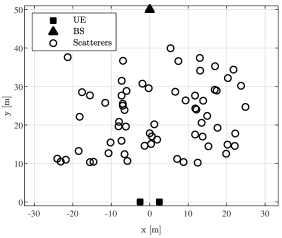
(a) NLoS scenario with $K=2$.

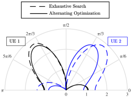
(b) Corresponding covariance shaping vectors.

Figure 1: Two-UE case: (a) 2D map of the considered NLoS scenario with inter-UE distance $d=4$ m; (b) corresponding covariance shaping vectors with $N=2$ obtained with exhaustive search and with Algorithm 1.

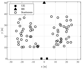
(a) LoS scenario with $K=2$.

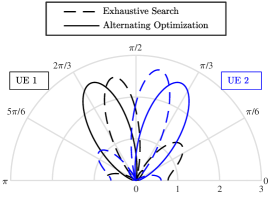
(b) Corresponding covariance shaping vectors.

Figure 2: Two-UE case: (a) 2D map of the considered LoS scenario with inter-UE distance $d=4$ m; (b) corresponding covariance shaping vectors with $N=2$ obtained with exhaustive search and with Algorithm 1.

The result of the covariance shaping optimization heavily depends on the physical scattering environment. Consider the non-line-of-sight (NLoS) scenario in Fig. 1(a), where there is no line-of-sight (LoS) path between the BS and the UEs, the UEs are equipped with uniform linear arrays (ULAs), and the inter-UE distance is $d=4$ m. In this case, as shown in Fig. 1(b), the covariance shaping vectors tend to focus their power along reflected paths that interfere with each other as little as possible while also carrying sufficient channel power, which results in a nearly interference-free transmission/reception. On the other hand, when a LoS path exists, as in the LoS scenario in Fig. 2(a), this generally carries more channel power than any other path. In this case, as shown in Fig. 2(b), the propagation directions selected by the covariance shaping vectors tend to partially capture the LoS path while also focusing some of their power along separated reflected paths in order to achieve some degree of statistical orthogonality between the UEs. Remarkably, in both Fig. 1(b) and Fig. 2(b), the result of Algorithm 1 is very close to the optimal solution of problem (29) obtained with exhaustive search within a set of $10^{3}$ uniformly distributed vectors over the $N$-dimensional unit sphere for each UE, where the former is characterized by negligible complexity with respect to the latter.

Kronecker Channel Model. Let us consider the particular case where each channel $\mathbf{H}_{k}$ follows the Kronecker channel model [28]. In this setting, we have $\mathbf{H}_{k}=\mathbf{R}_{k}^{\frac{1}{2}}\mathbf{H}_{k}^{(\textrm{w})}\mathbf{T}_{k}^{\frac{1}{2}}$, with $\mathbf{R}_{k}$ and $\mathbf{T}_{k}$ defined in Section II and $\mathrm{vec}(\mathbf{H}_{k}^{(\textrm{w})})\sim\mathcal{C}\mathcal{N}(\mathbf{0},\mathbf{I}_{NM})$. Accordingly, the channel covariance matrix in (1) can be expressed as $\mathbf{\Sigma}_{k}=\mathbf{T}_{k}^{\mathrm{T}}\otimes\mathbf{R}_{k}$ with block elements given by $\mathbf{\Sigma}_{k,mn}=T_{k,mn}^{*}\mathbf{R}_{k}$, where $T_{k,mn}$ denotes the $(m,n)$th element of $\mathbf{T}_{k}$. Hence, from (23), we have

$$\delta(\mathbf{v}_{k},\mathbf{v}_{j})$$

$$=\frac{\mathrm{tr}\big{(}(\mathbf{v}_{k}^{\mathrm{H}}\mathbf{\Sigma}_{k,mn}\mathbf{v}_{k})_{m,n=1}^{M}(\mathbf{v}_{j}^{\mathrm{H}}\mathbf{\Sigma}_{j,mn}^{\mathrm{H}}\mathbf{v}_{j})_{m,n=1}^{M}\big{)}}{\mathrm{tr}\big{(}(\mathbf{v}_{k}^{\mathrm{H}}\mathbf{\Sigma}_{k,mn}\mathbf{v}_{k})_{m,n=1}^{M}\big{)}\mathrm{tr}\big{(}(\mathbf{v}_{j}^{\mathrm{H}}\mathbf{\Sigma}_{j,mn}^{\mathrm{H}}\mathbf{v}_{j})_{m,n=1}^{M}\big{)}}$$ (33)

$$=\frac{\mathrm{tr}\big{(}(T_{k,mn}\mathbf{v}_{k}^{\mathrm{H}}\mathbf{R}_{k}\mathbf{v}_{k})_{m,n=1}^{M}(T_{j,mn}\mathbf{v}_{j}^{\mathrm{H}}\mathbf{R}_{j}\mathbf{v}_{j})_{m,n=1}^{M}\big{)}}{\mathrm{tr}\big{(}(T_{k,mn}\mathbf{v}_{k}^{\mathrm{H}}\mathbf{R}_{k}\mathbf{v}_{k})_{m,n=1}^{M}\big{)}\mathrm{tr}\big{(}(T_{j,mn}\mathbf{v}_{j}^{\mathrm{H}}\mathbf{R}_{j}\mathbf{v}_{j})_{m,n=1}^{M}\big{)}}$$ (34)

$$=\frac{\mathrm{tr}(\mathbf{T}_{k}\mathbf{T}_{j})}{\mathrm{tr}(\mathbf{T}_{k})\mathrm{tr}(\mathbf{T}_{j})}.$$ (35)

It is straightforward to observe that, in this case, $\delta(\mathbf{v}_{k},\mathbf{v}_{j})$ is independent of $\mathbf{v}_{k}$ and $\mathbf{v}_{j}$. Hence, under the Kronecker channel model, it is not possible to alter the channel statistics perceived at one end of the communication link by designing the transceiver at the other end: as a consequence, no meaningful effective channel separation can be performed. This is in accordance with the properties of the Kronecker channel model, whereby the transmit and receive covariance matrices are independent. In this context, the signal subspace separation is exclusively determined by the physical scattering environment and can only be achieved when $\mathrm{tr}(\mathbf{T}_{k}\mathbf{T}_{j})=0$, which is rarely satisfied in practice [27, 28].

IV-B Multi-UE Case

In the general case, i.e., for $K\geq 2$, the covariance shaping vectors for each UE are computed by solving the optimization problem

$$\begin{array}[]{cl}\displaystyle\operatornamewithlimits{minimize}_{\{\mathbf{v}_{k}\}_{k=1}^{K}}&\displaystyle\sum_{\begin{subarray}{c}k\neq j\end{subarray}}\delta(\mathbf{v}_{k},\mathbf{v}_{j})\\ \mathrm{subject~{}to}&\displaystyle\big{\{}\|\mathbf{v}_{k}\|^{2}=1\big{\}}_{k=1}^{K}\end{array}$$ (38)

with $\delta(\mathbf{v}_{k},\mathbf{v}_{j})$ defined in (23). Although problem (38) is not convex in any of the optimization variables $\{\mathbf{v}_{k}\}_{k=1}^{K}$, a suboptimal solution can be efficiently obtained via block coordinate descent, which can be interpreted as an extension of the alternating optimization approach presented in the previous section for the two-UE case. The optimal covariance shaping vector of UE $k$ for given $\{\mathbf{v}_{j}\}_{j\neq k}$ is obtained as

$$\mathbf{v}_{k}^{\star}=\operatornamewithlimits{argmin}_{\mathbf{v}_{k}\,:\,\|\mathbf{v}_{k}\|^{2}=1} \frac{\sum_{m,n=1}^{M}\mathbf{v}_{k}^{\mathrm{H}}\big{(}\sum_{j\neq k}\eta_{j,mn}(\mathbf{v}_{j})\mathbf{\Sigma}_{k,mn}\big{)}\mathbf{v}_{k}}{\mathbf{v}_{k}^{\mathrm{H}}\big{(}\sum_{m=1}^{M}\mathbf{\Sigma}_{k,mm}\big{)}\mathbf{v}_{k}}$$ (39)

with $\eta_{j,mn}(\mathbf{v}_{j})$ defined in (30). Like (31), (39) is in the form of generalized Rayleigh quotient and thus admits the solution

$$\mathbf{v}_{k}^{\star}=\mathbf{u}_{\min}\!\bigg{[}\bigg{(}\sum_{m=1}^{M}\mathbf{\Sigma}_{k,mm}\!\bigg{)}^{-1}\!\bigg{(}\sum_{m,n=1}^{M}\sum_{j\neq k}\eta_{j,mn}(\mathbf{v}_{j})\mathbf{\Sigma}_{k,mn}\!\bigg{)}\bigg{]}$$ (40)

and the optimal covariance shaping vectors of the other UEs $j$ for given $\{\mathbf{v}_{k}\}_{k\neq j}$ are obtained in a similar way. Hence, problem (38) is solved by optimizing the strategy of each UE given the strategies of the other UEs until a predetermined convergence criterion is satisfied. Furthermore, at each iteration $i$, the update $\mathbf{v}_{k}^{(i)}=\alpha\mathbf{v}_{k}^{\star}+(1-\alpha)\mathbf{v}_{k}^{(i-1)}$ can be used to limit the variation of the covariance shaping vectors between consecutive iterations, where the step size $\alpha\in(0,1]$ is chosen to strike the proper balance between convergence speed and accuracy (see, e.g., [10, 35]). The proposed scheme is formalized in Algorithm 2, whose convergence properties are characterized in Proposition 3.

Proposition 3.

The block coordinate descent algorithm described in Algorithm 2 converges to a limit point of problem (38).

   Data: $\{\mathbf{v}_{k}^{(0)}\}_{k=1}^{K}$, $\{\mathbf{\Sigma}_{k}\}_{k=1}^{K}$, $\alpha\in(0,1]$, and the accuracy $\epsilon$. Fix $n=1$.

   While

$$\sum_{\begin{subarray}{c}k\neq j\end{subarray}}\frac{\big{|}\delta(\mathbf{v}_{k}^{(n)},\mathbf{v}_{j}^{(n)})-\delta(\mathbf{v}_{k}^{(n-1)},\mathbf{v}_{j}^{(n-1)})\big{|}}{\delta(\mathbf{v}_{k}^{(n)},\mathbf{v}_{j}^{(n)})}>\epsilon$$

  For $k=1,\ldots,K$

• Given $\{\mathbf{v}_{j}^{(n-1)}\}_{j\neq k}$, compute

  $\{\eta_{j,mn}(\mathbf{v}_{j}^{(n)})\}_{m,n=1}^{M}$ as in (30), $\forall j\neq k$.

• Compute $\mathbf{v}_{k}^{\star}$ as in (40).

• Update $\mathbf{v}_{k}^{(n)}=\alpha\mathbf{v}_{k}^{\star}+(1-\alpha)\mathbf{v}_{k}^{(n-1)}$.

  End

   End

• Fix $\{\mathbf{v}_{k}=\mathbf{v}_{k}^{(n)}\}_{k=1}^{K}$.

Algorithm 2 (Covariance shaping: Block coordinate descent algorithm)

Proof:

At each iteration $i$ of Algorithm 1, the covariance shaping vector of UE $k$ results from solving (31), which admits the optimal solution in (32). Hence, the sequence $\big{\{}\delta(\mathbf{v}_{k}^{(i)},\mathbf{v}_{j}^{(i)})\big{\}}_{i}$ is non-increasing since

$$\delta(\mathbf{v}_{k}^{(i)},\mathbf{v}_{j}^{(i-1)})\leq\delta(\mathbf{v}_{k}^{(i-1)},\mathbf{v}_{j}^{(i-1)}).$$ (41)

Moreover, since $\delta(\mathbf{v}_{k},\mathbf{v}_{j})\geq 0$, the sequence $\big{\{}\delta(\mathbf{v}_{k}^{(i)},\mathbf{v}_{j}^{(i)})\big{\}}_{i}$ converges to a finite non-negative value. ∎

The computational complexity of Algorithm 2 is essentially dictated by step S.2, which corresponds to the computation of the optimal covariance shaping vector of UE $k$ for given $\{\mathbf{v}_{j}\}_{j\neq k}$. This is expressed in (40) and has a complexity $\mathcal{O}(N^{2.37})$ due to the eigenvalue decomposition and inverse matrix operations [25]. Hence, the overall computational complexity of Algorithm 2 is $\mathcal{O}(IKN^{2.37})$, where $I$ is the number of iterations required for convergence. Note that both $N$ and $I$ are fairly modest since the UEs are equipped with a small-to-moderate number of antennas and the algorithm converges in very few iterations (i.e., less than $10$ in the simulation scenarios considered in Section V). We can thus conclude that Algorithms 1 and 2 are remarkably efficient in terms of computation complexity.

V Numerical Results and Discussion

In this section, we present numerical results to evaluate the gains achieved by the proposed covariance shaping framework. To this end, we compare the following alternative transmission/reception schemes, where the first is based on covariance shaping and the second is considered as a reference.

• Covariance shaping. The multiple antennas at the UE are employed to implement covariance shaping and one data stream per UE is transmitted using MMSE precoding. Specifically, each UE $k$ applies its covariance shaping vector $\mathbf{v}_{k}$, obtained with Algorithm 1 or Algorithm 2 (depending on the value of $K$), during both the uplink pilot-aided channel estimation phase and the downlink data transmission phase, as discussed in Section IV. The BS obtains the MMSE estimates of the resulting effective channels $\{\bar{\mathbf{g}}_{k}\}_{k=1}^{K}$ as in (9) based on the transmission of $P<K$ orthogonal pilot vectors by the UEs. These estimates are used to compute the $(M\times K)$-dimensional MMSE precoding matrix at the BS as in [11].

• Spatial multiplexing. The multiple antennas at the UE are employed for spatial multiplexing and $N$ data streams per UE are transmitted using MMSE precoding. Specifically, the BS obtains the MMSE estimates of the channel matrices $\{\mathbf{H}_{k}\}_{k=1}^{K}$ as in (3) based on the transmission of $P<K$ orthogonal pilot matrices by the UEs. These estimates are used to compute the $(M\times KN)$-dimensional MMSE precoding matrix at the BS as in [11].

Some comments are in order.

• The reference scheme in (B) requires antenna-specific pilots for the estimation of the channel matrices $\{\mathbf{H}_{k}\}_{k=1}^{K}$. In particular, $N$ orthogonal pilot vectors are assigned to each UE to avoid any pilot contamination among the antennas of the same UE, which implies $\tau\geq PN$. On the other hand, the estimation of the effective channels $\{\bar{\mathbf{g}}_{k}\}_{k=1}^{K}$ resulting from covariance shaping requires $\tau\geq P$ and, therefore, the pilot length can potentially be reduced.

• The reference scheme in (B) allows the transmission of up to $N$ data streams per UE, while only one data stream per UE is transmitted when covariance shaping is used. In the following, we demonstrate how the proposed covariance shaping method can effectively outperform spatial multiplexing in scenarios where the UEs exhibit highly overlapping channel covariance matrices and the spatial selectivity of the BS is not sufficient to separate such UEs.

We evaluate different scenarios in which the BS serves $K$ closely spaced UEs. We assume that the UEs are equipped with ULAs, whereas both ULAs and uniform planar arrays (UPAs) are considered at the BS. In this context, we define the ULA response at each UE for the angle of impingement $\theta$ as

$$\mathbf{a}(\theta) \triangleq[1,e^{-2\pi\delta\cos(\theta)},\ldots,e^{-2\pi\delta(N-1)\cos(\theta)}]^{\mathrm{T}}\in\mbox{$\mathbb{C}$}^{N\times 1}$$ (42)

where $\delta=0.5$ represents the ratio between the antenna spacing and the signal wavelength. Likewise, we define the UPA response at the BS for the angles of impingement $\phi$ along the azimuth direction and $\psi$ along the elevation direction as

$$\mathbf{b}(\phi,\psi)$$

$$\triangleq[1,e^{-2\pi\delta\cos(\phi)},\ldots,e^{-2\pi\delta(M_{x}-1)\cos(\phi)}]^{\mathrm{T}}$$

$$\phantom{=}\ \otimes[1,e^{-2\pi\delta\sin(\psi)},\ldots,e^{-2\pi\delta(M_{y}-1)\sin(\psi)}]^{\mathrm{T}}\in\mbox{$\mathbb{C}$}^{M\times 1}$$ (43)

where $M_{x}$ and $M_{y}$ represent the number of BS antennas along the azimuth and elevation directions, respectively, with $M=M_{x}M_{y}$. The ULA response at the BS for the angle of impingement $\phi$ can be recovered from (43) by setting $M_{x}=M$, $M_{y}=1$, and $\psi=0$. Then, the instantaneous channel between the BS and each UE $k$ follows the discrete physical channel model in [38] and is given by

$$\mathbf{H}_{k} =\sqrt{\frac{\kappa}{1+\kappa}}d_{k}^{-\frac{\beta}{2}}\mathbf{a}(\theta_{k})\mathbf{b}(\phi_{k},\psi_{k})^{\mathrm{H}}$$

$$\phantom{=}\ +\sqrt{\frac{1}{1+\kappa}}\sum_{u=1}^{U}d_{k,u}^{-\frac{\beta}{2}}\alpha_{k,u}\mathbf{a}(\theta_{k,u})\mathbf{b}(\phi_{k,u},\psi_{k,u})^{\mathrm{H}}$$ (44)

where $\kappa$ is the Ricean factor, $U$ is the number of reflected paths, $d_{k}$ and $d_{k,u}$ are the distances of the LoS path and of the $u$th reflected path, respectively, $\theta_{k}$ and $\theta_{k,u}$ are the angles of impingement at the UE of the LoS path and of the $u$th reflected path, respectively, $\phi_{k}$ (resp. $\psi_{k}$) and $\phi_{k,u}$ (resp. $\psi_{k,u}$) are the angles of impingement at the BS of the LoS path and of the $u$th reflected path along the azimuth (resp. elevation) direction, respectively, $\alpha_{k,u}$ is the random phase delay of the $u$th reflected path, and $\beta$ is the pathloss exponent. Unless otherwise stated, we use the simulation parameters listed in Table I. The following results are obtained by means of Monte Carlo simulations with $5\times 10^{3}$ independent channel realizations. Lastly, we point out that, in the considered simulation scenarios, Algorithms 1 and 2 are always observed to converge in very few iterations, i.e., less than $10$.

Parameter		Symbol		Value
Number of BS antennas		$M$		$128$
Number of UEs		$K$		$\{2,4,8\}$
Number of UE antennas		$N$		$2$
Noise variance at the BS		$\sigma_{\textnormal{\tiny{BS}}}^{2}$		$-80$ dBm
Noise variance at the UEs		$\sigma_{\textnormal{\tiny{UE}}}^{2}$		$-80$ dBm
Transmit power at the BS		$\rho_{\textnormal{\tiny{BS}}}$		$30$ dBm
Transmit power at the UEs		$\rho_{\textnormal{\tiny{UE}}}$		$25$ dBm
Number of orthogonal pilots		$P$		$\big{\lceil}\frac{K}{2}\big{\rceil}$
Pilot length		$\tau$		$\{1,2,4\}$
Ricean factor		$\kappa$		$2.5$ (LoS) $0$ (NLoS)
Pathloss exponent		$\beta$		$2$
Inter-UE distance		$d$		$\{2,4\}$ m

TABLE I: Simulation parameters (unless otherwise stated).

V-A Two-UE case

Following the discussion in Section IV-A, we first study the simple case of $K=2$ UEs in order to highlight the key features of the proposed covariance shaping framework. In this setting, we assume $P=1$, i.e., the UEs are assigned the same pilot, and we remark that there is no pilot contamination among the antennas of the same UE for the reference scheme in (B). Assuming that the BS is equipped with a ULA, we consider the LoS and NLoS scenarios illustrated in Fig. 1(a) and in Fig. 2(a), respectively, where the corresponding covariance shaping vectors are shown in Fig. 1(b) and in Fig. 2(b), respectively. Observe that, in both cases, the inter-UE distance is $d=4$ m: this is quite small compared with the distance of about $50$ m between the UEs and the BS, and results in highly overlapping channel covariance matrices.

Let us define the normalized MSE (NMSE) of the channel estimation for UE $k$ as

$$\overline{\mathrm{NMSE}}_{k}\triangleq\mathbb{E}\left[\frac{\|\hat{\bar{\mathbf{g}}}_{k}-\bar{\mathbf{g}}_{k}\|^{2}}{\|\bar{\mathbf{g}}_{k}\|^{2}}\right]$$ (45)

for the effective channels $\{\hat{\bar{\mathbf{g}}}_{k}\}_{k=1}^{K}$ resulting from covariance shaping and as

$$\mathrm{NMSE}_{k}\triangleq\frac{1}{N}\sum_{n=1}^{N}\mathbb{E}\left[\frac{\|\hat{\mathbf{g}}_{k,n}-\mathbf{g}_{k,n}\|^{2}}{\|\mathbf{g}_{k,n}\|^{2}}\right]$$ (46)

for the channel matrices $\{\hat{\mathbf{H}}_{k}\}_{k=1}^{K}$. Considering the NLoS scenario in Fig. 1(a), Fig. 3 plots the NMSE of the channel estimation versus the transmit power at the UEs. Thanks to the improved statistical orthogonality between the UEs, covariance shaping considerably increases the channel estimation accuracy with respect to the case where the original MIMO channels are estimated in the presence of pilot contamination among the antennas of different UEs.

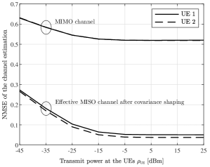
Figure 3: Two-UE case: NMSE of the channel estimation versus the transmit power at the UEs $\rho_{\textnormal{\tiny{UE}}}$ for the NLoS scenario depicted in Fig. 1(a), with ULA at the BS.

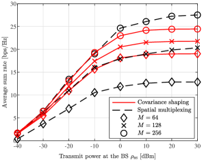
Figure 4: Two-UE case: average sum rate versus the transmit power at the BS $\rho_{\textnormal{\tiny{BS}}}$ for the NLoS scenario depicted in Fig. 1(a), with $d=4$ m, ULA at the BS, and for different values of $M$.

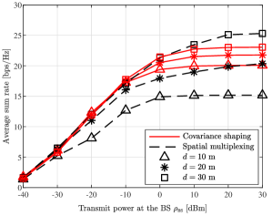
Figure 5: Two-UE case: average sum rate versus the transmit power at the BS $\rho_{\textnormal{\tiny{BS}}}$ for the LoS scenario depicted in Fig. 2(a), with $M=128$, ULA at the BS, and for different values of $d$.

Considering again the NLoS scenario in Fig. 1(a), Fig. 4 plots the average sum rate versus the transmit power at the BS $\rho_{\textnormal{\tiny{BS}}}$ for different numbers of BS antennas $M$. For $M\leq 128$, it is straightforward to see that the signal subspace separation enforced by covariance shaping during both the uplink pilot-aided channel estimation phase and the downlink data transmission phase has a highly beneficial effect on the system performance. However, covariance shaping is outperformed by the reference scheme in (B) for $M=256$. In this setting, the enhanced spatial selectivity of the BS allows to effectively separate the UEs and promotes the transmission of multiple data streams per UE. Focusing now on the LoS scenario in Fig. 2(a), Fig. 5 plots the average sum rate versus the transmit power at the BS $\rho_{\textnormal{\tiny{BS}}}$, with $M=128$ and for different values of the inter-UE distance $d$. Evidently, the reference scheme in (B) is markedly limited by the overlapping channel covariance matrices of the UEs and is able to effectively separate the UEs only for very large inter-UE distances (i.e., $d=30$ m). On the other hand, covariance shaping is able to enforce statistical orthogonality even when the UEs are closely spaced.

V-B Multi-UE Case

Following the discussion in Section IV-B, we now examine the general case of $K\geq 2$. We begin by considering the NLoS scenario in Fig. 6(a) with $K=4$. Here, the BS is equipped with a ULA and we vary the inter-UE distance $d$ in order to quantify its impact on the degree of statistical orthogonality among the UEs. In this setting, $P=2$ orthogonal pilots are assigned such that two adjacent UEs always utilize orthogonal pilots. The covariance shaping vectors obtained with Algorithm 2 are shown in Fig. 6(b): these tend to focus their power along reflected paths that are as orthogonal as possible to each other while also carrying sufficient channel power (cf. Fig. 1(b)). Fig. 7 plots the average sum rate versus the inter-UE distance $d$, with $M=128$ and $\rho_{\textnormal{\tiny{BS}}}=30$ dBm. Note that, under the considered pilot assignment, pilot contamination occurs only between UEs at distance $2d$. In this context, we also study the case where the UEs are scheduled into two separate groups of non-adjacent UEs without pilot contamination (scheduling), as opposed to the case where all the UEs are the served simultaneously with pilot contamination (no scheduling). As in Fig. 5, the reference scheme in (B) outperforms covariance shaping only for very large inter-UE distances (i.e., $d\geq 13$ m). In this regard, the scheduling approach is shown to further deteriorate the performance of spatial multiplexing due to the pre-log factor of $1/2$ in the sum rate despite avoiding the pilot contamination.

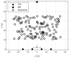
(a) NLoS scenario with $K=4$.

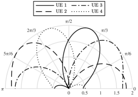
(b) Corresponding covariance shaping vectors.

Figure 6: Multi-UE case: (a) 2D map of the considered NLoS scenario with $K=4$ and variable inter-UE distance $d$; (b) corresponding covariance shaping vectors with $N=2$ obtained with Algorithm 2.

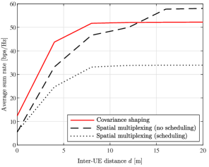
Figure 7: Multi-UE case: average sum rate versus the inter-UE distance $d$ for the NLoS scenario depicted in Fig. 6(a), with $M=128$, ULA at the BS, and $\rho_{\textnormal{\tiny{BS}}}=30$ dBm.

We conclude this section by considering the NLoS scenario in Fig. 8 with $K=8$. Here, the BS is equipped with a UPA and is placed at a height of $20$ m with respect to the UEs and the scatterers. Moreover, the UEs are separated into two groups with inter-group distance $D=20$ m and the inter-UE distance is $d=2$ m, which results in highly overlapping channel covariance matrices within the same group. In this setting, $P=4$ orthogonal pilots are assigned such that two adjacent UEs always utilize orthogonal pilots and covariance shaping is applied independently to each group. Fig. 9 plots the average sum rate versus the transmit power at the BS $\rho_{\textnormal{\tiny{BS}}}$ for different numbers of BS antennas $M$. Note that $M=64$ corresponds to $M_{x}=M_{y}=8$, whereas $M=128$ corresponds to $M_{x}=16$ and $M_{y}=8$. As in Fig. 7, we also study the case where the UEs in each group are scheduled into two separate subgroups of non-adjacent UEs without pilot contamination among groups (scheduling). The signal subspace separation enforced by covariance shaping during both the uplink pilot-aided channel estimation phase and the downlink data transmission phase becomes even more beneficial when the BS is equipped with a UPA with limited spatial selectivity in the azimuth direction. Again, the scheduling approach is shown to further deteriorate the performance of spatial multiplexing due to the pre-log factor of $1/2$ in the sum rate despite avoiding the pilot contamination within the same group.

VI Conclusions

In this paper, we introduce the novel concept of MIMO covariance shaping as a means to achieve statistical orthogonality among interfering UEs. It consists in preemptively applying a statistical beamforming at each UE during both the uplink pilot-aided channel estimation phase and the downlink data transmission phase, aiming at enforcing a separation of the signal subspaces of the UEs that would be otherwise highly overlapping. The proposed MIMO covariance shaping framework exploits the realistic non-Kronecker structure of massive MIMO channels, which allows to suitably alter the channel statistics perceived at the BS by designing the transceiver at the UE-side. To compute the covariance shaping strategies, we present a low-complexity block coordinate descent algorithm that minimizes the inter-UE interference (as a metric to measure the spatial correlation), which is proved to converge to a limit point of the original nonconvex problem or to a stationary point in the two-UE case. We provide numerical results characterizing several scenarios where MIMO covariance shaping outperforms a reference schemes employing the multiple antennas at the UE for spatial multiplexing. Specifically, this occurs when the spatial selectivity of the BS is not sufficient to separate UEs exhibiting high spatial correlation, (e.g., when the BS is equipped with a UPA with limited spatial selectivity in the azimuth direction) and the channel estimation is limited by strong pilot contamination. Future work will consider MIMO covariance shaping in combination with multi-stream transmission and will analyze the trade-off between statistical orthogonality and spatial multiplexing.

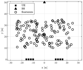
Figure 8: Multi-UE case: (a) 2D map of the considered NLoS scenario with $K=8$, inter-UE distance $d=2$ m, and inter-group distance $D=20$ m.

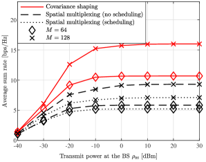
Figure 9: Multi-UE case: average sum rate versus the transmit power at the BS $\rho_{\textnormal{\tiny{BS}}}$ for the NLoS scenario depicted in Fig. 8, with UPA at the BS and for different values of $M$.

Appendix A Derivations of the Effective SINR in (16)

In this Appendix, we derive the expectation terms in (15) to obtain the expression of the effective SINR in (16). First of all, given the multi-UE effective channel matrix $\bar{\mathbf{H}}=[\bar{\mathbf{g}}_{1}^{\mathrm{T}},\ldots,\bar{\mathbf{g}}_{K}^{\mathrm{T}}]^{\mathrm{T}}$, where the effective channels $\{\bar{\mathbf{g}}_{k}\}_{k=1}^{K}$ are independent and $\bar{\mathbf{g}}_{k}\sim\mathcal{C}\mathcal{N}(\mathbf{0},\bar{\mathbf{\Phi}}_{k})$, it is easy to verify that

$$\mathbb{E}[\|\bar{\mathbf{H}}\|_{\mathrm{F}}^{2}] =\sum_{k=1}^{K}\mathrm{tr}(\bar{\mathbf{\Phi}}_{k}).$$ (47)

Furthermore, recalling the definition of $\hat{\bar{\mathbf{g}}}_{k}$ in (9), we have

$$\mathbb{E}[\bar{\mathbf{g}}_{k}\hat{\bar{\mathbf{g}}}_{k}^{\mathrm{H}}]=\mathrm{tr}(\bar{\mathbf{\Phi}}_{k}\mathbf{Q}_{k}^{-1}\bar{\mathbf{\Phi}}_{k}).$$ (48)

We now focus on deriving $\mathbb{V}[\bar{\mathbf{g}}_{k}\hat{\bar{\mathbf{g}}}_{k}^{\mathrm{H}}]$, with $k\in\mathcal{S}_{p}$. We have

$$\mathbb{V}[\bar{\mathbf{g}}_{k}\hat{\bar{\mathbf{g}}}_{k}^{\mathrm{H}}]$$

$$=\mathbb{E}\big{[}|\bar{\mathbf{g}}_{k}\hat{\bar{\mathbf{g}}}_{k}^{\mathrm{H}}|^{2}\big{]}-\big{|}\mathbb{E}[\bar{\mathbf{g}}_{k}\hat{\bar{\mathbf{g}}}_{k}^{\mathrm{H}}]\big{|}^{2}$$ (49)

$$=\mathbb{E}\bigg{[}\bar{\mathbf{g}}_{k}\bar{\mathbf{\Phi}}_{k}\mathbf{Q}_{k}^{-1}\bigg{(}\bar{\mathbf{g}}_{k}^{\mathrm{H}}+\sum_{j\in\mathcal{S}_{p}\setminus\{k\}}\bar{\mathbf{g}}_{j}^{\mathrm{H}}+\frac{1}{\tau\sqrt{\rho_{\textnormal{\tiny{UE}}}}}\mathbf{Z}\mathbf{p}_{p}^{\mathrm{H}}\bigg{)}$$

$$\phantom{=}\ \times\bigg{(}\bar{\mathbf{g}}_{k}+\sum_{j\in\mathcal{S}_{p}\setminus\{k\}}\bar{\mathbf{g}}_{j}+\frac{1}{\tau\sqrt{\rho_{\textnormal{\tiny{UE}}}}}\mathbf{p}_{p}\mathbf{Z}^{\mathrm{H}}\bigg{)}\mathbf{Q}_{k}^{-1}\bar{\mathbf{\Phi}}_{k}\bar{\mathbf{g}}_{k}^{\mathrm{H}}\bigg{]}$$

$$\phantom{=}\ -\mathrm{tr}(\bar{\mathbf{\Phi}}_{k}\mathbf{Q}_{k}^{-1}\bar{\mathbf{\Phi}}_{k})^{2}$$ (50)

$$=\mathbb{E}[\bar{\mathbf{g}}_{k}\bar{\mathbf{\Phi}}_{k}\mathbf{Q}_{k}^{-1}\bar{\mathbf{g}}_{k}^{\mathrm{H}}\bar{\mathbf{g}}_{k}\mathbf{Q}_{k}^{-1}\bar{\mathbf{\Phi}}_{k}\bar{\mathbf{g}}_{k}^{\mathrm{H}}]$$

$$\phantom{=}\ +\sum_{j\in\mathcal{S}_{p}\setminus\{k\}}\mathbb{E}[\bar{\mathbf{g}}_{k}\bar{\mathbf{\Phi}}_{k}\mathbf{Q}_{k}^{-1}\bar{\mathbf{g}}_{j}^{\mathrm{H}}\bar{\mathbf{g}}_{j}\mathbf{Q}_{k}^{-1}\bar{\mathbf{\Phi}}_{k}\bar{\mathbf{g}}_{k}^{\mathrm{H}}]$$

$$\phantom{=}\ +\frac{1}{\tau^{2}\rho_{\textnormal{\tiny{UE}}}}\mathbb{E}[\bar{\mathbf{g}}_{k}\bar{\mathbf{\Phi}}_{k}\mathbf{Q}_{k}^{-1}\mathbf{Z}\mathbf{p}_{p}^{\mathrm{H}}\mathbf{p}_{p}\mathbf{Z}^{\mathrm{H}}\mathbf{Q}_{k}^{-1}\bar{\mathbf{\Phi}}_{k}\bar{\mathbf{g}}_{k}^{\mathrm{H}}]$$

$$\phantom{=}\ -\mathrm{tr}(\bar{\mathbf{\Phi}}_{k}\mathbf{Q}_{k}^{-1}\bar{\mathbf{\Phi}}_{k})^{2}$$ (51)

where in (50) we have used the expression in (48) and where (51) follows from the independence between $\bar{\mathbf{g}}_{k}$ and $\bar{\mathbf{g}}_{j}$, $\forall k\neq j$, and between $\bar{\mathbf{g}}_{k}$ and $\mathbf{Z}$. Then, we write $\bar{\mathbf{g}}_{k}^{\mathrm{H}}=\bar{\mathbf{\Phi}}_{k}^{\frac{1}{2}}\mathbf{x}_{k}$, with $\mathbf{x}_{k}\sim\mathcal{C}\mathcal{N}(0,\mathbf{I}_{M})$, and obtain

$$\mathbb{V}[\bar{\mathbf{g}}_{k}\hat{\bar{\mathbf{g}}}_{k}^{\mathrm{H}}]$$

$$=\mathbb{E}\big{[}\mathbf{x}_{k}^{\mathrm{H}}\bar{\mathbf{\Phi}}_{k}^{\frac{1}{2}}\bar{\mathbf{\Phi}}_{k}\mathbf{Q}_{k}^{-1}\bar{\mathbf{\Phi}}_{k}^{\frac{1}{2}}\mathbf{x}_{k}\mathbf{x}_{k}^{\mathrm{H}}\bar{\mathbf{\Phi}}_{k}^{\frac{1}{2}}\mathbf{Q}_{k}^{-1}\bar{\mathbf{\Phi}}_{k}\bar{\mathbf{\Phi}}_{k}^{\frac{1}{2}}\mathbf{x}\big{]}$$

$$\phantom{=}\ +\sum_{j\in\mathcal{S}_{p}\setminus\{k\}}\mathrm{tr}(\bar{\mathbf{\Phi}}_{k}^{2}\mathbf{Q}_{k}^{-1}\bar{\mathbf{\Phi}}_{j}\mathbf{Q}_{k}^{-1}\bar{\mathbf{\Phi}}_{k})$$

$$\phantom{=}\ +\frac{1}{\tau\varrho_{\textnormal{\tiny{UE}}}}\mathrm{tr}(\bar{\mathbf{\Phi}}_{k}^{2}\mathbf{Q}_{k}^{-2}\bar{\mathbf{\Phi}}_{k})-\mathrm{tr}(\bar{\mathbf{\Phi}}_{k}\mathbf{Q}_{k}^{-1}\bar{\mathbf{\Phi}}_{k})^{2}$$ (52)

$$=\mathrm{tr}(\bar{\mathbf{\Phi}}_{k}^{2}\mathbf{Q}_{k}^{-1}\bar{\mathbf{\Phi}}_{k}\mathbf{Q}_{k}^{-1}\bar{\mathbf{\Phi}}_{k})+\mathrm{tr}(\bar{\mathbf{\Phi}}_{k}\mathbf{Q}_{k}^{-1}\bar{\mathbf{\Phi}}_{k})^{2}$$

$$\phantom{=}\ +\sum_{j\in\mathcal{S}_{p}\setminus\{k\}}\mathrm{tr}(\bar{\mathbf{\Phi}}_{k}^{2}\mathbf{Q}_{k}^{-1}\bar{\mathbf{\Phi}}_{j}\mathbf{Q}_{k}^{-1}\bar{\mathbf{\Phi}}_{k})$$

$$\phantom{=}\ +\frac{1}{\tau\varrho_{\textnormal{\tiny{UE}}}}\mathrm{tr}(\bar{\mathbf{\Phi}}_{k}^{2}\mathbf{Q}_{k}^{-2}\bar{\mathbf{\Phi}}_{k})-\mathrm{tr}(\bar{\mathbf{\Phi}}_{k}\mathbf{Q}_{k}^{-1}\bar{\mathbf{\Phi}}_{k})^{2}$$ (53)

$$=\mathrm{tr}\bigg{(}\bar{\mathbf{\Phi}}_{k}^{2}\mathbf{Q}_{k}^{-1}\bigg{(}\bar{\mathbf{\Phi}}_{k}+\sum_{j\in\mathcal{S}_{p}\setminus\{k\}}\bar{\mathbf{\Phi}}_{j}+\frac{1}{\tau\varrho_{\textnormal{\tiny{UE}}}}\mathbf{I}_{M}\bigg{)}\mathbf{Q}_{k}^{-1}\bar{\mathbf{\Phi}}_{k}\bigg{)}$$ (54)

$$=\mathrm{tr}(\bar{\mathbf{\Phi}}_{k}^{2}\mathbf{Q}_{k}^{-1}\bar{\mathbf{\Phi}}_{k})$$ (55)

where (52) is obtained by substituting $\mathbb{E}[\mathbf{Z}\mathbf{p}_{p}^{\mathrm{H}}\mathbf{p}_{p}\mathbf{Z}^{\mathrm{H}}]=\tau\sigma_{\textnormal{\tiny{BS}}}^{2}\mathbf{I}_{M}$, in (53) we have exploited the fact that $\mathbb{E}[\mathbf{x}_{k}\mathbf{x}_{k}^{\mathrm{H}}\mathbf{A}\mathbf{x}_{k}\mathbf{x}_{k}^{\mathrm{H}}]=\mathbf{A}+\mathrm{tr}(\mathbf{A})\mathbf{I}_{M}$ for a given Hermitian matrix $\mathbf{A}\in\mbox{$\mathbb{C}$}^{M\times M}$ [13, App. A.2], and in (55) we have used the definition of $\mathbf{Q}_{k}$ provided in Section III-A. Finally, we focus on deriving $\mathbb{E}\big{[}|\bar{\mathbf{g}}_{k}\hat{\bar{\mathbf{g}}}_{j}^{\mathrm{H}}|^{2}\big{]}$, with $k\in\mathcal{S}_{p}$ and with $j\in\mathcal{S}_{q}$. Following similar steps as above, we have

$$\mathbb{E}\big{[}|\bar{\mathbf{g}}_{k}\hat{\bar{\mathbf{g}}}_{j}^{\mathrm{H}}|^{2}\big{]}$$

$$=\mathbb{E}\bigg{[}\bar{\mathbf{g}}_{k}\bar{\mathbf{\Phi}}_{j}\mathbf{Q}_{j}^{-1}\bigg{(}\bar{\mathbf{g}}_{j}^{\mathrm{H}}+\sum_{l\in\mathcal{S}_{q}\setminus\{j\}}\bar{\mathbf{g}}_{l}^{\mathrm{H}}+\frac{1}{\tau\sqrt{\rho_{\textnormal{\tiny{UE}}}}}\mathbf{Z}\mathbf{p}_{q}^{\mathrm{H}}\bigg{)}$$

$$\phantom{=}\ \times\bigg{(}\bar{\mathbf{g}}_{j}+\sum_{l\in\mathcal{S}_{q}\setminus\{j\}}\bar{\mathbf{g}}_{l}+\frac{1}{\tau\sqrt{\rho_{\textnormal{\tiny{UE}}}}}\mathbf{p}_{q}\mathbf{Z}^{\mathrm{H}}\bigg{)}\mathbf{Q}_{j}^{-1}\bar{\mathbf{\Phi}}_{j}\bar{\mathbf{g}}_{k}^{\mathrm{H}}\bigg{]}$$ (56)

$$=\mathbb{E}[\bar{\mathbf{g}}_{k}\bar{\mathbf{\Phi}}_{j}\mathbf{Q}_{j}^{-1}\bar{\mathbf{g}}_{j}^{\mathrm{H}}\bar{\mathbf{g}}_{j}\mathbf{Q}_{j}^{-1}\bar{\mathbf{\Phi}}_{j}\bar{\mathbf{g}}_{k}^{\mathrm{H}}]$$

$$\phantom{=}\ +\sum_{l\in\mathcal{S}_{q}\setminus\{j\}}\mathbb{E}[\bar{\mathbf{g}}_{k}\bar{\mathbf{\Phi}}_{j}\mathbf{Q}_{j}^{-1}\bar{\mathbf{g}}_{l}^{\mathrm{H}}\bar{\mathbf{g}}_{l}\mathbf{Q}_{j}^{-1}\bar{\mathbf{\Phi}}_{j}\bar{\mathbf{g}}_{k}^{\mathrm{H}}]$$

$$\phantom{=}\ +\frac{1}{\tau^{2}\rho_{\textnormal{\tiny{UE}}}}\mathbb{E}[\bar{\mathbf{g}}_{k}\bar{\mathbf{\Phi}}_{k}\mathbf{Q}_{k}^{-1}\mathbf{Z}\mathbf{p}_{q}^{\mathrm{H}}\mathbf{p}_{q}\mathbf{Z}^{\mathrm{H}}\mathbf{Q}_{k}^{-1}\bar{\mathbf{\Phi}}_{k}\bar{\mathbf{g}}_{k}^{\mathrm{H}}]$$ (57)

$$=\mathrm{tr}(\bar{\mathbf{\Phi}}_{k}\bar{\mathbf{\Phi}}_{j}\mathbf{Q}_{j}^{-1}\bar{\mathbf{\Phi}}_{j}\mathbf{Q}_{j}^{-1}\bar{\mathbf{\Phi}}_{j})$$

$$\phantom{=}\ +\sum_{l\in\mathcal{S}_{q}\setminus\{j\}}\mathrm{tr}(\bar{\mathbf{\Phi}}_{k}\bar{\mathbf{\Phi}}_{j}\mathbf{Q}_{j}^{-1}\bar{\mathbf{\Phi}}_{l}\mathbf{Q}_{j}^{-1}\bar{\mathbf{\Phi}}_{j})$$

$$\phantom{=}\ +\mathbbm{1}_{q=p}\mathrm{tr}(\bar{\mathbf{\Phi}}_{k}\mathbf{Q}_{j}^{-1}\bar{\mathbf{\Phi}}_{j})^{2}+\frac{1}{\tau\varrho_{\textnormal{\tiny{UE}}}}\mathrm{tr}(\bar{\mathbf{\Phi}}_{k}\bar{\mathbf{\Phi}}_{j}\mathbf{Q}_{j}^{-2}\bar{\mathbf{\Phi}}_{j})$$ (58)

$$=\mathrm{tr}\bigg{(}\bar{\mathbf{\Phi}}_{k}\bar{\mathbf{\Phi}}_{j}\mathbf{Q}_{j}^{-1}\bigg{(}\bar{\mathbf{\Phi}}_{j}+\sum_{l\in\mathcal{S}_{q}\setminus\{j\}}\bar{\mathbf{\Phi}}_{l}+\frac{1}{\tau\varrho_{\textnormal{\tiny{UE}}}}\mathbf{I}_{M}\bigg{)}\mathbf{Q}_{j}^{-1}\bar{\mathbf{\Phi}}_{j}\bigg{)}$$

$$\phantom{=}\ +\mathbbm{1}_{q=p}\mathrm{tr}(\bar{\mathbf{\Phi}}_{k}\mathbf{Q}_{j}^{-1}\bar{\mathbf{\Phi}}_{j})^{2}$$ (59)

$$=\mathrm{tr}(\bar{\mathbf{\Phi}}_{k}\bar{\mathbf{\Phi}}_{j}\mathbf{Q}_{j}^{-1}\bar{\mathbf{\Phi}}_{j})+\mathbbm{1}_{q=p}\mathrm{tr}(\bar{\mathbf{\Phi}}_{k}\mathbf{Q}_{j}^{-1}\bar{\mathbf{\Phi}}_{j})^{2}.$$ (60)

Note that the second term in (60) is active only if UEs $k$ and $j$ are assigned the same pilot.

References

• [1] P. Mursia, I. Atzeni, D. Gesbert, and L. Cottatellucci, “Covariance shaping for massive MIMO systems,” in Proc. IEEE Global Commun. Conf. (GLOBECOM), Abu Dhabi, UAE, Dec. 2018.
• [2] ——, “On the performance of covariance shaping in massive MIMO systems,” in Proc. IEEE Int. Workshop Computer-Aided Modeling and Design of Commun. Links and Netw. (CAMAD), Barcelona, Spain, Sep. 2018.
• [3] F. Boccardi, R. W. Heath, A. Lozano, T. L. Marzetta, and P. Popovski, “Five disruptive technology directions for 5G,” IEEE Commun. Mag., vol. 52, no. 2, pp. 74–80, Feb. 2014.
• [4] E. Larsson, O. Edfors, F. Tufvesson, and T. L. Marzetta, “Massive MIMO for next generation wireless systems,” IEEE Commun. Mag., vol. 52, no. 2, pp. 186–195, Feb. 2014.
• [5] J. G. Andrews, S. Buzzi, W. Choi, S. V. Hanly, A. Lozano, A. C. K. Soong, and J. C. Zhang, “What will 5G be?” IEEE J. Sel. Areas Commun., vol. 32, no. 6, pp. 1065–1082, Jun. 2014.
• [6] N. Rajatheva, I. Atzeni, E. Björnson et al., “White paper on broadband connectivity in 6G,” Jun. 2020. [Online]. Available: http://jultika.oulu.fi/files/isbn9789526226798.pdf
• [7] J. Zhang, E. Björnson, M. Matthaiou, D. Wing, K. Ng, H. Yang, and D. J. Love, “Prospective multiple antenna technologies for beyond 5G,” IEEE J. Sel. Areas Commun., vol. 38, no. 8, pp. 1637–1660, Aug. 2020.
• [8] X. Chen, D. W. K. Ng, W. Yu, E. G. Larsson, N. Al-Dhahir, and R. Schober, “Massive access for 5G and beyond,” IEEE J. Sel. Areas Commun., vol. 39, no. 3, pp. 615–637, Mar. 2021.
• [9] H. Q. Ngo, A. Ashikhmin, H. Yang, E. G. Larsson, and T. L. Marzetta, “Cell-free massive MIMO versus small cells,” IEEE Trans. Wireless Commun., vol. 16, no. 3, pp. 1834–1850, Mar. 2017.
• [10] I. Atzeni, B. Gouda, and A. Tölli, “Distributed precoding design via over-the-air signaling for cell-free massive MIMO,” IEEE Trans. Wireless Commun., vol. 20, no. 2, pp. 1201–1216, Feb. 2021.
• [11] E. Björnson, J. Hoydis, and L. Sanguinetti, “Massive MIMO has unlimited capacity,” IEEE Trans. Wireless Commun., vol. 17, no. 1, pp. 574–590, Jan. 2018.
• [12] J. Jose, A. Ashikhmin, T. L. Marzetta, and S. Vishwanath, “Pilot contamination and precoding in multi-cell TDD systems,” IEEE Trans. Wireless Commun., vol. 10, no. 8, pp. 2640–2651, Aug. 2011.
• [13] T. L. Marzetta, E. G. Larsson, and H. Yang, Fundamentals of Massive MIMO.   Cambridge University Press, 2016.
• [14] J. Nam, J. Y. Ahn, A. Adhikary, and G. Caire, “Joint spatial division and multiplexing: Realizing massive MIMO gains with limited channel state information,” in Proc. Conf. on Inf. Sci. and Sys. (CISS), Princeton, USA, Mar. 2012.
• [15] A. Adhikary, J. Nam, J. Y. Ahn, and G. Caire, “Joint spatial division and multiplexing—The large-scale array regime,” IEEE Trans. Inf. Theory, vol. 59, no. 10, pp. 6441–6463, Jun. 2013.
• [16] J. Nam, A. Adhikary, J. Y. Ahn, and G. Caire, “Joint spatial division and multiplexing: Opportunistic beamforming, user grouping and simplified downlink scheduling,” IEEE J. Sel. Topics Signal Process., vol. 8, no. 5, pp. 876–890, Oct. 2014.
• [17] H. Yin, D. Gesbert, M. Filippou, and Y. Liu, “A coordinated approach to channel estimation in large-scale multiple-antenna systems,” IEEE J. Sel. Areas Commun., vol. 31, no. 2, pp. 264–273, Feb. 2013.
• [18] H. Yin, D. Gesbert, and L. Cottatellucci, “Dealing with interference in distributed large-scale MIMO systems: A statistical approach,” IEEE J. Sel. Topics Signal Process., vol. 8, no. 5, pp. 942–953, Oct. 2014.
• [19] X. Zhang, D. P. Palomar, and B. Ottersten, “Statistically robust design of linear MIMO transceivers,” IEEE Trans. Signal Process., vol. 56, no. 8, pp. 3678–3689, Aug. 2008.
• [20] M. Dai and B. Clerckx, “Transmit beamforming for MISO broadcast channels with statistical and delayed CSIT,” IEEE Trans. Commun., vol. 63, no. 4, pp. 1202–1215, Jan. 2015.
• [21] A. Liu and V. Lau, “Hierarchical interference mitigation for massive MIMO cellular networks,” IEEE Trans. Signal Process., vol. 62, no. 18, pp. 4786–4797, Sep. 2014.
• [22] A. Padmanabhan, A. Tölli, and I. Atzeni, “Distributed two-stage multi-cell precoding,” in Proc. IEEE Int. Workshop Signal Process. Adv. in Wireless Commun. (SPAWC), Cannes, France, Jul. 2019.
• [23] L. You, X. Gao, X. Xia, N. Ma, and Y. Peng, “Pilot reuse for massive MIMO transmission over spatially correlated Rayleigh fading channels,” IEEE Trans. Wireless Commun., vol. 14, no. 6, pp. 3352–3366, Jun. 2015.
• [24] N. N. Moghadam, H. Shokri-Ghadikolaei, G. Fodor, M. Bengtsson, and C. Fischione, “Pilot precoding and combining in multiuser MIMO networks,” IEEE J. Sel. Areas Commun., vol. 35, no. 7, pp. 1632–1648, Jul. 2017.
• [25] H. Yin, L. Cottatellucci, D. Gesbert, R. R. Müller, and G. He, “Robust pilot decontamination based on joint angle and power domain discrimination,” IEEE Trans. Signal Process., vol. 64, no. 11, pp. 2990–3003, Feb. 2016.
• [26] R. Müller, L. Cottatellucci, and M. Vehkaperä, “Blind pilot decontamination,” IEEE J. Sel. Topics Signal Process., vol. 8, no. 5, pp. 773–786, Oct. 2014.
• [27] V. Raghavan, J. H. Kotecha, and A. M. Sayeed, “Why does the Kronecker model result in misleading capacity estimates?” IEEE Trans. Inf. Theory, vol. 56, no. 10, pp. 4843–4864, Oct. 2010.
• [28] W. Weichselberger, M. Herdin, H. Özcelik, and E. Bonek, “A stochastic MIMO channel model with joint correlation of both link ends,” IEEE Trans. Wireless Commun., vol. 5, no. 1, pp. 90–100, Jan. 2006.
• [29] Y. C. Eldar and A. V. Oppenheim, “Covariance shaping least-squares estimation,” IEEE Trans. Signal Process., vol. 51, no. 3, pp. 686–697, Mar. 2003.
• [30] A. K. Hassan, M. Moinuddin, U. M. Al-Saggaf, O. Aldayel, T. N. Davidson, and T. Y. Al-Naffouri, “Performance analysis and joint statistical beamformer design for multi-user MIMO systems,” IEEE Commun. Lett., vol. 24, no. 10, pp. 2152–2156, Oct. 2020.
• [31] A. Paulraj, R. Nabar, and D. Gore, Introduction to Space-Time Wireless Communications.   Cambridge University Press, 2006.
• [32] E. Björnson, J. Hoydis, and L. Sanguinetti, “Massive MIMO networks: Spectral, energy, and hardware efficiency,” Foundations and Trends® Signal Process., vol. 11, no. 3–4, pp. 154–655, Nov. 2017.
• [33] E. Dahlman, S. Parkvall, and J. Skold, 5G NR: The Next Generation Wireless Access Technology.   Academic Press, 2018.
• [34] L. Grippo and M. Sciandrone, “On the convergence of the block nonlinear Gauss-Seidel method under convex constraints,” Operation Res. Lett., vol. 26, no. 3, pp. 127–136, Apr. 2000.
• [35] G. Scutari, F. Facchinei, P. Song, D. P. Palomar, and J.-S. Pang, “Decomposition by partial linearization: Parallel optimization of multi-agent systems,” IEEE Trans. Signal Process., vol. 62, no. 3, pp. 641–656, Feb. 2014.
• [36] Q. H. Spencer, A. L. Swindlehurst, and M. Haardt, “Zero-forcing methods for downlink spatial multiplexing in multiuser MIMO channels,” IEEE Trans. Signal Process., vol. 52, no. 2, pp. 461–471, Feb. 2004.
• [37] S. Christensen, R. Agarwal, E. Carvalho, and J. Cioffi, “Weighted sum-rate maximization using weighted MMSE for MIMO-BC beamforming design,” IEEE Trans. Wireless Commun., vol. 7, no. 12, pp. 4792–4799, Dec. 2008.
• [38] A. M. Sayeed, “Deconstructing multiantenna fading channels,” IEEE Trans. Signal Process., vol. 50, no. 10, pp. 2563–2579, Oct. 2002.