A stochastic metapopulation state-space approach to modeling and estimating Covid-19 spread

Abstract

Mathematical models are widely recognized as an important tool for analyzing and understanding the dynamics of infectious disease outbreaks, predict their future trends, and evaluate public health intervention measures for disease control and elimination. We propose a novel stochastic metapopulation state-space model for COVID-19 transmission, based on a discrete-time spatio-temporal susceptible/exposed/infected/recovered/deceased (SEIRD) model. The proposed framework allows the hidden SEIRD states and unknown transmission parameters to be estimated from noisy, incomplete time series of reported epidemiological data, by application of unscented Kalman filtering (UKF), maximum-likelihood adaptive filtering, and metaheuristic optimization. Experiments using both synthetic data and real data from the Fall 2020 Covid-19 wave in the state of Texas demonstrate the effectiveness of the proposed model.

Keywords epidemic model  $\cdot$ SEIRD model  $\cdot$ nonlinear stochastic model  $\cdot$ unscented Kalman filter  $\cdot$ maximum likelihood  $\cdot$ adaptive filtering  $\cdot$ parameter estimation

1 Introduction

Infectious disease outbreaks remain a major threat to global health. This is especially the case for highly pathogenic and transmissible diseases with pandemic potential. These global threats were recently exemplified by the 2009 swine flu outbreak and the ongoing COVID-19 pandemic caused by the novel Severe Acute Respiratory Syndrome coronavirus 2 (SARS-CoV-2). To effectively mitigate and control the spread of an epidemic, it is paramount for public health decision-making to be informed by an accurate understanding of the dynamics of disease transmission and the potential impact of intervention measures. To this end, epidemic models have become an important tool to help better understand epidemic dynamics, predict its future trends, evaluate the effectiveness of intervention measures, such as lock-down or vaccination, and ultimately control the epidemic.

Mathematical epidemiology models can be broadly divided into two main types: compartmental models and agent-based models. An agent-based model is a very detailed stochastic model where the agent represent single individuals within a population Degli Atti et al. (2008); Perez and Dragicevic (2009); Hunter et al. (2018); Chang et al. (2020); Chao et al. (2020); Koo et al. (2020); Kretzschmar et al. (2020); Kerr et al. (2020). Such models are generally complex and computationally expensive. In compartmental models, the population is subdivided into epidemiological compartments with each compartmental generally representing a health or disease progression stage Balcan et al. (2010); Dukic et al. (2012); Osthus et al. (2017); Sebastian and Victor (2017); Keeling et al. (2020); Sameni (2020); Godio et al. (2020); Kobayashi et al. (2020). Thus compartmental models are computationally simple, scalable, and capable of describing the dynamics of the number of people in each compartment throughout the course of an epidemic. In this work, we propose a nonlinear state-space compartmental model.

Compartmental model date back to the early twentieth century, most notably to the work by Kermack and McKendrick (1927), whose susceptible/infected/recovered (SIR) model was used for modeling the plague (London 1665-1666, Bombay 1906) and cholera (London 1865) epidemics Dukic et al. (2012). More specifically, it is a weighted directed graph representation of a dynamic system. The susceptible refers to those healthy people who are susceptible to the disease and may get infected; the infected refers to those under infection; the recovered refers to those who recovered from infection and will be temporarily or permanently immune to the disease. However, there are several drawbacks in the original SIR model:

• It is a deterministic model, meaning the model always performs the same for a given initial condition, which cannot explain the unknowable randomness in the observations Sebastian and Victor (2017); Hooker et al. (2011); Kobayashi et al. (2020);

• It is only a temporal model, which does not consider the spread in geographical regions, e.g. human interaction induced by modern transportation Zhong et al. (2009);

• It assumes that all the parameters are known, which is not realistic. Parameter estimation from noisy observations is needed for better understanding and forecasting epidemics Hooker et al. (2011).

Many variants SIR models have been proposed to address some of these issues, but accurate state and parameter estimation from partial and noisy observations remains an open problem. To‘ handle this issue, our proposed framework embeds the classical compartmental model within a nonlinear state-space model. The state model is a spatial-temporal stochastic dynamic model that allows hidden states in a given location to change over time and the disease dynamics in one location to affect neighbouring locations through human movements between locations. The proposed framework consists of a multinomial state model based on a variant of the SIR model — the SEIRD model Rapolu et al. (2020); Piccolomiini and Zama (2020); Korolev (2021) — and an observation model to allow the assimilation of publicly available data, including daily testing rate, daily test positivity rate, specificity and sensitivity of the tests. In addition, the model considers the differential testing rate between symptomatic patients and asymptomatic and healthy individuals. The proposed framework is employed to estimate i) the hidden epidemic state vector $X^{t}=(S^{t},E^{t},I^{t},R^{t},D^{t})$ and ii) epidemiological parameters, such as infection rate and the average infectious period, using noisy incomplete time series epidemic data. Accurate estimation of the true epidemic state and parameters is paramount for designing and evaluating the effectiveness of control strategies.

2 Mathematical model

2.1 Classical SEIRD model

The SEIRD model predicts the time evolution of epidemic. It models the dynamic interaction of people between five different compartments, namely, the susceptible (S), the exposed (E), the infected (I), the recovered (R) and the deceased (D). The classic continuous-time SEIRD model can be described by the following equations:

$$\frac{dS(t)}{dt} \,=\,-\lambda_{S}S(t)I(t)$$ (1)

$$\frac{dE(t)}{dt} \,=\,\lambda_{S}S(t)I(t)-\lambda_{E}E(t)$$

$$\frac{dI(t)}{dt} \,=\,\lambda_{E}E(t)-(\lambda_{R}+\lambda_{D})I(t)$$

$$\frac{dR(t)}{dt} \,=\,\lambda_{R}I(t)$$

$$\frac{dD(t)}{dt} \,=\,\lambda_{D}I(t)$$

with $S(t)+E(t)+I(t)+R(t)+D(t)\,=\,1$, where $S(t)$, $E(t)$, $I(t)$, $R(t)$, $D(t)$ are the fraction of the population (the size of which is assumed to be constant over the time interval of interest) at time $t$ that, respectively, $S$ is not yet infected with the disease; $E$ has been exposed to the virus but does not show symptoms yet; $I$ is infective after the virus incubation period; $R$ has been infected and then recovered; and $D$ is deceased due to the epidemic.

The model is governed by the following parameters:

• $\lambda_{S}$ is the infection rate, which is the probability that an individual moves from the S to the E compartment. The nonlinear term $\lambda_{S}I(t)S(t)$ models the infection speed, which depends not only on the infection rate, but also on the fraction of susceptible and infected people at time $t$;

• $\lambda_{E}$ is the probability that an individual moves from the E to the I compartment. It can be understood as the inverse of the average incubation time;

• $\lambda_{R}$ is the recovery rate, which is the probability than an individual moves from the I to the R compartment. It can be understodd as the inverse of the average recovery time;

• $\lambda_{D}$ is the mortality rate, which is the probability than an individual moves from the I to the D compartment.

2.2 Covid-19 epidemic metapopulation state-space model

Given the complexity and reality of epidemics, many different implementations of the classical SEIRD model have been proposed Loli Piccolomini and Zama (2020); Korolev (2021); Tiwari et al. (2020); Rapolu et al. (2020). Two clear drawbacks of the classical SEIRD model is the inability to model variation over a geographic area, and the fact that that the SEIRD values are assumed to be directly observable. In this paper, we address these drawbacks by means of a novel nonlinear metapolulation state-space framework, where the state process provides a spatial-temporal discrete-time stochastic model of the evolution of the number of individuals in the SEIRD compartments over several geographical regions, while the observation process models noisy time series of reported epidemiological data, considering the accuracy of tests and different testing rates for symptomatic and asymptomatic people.

2.2.1 State model

Consider a discrete-time state process $\{{\mathbf{X}}_{i}^{t};i=1,\dots,G;t=0,1,\dots\}$, where ${\mathbf{X}}_{i}^{t}=(S_{i}^{t},E_{i}^{t},I_{i}^{t},R_{i}^{t},D_{i}^{t})$ is a state vector, containing the number of individuals in the SEIRD compartments in geographical area $i$ at time $t$, where the unit of time is typically day or week. At time $t$, the total number of individuals in region $i$ is $N_{i}=S_{i}^{t}+E_{i}^{t}+I_{i}^{t}+R_{i}^{t}+D_{i}^{t}$. We assume that this number stays constant over the time interval of interest (e.g., no significant amounts of migration is assumed to occur during the time interval of interest; plus , births and non-specific deaths are assumed to approximately balance out). This results in a good approximation provided that the interval of time in consideration consists of weeks or a few months, especially in the case of a full-blown outbreak when, the impact of migration is negligible.

Before proceeding, we recall the definition of the binomial and multinomial probability distributions. A random variable $Z$ has a binomial distribution with parameters $n\geq 1$ and $0<p<1$, denoted by $Z\sim{\rm Binomial}(n,p)$, if

$$P(Z=k)\,=\,\frac{n!}{k!(n-k)!}\,p^{k}(1-p)^{n-k},\quad k=0,\ldots,n\,.$$ (2)

where $n!=n\times n-1\times\cdots 1$, with $0!=1$. Variable $Z$ is the number of $k$ occurrences of an outcome among $n$ identical independent trials that can result in the outcome with probability $p$. The expected value and variance of this variable are $E[Z]=np$ and ${\rm Var}(Z)=np(1-p)$, respectively. More generally, we define a random vector $(Z_{1},\ldots,Z_{M})$ to have a multinomial distribution with parameters $n\geq 1$ and $p_{1},\ldots,p_{M}\geq 0$ such that $\sum p_{i}\leq 1$, denoted by $(Z_{1},\ldots,Z_{M})\sim{\rm Multinomial}(n,p_{1},\ldots,p_{M})$, if

$$P(Z_{1}=k_{1},\ldots,Z_{M}=k_{M})\,=\,\frac{n!}{k_{1}!\cdots k_{M}!(n\!-\!\Sigma k_{i})!}\,p_{1}^{k_{1}}\cdots p_{M}^{k_{M}}(1\!-\!\Sigma p_{i})^{n-\Sigma k_{i}},\quad k_{1},\ldots,k_{M}\geq 0,\>\Sigma k_{i}\leq n\,.$$ (3)

Variables $Z_{1},\ldots,Z_{M}$ are the number of occurrences of each of $M$ outcomes over $n$ identical independent trials that can result in outcome $m$ with probability $p_{m}$. It is clear that $Z_{m}\sim{\rm Binomial}(n,p_{m})$, for $m=1,\ldots,M$ (thus $E[Z_{m}]=np_{m}$ and ${\rm Var}(Z_{m})=np_{m}(1-p_{m})$). In addition, the case $M=1$ results in the binomial distribution.

In our model, the state vector ${\mathbf{X}}_{i}^{t}=(S_{i}^{t},E_{i}^{t},I_{i}^{t},R_{i}^{t},D_{i}^{t})$ is assumed to evolve according to the following nonlinear stochastic model:

$$S_{i}^{t+1} =\,S_{i}^{t}\,-\,\Sigma_{j}\,N_{S_{i,j}}^{t}$$ (4)

$$E_{i}^{t+1} =\,E_{i}^{t}\,+\,\Sigma_{j}\,N_{S_{i,j}}^{t}\,-\,N_{E_{i}}^{t}$$

$$I_{i}^{t+1} =\,I_{i}^{t}\,+\,N_{E_{i}}^{t}\,-\,N_{R_{i}}^{t}\,-\,N_{D_{i}}^{t}$$

$$R_{i}^{t+1} =\,R_{i}^{t}\,+\,N_{R_{i}}^{t}$$

$$D_{i}^{t+1} =\,D_{i}^{t}\,+\,N_{D_{i}}^{t}$$

for $t=0,1,\ldots$, where $N^{t}_{S_{i,j}}$ is the number of susceptible individuals at time $t$ in region $i$ who will become exposed at time $t+1$ due to contact with an infective individual from region $j$, $N^{t}_{E_{i}}$ is the number of exposed people at time $t$ in region $i$ who will become infective at time $t+1$, while $N^{t}_{R_{i}}$ and $N^{t}_{D_{i}}$ are the numbers of infected people at time $t$ in region $i$ who will become recovered or deceased at time $t+1$, respectively.

We assume that each susceptible individual in region $i$ becomes exposed due to contact with an infective individual from region $j$ at time $t$ independently with a probability $\lambda_{S}c_{ij}I_{j}^{t}/N_{j}$ (these parameters are explained below). Therefore, the distribution of the numbers of new infections over the regions is multinomial:

$$(N_{S_{i,1}}^{t},\ldots,N_{S_{i,G}}^{t})\,\sim\,{\rm Multinomial}\left(S_{i}^{t},\lambda_{S}\frac{c_{i1}I_{1}^{t}}{N_{1}},\dots,\lambda_{S}\frac{c_{iG}I_{G}^{t}}{N_{G}}\right).$$ (5)

The infection rate $\lambda_{S}>0$ is disease-specific, but also affected by public policies, such as mask wearing and social distancing. We assume that these factors are constant over the geographical area (e.g., a single political unit, such as a state or country) and time interval in the study, so that $\lambda_{S}$ is the same for all regions. If $i=j$, then the contact is internal to region $i$, and $c_{ii}=1$. If $i\neq j$, then $0\leq c_{ij}\leq 1$ models the relative amount of transient interchange of individuals between regions $i$ and $j$, due to commuting, tourism, and so on. If regions $i$ and $j$ are far apart, or one of them is not economically important, then $c_{ij}$ is close to zero. Note that $c_{ij}=c_{ji}$. The specific values of $c_{ij}$ are selected in our study based on the gravity model Zipf (1946); Truscott and Ferguson (2012); Chen et al. (2021); Finally, the ratio $I_{j}^{t}/N_{j}$ indicates that if there are more infective individuals in region $j$, they will spread the disease with higher probability. Note that the expected value of the (normalized) $j$-th flux is $E[N_{S_{i,j}}^{t}/N_{i}]=\lambda_{S}c_{ij}(S_{i}^{t}/N_{i})(I_{j}^{t}/N_{j})$. This may be contrasted to the flux $\lambda_{S}S(t)I(t)$ in the classical case.

In our model, an exposed individual in region $i$ becomes infective at time $t$, independently of the other regions, with probability $\lambda_{E}$. Hence,

$$N_{E_{i}}^{t}\,\sim\,{\rm Binomial}(E_{i}^{t},\lambda_{E})\,.$$ (6)

The expected number of exposed individuals who become infective at time $t$ is thus $E[N_{E_{i}}^{t}]=\lambda_{E}E_{i}^{t}$. Note also that the distribution of the total time until an exposed individual becomes infective is geometric with parameter $\lambda_{E}$, so that the expected number of time units until an exposed individual becomes infective is $\lambda_{E}^{-1}$.

Finally, each infective individual in region $i$ becomes recovered or deceased at time $t$, independently of the other regions, with probabilities $\lambda_{R}$ and $\lambda_{D}$, respectively. Hence,

$$(N_{R_{i}}^{t},N_{D_{i}}^{t})\,\sim\,{\rm Multinomial}(I_{i}^{t},\lambda_{R},\lambda_{D})\,.$$ (7)

The expected numbers of infective individuals who become recovered or deceased at time $t$ are $E[N_{R_{i}}^{t}]=\lambda_{R}I_{i}^{t}$ and $E[N_{D_{i}}^{t}]=\lambda_{D}I_{i}^{t}$, respectively. The expected numbers of time units until an infective individual becomes recovered or deceased are $\lambda_{R}^{-1}$ and $\lambda_{D}^{-1}$, respectively.

2.2.2 Observation model

The observation model is a major contribution of this work. We model reported epidemiological data, namely confirmed new cases and cumulative recorded deaths, as noisy observations on the true state of the pandemic, as defined in the previous section. The proposed observation model addresses the uncertainty introduced by imperfect testing and the imbalance in testing of symptomatic and asymptomatic individuals (the former cohort is tested more Allen et al. (2020)).

We model the reported data as a time series $\{{\mathbf{Y}}_{i}^{t};i=1,\dots,G;t=0,1,\dots\}$ where ${\mathbf{Y}}_{i}^{t}=(P_{i}^{t},Q_{i}^{t})$ contains the numbers $P_{i}^{t}$ and $Q_{i}^{t}$ of new confirmed cases and deaths, respectively, in geographical area $i$ at time $t$. The number of reported new cases contain both false and true positives,

$$P_{i}^{t}\,=\,N_{TP_{i}}^{t}\,+\,N_{FP_{i}}^{t},$$ (8)

for $t=0,1,,\ldots$, where $N_{TP_{i}}^{t}$ and $N_{FP_{i}}^{t}$ are the number of false and true testing positives, respectively. Let $\alpha$ and $\beta$ be the false positive and true positive rates, respectively, of the Covid-19 test under consideration (multiple tests of different accuracy can be introduced by splitting the populations according to the test received). True positives come from the exposed and infective populations. In addition, a percentage of the infective population is asymptomatic; we assume that those are tested at a smaller rate than the symptomatic ones. Accordingly, we split the number of new true positives at time $t$ as the sum of the number of positive-tested symptomatic infective people and the number of positive-tested asymptomatic infective and exposed individuals:

$$N_{TP_{i}}^{t}\,\sim\,{\rm Binomial}(\varepsilon^{t}_{2}(1-\varepsilon^{t}_{4})I_{i}^{t},\,\beta)\,+\,{\rm Binomial}(\varepsilon^{t}_{1}(\varepsilon^{t}_{4}I_{i}^{t}+E_{i}^{t}),\,\beta)\,,$$ (9)

where $\varepsilon^{t}_{1}$ and $\varepsilon^{t}_{2}$ are the testing rates of asymptomatic and symptomatic individuals at time $t$, respectively, while $\varepsilon^{t}_{4}$ is the percentage of infective individuals who are asymptomatic at time $t$. These parameters are assumed to be the same over all regions. As shown later, these parameters can be calculated from the overall testing and positivity rates, which are available from public records.

Similarly, the false positives come from the susceptible and recovered populations, and here we have to distinguish between symptomatic individuals (who are not infected by Covid-19 but instead by other similar viruses, such as Influenza) and asymptomatic individuals:

$$N_{FP_{i}}^{t}\,\sim\,{\rm Binomial}(\varepsilon^{t}_{1}(1-\varepsilon^{t}_{3})(S_{i}^{t}+R_{i}^{t}),\,\alpha)\,+\,{\rm Binomial}(\varepsilon^{t}_{2}\varepsilon^{t}_{3}(S_{i}^{t}+R_{i}^{t}),\,\alpha)\,,$$ (10)

where $\varepsilon^{t}_{3}$ is the percentage of non-specific symptomatic individuals at time $t$.

Finally, we assume that the reported cumulative recorded deaths in each region is a fraction of the true number $D_{i}^{t}$, according to

$$Q_{i}^{t}\,\sim\,{\rm Binomial}(D_{i}^{t},\,\beta)\,.$$ (11)

Even though there might be a number of non-Covid-19 deaths falsely reported as Covid-19, we are assuming that this number is small and can be ignored. Notice that (11) implies that Covid-19 deaths are underreported, which is widely assumed to be the case.

Let $R_{T}^{t}$ be the testing rate, i.e., the percentage of the population that is tested at time $t$, and let $R_{P}^{t}$ the positivity rate at time $t$. Both these parameters are reported by health authorities. Next, we show how the parameters $\varepsilon^{t}_{1}$, $\varepsilon^{t}_{2}$, $\varepsilon^{t}_{3}$, and $\varepsilon^{t}_{4}$ can be calculated from $R_{T}^{t}$ and $R_{P}^{t}$

The test positivity rate ($R_{P}^{t}$) is the percentage of positive tests $P^{t}$ over the total number of tests $N_{T}^{t}$ in a given region; it can be written as

$$R_{P}^{t}\,=\,\frac{P^{t}}{N_{T}^{t}}\,=\,\frac{\varepsilon^{t}_{1}A\alpha+\varepsilon^{t}_{2}B\alpha+\varepsilon^{t}_{2}C\beta+\varepsilon^{t}_{1}D\beta}{\varepsilon^{t}_{1}A+\varepsilon^{t}_{2}B+\varepsilon^{t}_{2}C+\varepsilon^{t}_{1}D}$$ (12)

where $A=(1-\varepsilon^{t}_{3})(S^{t}+R^{t})$, $B=\varepsilon^{t}_{3}(S^{t}+R^{t})$, $C=(1-\varepsilon^{t}_{4})I^{t}$, and $D=\varepsilon^{t}_{4}I^{t}+E^{t}$.

Similarly, the testing rate $R_{T}^{t}$ is the percentage of total tests over the total population, which can be written as

$$R_{T}^{t}\,=\,\frac{N_{T}^{t}}{N^{t}}\,=\,\frac{\varepsilon^{t}_{1}A+\varepsilon^{t}_{2}B+\varepsilon^{t}_{2}C+\varepsilon^{t}_{1}D}{A+B+C+D}$$ (13)

Using the previous two equations, we can solve for $\varepsilon^{t}_{1}$ and $\varepsilon^{t}_{2}$ in terms of $\varepsilon^{t}_{3}$ and $\varepsilon^{t}_{4}$:

$${\varepsilon^{t}_{1}}\,= \frac{(S^{t}+E^{t}+I^{t}+R^{t})R_{T}^{t}({R_{P}}^{t}(\varepsilon^{t}_{3}(S^{t}+R^{t})+(1-\varepsilon^{t}_{4})I^{t})-\alpha\varepsilon^{t}_{3}(S^{t}+R^{t})-\beta(1-\varepsilon^{t}_{4})I^{t})}{(\beta-\alpha)(\varepsilon^{t}_{3}(S^{t}+R^{t})(\varepsilon^{t}_{4}I^{t}+E^{t})-(1-\varepsilon^{t}_{3})(S^{t}+R^{t})(1-\varepsilon^{t}_{4})I^{t})}$$ (14)

$${\varepsilon^{t}_{2}}\,= \frac{(S^{t}+E^{t}+I^{t}+R^{t})R_{T}^{t}}{\beta-\alpha}\times$$

$$\frac{\alpha(1-\varepsilon^{t}_{3})(S^{t}+R^{t})+\beta(\varepsilon^{t}_{4}I^{t}+E^{t})-{R_{P}}^{t}((1-\varepsilon^{t}_{3})(S^{t}+R^{t})+(\varepsilon^{t}_{4}I^{t}+E^{t}))}{\varepsilon^{t}_{3}(S^{t}+R^{t})(\varepsilon^{t}_{4}I^{t}+E^{t})-(1-\varepsilon^{t}_{3})(S^{t}+R^{t})(1-\varepsilon^{t}_{4})I^{t}}$$

Now, $\varepsilon^{t}_{1}$ and $\varepsilon^{t}_{2}$ are the testing rates of asymptomatic and symptomatic individuals at time $t$, and can be related to each other. According to Allen et al. (2020), we have

$$\varepsilon^{t}_{2}=\zeta\varepsilon^{t}_{1},$$ (15)

where $\zeta$ is uniformly distributed in the interval $[2,4.3]$ to account for various non-specific symptoms (e.g., fever, cough, loss of taste/smell) that are shared by Covid-19 and other common viral diseases. Substituting (15) into (14) results, after some algebra, in the following expression for ${\varepsilon^{t}_{3}}$

$${\varepsilon^{t}_{3}}\,=\,\frac{(\beta-R_{P}^{t})(\varepsilon^{t}_{4}I^{t}+E^{t})+\zeta(1-\varepsilon^{t}_{4})I^{t}(\beta-R_{P}^{t})-(S^{t}+R^{t})(R_{P}^{t}-\alpha)}{(\zeta-1)(S^{t}+R^{t})(R_{P}^{t}-\alpha)}$$ (16)

In addition, according to Buitrago-Garcia et al. (2020), the percentage of asymptomatic infective people $\varepsilon^{t}_{4}$ is around 0.2 and from this the other parameters $\varepsilon^{t}_{1}$, $\varepsilon^{t}_{2}$, $\varepsilon^{t}_{3}$ can be calculated.

3 Covid-19 epidemic state and parameter estimation

In this section, we describe state-of-the-art estimators for the state and parameters of the metapopulation state-space model introduced in the previous section. These estimators use an input the noisy time series ${\mathbf{Y}}_{i}^{t}=(P_{i}^{t},Q_{i}^{t})$ of reported new cases and deaths in the several geographical regions in the study. The state vector ${\mathbf{X}}_{i}^{t}=(S_{i}^{t},E_{i}^{t},I_{i}^{t},R_{i}^{t},D_{i}^{t})$ is estimated at each time $t$ by using the Unscented Kalman Filter (UKF) Wan and Van Der Merwe (2000), which is the state-of-the-art estimator for stochastic nonlinear state-space models, while the parameters $\lambda_{S},\lambda_{R},\lambda_{D}$ are estimated by maximum-likelihood, by using the metaheuristic optimization - fish school search algorithm Bastos Filho et al. (2008); Bastos-Filho and Nascimento (2013); Tan et al. (2020).

First, we write the state-space model in the previous section in the standard form

$${\mathbf{X}}_{i}^{t+1} \,=\,f\,({\mathbf{X}}_{i}^{t})+\mathbf{n}_{i}^{t}$$ (17)

$${\mathbf{Y}}_{i}^{t} \,=\,h\,({\mathbf{X}}_{i}^{t})+\mathbf{v}_{i}^{t}$$

where ${f}$ and ${h}$ are nonlinear mappings, and $\{\mathbf{n}_{i}^{t};i=1,\dots,G;t=0,1,\dots\}$ and $\{\mathbf{v}_{i}^{t};i=1,\dots,G;t=0,1,\dots\}$ are white-noise (i.e., uncorrelated in time) transition and observation noise processes, respectively, which are independent of each other and independent of the initial state $\{{\mathbf{X}}_{i}^{0};i=1,\ldots,G\}$.

The proposed state-space model can be put in the standard form (17) by rewriting the state equations as:

$$S_{i}^{t+1}\,= \left(1\,-\,\lambda_{S}\,\Sigma_{j}\,c_{ij}I_{j}^{t}/N_{j}\,\right)\times S_{i}^{t}\,+\,n_{S_{i}}^{t}$$ (18)

$$E_{i}^{t+1}\,= (1\,-\,\lambda_{E})\times E_{i}^{t}\,+\,\left(\lambda_{S}\,\Sigma_{j}\,c_{ij}I_{j}^{t}/N_{j}\right)\times S_{i}^{t}\,+\,n_{E_{i}}^{t}$$

$$I_{i}^{t+1}\,= (1\,-\,\lambda_{R}\,-\,\lambda_{D})\times I_{i}^{t}\,+\,\lambda_{E}\times E_{i}^{t}\,+\,n_{I_{i}}^{t}$$

$$R_{i}^{t+1}\,= R_{i}^{t}\,+\,\lambda_{R}\times I_{i}^{t}\,+\,n_{R_{i}}^{t}$$

$$D_{i}^{t+1}\,= D_{i}^{t}\,+\,\lambda_{D}\times I_{i}^{t}\,+\,n_{D_{i}}^{t}$$

where the transition noise terms are:

$$n_{S_{i}}^{t} \,=\,-\Sigma_{j}\left(N^{t}_{S_{i,j}}-E[N^{t}_{S_{i,j}}]\right)$$ (19)

$$\,=\,-\Sigma_{j}\left(N^{t}_{S_{i,j}}-\lambda_{S}\,c_{ij}S_{i}^{t}I_{j}^{t}/N_{j}\right)$$

$$n_{E_{i}}^{t} \,=\,-\left(N_{E_{i}}^{t}-E[N_{E_{i}}^{t}]\right)\,+\,\Sigma_{j}\left(N^{t}_{S_{i,j}}-E[N^{t}_{S_{i,j}}]\right)$$

$$\,=\,-\left(N_{E_{i}}^{t}-\lambda_{E}E_{i}^{t}\right)\,+\,\Sigma_{j}\left(N^{t}_{S_{i,j}}-\lambda_{S}\,c_{ij}S_{i}^{t}I_{j}^{t}/N_{j}\right)$$

$$n_{I_{i}}^{t} \,=\,\left(N_{E_{i}}^{t}-E[N_{E_{i}}^{t}]\right)\,-\,\left(N_{R_{i}}^{t}-E[N_{R_{i}}^{t}]\right)\,-\,\left(N_{D_{i}}^{t}-E[N_{D_{i}}^{t}]\right)$$

$$\,=\,\left(N_{E_{i}}^{t}-\lambda_{E}E_{i}^{t}\right)\,-\,\left(N_{R_{i}}^{t}-\lambda_{R}I_{i}^{t}\right)\,-\,\left(N_{D_{i}}^{t}-\lambda_{D}I_{i}^{t}\right)$$

$$n_{R_{i}}^{t} \,=\,\left(N_{R_{i}}^{t}-E[N_{R_{i}}^{t}]\right)\,=\,\left(N_{R_{i}}^{t}-\lambda_{R}I_{i}^{t}\right)$$

$$n_{D_{i}}^{t} \,=\,\left(N_{D_{i}}^{t}-E[N_{D_{i}}^{t}]\right)\,=\,\left(N_{D_{i}}^{t}-\lambda_{D}I_{i}^{t}\right)$$

Similarly, the observation model can be rewritten in the standard form (17):

$$P_{i}^{t} \,=\,\beta\,\varepsilon^{t}_{2}\left(1-\varepsilon^{t}_{4}\right)I_{i}^{t}\,+\,\beta\,\varepsilon^{t}_{1}\left(\varepsilon^{t}_{4}I_{i}^{t}+E_{i}^{t}\right)$$ (20)

$$\quad+\alpha\,\varepsilon^{t}_{1}\left(1-\varepsilon^{t}_{3}\right)\left(S_{i}^{t}+R_{i}^{t}\right)\,+\,\alpha\,\varepsilon^{t}_{2}\varepsilon^{t}_{3}\left(S_{i}^{t}+R_{i}^{t}\right)\,+\,v_{P_{i}}^{t}$$

$$Q_{i}^{t} \,=\,\beta\,D_{i}^{t}\,+\,v_{Q_{i}}^{t}$$

where the observation noise terms are:

$$v_{P_{i}}^{t} \,=\,N_{TP_{i}}^{t}-E[N_{TP_{i}}^{t}]\,+\,N_{FP_{i}}^{t}-E[N_{FP_{i}}^{t}]$$ (21)

$$\,=\,N_{TP_{i}}^{t}-\beta\,(\varepsilon^{t}_{2}(1-\varepsilon^{t}_{4})I_{i}^{t}\,+\,\varepsilon^{t}_{1}(\varepsilon^{t}_{4}I_{i}^{t}+E_{i}^{t}))$$

$$\quad+\,N_{FP_{i}}^{t}-\alpha\,(\varepsilon^{t}_{1}(1-\varepsilon^{t}_{3})(S_{i}^{t}+R_{i}^{t})\,+\,\varepsilon^{t}_{2}\varepsilon^{t}_{3}(S_{i}^{t}+R_{i}^{t}))$$

$$v_{Q_{i}}^{t} \,=\,D_{TP_{i}}^{t}-E[D_{TP_{i}}^{t}]\,=\,D_{TP_{i}}^{t}-\beta\,D_{i}^{t}$$

3.1 Unscented Kalman filter

With the state-space model in the standard format (17), one can apply the Unscented Kalman Filter (UKF) algorithm Wan and Van Der Merwe (2000); Simon (2006); Särkkä (2013) to estimate the state variables $(S_{i}^{t},E_{i}^{t},I_{i}^{t},R_{i}^{t},D_{i}^{t})$ from the noisy data $(P_{i}^{t},Q_{i}^{t})$ of new cases and cumulative deaths in geographical area $i$ at time $t$. The UKF assumes that the statistics of the state variables at time $t=0$ are known (in practice, these values need to be only very roughly guessed since, as the time $t$ increases, the UKF generally “forgets” the information in the initial state). It also assumes that all the parameters are known; however, in the next section we describe a methodology to estimate the parameters from the data as well.

In the UKF algorithm, $\mathbf{m}_{t|t}$ and $\mathbf{P}_{t|t}$ denote the estimates at time $t$ of the mean and error covariance matrix, respectively, of the state vector $\mathbf{X}^{t}=(S^{t},E^{t},I^{t},R,D^{t})$ using all observed data up to time $t$ (for brevity, the subscript $i$ used previously to discriminate the region is omitted throughout this section, since the same process is applied to all regions separately). We initalize the mean vector via$E[I^{0}]=E[E^{0}]=P^{0}$, $E[R^{0}]=0$, $E[D^{0}]=Q^{0}/\beta$, and $E[S^{0}]=N-E[I^{0}+E^{0}+R^{0}+D^{0}]$, while the covariance matrix is initialized to the identity matrix. The UKF estimate of the state $\mathbf{X}^{t}$ is $\mathbf{m}_{t|t}$, with uncertainty given by $\mathbf{P}_{t|t}$. These estimates are computed by the following iteration:

Initialization: Given the initial observation $\mathbf{Y}^{0}=(P^{0},Q^{0})$, let

$$\mathbf{m}_{0|0}\,=\,(N-2P^{0}-D^{0}/\beta,\,P^{0},\,P^{0},\,0,\,Q^{0}/\beta)\,,\quad\mathbf{P}_{0|0}={\rm I}\,.$$ (22)

For $t=1,2,\ldots$ repeat:

Prediction:

1) Generate (2n+1) sigma points,

$$\mathbf{z}_{t-1|t-1}^{0} \,=\,\mathbf{m}_{t-1|t-1}\,,$$ (23)

$$\mathbf{z}_{t-1|t-1}^{i} \,=\,\mathbf{m}_{t-1|t-1}+\left[\sqrt{n\mathbf{P}_{t-1|t-1}}\right]_{i},\quad i\,=\,1,\dots,n\,,$$

$$\mathbf{z}_{t-1|t-1}^{i+n} \,=\,\mathbf{m}_{t-1|t-1}-\left[\sqrt{n\mathbf{P}_{t-1|t-1}}\right]_{i-n},\quad i\,=\,n+1,\dots,2n\,,$$

where $\left[\sqrt{n\mathbf{P}_{t-1|t-1}}\right]_{i}$ is the i-th column of the matrix square root.

2) Propagate the sigma points through the state equation:

$${\mathbf{x}}_{t}^{i} \,=\,\mathbf{f}(\mathbf{z}_{t-1|t-1}^{i})\,,\quad\,i\,=\,0,\dots,2n$$ (24)

3) Compute predicted mean and predicted error covariance:

$$\mathbf{m}_{t|t-1} \,=\,\frac{1}{2n}\sum_{i=0}^{2n}\,\hat{{\mathbf{x}}}_{t}^{i}\,,$$ (25)

$$\mathbf{P}_{t|t-1} \,=\,\frac{1}{2n}\sum_{i=0}^{2n}(\hat{{\mathbf{x}}}_{t}^{i}-\mathbf{m}_{t|t-1})\times(\hat{{\mathbf{x}}}_{t}^{i}-\mathbf{m}_{t|t-1})^{T}+\mathbf{Q}_{t-1}\,,$$

where $\mathbf{Q}_{t-1}$ is the covariance matrix of the transition noise (see the Appendix for its derivation).

Update:

1) Update sigma points based on the predicted mean and error covariance:

$$\mathbf{z}_{t|t-1}^{0}\,= \mathbf{m}_{t|t-1}\,,$$ (26)

$$\mathbf{z}_{t|t-1}^{i}\,= \mathbf{m}_{t|t-1}+\left[\sqrt{n\mathbf{P}_{t|t-1}}\right]_{i},\quad i\,=\,1,\dots,n\,,$$

$$\mathbf{z}_{t|t-1}^{i+n}\,= \mathbf{m}_{t|t-1}-\left[\sqrt{n\mathbf{P}_{t|t-1}}\right]_{i-n},\quad i\,=\,n+1,\dots,2n\,.$$

2) Propagate the sigma point through the observation equation:

$$\hat{{\mathbf{y}}}_{t}^{i} \,=\,\mathbf{h}(\mathbf{z}_{t|t-1}^{i})\,,\quad i\,=\,0,\dots,n\,.$$ (27)

3) Compute predicted measurement mean, measurement covariance matrix, and cross-covariance matrix:

$$\bm{\mu}_{t} \,=\,\frac{1}{2n}\sum_{i=0}^{2n}\hat{{\mathbf{y}}}_{t}^{i}\,,$$ (28)

$$\mathbf{S}_{t} \,=\,\frac{1}{2n}\sum_{i=0}^{2n}(\hat{{\mathbf{y}}}_{t}^{i}-\bm{\mu}_{t})(\hat{{\mathbf{y}}}_{t}^{i}-\bm{\mu}_{t})^{T}+\mathbf{R}_{t}\,,$$

$$\mathbf{C}_{t} \,=\,\frac{1}{2n}\sum_{i=0}^{2n}(\mathbf{z}_{t|t-1}^{i}-\mathbf{m}_{t|t-1})(\hat{{\mathbf{y}}}_{t}^{i}-\bm{\mu}_{t})^{T},$$

where $\mathbf{R}_{t-1}$ is the covariance matrix of the observation noise (see the Appendix for its derivation).

4) Compute the filter gain and new state error covariance matrix. Assimilate the observation $\mathbf{Y}^{t}$ at time $t$ to find new state mean vector $\mathbf{m}_{t|t}$:

$$\mathbf{K}_{t} \,=\,\mathbf{C}_{t}\mathbf{S}_{t}^{-1},$$ (29)

$$\mathbf{m}_{t|t} \,=\,\mathbf{m}_{t|t-1}+\mathbf{K}_{t}(\mathbf{Y}^{t}-\bm{\mu}_{t}),$$

$$\mathbf{P}_{t|t} \,=\,\mathbf{P}_{t|t-1}-\mathbf{K}_{t}\mathbf{S}_{t}\mathbf{K}_{t}^{T}.$$

3.2 Maximum-likelihood adaptive filtering

The UKF algorithm requires that all parameter values be known. The parameters that govern the proposed model in (18) and (8) are $\lambda_{S}$, $\lambda_{E}$, $\lambda_{R}$, $\lambda_{D}$, $\alpha$, $\beta$, $\varepsilon_{1}$, $\varepsilon_{2}$, $\varepsilon_{3}$, and $\varepsilon_{4}$. Of these, $\alpha$ and $\beta$ are known, while $\varepsilon_{1}$ through $\varepsilon_{4}$ can be obtained using the procedure described in Section 2.2.2. Among the $\lambda$ parameters, some may be known a priori, but others may be unknown. Let $\bm{\theta}$ be a vector containing these parameters. Accurate estimation of $\bm{\theta}$ from the observed data is key to make the proposed methodology useful in practice. We estimate $\bm{\theta}$ using maximum-likelihood method in combination with the UKF, which is known as maximum-likelihood adaptive filtering Ito and Xiong (2000); Wu et al. (2006); Kokkala et al. (2015).

Let ${\mathbf{Y}}^{0\mathrel{\mathop{\mathchar 58\relax}}t}=\{{\mathbf{Y}}^{0},{\mathbf{Y}}^{1},\ldots,{\mathbf{Y}}^{t}\}$ denote the observed data up to time $t$. The log-likelihood of the model parameters $\bm{\theta}$ at time $t$ is given by:

$$L_{t}(\bm{\theta}) \,=\,\log\ p_{\bm{\theta}}({\mathbf{Y}}^{0\mathrel{\mathop{\mathchar 58\relax}}t})\,=\,\log\left[\,p_{\bm{\theta}}({\mathbf{Y}}_{t}\mid{\mathbf{Y}}^{0\mathrel{\mathop{\mathchar 58\relax}}t-1})p_{\bm{\theta}}({\mathbf{Y}}^{t-1}\mid{\mathbf{Y}}^{0\mathrel{\mathop{\mathchar 58\relax}}t-2})\cdots p_{\bm{\theta}}({\mathbf{Y}}^{1}\mid{\mathbf{Y}}^{0})p_{\bm{\theta}}({\mathbf{Y}}^{0})\right]$$ (30)

$$\,=\,L_{t-1}(\bm{\theta})+\log\,p_{\bm{\theta}}({\mathbf{Y}}^{t}\mid{\mathbf{Y}}^{0\mathrel{\mathop{\mathchar 58\relax}}t-1})\,,$$

where

$$p_{\bm{\theta}}({\mathbf{Y}}^{t}\mid{\mathbf{Y}}^{0\mathrel{\mathop{\mathchar 58\relax}}t-1})\,= -\frac{1}{2}\,\log\,|2\pi\,\mathbf{S}_{t}(\bm{\theta})|\,-\,\frac{1}{2}\,\mathbf{V}_{t}^{T}(\bm{\theta})\,\mathbf{S}_{t}^{-1}(\bm{\theta})\,\mathbf{V}_{t}(\bm{\theta})\,,$$ (31)

with $\mathbf{V}_{t}\,=\,{\mathbf{Y}}^{t}-\bm{\mu}_{t}$. The quantities $\bm{\mu}_{t}$ and $\mathbf{S}_{t}$ are calculated in the UKF recursion. Then, the target is to maximize the log-likelihood $L_{t}(\theta)$,

$$\hat{\bm{\theta}}_{ML}\,=\,\arg\max_{\bm{\theta}}\ L_{t}(\bm{\theta})\,.$$ (32)

There are several possible ways to address this optimization problem. For example, one can apply the Expectation-Maximization (EM) algorithm, which is especially effective when there is a closed-form solution for the “M” maximization step, which avoids recursive gradient calculation. However, there is no such closed-form solution in our case. Other gradient-based optmization methods did not produce good results. Instead, we used biology-inspired metaheuristic optimization, in this case, the Fish School Search (FSS) algorithm Bastos Filho et al. (2008); Bastos-Filho and Nascimento (2013), which we had already applied with success in our previous work Tan et al. (2020). For the details about the FSS algorithm, please see Bastos Filho et al. (2008); Bastos-Filho and Nascimento (2013); Tan et al. (2020).

4 Numerical experiments

In this section, we present the results of numerical experiments, using synthetic and real data from the state of Texas in the United States. We divided Texas into 11 regions, based on the Texas Health and Human Services (HHS) regional map.

Sections 4.1 and 4.2 assume the parameter values displayed in Table 1 (unless stated otherwise). The COVID-19 test false positive rate $\alpha$ and false negative rate $1-\beta$ are based on Asai (2020); the infection rate $\lambda_{S}$, mean incubation period $1/\lambda_{E}$, and mean recovery time $1/\lambda_{R}$ are consistent with CDC data; while the mortality rate $\lambda_{D}$ is based on publicly reported data in Texas. The values for $\varepsilon^{t}_{1}$ through $\varepsilon^{t}_{4}$ are computed as described in Section 2.2.2. On the other hand, in Section 4.3, the methodology was applied to real Covid-19 epidemic data.

Table 1: Parameter values for numerical experiments (section 4.1, 4.2)

Parameter	Value
Test false positive rate ($\alpha$)	0.01
Test false negative rate ($1-\beta$)	0.15
Infection rate ($\lambda_{S}$)	0.4
Mean incubation period ($1/\lambda_{E}$)	10 (days)
Mean recovery time ($1/\lambda_{R}$)	14 (days)
Mortality rate ($\lambda_{D}$)	0.01
$\varepsilon^{t}_{1},\varepsilon^{t}_{2},\varepsilon^{t}_{3},\varepsilon^{t}_{4}$	0.03, 0.1, 0.1, 0.2

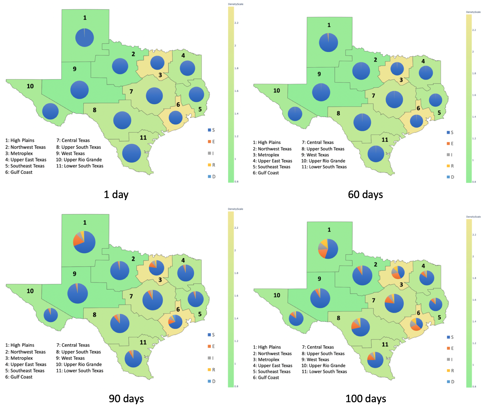
Figure 1: Prediction of Covid-19 spread over the state of Texas after 1, 60, 90, and 100 days from initial infection.

4.1 Forward prediction of epidemic dynamics

Here we illustrate the proposed model’s ability to predict the spatial and temporal dynamics of epidemic, assuming the parameter values displayed in Table 1. We ran the model for a period of 200 days. Fig 1 displays the results at day 1, day 60, day 90, and day 100. In this simulation, the epidemic is assumed to have originated in region 1 with only a few infective individuals, as can be seen in the upper left diagram of Fig 1. After 60 days, the pandemic has spread to other regions, but it is still very limited. However, after 90 days, i.e., only 30 days after the previous snapshot, the epidemic has spread much more widely, especially in the originating region 1, as well as regions with large populational density, e.g. region 3 and region 6, which is where Dallas and Houston are located, respectively. Finally, after only another 10 days, the number of infected individuals has almost doubled. These results show that the epidemic may be easier to control at an early stage. They also show that if the epidemic is allowed to run its course, it will spread at an exponential rate after a period of time. These predictions underscore the need for early-stage public health interventions, such as social distancing, mask wearing, or a limited lockdown in the critical originating region 1.

4.2 State and parameter estimation from synthetic data

In this section, we investigate the ability of the proposed maximum-likelihood adaptive filtering methodology in recovering both the hidden state and all unknown parameters of the pandemic from a synthetic time series of reported new cases and deaths. The synthetic data allow us to evaluate the performance of the methodology against the simulated ground truth.

In the first experiment, we assume that the parameter values (see Table 1) are known and we evaluate the ability of the filtering methodology to recover the hidden SEIRD state from the synthetic times series. Although in practice not all parameters would be known, this experiment allows us to evaluate the pure state estimation capabilities of the algorithm. Figure 2 displays the results over region 1 (the behavior was similar over all other regions). We can see that the maximum-likelihood adaptive filter can track the state evolution remarkably well.

Figure 2: State estimation in region 1 with all parameter values known.

In the second experiment, we remove the assumption that the infection rate, mean recovery time, and mortality rate parameters are known, and evaluate the performance of the methodology in recovering the values of these parameters. This is a difficult problem, since the states are also unknown, and the algorithm must perform simultaneous state and parameter estimation. Table 2 shows that the algorithm produced estimated parameter values that are close to the groundtruth values. Figure 3 displays state estimation results when the estimated parameters are plugged in for the unknown parameters. We can see that the results are not quite as good as the case where all parameters are known, in Figure 2, but the proposed methodology is still able to track the state evolution well.

Table 2: Parameter estimation with synthetic data.

Parameter	Groundtruth	Estimated Value
Infection rate ($\lambda_{S}$)	0.4	0.451
Mean recovery time ($1/\lambda_{R}$)	14 (days)	12.05 (days)
Mortality rate ($\lambda_{D}$)	0.01	0.0121

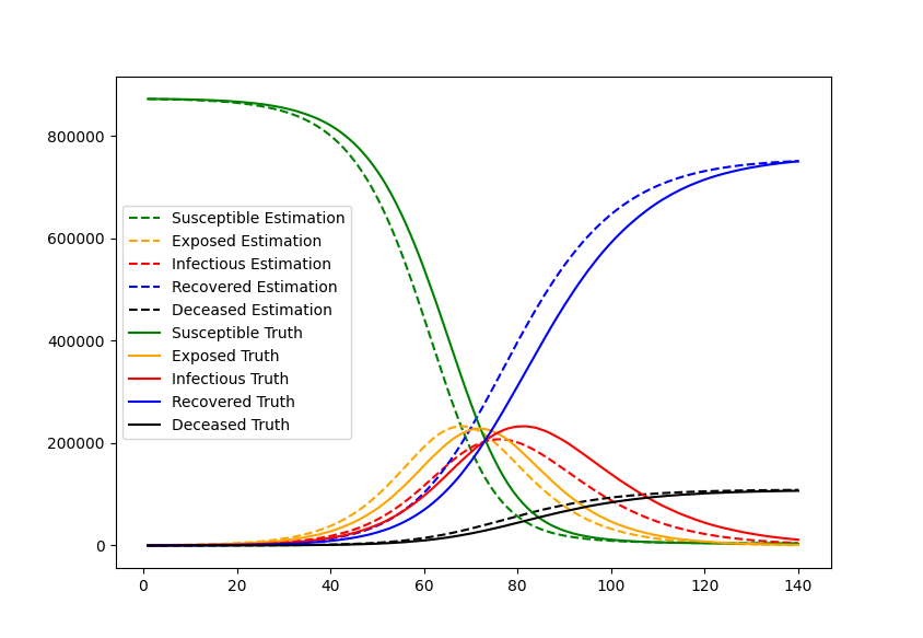
Figure 3: State estimation in region 1 using estimated parameter values.

4.3 State and Parameter Estimation using Johns Hopkins University Covid-19 Data

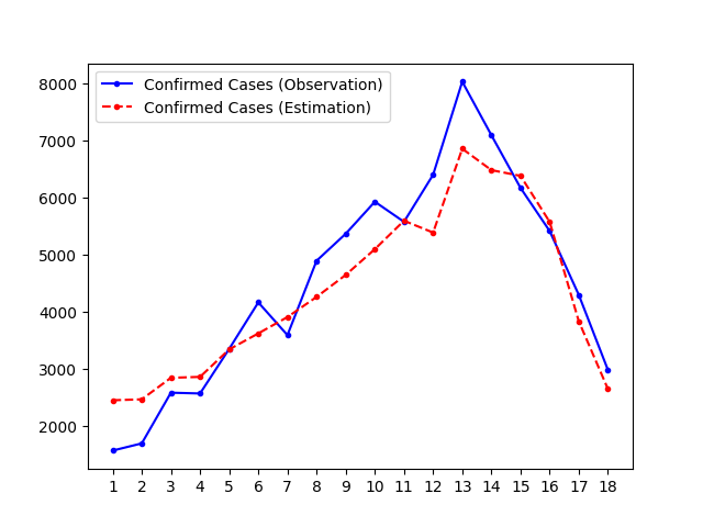
Figure 4: Prediction of new cases using JHU Covid-19 data over region 3. The blue line represents the actual observed data, the red dashed line are the predicted values in the time interval where the observed data is known.

In this experiment, we demonstrate the performance of the algorithm on Texas Covid-19 data from the Center for Systems Science and Engineering (CSSE) at Johns Hopkins University Dong E . Due to the presence of delayed reporting, there is often incorrect data in the early part of the week and corrections at the end of the week. To address this, we consider the time unit to be week, not day, and average the daily reported data (from Sunday to Saturday) to produce one data point for the week. The data used in this experiment is from the week of Oct 4th, 2020 to the week of Feb 1st, 2021, which is from the third (Fall 2020) wave of the COVID-19 epidemic in the United States. In this experiment, we only use data from four big regions (3, 6, 7, 8), which contain Dallas, Houston, Austin and San Antonio, which are the most reliable data available.

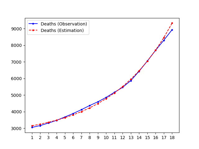
Figure 5: Prediction of cumulative deaths using JHU Covid-19 data over region 3. The blue line represents the actual observed data, the red dashed line are the predicted values in the time interval where the observed data is known.

We assume that only the test false positive rate, false negative rate and the mean incubation time are known. However, the value of the latter in Table 1 is based on a daily time unit, so here the value used is 10/7, or $\lambda_{E}=0.7$. All estimated rates obtained by the algorithm in this experiment can be divided by 7 in order to obtain daily rates.

Table 3: Estimated parameters for Texas Fall 2020 wave using JHU Covid-19 data

Parameter	Region 3	Region 6	Region 7	Region 8
Infection rate ($\lambda_{S}$)	0.16	0.16	0.16	0.16
Mean recovery time ($1/\lambda_{R}$)	9.92 (days)	10.52 (days)	10.85 (days)	10.95 (days)
Mortality rate ($\lambda_{D}$)	0.0111	0.00992	0.0135	0.0112

In addition, unlike in the experiment with synthetic data, we have no groundtruth for the states or parameters. In order to evaluate the performance of the algorithm, we use the estimated values of states and parameters to predict the time series of observed data and check its agreement with the actual JHU data. These plots are displayed in Figures 4 and 5 over region 3. They indicate that our model can accurately estimate the hidden states and unknown parameters. Table 3 displays the estimated values of the parameters. The value for the infection rate is the same over all regions, by assumption; however, Figures 4 and 5 provide evidence that this is a reasonable assumption.

4.4 Discussion

Compared with the standard SEIRD model, which assumes that the states of the epidemic can be observed directly, our stochastic state-space model realistically treats these states as hidden and only indirectly observed from the reported data. The proposed methodology is also able to incorporate detailed information about the testing procedure, such as false positive and false negative test rates and differential testing rate between symptomatic and asymptomatic patients. Our model provides a more accurate estimate of unknown/unobserved epidemiological parameters, such as the time-varying reproductive number, which are paramount for monitoring disease transmission dynamics and evaluating the effectiveness of ongoing control strategies. Moreover, our state-space model is more suitable for designing robust optimal control strategies and providing more accurate predictions of the future trends of an epidemic, based on the noisy reported time series data, than standard epidemic models.

Our model has limitations, which can be addressed by future work. First, our model does not consider vital dynamics such as birth and death from other causes. Provided that the model is run over a short interval of time, such as an isolated wave in the epidemic, the results will not be affected too much; in addition, new born play an insignificant role in Covid-19 spread. Second, we assume that individuals infected with COVID-19 will develop life-long immunity. Though some epidemiological data have indicated evidence of COVID-19 reinfections, in most cases immunity persist for at least eight months. Therefore, we believe that this assumption has a marginal impact on our results, provided once again that the model is run over a short enough time interval. Third, our model ignored the impact of age on COVID-19 epidemiological parameters such as infection rate, disease severity (symptomatic vs asymptomatic), mortality rate, recovery rate, and testing rate. Age-specific infection rate and disease-induced complications have been observed during the ongoing COVID-19 pandemic and considered to play an import role in disease transmission and the design of public health policies. Fourth, our model in it current form assumes that connection between the different regions can be modeled with a simple gravity commuting model Zipf (1946); Truscott and Ferguson (2012); Chen et al. (2021). This limitation can be addressed by using empirical population mobility data. Finally, Our model did not consider potential temporal changes of parameters over time, e.g. the mortality rate may be be high and recovery rate low at the beginning of an outbreak because of lack of effective treatments, or public behavior, such as social distancing and mask wearing, may vary over time. Also, in the case of the Fall 2020 wave, it is known that mass vaccination began at the end of this wave (December 2020), which very likely had a major impact in the disease transmission parameters. Hence, the estimated parameter values reflect average rates over the time interval in consideration.

5 Conclusion

We proposed a novel stochastic metapopulation state-space model for COVID-19 transmission, based on a discrete-time SEIRD model, which is able to estimate the hidden epidemic states and transmission parameters from a noisy time series of reported epidemiological data, by applying unscented Kalman filtering (UKF), Maximum Likelihood (ML) adaptive filtering, and metaheuristic optimization. We reported results from a comprehensive set of experiments, using synthetic data and real epidemic data to demonstrate that our model can estimate parameters and predict future trends accurately and effectively. The proposed framework was applied to the state of Texas in the United States, using data from the Center for Systems Science and Engineering (CSSE) at Johns Hopkins University. It can also be applied to any city/state/nation by providing the necessary time series data (e.g. reported cases, deaths, and testing rates). The proposed methodology may provide a valuable tool for revealing the current epidemic status through accurate estimated states and disease transmission parameters, improving the ability of authorities to make informed decisions on public health measures to contain the disease.

Conflict of interest

The authors declare that they have no conflicts of interest.

Appendix

Calculation of the covariance matrix Q of the process noise.

Covariance matrix $Q_{t}$ is a 5 by 5 square matrix giving the covariance between each pair of elements of the state process noise vector $(n^{t}_{S_{i}},n^{t}_{E_{i}},n^{t}_{I_{i}},n^{t}_{R_{i}},n^{t}_{D_{i}})$ for a specific region $i$ at time $t$.

Diagonal elements of the covariance matrix contain the variances of each variable, which are calculated as:

$$Var(n_{S_{i}}^{t})\,= Var\left(\Sigma_{j=1}^{G}N_{S_{i,j}}^{t}\right)$$ (33)

$$\,= \Sigma_{j}S_{i}^{t}\frac{c_{ij}\lambda_{S}I_{j}^{t}}{N_{j}}(1-\frac{c_{ij}\lambda_{S}I_{j}^{t}}{N_{j}})-\Sigma_{j_{1}}\Sigma_{j_{2}}S_{i}^{t}\frac{c_{ij_{1}}\lambda_{S}I_{j_{1}}^{t}}{N_{j_{1}}}\frac{c_{ij_{2}}\lambda_{S}I_{j_{2}}^{t}}{N_{j_{2}}},\hskip 8.53581ptj_{1}\neq j_{2}$$

$$\,= \Sigma_{j}S_{i}^{t}\frac{c_{ij}\lambda_{S}I_{j}^{t}}{N_{j}}-\Sigma_{j_{1}}\Sigma_{j_{2}}S_{i}^{t}\frac{c_{ij_{1}}\lambda_{S}I_{j_{1}}^{t}}{N_{j_{1}}}\frac{c_{ij_{2}}\lambda_{S}I_{j_{2}}^{t}}{N_{j_{2}}}$$

$$Var(n_{E_{i}}^{t})\,= Var\left(\Sigma_{j=1}^{G}N_{S_{i,j}}^{t}\right)+Var(N_{E_{i}}^{t})$$ (34)

$$\,= \Sigma_{j}S_{i}^{t}\frac{c_{ij}\lambda_{S}I_{j}^{t}}{N_{j}}-\Sigma_{j_{1}}\Sigma_{j_{2}}S_{i}^{t}\frac{c_{ij_{1}}\lambda_{S}I_{j_{1}}^{t}}{N_{j_{1}}}\frac{c_{ij_{2}}\lambda_{S}I_{j_{2}}^{t}}{N_{j_{2}}}+E_{i}^{t}\lambda_{E}(1-\lambda_{E})$$

$$Var(n_{I_{i}}^{t})\,= Var(N_{E_{i}}^{t})+Var(N_{R_{i}}^{t})+Var(N_{D_{i}}^{t})+2Cov(N_{R_{i}}^{t},N_{D_{i}}^{t})$$ (35)

$$\,= E_{i}^{t}\lambda_{E}(1-\lambda_{E})+I_{i}^{t}\lambda_{R}(1-\lambda_{R})+I_{i}^{t}\lambda_{D}(1-\lambda_{D})-2I_{i}^{t}\lambda_{R}\lambda_{D}$$

$$\,= E_{i}^{t}\lambda_{E}(1-\lambda_{E})+I_{i}^{t}(\lambda_{R}+\lambda_{D})(1-(\lambda_{R}+\lambda_{D}))$$

$$Var(n_{R_{i}}^{t})\,=\,Var(N_{R_{i}}^{t})=I_{i}^{t}\lambda_{R}(1-\lambda_{R})$$ (36)

$$Var(n_{D_{i}}^{t})\,=\,Var(N_{D_{i}}^{t})=I_{i}^{t}\lambda_{D}(1-\lambda_{D})$$ (37)

The off-diagonal elements contain the covariances of each pair of variables, which are calculated as:

$$Cov(n_{S_{i}}^{t},n_{E_{i}}^{t})\,=\,-Var(n_{S_{i}}^{t})$$ (38)

$$Cov(n_{E_{i}}^{t},n_{I_{i}}^{t})\,=\,-Var(N_{E_{i}}^{t})$$ (39)

$$Cov(n_{I_{i}}^{t},n_{R_{i}}^{t})\,= -Var(N_{R_{i}}^{t})-Cov(N_{R_{i}}^{t},N_{D_{i}}^{t})$$ (40)

$$\,= -I_{i}^{t}\lambda_{R}(1-\lambda_{R})+I_{i}^{t}\lambda_{R}\lambda_{D}$$

$$\,= -I_{i}^{t}\lambda_{R}(1-(\lambda_{R}+\lambda_{D}))$$

$$Cov(n_{I_{i}}^{t},n_{D_{i}}^{t})\,= -Var(N_{D_{i}}^{t})-Cov(N_{R_{i}}^{t},N_{D_{i}}^{t})$$ (41)

$$\,= -I_{i}^{t}\lambda_{D}(1-\lambda_{D})+I_{i}^{t}\lambda_{R}\lambda_{D}$$

$$\,= -I_{i}^{t}\lambda_{D}(1-(\lambda_{R}+\lambda_{D}))$$

$$Cov(n_{R_{i}}^{t},n_{D_{i}}^{t})\,=\,-I_{i}^{t}\lambda_{R}\lambda_{D}$$ (42)

The remaining elements will be zero.

Covariance of the observation noise (R)

Covariance matrix $R_{t}$ is a 2 by 2 square matrix giving the covariance between each pair of elements of the observation noise vector $({v_{p}}_{i}^{t},{v_{q}}_{i}^{t})$ for a specific region $i$ at time $t$.

Similarly, diagonal elements of the covariance matrix contain the variances of each variable, but all the off-diagonal elements will be zero.

$$var({v_{p}}_{i}^{t})\,= \varepsilon^{t}_{1}(1-\varepsilon^{t}_{3})(S_{i}^{t}+R_{i}^{t})\alpha(1-\alpha)+\varepsilon^{t}_{2}\varepsilon^{t}_{3}(S_{i}^{t}+R_{i}^{t})\alpha(1-\alpha)$$ (43)

$$+\varepsilon^{t}_{2}(1-\varepsilon^{t}_{4})I_{i}^{t}\beta(1-\beta)+\varepsilon^{t}_{1}(\varepsilon^{t}_{4}I_{i}^{t}+E_{i}^{t})\beta(1-\beta)$$

$$var({v_{q}}_{i}^{t})\,= D_{i}^{t}\beta(1-\beta)$$

References

- Degli Atti et al. [2008] Marta Luisa Ciofi Degli Atti, Stefano Merler, Caterina Rizzo, Marco Ajelli, Marco Massari, Piero Manfredi, Cesare Furlanello, Gianpaolo Scalia Tomba, and Mimmo Iannelli. Mitigation measures for pandemic influenza in italy: an individual based model considering different scenarios. PloS one, 3(3):e1790, 2008.
- Perez and Dragicevic [2009] Liliana Perez and Suzana Dragicevic. An agent-based approach for modeling dynamics of contagious disease spread. International journal of health geographics, 8(1):1–17, 2009.
- Hunter et al. [2018] Elizabeth Hunter, Brian Mac Namee, and John Kelleher. An open-data-driven agent-based model to simulate infectious disease outbreaks. PloS one, 13(12):e0208775, 2018.
- Chang et al. [2020] Sheryl L Chang, Nathan Harding, Cameron Zachreson, Oliver M Cliff, and Mikhail Prokopenko. Modelling transmission and control of the covid-19 pandemic in australia. Nature communications, 11(1):1–13, 2020.
- Chao et al. [2020] Dennis L Chao, Assaf P Oron, Devabhaktuni Srikrishna, and Michael Famulare. Modeling layered non-pharmaceutical interventions against sars-cov-2 in the united states with corvid. medRxiv, 2020.
- Koo et al. [2020] Joel R Koo, Alex R Cook, Minah Park, Yinxiaohe Sun, Haoyang Sun, Jue Tao Lim, Clarence Tam, and Borame L Dickens. Interventions to mitigate early spread of sars-cov-2 in singapore: a modelling study. The Lancet Infectious Diseases, 20(6):678–688, 2020.
- Kretzschmar et al. [2020] Mirjam Kretzschmar, Ganna Rozhnova, and Michiel van Boven. Isolation and contact tracing can tip the scale to containment of covid-19 in populations with social distancing. Available at SSRN 3562458, 2020.
- Kerr et al. [2020] Cliff C Kerr, Robyn M Stuart, Dina Mistry, Romesh G Abeysuriya, Gregory Hart, Katherine Rosenfeld, Prashanth Selvaraj, Rafael C Nunez, Brittany Hagedorn, Lauren George, et al. Covasim: an agent-based model of covid-19 dynamics and interventions. medRxiv, 2020.
- Balcan et al. [2010] Duygu Balcan, Bruno Goncontcalves, Hao Hu, José J Ramasco, Vittoria Colizza, and Alessandro Vespignani. Modeling the spatial spread of infectious diseases: The global epidemic and mobility computational model. Journal of computational science, 1(3):132–145, 2010.
- Dukic et al. [2012] Vanja Dukic, Hedibert F Lopes, and Nicholas G Polson. Tracking epidemics with state-space seir and google flu trends. Unpublished manuscript, 2012.
- Osthus et al. [2017] Dave Osthus, Kyle S Hickmann, Petrucontta C Caragea, Dave Higdon, and Sara Y Del Valle. Forecasting seasonal influenza with a state-space sir model. The annals of applied statistics, 11(1):202, 2017.
- Sebastian and Victor [2017] Elizabeth Sebastian and Priyanka Victor. A state space approach for sir epidemic model. International Journal of Difference Equations, 12(1):79–87, 2017.
- Keeling et al. [2020] Matt J Keeling, T Deirdre Hollingsworth, and Jonathan M Read. Efficacy of contact tracing for the containment of the 2019 novel coronavirus (covid-19). J Epidemiol Community Health, 74(10):861–866, 2020.
- Sameni [2020] Reza Sameni. Mathematical modeling of epidemic diseases; a case study of the covid-19 coronavirus. arXiv preprint arXiv:2003.11371, 2020.
- Godio et al. [2020] Alberto Godio, Francesca Pace, and Andrea Vergnano. Seir modeling of the italian epidemic of sars-cov-2 using computational swarm intelligence. International Journal of Environmental Research and Public Health, 17(10):3535, 2020.
- Kobayashi et al. [2020] Genya Kobayashi, Shonosuke Sugasawa, Hiromasa Tamae, and Takayuki Ozu. Predicting intervention effect for covid-19 in japan: state space modeling approach. BioScience Trends, 2020.
- Kermack and McKendrick [1927] William Ogilvy Kermack and Anderson G McKendrick. A contribution to the mathematical theory of epidemics. Proceedings of the royal society of london. Series A, Containing papers of a mathematical and physical character, 115(772):700–721, 1927.
- Hooker et al. [2011] Giles Hooker, Stephen P Ellner, Laura De Vargas Roditi, and David JD Earn. Parameterizing state–space models for infectious disease dynamics by generalized profiling: measles in ontario. Journal of The Royal Society Interface, 8(60):961–974, 2011.
- Zhong et al. [2009] ShaoBo Zhong, QuanYi Huang, and DunJiang Song. Simulation of the spread of infectious diseases in a geographical environment. Science in China Series D: Earth Sciences, 52(4):550–561, 2009.
- Rapolu et al. [2020] Taarak Rapolu, Brahmani Nutakki, T Sobha Rani, and S Durga Bhavani. A time-dependent seird model for forecasting the covid-19 transmission dynamics. medRxiv, 2020.
- Piccolomiini and Zama [2020] Elena Loli Piccolomiini and Fabiana Zama. Monitoring italian covid-19 spread by an adaptive seird model. MedRxiv, 2020.
- Korolev [2021] Ivan Korolev. Identification and estimation of the seird epidemic model for covid-19. Journal of econometrics, 220(1):63–85, 2021.
- Loli Piccolomini and Zama [2020] Elena Loli Piccolomini and Fabiana Zama. Monitoring italian covid-19 spread by a forced seird model. PloS one, 15(8):e0237417, 2020.
- Tiwari et al. [2020] Vipin Tiwari, Nandan Bisht, and Namrata Deyal. Mathematical modelling based study and prediction of covid-19 epidemic dissemination under the impact of lockdown in india. medRxiv, 2020.
- Zipf [1946] George Kingsley Zipf. The p 1 p 2/d hypothesis: on the intercity movement of persons. American sociological review, 11(6):677–686, 1946.
- Truscott and Ferguson [2012] James Truscott and Neil M Ferguson. Evaluating the adequacy of gravity models as a description of human mobility for epidemic modelling. PLoS Comput Biol, 8(10):e1002699, 2012.
- Chen et al. [2021] Qun Chen, Jiao Yan, Helai Huang, and Xi Zhang. Correlation of the epidemic spread of covid-19 and urban population migration in the major cities of hubei province, china. Transportation Safety and Environment, 3(1):21–35, 2021.
- Allen et al. [2020] William E Allen, Han Altae-Tran, James Briggs, Xin Jin, Glen McGee, Andy Shi, Rumya Raghavan, Mireille Kamariza, Nicole Nova, Albert Pereta, et al. Population-scale longitudinal mapping of covid-19 symptoms, behaviour and testing. Nature Human Behaviour, 4(9):972–982, 2020.
- Buitrago-Garcia et al. [2020] Diana Buitrago-Garcia, Dianne Egli-Gany, Michel J Counotte, Stefanie Hossmann, Hira Imeri, Aziz Mert Ipekci, Georgia Salanti, and Nicola Low. Occurrence and transmission potential of asymptomatic and presymptomatic sars-cov-2 infections: A living systematic review and meta-analysis. PLoS medicine, 17(9):e1003346, 2020.
- Wan and Van Der Merwe [2000] Eric A Wan and Rudolph Van Der Merwe. The unscented kalman filter for nonlinear estimation. In Proceedings of the IEEE 2000 Adaptive Systems for Signal Processing, Communications, and Control Symposium (Cat. No. 00EX373), pages 153–158. Ieee, 2000.
- Bastos Filho et al. [2008] Carmelo JA Bastos Filho, Fernando B de Lima Neto, Anthony JCC Lins, Antonio IS Nascimento, and Marilia P Lima. A novel search algorithm based on fish school behavior. In Systems, Man and Cybernetics, 2008. SMC 2008. IEEE International Conference on, pages 2646–2651. IEEE, 2008.
- Bastos-Filho and Nascimento [2013] CJA Bastos-Filho and DO Nascimento. An enhanced fish school search algorithm. In Computational Intelligence and 11th Brazilian Congress on Computational Intelligence (BRICS-CCI & CBIC), 2013 BRICS Congress on, pages 152–157. IEEE, 2013.
- Tan et al. [2020] Yukun Tan, Fernando Lima Neto, and Ulisses Braga-Neto. Pallas: Penalized maximum likelihood and particle swarms for inference of gene regulatory networks from time series data. IEEE/ACM Transactions on Computational Biology and Bioinformatics, 2020.
- Simon [2006] Dan Simon. Optimal state estimation: Kalman, H infinity, and nonlinear approaches. John Wiley & Sons, 2006.
- Särkkä [2013] Simo Särkkä. Bayesian filtering and smoothing. Number 3. Cambridge University Press, 2013.
- Ito and Xiong [2000] Kazufumi Ito and Kaiqi Xiong. Gaussian filters for nonlinear filtering problems. IEEE transactions on automatic control, 45(5):910–927, 2000.
- Wu et al. [2006] Yuanxin Wu, Dewen Hu, Meiping Wu, and Xiaoping Hu. A numerical-integration perspective on gaussian filters. IEEE Transactions on Signal Processing, 54(8):2910–2921, 2006.
- Kokkala et al. [2015] Juho Kokkala, Arno Solin, and Simo Särkkä. Sigma-point filtering and smoothing based parameter estimation in nonlinear dynamic systems. arXiv preprint arXiv:1504.06173, 2015.
- Asai [2020] Takashi Asai. Covid-19: accurate interpretation of diagnostic tests—a statistical point of view, 2020.
- [40] Gardner L Dong E, Du H. An interactive web-based dashboard to track covid-19 in real time. Lancet Inf Dis., 20(5):533–534. doi:10.1016/S1473-3099(20)30120-1.