Variational Quantum Anomaly Detection: Unsupervised mapping of phase diagrams on a physical quantum computer

Abstract

One of the most promising applications of quantum computing is simulating quantum many-body systems. However, there is still a need for methods to efficiently investigate these systems in a native way, capturing their full complexity. Here, we propose variational quantum anomaly detection, an unsupervised quantum machine learning algorithm to analyze quantum data from quantum simulation. The algorithm is used to extract the phase diagram of a system with no prior physical knowledge and can be performed end-to-end on the same quantum device where the system is simulated on. We showcase its capabilities by mapping out the phase diagram of the one-dimensional extended Bose Hubbard model with dimerized hoppings, which exhibits a symmetry protected topological phase. Further, we show that it can be used with readily accessible devices today by performing the algorithm on a real quantum computer.

I Introduction

Since the discovery of Shor’s algorithm Shor (1994), there have been many attempts to leverage the power of quantum computers to outperform classical computers Nielsen and Chuang (2010). One of the most promising near- and far-term applications is simulating quantum many-body systems. Universal quantum simulation algorithms like phase estimation Kitaev (1995); Nielsen and Chuang (2010), or adiabatic quantum computation Farhi et al. (2000) require quantum fault-tolerance Aharonov and Ben-Or (1999), that is, the ability to reliably correct errors that occur during the quantum computation. With recent experimental advancements in quantum error correction Semeghini et al. (2021); Satzinger et al. (2021), there is hope that quantum fault-tolerance can one day be reached. Currently, we only have access to noisy intermediate-scale quantum (NISQ) devices Preskill (2018). There are several proposals for algorithms on these devices Benedetti et al. (2019); Bharti et al. (2021) like the variational quantum eigensolver (VQE) Peruzzo et al. (2014), the quantum approximate optimization algorithm (QAOA) Farhi et al. (2014), or the quantum autoencoder Romero et al. (2017); Bravo-Prieto (2021), that employ parameterized circuits which are optimized through a classical feedback loop, typically with gradient based methods McClean et al. (2015); Stokes et al. (2019); Cerezo et al. (2020a). These approaches can suffer from so-called Barren Plateaus, the phenomenon of an exponentially vanishing gradient of the loss function McClean et al. (2018). In practice, this issue occurs for large systems but can be avoided by using shallow circuits and local cost functions Cerezo et al. (2020b). While gradient-free optimization does not solve the Barren Plateau problem Arrasmith et al. (2021), other proposals give hope for large-scale and deep variational quantum circuits Pesah et al. (2021); Volkoff and Coles (2021).

With the rise of deep learning in the 2010s, the term quantum machine learning was mostly used to refer to leveraging quantum computers for linear algebra tasks such as matrix inversion in sub-polynomial time via the Harrow-Hassidim-Lloyd algorithm Harrow et al. (2008); Biamonte et al. (2017). One famous use-case was the quantum recommendation system algorithm with an exponential quantum speed-up at the time Kerenidis and Prakash (2016), which inspired classical analogs of the algorithm with the same, sub-polynomial, complexity (termed as quantum-inspired machine learning algorithms) Tang (2018). Today, quantum machine learning refers to using quantum circuits as neural networks Pérez-Salinas et al. (2020), or kernel functions Schuld (2021) to perform classical machine learning tasks like supervised learning Farhi and Neven (2018); Rebentrost et al. (2013). There are cases, where quantum models have provable advantages over classical models Liu et al. (2020), but it has been argued that these instances are special cases and no quantum speed up is to be expected for quantum machine learning with classical data Kübler et al. (2021).

On the other hand, applying classical machine learning to quantum physics has been a great success story Carleo et al. (2019), most prominently for the classification and mapping of phase diagrams Carrasquilla and Melko (2016); van Nieuwenburg et al. (2016); Huembeli et al. (2018). These methods rely on classical data and are therefore restricted by the available classical simulation methods. With physical devices surpassing system sizes that are classically tractable Arute et al. (2019), there is need for methods to investigate physical quantum states with quantum computers.

In this paper, we propose a quantum machine learning algorithm for quantum data. The data are ground states of quantum many-body systems that are prepared by a quantum simulation subroutine and serve as the input for Variational Quantum Anomaly Detection (VQAD). Our quantum anomaly detection scheme belongs to the category of variational quantum algorithms where the circuit learns characteristic features of the input state . This can in principle be leveraged for obtaining physical insights of the system from training Iten et al. (2018) and is in contrast to previous proposals that are based on kernel methods (one-class support vector machines) Liu and Rebentrost (2017); Liang et al. (2019). In the present study, we use it to map out an unknown phase diagram of a system without requiring knowledge about the order parameter or the number and location of the different phases.

In anomaly detection, the task is to differentiate normal data from anomalous data, opposed to supervised learning tasks, where a fixed set of classes with labels for training are differentiated. On the other hand, the task of anomaly detection requires an anomaly syndrome, i.e., an observable that is trained to be of a certain value (typically $0$) when normal data is input, and be significantly larger for anomalous data it is tested on. In classical machine learning, anomaly detection has already been used to extract phase diagrams in an unsupervised fashion from simulated and experimental data Kottmann et al. (2020); Käming et al. (2021); Kottmann et al. (2021a). VQAD allows us to perform anomaly detection directly on a quantum computer, and, with programmable devices readily available, we demonstrate it experimentally on a real device.

II Proposal

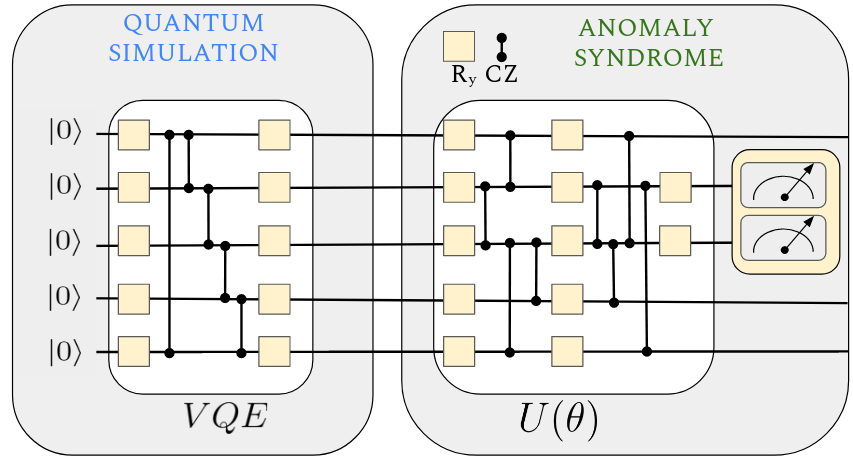
Figure 1: Overview of our proposal. First, the quantum states are prepared via VQE. Then, they are processed through the anomaly syndrome, consisting of a parameterized unitary $U(\theta)$ and a measurement of a subset of qubits, referred to as trash qubits. $R_{y}$ indicates a parameterized y-axis rotation and $CZ$ a (fixed) controlled-z gate.

The task of detecting anomalies in ground states of quantum many-body Hamiltonians can be loosely divided into two sub tasks: Preparing the ground state for specific Hamiltonian parameters, and computing an anomaly syndrome indicating whether the state corresponds to a normal example or an anomaly. An overview of our proposed algorithm is shown in Fig. 1. The problem of state preparation on quantum computers is one of ongoing research, and in principle, one can use any state preparation subroutine for preparing the ground state. Here, we choose the Variational Quantum Eigensolver (VQE) as it has the lowest hardware requirements while achieving reliable results on current devices Peruzzo et al. (2014); Kandala et al. (2017). The VQE algorithm iteratively minimizes the expectation value of a Hamiltonian with the ansatz circuit to find the ground state by optimizing the parameters of the circuit via a quantum-classical feedback loop. We choose a minimal ansatz as depicted in Fig. 1 that is sufficient for simulating the Ising Hamiltonian discussed in Sec. III.2. A shallow ansatz allows us to run both, the quantum simulation, and the quantum anomaly detection on real noisy devices. For more complex systems, the problem of finding a suitable hardware efficient ansatz can be addressed for example by the adaptive VQE algorithm Grimsley et al. (2019). In this work we employed the VQE implementation provided by the Qiskit library Abraham et al. (2019) and optimized it using simultaneous perturbation stochastic approximation (SPSA) Spall (1998). For all technical details we refer to App. A.

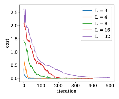
Figure 2: Scaling of the training cost of the anomaly syndrome ansatz. Successful training of the proposed anomaly syndrome ansatz for $L\in\{3,4,8,16,32\}$ corresponding to $n_{t}\in\{1,2,3,4,5\}$ trash qubits (and therefore $n_{t}$ circuit layers). The result for $L=32$ was obtained through MPS simulations with a maximal bond dimension of BD = $100$. We used $1000$ shots per evaluation and achieve a perfect cost value of $0.00$ for all system sizes, however the run for $L=32$ shown here finished at $0.03$.

Once the ground state is prepared on the quantum device a subsequent circuit serves as the anomaly syndrome. Our circuit ansatz is inspired by the recently proposed quantum auto-encoder, which similar to its classical counterpart can be used for compression of classical and quantum data Romero et al. (2017); Bravo-Prieto (2021). It is composed of several layers each consisting of parameterized single qubit y-rotations and controlled-z gates. After the final layer a predefined number $n_{t}$ of trash qubits is measured in the computational basis. The objective is to decouple the trash qubits from the rest of the system, effectively compressing the original ground state into a smaller number of qubits. The circuit parameters are then optimized to faithfully compress states that are considered normal. However, when the optimized circuit is tested on anomalous states not seen during training, it is expected that the circuit fails to decouple the trash qubits from the rest of the system. To quantify the degree of decoupling we use the Hamming distance $d_{H}$ of the trash qubit measurement outcomes to the $|0\rangle^{\otimes n_{t}}$ state, i.e., the number of 1s in a bit-string of measurement outcomes Bravo-Prieto (2021). The cost function $C$ can then be defined as the Hamming distance averaged over several circuit evaluations $C=1/N\sum_{i}^{N}d_{Hi}$, where $N$ is the number of performed measurements or shots. The cost function can also be rewritten in terms of expectation values of local Pauli-z operators $Z_{j}$

$$C=\frac{1}{N}\sum_{i=1}^{N}d_{Hi}=\frac{1}{2}\sum_{j=1}^{n_{t}}\left(1-\left\langle Z_{j}\right\rangle\right).$$ (1)

The VQAD circuit achieves perfect compression if the trash qubits are fully disentangled from the remaining qubits and mapped into the pure $|0\rangle^{\otimes n_{t}}$ state resulting in a cost equal to zero.

The specific circuit ansatz for the anomaly syndrome is shown in Fig. 1 for the case of $n_{t}=2$ trash qubits. Each layer of the circuit starts with parameterized single-qubit y-rotations applied to every qubit followed by a sequence of entangling controlled-z gates. The currently available NISQ devices are inherently noisy and the computations are subject to gate errors. To minimize the number of two-qubit gates we apply the controlled-z gates only between trash qubits and non-trash-qubits as well as between trash qubits themselves instead of an all-to-all entangling map Bravo-Prieto (2021). This entangling map is physically motivated as the goal of the circuit is to disentangle the trash qubits from the rest, with the trash qubits resulting in the $|0\rangle^{\otimes n_{t}}$ state. In a single layer each non-trash qubit will be coupled to exactly one trash qubit. This entangling scheme is repeated in the subsequent layers until every non-trash qubit has been coupled to each trash qubit exactly once, i.e. the number of layers of the circuit is equal to $n_{t}$. After the final layer, additional single-qubit y-rotations act on the trash qubits before they are measured.

Barren Plateaus are the fundamental obstacle prohibiting training of variational circuits with increasing numbers of qubits McClean et al. (2018). It was previously shown that using local cost functions and circuits featuring a number of layers scaling at most logarithmically in the system size can prevent the occurrence of Barren Plateaus Cerezo et al. (2020b). Additionally for realistic devices, gate errors lead to decoherence, making quantum simulation on real devices a challenging task even for small systems and low depths Cervera-Lierta (2018). The former calls for a minimal number of layers while the latter calls for a minimal number of gates overall. Therefore, we seek a minimal solution for our variational circuit that we want to implement on a readily available NISQ-era quantum computer. On the other hand, it is desirable to have an ansatz as general as possible to be able to capture a wide range of problems (see circuit complexity Bernstein and Vazirani (1997); Brandão et al. (2019)).

For the anomaly syndrome in this paper, we propose an ansatz that aims at compromising between being general enough to compress the ground states of the investigated systems while still being trainable. One way to make our circuit scalable for larger systems is to choose the number of trash qubits $n_{t}=\left\lfloor\log_{2}L\right\rfloor$, where $L$ is the total number of qubits. Together with the fact that our cost function is composed of only local operators, the training is expected to not suffer from Barren Plateaus. We empirically confirm successful trainability, i.e., achieving a cost of $0.0$ for ground states of the systems discussed later in the manuscript, for $L\in\{3,4,8,16,32\}$, corresponding to $n_{t}\in\{1,2,3,4,5\}$, respectively. In Fig. 2, a ground state of the Ising model Eq. 5 at $g_{x},g_{z},J=(0.3,0,1)$ is taken as a realistic example and we can confirm successful trainability in all cases.

Note that in principle the trash qubits can be placed anywhere in the circuit, however, when performing computations on a real quantum device it proved advantageous to explicitly take the qubit connectivity structure of the device into account in order to reduce the number of required SWAP operations. Specifically here, we placed the trash qubits in the middle of the IBMQ devices.

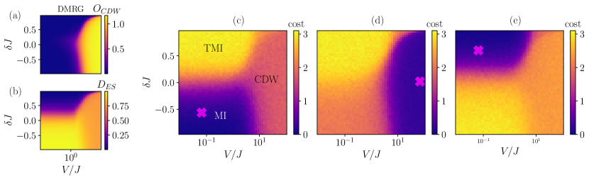
Figure 3: (a)-(b) Phase diagram of the DEBHM from Eq. (2) using (a) the order parameter $O_{CDW}$ defined in Eq. (3), and (b) the degeneracy of the entanglement spectrum, $D_{ES}$, defined in Eq. (4). The results were obtained from DMRG simulations for a system of length $L=12$ at half filling $\bar{n}=0.5$. We fix the maximum bond dimension $BD=50$ and the maximum number of bosons per site to $n_{0}=1$. (c)-(e) Cost/anomaly syndrome of a VQAD trained on a single ground state (indicated by a cross) of the $L=12$ DEBHM using $n_{t}=6$ trash qubits in the (c) MI phase, (d) CDW phase, and (e) TMI phase. The cost at each data point is the Hamming distance averaged over 1000 measurement shots using an ideal quantum device simulator.

The training and inference procedure is identical to the classical anomaly detection schemes for mapping out phase diagrams Kottmann et al. (2020). In the first step, one randomly chooses a training region in the phase diagram that represents normal data, which is an arbitrary definition. Note that no prior knowledge about the phase diagram is therefore required. The circuit representing the anomaly syndrome is then trained on ground states of the training region, and tested on the whole phase diagram. States in the same phase as the training data are normal and can be disentangled, leading to a low cost. Anomalous states can be inferred through an increase in the cost function signaling that the corresponding ground state cannot be disentangled by the optimized circuit. From the resultant cost profile, we can deduce the phase boundary between the phase the circuit has been trained on and any other phases in the diagram. This procedure is then repeated by training in the anomalous region from the previous iteration until all phase boundaries are found. An example is provided in Fig. 3.

Anomaly detection is a semi-supervised learning task. The setting is typically that one is provided with one class of data that is well known, normal data, and aims at finding outliers of that distribution, anomalous data. An archetypical example is credit card fraud where a big database of normal transactions is provided and one aims at finding fraudulent ones. We consider anomaly detection semi-supervised as labeled data (x, “normal”) is provided for training while (x, “anomalous”) is to be inferred. Here, however, we arbitrarily define (x, “normal”) and iteratively find the different classes (phases of matter). The definition of (x, “normal”) is arbitrary and does not necessitate prior knowledge. Furthermore, it is merely a means to an end to find the different classes. In that sense, the way anomaly detection is used to map out the phase diagram can be regarded as an unsupervised learning method.

Note that in previous works, where the same task has been tackled with classical machine learning techniques, it has been shown that a single ground state was sufficient to successfully train the model Kottmann et al. (2021a). This feature stems from the fact that ground states within the same phase share similar properties and there is very little variance when changing the physical parameters inside one phase. We observe this feature also in the training of the VQAD.

III Results

III.1 Simulations with ideal quantum data

In order to test the performance of VQAD, we first study the one-dimensional extended Bose Hubbard model with dimerized hoppings (DEBHM) Sugimoto et al. (2019),

$$H = -\sum_{i=1}^{L-1}(J+\delta J(-1)^{i})(b_{i}^{\dagger}b_{i+1}+\text{h.c.})+$$ (2)

$$+\frac{U}{2}\sum_{i}^{L}n_{i}(n_{i}-1)+V\sum_{i}^{L-1}n_{i}n_{i+1},$$

where $b^{\dagger}_{i}(b_{i})$ is the bosonic operator representing the creation(annihilation) of a particle at site $i$ of a lattice of length $L$. The tunneling amplitudes $J-\delta J$ $(J+\delta J)$ indicate hopping processes on odd (even) links connecting nearest-neighbor sites, while $V$ represents the nearest-neighbor (NN) repulsion. Here, we take the hardcore boson limit, i.e. the on-site repulsion $U/J\rightarrow\infty$, such that the local Hilbert space is two-dimensional and each site can only accommodate $0$ or $1$ bosons. This model can be effectively mapped into a spin-$1/2$ system Wang et al. (2013).

Previous studies of the DEBHM model at half filling ($\bar{n}=0.5$) have demonstrated the existence of three distinct phases Sugimoto et al. (2019). For small and intermediate values of $V/J$ and $\delta J>0$, we find a topological Mott insulator (TMI) displaying features analogous to a symmetry protected topological phase appearing in the dimerized spin-1/2 bond-alternating Heisenberg model Wang et al. (2013). On the other hand, for negative values of $\delta J$ we expect a trivial Mott insulator (MI), while in the regime where the nearest-neighbor repulsion dominates, a charge density wave (CDW) appears.

In Fig. 3(a)-(b), we study the phase diagram of the model in Eq. (2) in terms of the parameters $\delta J$ and $V/J$, using the density matrix renormalization group algorithm (DMRG) Schollwöck (2011); White (1992); Hauschild and Pollmann (2018). In order to differentiate between the Mott insulating phases and the CDW, one can compute the CDW order parameter

$$O_{CDW}=\sum_{i=1}^{L/2}(-1)^{i}\delta n_{i},$$ (3)

which detects staggered patterns in the density. In Fig. 3(a) we report a vanishing value of $O_{CDW}$ everywhere but in the region with large values of $V/J$, which corresponds to the CDW . To characterize the TMI we study the entanglement spectrum (ES), which is expected to be doubly degenerate in a topologically non-trivial phase Pollmann et al. (2010) due to the existence of edge states. The entanglement spectrum $\{\lambda_{i}\}$ is defined in terms of the positive real-valued Schmidt coefficients $\{\alpha_{i}\}$ of a bipartite decomposition of the system by $\alpha_{i}^{2}=\exp(-\lambda_{i})$. We determine its degeneracy using

$$D_{ES}=\sum_{i}(-1)^{i}e^{-\lambda_{i}}.$$ (4)

In Fig. 3(b), we show that the quantity $D_{ES}$ vanishes only for small NN interaction strengths $V$ and positive values of $\delta J$, which correponds to the TMI. The trivial MI and CDW phases do not show a degeneracy and hence do not host topological edge states.

In the following, we test the capabilities of the VQAD with ideal states obtained from DMRG simulations. The anomaly syndrome is trained using a single representative ground state within one of the phases such that the cost measured at the trash qubits is minimised and the states of this phase can be efficiently compressed by the circuit. Afterwards, the trained circuit processes all states from the full phase diagram, ideally with similarly low cost in the same phase and significantly higher cost in other phases.

In Fig. 3(c)-(e) we show the resultant cost diagram for three circuits, each optimized at a different point in the phase diagram. Indeed, ground states outside of the training phase give rise to a large cost and hence are correctly classified by the VQAD as anomalous. Surprisingly, a single ground state example (indicated by the cross) was sufficient to successfully train the VQAD and infer all three phases. Similar results were recently reported for the case of classical anomaly detection using neural network auto-encoders Kottmann et al. (2021a).

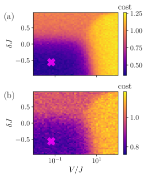
Figure 4: Cost of a VQAD trained on a single ground state in the MI phase (marked by the cross) of the DEBHM with $L=12$ sites and $n_{t}=2$ trash qubits. The gates of the VQAD circuit are subject to depolarizing noise with $p_{\text{err}}=0.001$ (single-qubit gates) and (a) $p_{\text{err}}=0.01$, (b) $p_{\text{err}}=0.07$ (two-qubit gates). The chosen values are motivated by the error probabilities of real devices.

To demonstrate the robustness of the VQAD against noise present in currently available NISQ devices we apply a depolarizing noise channel after each gate with error probabilities $p_{\text{err}}=0.001$ (single-qubit gates) and $p_{\text{err}}=0.01,0.07$ (two-qubit gates) and show two exemplary cost profiles of the trained anomaly detector in Fig. 4. Since the noise becomes more prominent with larger circuit depths, we used the two-layer VQAD circuit ansatz with only two trash qubits in this case. While it is not possible to reach a cost of zero in the training phase, the optimization still converges and all three phases can be successfully inferred. Hence, this suggests that even if the VQAD is not able to fully disentangle the trash qubits, the phase diagram can still be recovered from the resultant cost profile.

III.2 Experiments on a real quantum computer

We have seen that with ideal quantum data, VQAD can map out non-trivial phase diagrams including topologically non-trivial phases with and without noise in the anomaly syndrome. Next, we discuss its performance in real-noise simulations, that is with noise profiles and qubit connectivities from a real quantum device. Furthermore, we perform the quantum simulation subroutine, i.e., the ground state preparation via VQE, on the same circuit. For this task, we consider the paradigmatic transverse longitudinal field Ising (TLFI) model Fogedby (1978)

$$H=J\sum_{i=1}^{L}Z_{i}Z_{i+1}-g_{x}\sum_{i=1}^{L}X_{i}-g_{z}\sum_{i=1}^{L}Z_{i},$$ (5)

where $X_{i},Z_{i}$ are the Pauli matrices on site $i$, $J$ is the coupling strength, and $g_{x},g_{z}$ are the transverse and longitudinal fields, respectively. For $g_{z}=0$ the model is exactly solvable and shows a quantum phase transition from a ferromagnetic (antiferromagnetic) phase for $g_{x}/J<1$ and $J$ negative (positive) to a paramagnetic one for $g_{x}/J>1$ Sachdev (2007). In the following we set $J=1$ and vary the longitudinal and transverse fields. In this regime the model is not exactly solvable and the phase diagram has been extensively studied numerically Sen (2000); Ovchinnikov et al. (2003). The antiferromagnet-paramagnet quantum phase transition is best characterized by the order parameter which in this case is the staggered magnetization

$$\hat{S}=\sum_{i=1}^{L}(-1)^{i}\frac{Z_{i}}{L}.$$ (6)

We simulate the ground states of the Hamiltonian in Eq. 5 using VQE for $L=5$. On a noisy device, long-range entangling gates are performed by consecutive local two-qubit gates (SWAP operation), increasing the actual circuit depth. A large number of consecutive gates leads to decoherence due to gate errors and destroys the results. With the circuit presented in Fig. 1 for the VQE subroutine, we found a trade-off between expressibility and noise tolerance with a circular entanglement distribution and only one layer. Additionally, we performed measurement error mitigation Bravyi et al. (2021), which can further improve the results of the cost function as seen in Fig. 7 in App. A.

For small values of $g_{x}$ and $g_{z}$, in the ferromagnetic ordered phase, the ground states $\psi\simeq\ket{10101}$ ($\langle\hat{S}\rangle=1$) and $\psi\simeq\ket{01010}$ ($\langle\hat{S}\rangle=-1$) have a similar energy, which is why the optimization can get stuck in local minima. Hence, in the ordered phase, VQE can converge to both a state with positive or negative staggered magnetization, or an equal superposition of the two as can be seen in Fig. 5(a). The VQAD simulation results in Fig. 5(b) show a perfect correlation between positive $\braket{\hat{S}}$ and low cost, and vice versa, negative $\braket{\hat{S}}$ and high cost - which, intuitively, can be expected . The disordered phase is detected from the plateau of high cost ($\sim 1$).

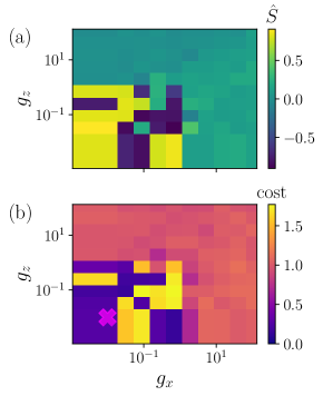
Figure 5: Real-noise simulations of the staggered magnetization $\hat{S}$ (a) and the anomaly syndrome (b) for the TLFI model. We trained the anomaly syndrome in the ordered phase on a state with positive $\hat{S}$, indicated by the purple cross. Inside the ordered phase, there is a perfect correlation between low cost states for positive $\hat{S}$, and very high cost where VQE converged to a negative $\hat{S}$. The paramagnetic phase is detected by a plateau in the anomaly syndrome.

We see that VQAD also performs well under realistic conditions, so we next test the algorithm on a physical device. For this task, we use the $L=5$ qubits on ibmq_jakarta Bravyi et al. (2021). To avoid jumps in the staggered magnetization in the ordered phase and improve convergence of the VQE optimization, we reuse already optimized parameters at neighboring points in the phase diagram as a good initial guess. Due to a large computation time overhead per execution on the real device, we additionally prepared pre-optimized parameters for both subroutines from a realistic noisy simulation, and use these as initial guesses for the optimization on the device. We found that for computing the staggered magnetization it is actually not necessary to re-run the VQE optimization on the physical device, and we can achieve faithful results by directly using the optimized parameters from the simulation as seen in Fig. 6. The resulting cost values for the optimized circuit, plotted in Fig. 6, clearly distinguish the two phases, with the cost from the experiment showing solely an almost constant offset compared to the noisy simulation.

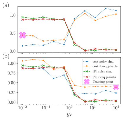
Figure 6: Real device VQAD experiments: We show the order parameter $\hat{S}$ compared to the VQAD results both for execution on ibmq_jakarta and noisy simulators with the same noise profile. We trained on a single ground state in the ordered (a) and paramagnetic (b) phase. For sampling $\hat{S}$, we use the same parameters for the VQE circuit in simulation and experiment. All values for $\hat{S}$ in the paramagnetic phase are negative, hence, for better visualization we plot its absolute value $|\hat{S}|$. For training the anomaly syndrome, the optimized parameters from the simulation are taken as an initial guess.

IV Outlook

We showed that our proposed algorithm is capable of mapping out complex phase diagrams, including topologically non-trivial phases. We further demonstrated that the algorithm also works in realistic scenarios for both real-noise simulations and on a real quantum computer. Hence, we provide a tool to experimentally explore phase diagrams in future quantum devices, which will be especially useful when physical devices surpass the limit of what can be classically computed.

Currently, the main bottleneck of VQAD is the presence of noise in real devices. We were able to improve our anomaly detection scheme by employing measurement error mitigation and adopting the circuits according to the physical device. These results are promising, and with current efforts on enhancing device performances, error mitigation and circuit optimization strategies in the community, we are hopeful to see even further improvements soon.

In this work we focused on using VQAD to extract the phase diagram of quantum many-body systems. A possible future extension would be to apply it to the problem of entanglement witnessing and certification in many-body scenarios without tomography. Furthermore, the use of an autoencoder-like architecture has the advantage over kernel-based schemes in that there exists tools of interpreting the feature space in classical autoencoders to gain physical insights Iten et al. (2018), which can be a possible future extension for the quantum case discussed here.

Acknowledgments

The authors thank D. González-Cuadra, L. Barbiero and U. Bhattacharya for discussions on the extended Bose Hubbard model and A. Dauphin, J. Bowles and M. Lewenstein for valuable feedback on the manuscript.

This work was supported by the European Union’s Horizon 2020 research and innovation programme under the Marie Sklodowska-Curie grant agreement No 713729 (K.K.). This work was supported by OIST Graduate University and we are grateful for the help and support provided by the Scientific Computing and Data Analysis Section of the Research Support Division at OIST. N.B. acknowledges support from a “la Caixa” Foundation (ID 100010434) fellowship. The fellowship code is LCF/BQ/DI20/11780033. We acknowledge support from ERC AdG’s NOQIA and CERQUTE, Spanish MINECO (FIDEUA PID2019-106901GB-I00/10.13039 / 501100011033, FIS2020-TRANQI, Severo Ochoa CEX2019-000910-S and Retos Quspin), the Generalitat de Catalunya (CERCA Program, SGR 1341, SGR 1381 and QuantumCAT), Fundacio Privada Cellex and Fundacio Mir-Puig, MINECO-EU QUANTERA MAQS (funded by State Research Agency (AEI) PCI2019-111828-2 / 10.13039/501100011033), EU Horizon 2020 FET-OPEN OPTOLogic (Grant No 899794), and the National Science Centre, Poland-Symfonia Grant No. 2016/20/W/ST4/00314.

We acknowledge the use of IBM Quantum services for this work. The views expressed are those of the authors, and do not reflect the official policy or position of IBM or the IBM Quantum team.

Author contributions

KK and FM contributed equally to this work.

KK initiated and managed the project, performed the VQAD simulations for the TLFI model, and was in charge of the ansatz scaling and the experiments on the physical device.

FM was in charge of the implementation in Python/Qiskit, worked on the TLFI model and performed the VQAD simulations for the DEBHM.

JF was in charge of DEBHM, the DMRG simulations and performed VQE simulations for the TLFI model.

NB worked on the implementation of the TLFI model and performed VQE simulations, and worked on error mitigation in noisy simulations.

All authors contributed to the discussions and the writing of the manuscript.

Appendix A Technical details

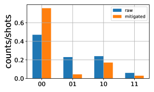
Figure 7: Comparison of the trash qubit measurement outcomes with and without measurement error mitigation. The anomaly syndrome circuit has been trained with and without error mitigation on a ground state of the TLFI model in the ordered phase in real-noise simulations. Ideally, all of the $1000$ shots would result in the $00$ bit string. By mitigating the measurement errors we improve the results towards this desired outcome.

The code to run the simulations and experiments discussed in the main text can be found in our repository on GitHub Kottmann et al. [2021b]. The optimization of the circuit parameters was performed using simultaneous perturbation stochastic approximation (SPSA) Spall [1998], Kandala et al. [2017]. To obtain the results presented in Fig. 3 of Sec. III.1, a VQAD circuit ansatz composed of 6 layers (6 trash qubits) was employed resulting in $6L+6$ parameters. For the noisy simulations and real-device execution discussed in Sec. III.2, we used the ansatz in Fig. 1, counting $2L$ and $2L+2$ parameters for the quantum simulation and anomaly syndrome, respectively. In classical real-noise simulations, we used $500$ VQE optimization iterations for the initial ground state optimization, and $200$ iterations for all subsequent optimizations where the previously optimized parameters were taken as initial guesses. For the anomaly detection circuit, we found converged results with less than $100$ optimization iterations. As an example, calculating the expectation value of the magnetization takes roughly $2-10$ seconds on a commercial laptop (here: i7-4712HQ), while the real-device execution takes about $30$ seconds. Furthermore, we used measurement error mitigation Bravyi et al. [2021] provided by the Qiskit library to improve the results of the VQAD simulations in the presence of noise as illustrated in Fig. 7.

References

- Shor [1994] P.W. Shor. Algorithms for quantum computation: discrete logarithms and factoring. In Proceedings 35th Annual Symposium on Foundations of Computer Science, pages 124–134, 1994. doi: 10.1109/SFCS.1994.365700.
- Nielsen and Chuang [2010] Michael A. Nielsen and Isaac L. Chuang. Quantum Computation and Quantum Information: 10th Anniversary Edition. Cambridge University Press, 2010. doi: 10.1017/CBO9780511976667.
- Kitaev [1995] A. Yu. Kitaev. Quantum measurements and the Abelian Stabilizer Problem. nov 1995. URL http://arxiv.org/abs/quant-ph/9511026.
- Farhi et al. [2000] Edward Farhi, Jeffrey Goldstone, Sam Gutmann, and Michael Sipser. Quantum Computation by Adiabatic Evolution. jan 2000. URL http://arxiv.org/abs/quant-ph/0001106.
- Aharonov and Ben-Or [1999] Dorit Aharonov and Michael Ben-Or. Fault-Tolerant Quantum Computation With Constant Error Rate. SIAM Journal on Computing, 38(4):1207–1282, jun 1999. URL http://arxiv.org/abs/quant-ph/9906129.
- Semeghini et al. [2021] Giulia Semeghini, Harry Levine, Alexander Keesling, Sepehr Ebadi, Tout T. Wang, Dolev Bluvstein, Ruben Verresen, Hannes Pichler, Marcin Kalinowski, Rhine Samajdar, Ahmed Omran, Subir Sachdev, Ashvin Vishwanath, Markus Greiner, Vladan Vuletic, and Mikhail D. Lukin. Probing Topological Spin Liquids on a Programmable Quantum Simulator. apr 2021. URL http://arxiv.org/abs/2104.04119.
- Satzinger et al. [2021] K. J. Satzinger, Y. Liu, A. Smith, C. Knapp, M. Newman, C. Jones, Z. Chen, C. Quintana, X. Mi, A. Dunsworth, C. Gidney, I. Aleiner, F. Arute, K. Arya, J. Atalaya, et al. Realizing topologically ordered states on a quantum processor. apr 2021. URL http://arxiv.org/abs/2104.01180.
- Preskill [2018] John Preskill. Quantum Computing in the NISQ era and beyond. Quantum, 2, jan 2018. doi: 10.22331/q-2018-08-06-79. URL http://arxiv.org/abs/1801.00862http://dx.doi.org/10.22331/q-2018-08-06-79.
- Benedetti et al. [2019] Marcello Benedetti, Erika Lloyd, Stefan Sack, and Mattia Fiorentini. Parameterized quantum circuits as machine learning models. 4(4):043001, nov 2019. doi: 10.1088/2058-9565/ab4eb5. URL https://doi.org/10.1088/2058-9565/ab4eb5.
- Bharti et al. [2021] Kishor Bharti, Alba Cervera-Lierta, Thi Ha Kyaw, Tobias Haug, Sumner Alperin-Lea, Abhinav Anand, Matthias Degroote, Hermanni Heimonen, Jakob S. Kottmann, Tim Menke, Wai-Keong Mok, Sukin Sim, Leong-Chuan Kwek, and Alán Aspuru-Guzik. Noisy intermediate-scale quantum (nisq) algorithms, 2021.
- Peruzzo et al. [2014] Alberto Peruzzo, Jarrod McClean, Peter Shadbolt, Man Hong Yung, Xiao Qi Zhou, Peter J. Love, Alán Aspuru-Guzik, and Jeremy L. O’Brien. A variational eigenvalue solver on a photonic quantum processor. Nature Communications, 5(1):1–7, jul 2014. ISSN 20411723. doi: 10.1038/ncomms5213. URL www.nature.com/naturecommunications.
- Farhi et al. [2014] Edward Farhi, Jeffrey Goldstone, and Sam Gutmann. A Quantum Approximate Optimization Algorithm. nov 2014. URL http://arxiv.org/abs/1411.4028.
- Romero et al. [2017] Jonathan Romero, Jonathan P Olson, and Alan Aspuru-Guzik. Quantum autoencoders for efficient compression of quantum data. Quantum Science and Technology, 2(4):045001, aug 2017. doi: 10.1088/2058-9565/aa8072. URL https://doi.org/10.1088/2058-9565/aa8072.
- Bravo-Prieto [2021] Carlos Bravo-Prieto. Quantum autoencoders with enhanced data encoding. Machine Learning: Science and Technology, 2021. URL http://iopscience.iop.org/article/10.1088/2632-2153/ac0616.
- McClean et al. [2015] Jarrod R. McClean, Jonathan Romero, Ryan Babbush, and Alán Aspuru-Guzik. The theory of variational hybrid quantum-classical algorithms. New Journal of Physics, 18(2), sep 2015. doi: 10.1088/1367-2630/18/2/023023. URL http://arxiv.org/abs/1509.04279http://dx.doi.org/10.1088/1367-2630/18/2/023023.
- Stokes et al. [2019] James Stokes, Josh Izaac, Nathan Killoran, and Giuseppe Carleo. Quantum Natural Gradient. Quantum, 4, sep 2019. doi: 10.22331/q-2020-05-25-269. URL http://arxiv.org/abs/1909.02108http://dx.doi.org/10.22331/q-2020-05-25-269.
- Cerezo et al. [2020a] M. Cerezo, Andrew Arrasmith, Ryan Babbush, Simon C. Benjamin, Suguru Endo, Keisuke Fujii, Jarrod R. McClean, Kosuke Mitarai, Xiao Yuan, Lukasz Cincio, and Patrick J. Coles. Variational Quantum Algorithms. dec 2020a. URL http://arxiv.org/abs/2012.09265.
- McClean et al. [2018] Jarrod R. McClean, Sergio Boixo, Vadim N. Smelyanskiy, Ryan Babbush, and Hartmut Neven. Barren plateaus in quantum neural network training landscapes. Nature Communications, 9(1), mar 2018. doi: 10.1038/s41467-018-07090-4. URL http://arxiv.org/abs/1803.11173http://dx.doi.org/10.1038/s41467-018-07090-4.
- Cerezo et al. [2020b] M. Cerezo, Akira Sone, Tyler Volkoff, Lukasz Cincio, and Patrick J. Coles. Cost Function Dependent Barren Plateaus in Shallow Parametrized Quantum Circuits. Nature Communications, 12(1), jan 2020b. doi: 10.1038/s41467-021-21728-w. URL http://arxiv.org/abs/2001.00550http://dx.doi.org/10.1038/s41467-021-21728-w.
- Arrasmith et al. [2021] Andrew Arrasmith, M. Cerezo, Piotr Czarnik, Lukasz Cincio, and Patrick J. Coles. Effect of barren plateaus on gradient-free optimization. Quantum, 5:558, October 2021. ISSN 2521-327X. doi: 10.22331/q-2021-10-05-558. URL https://doi.org/10.22331/q-2021-10-05-558.
- Pesah et al. [2021] Arthur Pesah, M. Cerezo, Samson Wang, Tyler Volkoff, Andrew T. Sornborger, and Patrick J. Coles. Absence of barren plateaus in quantum convolutional neural networks. Phys. Rev. X, 11:041011, Oct 2021. doi: 10.1103/PhysRevX.11.041011. URL https://link.aps.org/doi/10.1103/PhysRevX.11.041011.
- Volkoff and Coles [2021] Tyler Volkoff and Patrick J Coles. Large gradients via correlation in random parameterized quantum circuits. 6(2):025008, jan 2021. doi: 10.1088/2058-9565/abd891. URL https://doi.org/10.1088/2058-9565/abd891.
- Harrow et al. [2008] Aram W. Harrow, Avinatan Hassidim, and Seth Lloyd. Quantum algorithm for solving linear systems of equations. Physical Review Letters, 103(15), nov 2008. doi: 10.1103/PhysRevLett.103.150502. URL http://arxiv.org/abs/0811.3171http://dx.doi.org/10.1103/PhysRevLett.103.150502.
- Biamonte et al. [2017] Jacob Biamonte, Peter Wittek, Nicola Pancotti, Patrick Rebentrost, Nathan Wiebe, and Seth Lloyd. Quantum machine learning. Nature, 549(7671):195–202, sep 2017. ISSN 0028-0836. doi: 10.1038/nature23474. URL http://www.nature.com/doifinder/10.1038/nature23474.
- Kerenidis and Prakash [2016] Iordanis Kerenidis and Anupam Prakash. Quantum Recommendation Systems. Leibniz International Proceedings in Informatics, LIPIcs, 67, mar 2016. URL http://arxiv.org/abs/1603.08675.
- Tang [2018] Ewin Tang. A quantum-inspired classical algorithm for recommendation systems. Proceedings of the Annual ACM Symposium on Theory of Computing, pages 217–228, jul 2018. doi: 10.1145/3313276.3316310. URL http://arxiv.org/abs/1807.04271http://dx.doi.org/10.1145/3313276.3316310.
- Pérez-Salinas et al. [2020] Adrián Pérez-Salinas, Alba Cervera-Lierta, Elies Gil-Fuster, and José I. Latorre. Data re-uploading for a universal quantum classifier. Quantum, 4:226, feb 2020. ISSN 2521327X. doi: 10.22331/q-2020-02-06-226. URL https://quantum-journal.org/papers/q-2020-02-06-226/.
- Schuld [2021] Maria Schuld. Supervised quantum machine learning models are kernel methods. jan 2021. URL http://arxiv.org/abs/2101.11020.
- Farhi and Neven [2018] Edward Farhi and Hartmut Neven. Classification with Quantum Neural Networks on Near Term Processors. feb 2018. URL http://arxiv.org/abs/1802.06002.
- Rebentrost et al. [2013] Patrick Rebentrost, Masoud Mohseni, and Seth Lloyd. Quantum support vector machine for big data classification. Physical Review Letters, 113(3), jul 2013. doi: 10.1103/PhysRevLett.113.130503. URL http://arxiv.org/abs/1307.0471http://dx.doi.org/10.1103/PhysRevLett.113.130503.
- Liu et al. [2020] Yunchao Liu, Srinivasan Arunachalam, and Kristan Temme. A rigorous and robust quantum speed-up in supervised machine learning. oct 2020. URL http://arxiv.org/abs/2010.02174.
- Kübler et al. [2021] Jonas M. Kübler, Simon Buchholz, and Bernhard Schölkopf. The Inductive Bias of Quantum Kernels. jun 2021. URL http://arxiv.org/abs/2106.03747.
- Carleo et al. [2019] Giuseppe Carleo, Ignacio Cirac, Kyle Cranmer, Laurent Daudet, Maria Schuld, Naftali Tishby, Leslie Vogt-Maranto, and Lenka Zdeborová. Machine learning and the physical sciences. Reviews of Modern Physics, 91(4), mar 2019. doi: 10.1103/RevModPhys.91.045002. URL http://arxiv.org/abs/1903.10563http://dx.doi.org/10.1103/RevModPhys.91.045002.
- Carrasquilla and Melko [2016] Juan Carrasquilla and Roger G. Melko. Machine learning phases of matter. Nature Physics, 13(5):431–434, may 2016. doi: 10.1038/nphys4035. URL http://arxiv.org/abs/1605.01735http://dx.doi.org/10.1038/nphys4035.
- van Nieuwenburg et al. [2016] Evert P. L. van Nieuwenburg, Ye-Hua Liu, and Sebastian D. Huber. Learning phase transitions by confusion. Nature Physics, 13(5):435–439, oct 2016. doi: 10.1038/nphys4037. URL http://arxiv.org/abs/1610.02048http://dx.doi.org/10.1038/nphys4037.
- Huembeli et al. [2018] Patrick Huembeli, Alexandre Dauphin, Peter Wittek, and Christian Gogolin. Automated discovery of characteristic features of phase transitions in many-body localization. Physical Review B, 99(10), jun 2018. doi: 10.1103/PhysRevB.99.104106. URL http://arxiv.org/abs/1806.00419http://dx.doi.org/10.1103/PhysRevB.99.104106.
- Arute et al. [2019] Frank Arute, Kunal Arya, Ryan Babbush, Dave Bacon, Joseph C. Bardin, Rami Barends, Rupak Biswas, Sergio Boixo, Fernando G.S.L. Brandao, David A. Buell, Brian Burkett, Yu Chen, Zijun Chen, Ben Chiaro, Roberto Collins, et al. Quantum supremacy using a programmable superconducting processor. Nature, 574(7779):505–510, oct 2019. ISSN 14764687. doi: 10.1038/s41586-019-1666-5. URL https://doi.org/10.1038/s41586-019-1666-5.
- Note [1] Note1. The term learning is commonly used in (quantum) machine learning and data-driven problem solving to refer to data-specific optimization.
- Iten et al. [2018] Raban Iten, Tony Metger, Henrik Wilming, Lidia del Rio, and Renato Renner. Discovering physical concepts with neural networks. Physical Review Letters, 124(1), jul 2018. doi: 10.1103/PhysRevLett.124.010508. URL http://arxiv.org/abs/1807.10300http://dx.doi.org/10.1103/PhysRevLett.124.010508.
- Liu and Rebentrost [2017] Nana Liu and Patrick Rebentrost. Quantum machine learning for quantum anomaly detection. Physical Review A, 97(4), oct 2017. doi: 10.1103/PhysRevA.97.042315. URL http://arxiv.org/abs/1710.07405http://dx.doi.org/10.1103/PhysRevA.97.042315.
- Liang et al. [2019] Jin-Ming Liang, Shu-Qian Shen, Ming Li, and Lei Li. Quantum Anomaly Detection with Density Estimation and Multivariate Gaussian Distribution. Physical Review A, 99(5), jun 2019. doi: 10.1103/PhysRevA.99.052310. URL http://arxiv.org/abs/1906.06479http://dx.doi.org/10.1103/PhysRevA.99.052310.
- Kottmann et al. [2020] Korbinian Kottmann, Patrick Huembeli, MacIej Lewenstein, and Antonio Acín. Unsupervised Phase Discovery with Deep Anomaly Detection. Physical Review Letters, 125(17), oct 2020. ISSN 10797114. doi: 10.1103/PhysRevLett.125.170603. URL http://arxiv.org/abs/2003.09905http://dx.doi.org/10.1103/PhysRevLett.125.170603.
- Käming et al. [2021] Niklas Käming, Anna Dawid, Korbinian Kottmann, Maciej Lewenstein, Klaus Sengstock, Alexandre Dauphin, and Christof Weitenberg. Unsupervised machine learning of topological phase transitions from experimental data. Machine Learning: Science and Technology, jan 2021. URL http://arxiv.org/abs/2101.05712.
- Kottmann et al. [2021a] Korbinian Kottmann, Philippe Corboz, Maciej Lewenstein, and Antonio Acín. Unsupervised mapping of phase diagrams of 2D systems from infinite projected entangled-pair states via deep anomaly detection. may 2021a. URL http://arxiv.org/abs/2105.09089.
- Kandala et al. [2017] Abhinav Kandala, Antonio Mezzacapo, Kristan Temme, Maika Takita, Markus Brink, Jerry M. Chow, and Jay M. Gambetta. Hardware-efficient variational quantum eigensolver for small molecules and quantum magnets. Nature, 549(7671):242–246, September 2017. ISSN 1476-4687. doi: 10.1038/nature23879. URL https://doi.org/10.1038/nature23879.
- Grimsley et al. [2019] Harper R. Grimsley, Sophia E. Economou, Edwin Barnes, and Nicholas J. Mayhall. An adaptive variational algorithm for exact molecular simulations on a quantum computer. Nature Communications, 10(1), Jul 2019. ISSN 2041-1723. doi: 10.1038/s41467-019-10988-2. URL http://dx.doi.org/10.1038/s41467-019-10988-2.
- Abraham et al. [2019] Héctor Abraham, AduOffei, Rochisha Agarwal, Ismail Yunus Akhalwaya, Gadi Aleksandrowicz, Thomas Alexander, Matthew Amy, Eli Arbel, Arijit02, Abraham Asfaw, Artur Avkhadiev, Carlos Azaustre, AzizNgoueya, Abhik Banerjee, Aman Bansal, et al. Qiskit: An open-source framework for quantum computing, 2019.
- Spall [1998] J. Spall. An overview of the simultaneous perturbation method for efficient optimization. Johns Hopkins Apl Technical Digest, 19:482–492, 1998.
- Cervera-Lierta [2018] Alba Cervera-Lierta. Exact Ising model simulation on a quantum computer. Quantum, 2:114, December 2018. ISSN 2521-327X. doi: 10.22331/q-2018-12-21-114. URL https://doi.org/10.22331/q-2018-12-21-114.
- Bernstein and Vazirani [1997] Ethan Bernstein and Umesh Vazirani. Quantum complexity theory. SIAM Journal on Computing, 26(5):1411–1473, 1997. doi: 10.1137/S0097539796300921. URL https://doi.org/10.1137/S0097539796300921.
- Brandão et al. [2019] Fernando G. S. L. Brandão, Wissam Chemissany, Nicholas Hunter-Jones, Richard Kueng, and John Preskill. Models of quantum complexity growth. dec 2019. URL http://arxiv.org/abs/1912.04297.
- Sugimoto et al. [2019] Koudai Sugimoto, Satoshi Ejima, Florian Lange, and Holger Fehske. Quantum phase transitions in the dimerized extended bose-hubbard model. Phys. Rev. A, 99:012122, Jan 2019. doi: 10.1103/PhysRevA.99.012122. URL https://link.aps.org/doi/10.1103/PhysRevA.99.012122.
- Wang et al. [2013] Hai Tao Wang, Bo Li, and Sam Young Cho. Topological quantum phase transition in bond-alternating spin- heisenberg chains. Phys. Rev. B, 87:054402, Feb 2013. doi: 10.1103/PhysRevB.87.054402. URL https://link.aps.org/doi/10.1103/PhysRevB.87.054402.
- Schollwöck [2011] Ulrich Schollwöck. The density-matrix renormalization group in the age of matrix product states. Annals of Physics, 326(1):96–192, Jan 2011. ISSN 0003-4916. doi: 10.1016/j.aop.2010.09.012. URL http://dx.doi.org/10.1016/j.aop.2010.09.012.
- White [1992] Steven R. White. Density matrix formulation for quantum renormalization groups. Phys. Rev. Lett., 69:2863–2866, Nov 1992. doi: 10.1103/PhysRevLett.69.2863. URL https://link.aps.org/doi/10.1103/PhysRevLett.69.2863.
- Hauschild and Pollmann [2018] Johannes Hauschild and Frank Pollmann. Efficient numerical simulations with Tensor Networks: Tensor Network Python (TeNPy). SciPost Phys. Lect. Notes, page 5, 2018. doi: 10.21468/SciPostPhysLectNotes.5. URL https://scipost.org/10.21468/SciPostPhysLectNotes.5. Code available from https://github.com/tenpy/tenpy.
- Note [2] Note2. In the definition of , we consider only half of the sites of the system because the DMRG algorithm outputs a symmetric state, which is a superposition of the two degenerate ground states.
- Pollmann et al. [2010] Frank Pollmann, Ari M. Turner, Erez Berg, and Masaki Oshikawa. Entanglement spectrum of a topological phase in one dimension. Phys. Rev. B, 81:064439, Feb 2010. doi: 10.1103/PhysRevB.81.064439. URL https://link.aps.org/doi/10.1103/PhysRevB.81.064439.
- Fogedby [1978] H C Fogedby. The ising chain in a skew magnetic field. Journal of Physics C: Solid State Physics, 11(13):2801–2813, jul 1978. doi: 10.1088/0022-3719/11/13/025. URL https://doi.org/10.1088/0022-3719/11/13/025.
- Sachdev [2007] Subir Sachdev. Quantum Phase Transitions. American Cancer Society, 2007. ISBN 9780470022184. doi: https://doi.org/10.1002/9780470022184.hmm108. URL https://onlinelibrary.wiley.com/doi/abs/10.1002/9780470022184.hmm108.
- Sen [2000] Parongama Sen. Quantum phase transitions in the ising model in a spatially modulated field. Phys. Rev. E, 63:016112, Dec 2000. doi: 10.1103/PhysRevE.63.016112. URL https://link.aps.org/doi/10.1103/PhysRevE.63.016112.
- Ovchinnikov et al. [2003] A. A. Ovchinnikov, D. V. Dmitriev, V. Ya. Krivnov, and V. O. Cheranovskii. Antiferromagnetic ising chain in a mixed transverse and longitudinal magnetic field. Phys. Rev. B, 68:214406, Dec 2003. doi: 10.1103/PhysRevB.68.214406. URL https://link.aps.org/doi/10.1103/PhysRevB.68.214406.
- Bravyi et al. [2021] Sergey Bravyi, Sarah Sheldon, Abhinav Kandala, David C. McKay, and Jay M. Gambetta. Mitigating measurement errors in multiqubit experiments. Physical Review A, 103(4):042605, apr 2021. ISSN 24699934. doi: 10.1103/PhysRevA.103.042605. URL https://journals.aps.org/pra/abstract/10.1103/PhysRevA.103.042605.
- Note [3] Note3. In a very hand-wavy way, we can understand this as we train the circuit to perform such that if we input a state with opposite ordering.
- Kottmann et al. [2021b] Korbinian Kottmann, Friederike Metz, Joana Fraxanet, and Niccolo Baldelli. Variational quantum anomaly detection code on github https://github.com/Qottmann/Quantum-anomaly-detection. 2021b. URL https://github.com/Qottmann/Quantum-anomaly-detection.