Non-Gradient Manifold Neural Network

Abstract

Deep neural network (DNN) generally takes thousands of iterations to optimize via gradient descent and thus has a slow convergence. In addition, softmax, as a decision layer, may ignore the distribution information of the data during classification. Aiming to tackle the referred problems, we propose a novel manifold neural network based on non-gradient optimization, i.e., the closed-form solutions. Considering that the activation function is generally invertible, we reconstruct the network via forward ridge regression and low rank backward approximation, which achieve the rapid convergence. Moreover, by unifying the flexible Stiefel manifold and adaptive support vector machine, we devise the novel decision layer which efficiently fits the manifold structure of the data and label information. Consequently, a jointly non-gradient optimization method is designed to generate the network with closed-form results. Eventually, extensive experiments validate the superior performance of the model.

Rui ZhangZiheng JiaoHongyuan Zhang&Xuelong LiContact Author
School of Computer Science and School of Artificial Intelligence, Optics and Electronics (iOPEN), Northwestern Polytechnical University
ruizhang8633@gmail.com, jzh9830@163.com, hyzhang98@gmail.com, xuelong_li@ieee.org

1 Introduction

Deep neural networks, a classic method in machine learning, consists of the number of neurons. Generally, it has three types of layers including the input layer, latent layer, and decision layer. In the DNN, any neuron of the $i$-th layer must be connected with any neuron of the $i$+$1$-th layer. Besides, the activation function is introduced to provide the model with powerful nonlinear mapping ability. Based on the simple operation of feature extraction and the good ability of feature representation, DNN has made great achievements in image processing NIPS2016_e56b06c5 , prediction systems 1997Effective , pattern recognition NIPS2016_6ea2ef73 , and so on.

Although DNN has many virtues, it is inefficient to extract meaningful features in high-dimensional data space. Additionally, owing to containing a large number of parameters, DNN is puzzled by over-fitting and low training speed. 2004Cooperative combines some generalized multi-layer perceptrons and utilizes the cooperative convolution to train the model. Apart from that, the backward propagation based on gradient descent is used to optimize the deep neural network. It propagates the residual error of the output layer to each neuron via chain rule and optimizes the parameters iteratively. Christopher et al. de2015global devise a step size scheme for SGD and prove that the proposed model can converge globally under broad sampling conditions. Aiming to accelerate the speed of the gradient descent, a reparameterization of the weight vectors is introduced into a neural network NIPS2016_ed265bc9 . TinyScript fu2020don equips the activations and gradients with a non-uniform quantization algorithm to minimize the quantization variance and accelerate the convergence.

The above-mentioned methods have made some improvements to the performance. However, they exist some weakness. On the one hand, gradient descent and its variants are commonly utilized to optimize these methods, which may lead to slow convergence and make the objective value unstable near the minima. On the other hand, due to simple calculation, softmax is extensively acted as the decision layer in DNN. However, it ignores the inner distribution of the data and lacks some interpretability.

Interestingly, the activation function is invertible in general. Based on this, a novel manifold neural network is proposed in this paper. It not only can be optimized with a non-gradient strategy to accelerate the convergence but also efficiently fits the manifold structure and label information via a devised decision layer. In sum, our major contributions are listed as follows:

$1)$ By utilizing the invertibility of the activation function, we reconstruct the neural network via the forward ridge regression and low rank backward approximation. Furthermore, a non-gradient strategy is designed to optimize the proposed network and can provide the network with analytic solutions directly.

$2)$ By unifying the flexible Stiefel manifold and adaptive support vector machine reasonably, a novel decision layer is put forward. Compared with softmax, it has more interpretability via fusing the label information and distribution of the data. Moreover, this layer can be directly solved with an analytical method.

$3)$ A novel manifold neural network is proposed and jointly optimized via a non-gradient algorithm. Moreover, extensive experiments verify the superiority and efficiency of the proposed model.

Notations

In this paper, we use the boldface capital letters and boldface lower letters to represent matrics and vectors respectively. The $\bm{m_{i}}$ is supposed as the $i$-th coloumn of the matrix $\bm{M}\in R^{d\times c}$. $m_{ij}$ is the element of the $\bm{M}$. And $\bm{1}_{c}$ is a unit column vector with dimension c. ${\rm Tr}(\bm{M})$ is the trace of $\bm{M}$. The $l_{2}$-norm of vector $\bm{v}$ and the Frobenius norm of $\bm{M}$ is denoted as $\|\bm{v}\|_{2}$ and $\|\bm{M}\|_{F}$. The Hadamard product is defined as $\odot$. $(\cdot)_{+}$ is $\max(\cdot,0)$.

2 Related Work

2.1 Deep Neural Network with Softmax

As is known to us, DNN is a basic method in machine learning liu2017survey . Owing to the excellent ability in representation learning, it has been widely used in many fields such as classification. Generally, DNN is divided into two stages, forward propagation, and backpropagation. Given a dataset $\bm{X}=\left\{\bm{x_{1}},\bm{x_{2}},...,\bm{x_{n}}\right\}\in R^{d\times n}$ and $\bm{Y}\in R^{c\times n}$. Among them, $\bm{X}$ denotes the feature matrix with $n$ samples and $d$ dimensions. $\bm{Y}$ is a one-hot label matrix and $c$ is the class of the data. Based on this, the forward propagation of can be defined as

$$\left\{\begin{array}[]{l}\bm{Z}^{l}=(\bm{W}^{l})^{T}\bm{H}^{l-1}+\bm{b}^{l}\bm{1}_{n}^{T}\\ \bm{H}^{l}=\sigma(\bm{Z}^{l})\end{array}\right.,$$ (1)

where $l\in\left\{0,1,...,t\right\}$ is the $l$-th layer in the DNN, $\bm{W}^{l}\in R^{d_{l}\times l_{l-1}}$ is the weight matrix in the $l$-th layer and $\bm{b}^{l}\in R^{d_{l}\times 1}$ is the bias vector. The input feature and output feature of the $l$-th layer are individually defined as $\bm{H}^{l-1}\in R^{d_{l-1}\times n}$ and $\bm{H}^{l}\in R^{d_{l}\times n}$ where $\bm{H}^{0}$ is equivalent to $\bm{X}$ and $\bm{H}^{t}$ is viewed as a predict label $\bm{\hat{Y}}$. $\bm{Z}^{l}\in R^{d_{l}\times n}$ is the latent feature matrix. $\sigma(\cdot)$ is the activation function. For classification, the softmax is employed to act as the decision layer and formulated as

$$\hat{y}_{ij}=\frac{e^{z^{t}_{ij}}}{\sum_{j=1}^{c}e^{z^{t}_{ij}}}.$$ (2)

Cross-entropy is widely utilized as the loss function. Given the learning rate $\alpha$, the parameters $\theta$ of the model can be optimized with the gradient descent via

$$\theta:=\theta-\alpha\frac{\partial Loss}{\partial\theta}.$$ (3)

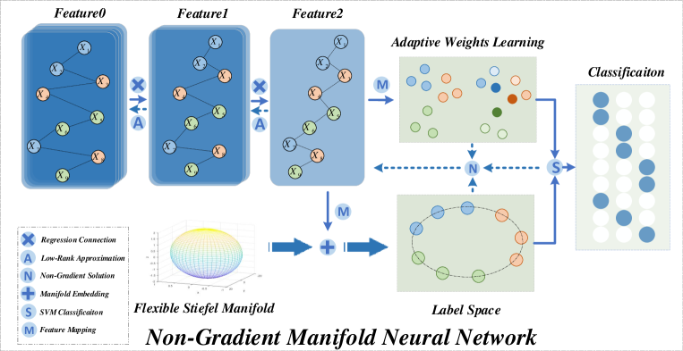
Figure 1: A framework of the proposed model. The blue, orange and green nodes represent three different data. As is shown, the reconstruction regression network extracts the deep features whose distribution satisfies a latent regression. Then, on the one hand, a flexible Stiefel manifold is embedding into the label space. On the other hand, these features are assigned with different weights via adaptive learning. Finally, unifying the two kinds of information, the model predicts the labels via SVM.

From Eq. (3), DNN generally takes thousands of iterations to optimize and obtain the approximate solutions of $\theta$. Besides, the value of the learning rate extremely affects the performance and convergence of the model. For example, if the value of $\alpha$ is improper, the loss will be unstable near the minima and the model can not converge. Therefore, we reconstruct the network via ridge regression to accelerate the convergence. In addition, as shown in Eq. (2), softmax mainly classifies the data according to the value of deep features and the property of the exponential function. However, it is weak to utilize the inner distribution of the data and exists AI ethical problems with low interpretability. Compared with softmax, the SVM aims to find the hyper-planes in label space for classification.

2.2 Multi-Class Support Vector Machine

As a fundamental model of machine learning, Support Vector Machine (SVM) pradhan2012support has been developed mostly in classification and regression. It utilizes the topological information in the label space to find a hyper-plane for binary classification and make the margin maximum. The classic objective function of SVM can be defined as

$$\min\limits_{\bm{w}}\frac{1}{2}\|\bm{w}\|_{2}^{2},\quad s.t.\ y_{i}(\bm{w}^{T}\bm{x}_{i}+b)\geq 1,\ i=1,...,n,$$ (4)

where $\bm{w}$ and $b$ are the parameters to learn, $\bm{x}_{i}\in R^{d}$ is the $i$-th sample, and $y_{i}\in\left\{-1,1\right\}$ is the label of $\bm{x}_{i}$. Furthermore, define the $\xi(\bm{w},b|\bm{x}_{i})$ as the misclassification loss, Eq. (4) can be written as ${\min}_{\bm{w},b}\sum_{i=1}^{n}\xi(\bm{w},b|\bm{x}_{i})+\lambda||w||_{2}^{2}$ where $\lambda$ is the trade-off parameters. Apart from that, the soft margin generally is utilized to avoid the over-fitting and the $\xi(\bm{w},b|\bm{x}_{i})$ represnets the square hinge loss which can be defined as $\xi(\bm{w},b|\bm{x}_{i})=(1-y_{i}(\bm{w}^{T}\bm{x}_{i}+b))_{+}^{2}$. Thus, the primal loss can be given as

$$\min\limits_{\bm{w},b}\sum_{i=1}^{n}(1-y_{i}(\bm{w}^{T}\bm{x}_{i}+b))_{+}^{2}+\lambda||\bm{w}||_{2}^{2}.$$ (5)

The One-versus-Rest (OvR) strategy is employed to extend the binary SVM into multi-class scenarios. Besides, all classifiers can be simultaneously optimized like Crammer2002On . Therefore, the multi-class formulation of Eq. (5) can be written as

$$\min\limits_{\bm{w}_{j},b_{j}}\sum_{j=1}^{c}\sum_{i=1}^{n}[(\bm{w}_{j}^{T}\bm{x}_{i}+b_{j})-y_{ij}-y_{ij}m_{ij}]^{2}+\lambda||\bm{w}_{j}||_{2}^{2},$$ (6)

where $c$ is the number of classes and $y_{ij}$ is the element of the one-hot label matrix $\bm{Y}\in R^{c\times n}$. $m_{ij}$ is the element of slack matrix $\bm{M}\in R^{c\times n}$. Apart from that, 2012Multi introduces the $l_{2,1}$-norm to avoid the model misled by the outliers. Aiming to improve the performance, the scaling factor is integrated with SVM for feature selection 2017Feature . Although the method mentioned above has improved the performance of the SVM, they ignore the latent distribution of the data. In this paper, we not only unify the flexible Stiefel manifold with adaptive SVM to fit the inner manifold structure of the deep embeddings but also employ it as a novel decision layer with higher interpretability for a manifold neural network.

3 Non-Gradient Manifold Neural Network

Aiming to tackle the weakness referred to in Subsection 2.1, we propose a novel manifold neural network. The network is reconstructed via ridge regression and low rank approximation. Apart from that, it embeds a flexible Stiefel manifold into an adaptive support vector machine to act as a decision layer. More importantly, a novel backward optimization with non-gradient is designed to solve the model and obtain the closed-form results directly. The framework is illustrated in Fig 1. Besides, the proof of all lemmas and theorems is listed in supplementary.

3.1 Reconstruct Network via Ridge Regression

Aiming to accelerate the convergence and obtain the closed-form results, we reconstruct the neural network. The forward propagation Eq. (1) can be reformulated as

$$\bm{H}^{l}=\sigma((\bm{W}^{l})^{T}\bm{H}^{l-1}+\bm{b}^{l}\bm{1}_{n}^{T})\Leftrightarrow\min\limits_{\bm{H}^{l}}||\bm{H}^{l}-\sigma((\bm{W}^{l})^{T}\bm{H}^{l-1}+\bm{b}^{l}\bm{1}_{n}^{T})||_{F}^{2},$$ (7)

where the left part can be obtained by taking the derivation of the right equation w.r.t $\bm{H}^{l}$.

Assumption: Noticing that the activation function is generally invertible, we can define the invertibility of the activation function as $\sigma^{-1}(\cdot)$.

Forward ridge regression: From Eq. (7), this forward propagation tries to embed more original and real data information in the deep reconstruction features. Moreover, based on the above assumption, we can make some relaxation and the backward optimization of each layer can be defined as

$$\min\limits_{\bm{W}^{l},\bm{b}^{l}}||(\bm{W}^{l})^{T}\bm{H}^{l-1}+\bm{b}^{l}\bm{1}_{n}^{T}-\sigma^{-1}(\bm{H}^{l})||_{F}^{2}.$$ (8)

Aiming to work out overfitting and has excellent performance on a small dataset, we introduce the $F$-norm regularization for the designed network:

$$\min\limits_{\bm{W}^{l},\bm{b}^{l}}||(\bm{W}^{l})^{T}\bm{H}^{l-1}+\bm{b}^{l}\bm{1}_{n}^{T}-\sigma^{-1}(\bm{H}^{l})||_{F}^{2}+\lambda||\bm{W}^{l}||_{F}^{2},$$ (9)

where $\lambda$ is the trade-off of the regularization term. The $\bm{b}^{l}$ can be solved by Lemma 1.

Lemma 1.

Given a feature matrix $\bm{X}$ and a label matrix $\bm{Y}$, the problem $\min\limits_{\bm{b}}||\bm{W}^{T}\bm{X}+\bm{b}\bm{1}_{n}^{T}-\bm{Y}||_{F}^{2}+\lambda||\bm{W}||_{F}^{2}$ can be solved by $\bm{b}=\frac{\bm{Y}-\bm{W}^{T}\bm{X}}{n}\bm{1}_{n}$.

Having solved the $\bm{b}$, we replace it into the Eq. (9) like

$$\begin{split}\min\limits_{\bm{W}^{l}}&||\bm{W}^{T}\bm{X}+\frac{\sigma^{-1}(\bm{H}^{l})-\bm{W}^{T}\bm{X}}{n}\bm{1}_{n}\bm{1}_{n}^{T}-\sigma^{-1}(\bm{H}^{l})||_{F}^{2}+\lambda||\bm{W}^{l}||_{F}^{2}\\ =\min\limits_{\bm{W}^{l}}&||\bm{W}^{T}\bm{X}\bm{C}-\sigma^{-1}(\bm{H}^{l})\bm{C}||_{F}^{2}+\lambda||\bm{W}^{l}||_{F}^{2},\\ \end{split}$$ (10)

where $\bm{C}=\bm{I}_{n}-\frac{1}{n}\bm{1}_{n}\bm{1}_{n}^{T}$ and $\bm{I}_{n}\in R^{n\times n}$ is a identity matrix. $\bm{C}\in R^{n\times n}$ is a centralized matrix according to the column. To represent more conveniently, we define the matrix $\hat{\bm{Y}}^{l}=\sigma^{-1}(\bm{H}^{l})$ and the problem Eq. (10) can be transformed into

$$\min\limits_{\bm{W}^{l}}||(\bm{W}^{l})^{T}\bm{X}_{\bm{C}}^{l}-\bm{\hat{Y}}_{\bm{C}}^{l}||_{F}^{2}+\lambda||\bm{W}^{l}||_{F}^{2},$$ (11)

where $\bm{X}_{\bm{C}}^{l}=\bm{X}^{l}\bm{C}$ and $\bm{\hat{Y}}_{\bm{C}}^{l}=\bm{\hat{Y}}^{l}\bm{C}$. Problem (11) can be solved by Lemma 2.

Lemma 2.

Given a feature matrix $\bm{X}$ and a label matrix $\bm{Y}$, the problem $\min\limits_{\bm{W}}||\bm{W}^{T}\bm{X}-\bm{Y}||_{F}^{2}+\lambda||\bm{W}||_{F}^{2}$ can be solved by $\bm{W}=(\bm{X}\bm{X}^{T}+\lambda\bm{I}_{d})^{-1}\bm{X}\bm{Y}^{T}$.

By stacking the novel layer Eq. (7), the model successfully extracts the deep feature embedded with the original data information via ridge regression. Moreover, Lemma 1 and Lemma 2 are utilized to obtain the analytic solution of the parameters without gradient.

Low rank backward approximation: Aiming to propagate the label information from the output layer to the input layer, the low rank reconstruction is employed during the backward optimization. Taking the $l$-th layer as an example, the problem can be reformulated as

$$\min\limits_{\bm{H}^{l-1}}||(\bm{W}^{l})^{T}\bm{H}^{l-1}+\bm{b}^{l}\bm{1}_{n}^{T}-\tilde{\bm{Y}}^{l}||_{F}^{2},$$ (12)

where $\tilde{\bm{Y}}^{l}$ is the label matrix in $l$-th layer. Since the analytical results of parameters can be directly obtained via the above lemmas, Eq. (12) is equal to

$$\bm{W}^{l}(\bm{W}^{l})^{T}\bm{H}^{l-1}=\bm{W}^{l}(\tilde{\bm{Y}}^{l}-\bm{b}^{l}\bm{1}_{n}^{T}).$$ (13)

The left of Eq. (13) shows that the input feature firstly is mapped into a $c$-dimensional low rank subspace and reconstructed into a $d$-dimensional space. This procedure can be viewed as

$$\min\limits_{rank(\bm{\bar{}}{\bm{H}})\leq c}||\bm{H}^{l-1}-{\bar{\bm{H}}}||_{F}^{2}=\min\limits_{\bm{V},\bm{W}^{T}\bm{W}=\bm{I}_{c}}||\bm{H}^{l-1}-\bm{W}\bm{V}^{T}||_{F}^{2},$$ (14)

where $\bar{\bm{H}}$ is the reconstructed matrix of the input feature. $\bm{W}\in R^{d\times c}$ is employed as a base vector matrix and $\bar{\bm{H}}$ can be decomposed as $\bar{\bm{H}}=\bm{W}\bm{V}^{T}$. Then, the matrix $\bm{V}$ is easily solved via taking the derivative of Eq. (14) w.r.t $\bm{V}$ and setting it to 0. The result is like $\bm{V}=\bm{X}^{T}\bm{W}$. Therefore, $\bm{H}^{l-1}$ is an approximate solution of $\bm{W}^{l}{\bm{W}^{l}}^{T}\bm{H}^{l-1}$ based on low rank reconstruction and the label backward can be defined like

$$\bar{\bm{H}}^{l-1}=\bm{W}^{l}(\tilde{\bm{Y}}^{l}-\bm{b}^{l}\bm{1}_{n}^{T}).$$ (15)

In order to promote the stability of the model, Softmax is introduced to map the reconstructed label matrix $\tilde{\bm{Y}}^{l-1}=\bar{\bm{H}}^{l-1}$ into $(0,1)$. The whole network works as Algorithm 1.

Algorithm 1 Reconstruct Neural Network via Ridge Regression

0:  data matrix $\bm{X}$, (i.e., $\bm{H}^{0}$), one-hot label matrix $\bm{Y}$.

1:  Initialize $\bm{W}^{l}$ and $\bm{b}^{l}$ of each layer;

2:  while $not\;Convergence$ do

3:     Forward inference via Eq. (7);

4:     for $l=t$ to $1$ do

5:        Optimize the loss Eq. (9) of $l$-th layer via Lemma 1 and Lemma 2;

6:        Propagate the label information to the $l$-$1$-th layer via Eq. (15);

7:     end for

8:  end while

3.2 Decision Layer with Flexible Stiefel Manifold

Although softmax can predict the label according to the value of features and has been widely utilized as a decision layer for classification, it ignores the latent distribution of the data and is weak in interpretation. As is known to us, the support vector machine (SVM) utilizes the distribution of data in label space to find the optimal hyper-planes whose marges generated from the support vector are maximum. Therefore, the multi-class SVM is employed as the decision layer for classification. Inspired by 9390382 , Eq. (6) can be reformulated as

$$\min\limits_{\bm{W},\bm{b},\bm{M}\geq 0}\sum\limits_{i=1}^{n}\underbrace{||\bm{W}^{T}\bm{x}_{i}+\bm{b}-\bm{y}_{i}-\bm{y}_{i}\odot\bm{m}_{i}||_{2}^{2}}_{f_{i}}+\lambda\|\bm{W}\|_{F}^{2},$$ (16)

where $\bm{M}=[\bm{m}_{1},\bm{m}_{2},...,\bm{m}_{n}]\in R^{c\times n}$ is a slack variable to encode the loss of each $\bm{x}_{i}\in R^{d\times 1}$. In the label space, because some nodes may be contaminated by noises or far away from the hyper-lines, these $\bm{f}_{i}$ will be much large, which leads to the model mainly optimize this part of loss and disturbs the performance sharply. Therefore, the adaptive weight vector $\bm{\alpha}\in R^{n\times 1}$ is introduced into the decision layer to enable the model to pay more attention to good nodes for example support vector with $\bm{f}_{i}=0$. It can be formulated as

$$\min\limits_{\bm{\alpha}^{T}\bm{1}_{n}=1,\bm{W},\bm{b},\bm{M}\geq 0}\sum\limits_{i=1}^{n}\alpha_{i}f_{i}+\lambda\|\bm{W}\|_{F}^{2}+\gamma||\bm{\alpha}||_{2}^{2},$$ (17)

where $\gamma$ is a trade-off coefficient and can control the sparsity of $\bm{\alpha}$. We can obtain the closed-form results of this weight vector via Theorem 1.

Theorem 1.

Suppose that $f_{(1)}\leq f_{(2)}\leq...\leq f_{(n)}$. If $\gamma=\frac{n-1}{2}f_{(n)}-\frac{1}{2}\sum_{i=1}^{n-1}f_{(i)}$, the optimal $\bm{\alpha}$ is

$$\alpha_{i}=(\frac{f_{(n)}-f_{(n-1)}}{(n-1)f_{(n)}-\sum\limits_{j=1}^{k}f_{(j)}})_{+}.$$ (18)

Inspired by the successful application of manifold learning in representation learning, we employ the flexible Stiefel Manifold 9134971 formulated in Definition 1 to explore the inner distribution of the data.

Definition 1.

(Flexible Stiefel Manifold) For a matrix $\bm{A}\in R^{a\times b}$, $\bm{A}$ obeys flexible Stiefel manifold if $\bm{A}\in\left\{\bm{B}\in R^{a\times b}|\bm{B}\bm{D}\bm{B}^{T}+\bm{E}=\bm{I}_{a},\bm{D}\geq 0\right\}$, where $\bm{E}$ is a residual matrix.

According to this definition, we assume that the predicted label vectors exist in a flexible Stiefel manifold space. To keep the discussion convenient, we introduce the weighted-centralized matrix $\hat{\bm{C}}=\bm{I}_{n}-\frac{1}{\bm{1}_{n}^{T}\bm{D}\bm{1}_{n}}\bm{D}\bm{1}_{n}\bm{1}_{n}^{T}$ and $\bm{D}={\rm diag}(\bm{\alpha})$. Therefore, the label manifold space can be defined as

$$\bm{W}^{T}\bm{X}\hat{\bm{C}}\bm{D}\hat{\bm{C}}^{T}\bm{X}^{T}\bm{W}+\bm{E}=\bm{I}_{c}.$$ (19)

Owing to $\bm{E}$, this flexible manifold can fit plenty of latent irregular manifold structures. Generally, the error matrix is assumed to satisfy $\bm{E}=\hat{\lambda}\bm{W}^{T}\bm{W}$. Then, the energy can be defined with $\|\bm{E}\|=\hat{\lambda}tr(\bm{W}^{T}\bm{W})=\hat{\lambda}\|\bm{W}\|_{F}^{2}$. To avoid introducing new parameters, we utilize the $\lambda$ to substitute for $\lambda+\hat{\lambda}$ with a hyper-parameter trick. Therefore, the problem can be reformulated as

$$\begin{split}&\min\limits_{\bm{\alpha},\bm{M},\bm{W},\bm{b}}\sum\limits_{i=1}^{n}\alpha_{i}||(\bm{W}^{t})^{T}\bm{h}_{i}^{t-1}+\bm{b}-\bm{y}_{i}-\bm{y}_{i}\odot\bm{m}_{i}||_{2}^{2}+\lambda\|\bm{W}\|_{F}^{2}+\gamma||\bm{\alpha}||_{2}^{2}\\ &~{}~{}~{}~{}~{}~{}~{}~{}s.t.\ \bm{W}^{T}(\bm{X}\hat{\bm{C}}\bm{D}\hat{\bm{C}}^{T}\bm{X}^{T}+\lambda\bm{I}_{d})\bm{W}=\bm{I}_{c},\bm{\alpha}^{T}\bm{1}_{n}=1,\bm{\alpha}\geq 0,\bm{M}\geq 0.\end{split}$$ (20)

By embedded the flexible manifold, Eq. (20) successfully utilizes the inner distribution of the data for classification. The following Theorem 2 can provide the closed-form results for this problem.

Theorem 2.

Suppose that $\bm{\alpha}$ is a constant and let $\bm{G}=\bm{Y}-\bm{Y}\odot\bm{M}$. $\bm{W}$ and $\bm{b}$ can be solved by

$$\bm{W}=\bm{S}^{-1}\bm{U}\bm{\Lambda}^{T}\bm{V}^{T}\quad and\quad\bm{b}=\frac{\bm{G}\bm{D}\bm{1}_{n}-\bm{W}^{T}\bm{X}\bm{D}\bm{1}_{n}}{\bm{1}_{n}^{T}\bm{D}\bm{1}_{n}}$$ (21)

where $\bm{S}=(\bm{X}\hat{\bm{D}}\bm{X}^{T}+\lambda\bm{I}_{d})^{\frac{1}{2}}$, $\hat{\bm{D}}=\hat{\bm{C}}\bm{D}\hat{\bm{C}}^{T}$ and $\bm{\Lambda}=[\bm{I}_{c},\bm{0}]\in R^{c\times d}$. $\bm{U},\bm{V}$ are the left and right singular of $\bm{S}^{-1}\bm{X}\hat{\bm{D}}\bm{G}$, respectively. Having obtained the solution of $\bm{W},\bm{b}$, slack variable $\bm{M}$ can be solved by

$$\bm{m}_{i}=(\bm{y}_{i}\odot(\bm{W}^{T}\bm{x}_{i}+\bm{b})-\bm{1}_{c})_{+}.$$ (22)

Algorithm 2 Manifold Neural Network

0:  data matrix $\bm{X}$, (i.e., $\bm{H}^{0}$), one-hot label matrix $\bm{Y}$, trade-pff parameters $\lambda$ and $\gamma$.

1:  Initialize $\bm{W}^{l}$ and $\bm{b}^{l}$ of each layer;

2:  while $not\;Convergence$ do

3:     Forward inference via Eq. (23);

4:     Optimize the $\bm{\alpha}$, $\bm{M}$, $\bm{W}^{t}$ and $\bm{b}^{t}$ via Theorem 1 and Theorem 2;

5:     for $l=L-1$ to $1$ do

6:        Optimize the loss Eq. (9) of $l$-th layer via Lemma 1 and Lemma 2;

7:        Propagate the label information to the $l-1$-th layer via Eq. (15);

8:     end for

9:  end while

3.3 A Novel Manifold Neural Network

Although Eq. (20) not only has strong interpretability but also explores the latent distribution of the data with flexible Stiefel manifold, it can not has good performance when facing non-linear problems. Aiming to solve this problem, we use the reconstructed neural network proposed in Eq. (7) to extract the feature and employ Eq. (20) to learn the latent manifold of the embedding for classification. Then, we finally put forward a novel manifold neural network like

$$\left\{\begin{array}[]{l}\begin{split}&\min\limits_{\bm{H}^{l}}||\bm{H}^{l}-\sigma((\bm{W}^{l})^{T}\bm{H}^{l-1}+\bm{b}^{l}\bm{1}_{n}^{T})||_{F}^{2}\\ &\min\limits_{\mathcal{F}}\sum\limits_{i=1}^{n}\alpha_{i}{||(\bm{W}^{t})^{T}\bm{h}_{i}^{t-1}+\bm{b}-\bm{y}_{i}-\bm{y}_{i}\odot\bm{m}_{i}||_{2}^{2}}+\lambda\|\bm{W}^{t}\|_{F}^{2}+\gamma||\bm{\alpha}||_{2}^{2},\\ \end{split}\par\end{array}\right.$$ (23)

where $\mathcal{F}=\left\{\bm{W}^{t},\bm{b}^{t},\bm{\alpha},\bm{M}\right\}$ satisfies the same constraints shown in Eq. (20) , $l\in\left\{0,1,...,t\right\}$ is the $l$-th layer in manifold neural network and $\bm{y}_{i}\in R^{c}$ is the one-hot label of the $i$-th node. Moreover, the whole network is jointly optimized via Algorithm 2.

The Merits of the Proposed Model: Compared with the classic deep neural network, the proposed network obtains closed-form results via ridge regression reconstruction and accelerates convergence. Besides, by embedding the flexible Stiefel manifold into the decision layer, the model successfully learns the distribution of the deep embeddings. Moreover, the multi-class SVM with adaptive weights is unified with the decision layer, which makes the model more explicable. Finally, we propose a novel manifold neural network and design a joint optimization strategy that can directly obtain the closed-form solution of each parameter.

3.4 Time Complexity

Owing to reconstructing the neural network via ridge regression, the computational complexity is $O(n^{2}d_{l})$. For the decision layer, calculating the $\bm{M}$ and $\bm{\alpha}$ need $O(ncd_{t-1})$ and $O(n\log n+n)$. To obtain the $\bm{W}^{t}$, the total time complexity is $O(nd_{t-1}c+d_{t-1}^{2}c+d_{t-1}c^{2}+d_{t-1}^{3})$. Then, update the $\bm{b}^{t}$ takes $O(cn+n+d_{t-1}n+cd_{t-1})$. In sum, the whole model needs $O(T(tn^{2}d_{l}+ncd_{t-1}+n\log n+d_{t-1}^{2}c+d_{t-1}c^{2}))$, where $t$ is the number of the feature extraction layers and $T$ represents the number of iterations. In practice, since $n$ is much larger than $d_{l}$ and $c$, the time complexity can be approximated as $O(Ttn^{2})$.

Table 1: Datasets Description

Dataset	AT&T	UMIST	WAVEFORM	MNIST-Mini	MNIST	FashionMNIST
# of samples	400	575	2746	10000	70000	70000
Features	1024	1024	21	784	784	784
Classes	40	20	3	10	10	10

4 Experiment

In this paper, we propose a novel neural network and a non-gradient optimization strategy. Therefore, the experiment mainly verifies the feasibility and performance of the proposed network based on the completely non-gradient strategies. Therefore, we select six comparison methods including DNN.

Table 2: Accuracy(%) and F1-score(%) on Benchmark Datasets

		AT&T	WAVEFORM	UMIST	MNIST-MINI	MNIST	FashionMNIST
	Acc	8.77$\pm$0.41	56.98$\pm$0.19	20.00$\pm$1.19	23.58$\pm$0.02	23.58$\pm$0.15	36.86$\pm$0.12
RidgeReg	F1	6.94$\pm$0.22	58.11$\pm$0.19	14.98$\pm$2.00	13.81$\pm$1.74	16.99$\pm$0.50	24.69$\pm$0.07
	Acc	5.83$\pm$1.78	57.04$\pm$0.78	21.39$\pm$2.44	23.53$\pm$0.26	23.29$\pm$0.22	36.85$\pm$0.07
LassoReg	F1	4.40$\pm$1.41	58.22$\pm$0.81	14.77$\pm$1.83	17.21$\pm$0.51	17.75$\pm$1.19	25.32$\pm$0.86
	Acc	86.67$\pm$1.93	72.60$\pm$0.53	75.14$\pm$1.83	81.29$\pm$0.22	88.71$\pm$0.12	79.49$\pm$0.25
SmartSVM	F1	87.05$\pm$1.17	72.38$\pm$0.55	72.52$\pm$1.59	81.05$\pm$0.23	88.60$\pm$0.12	79.49$\pm$0.25
	Acc	90.00$\pm$2.93	76.33$\pm$1.23	96.88$\pm$0.62	75.25$\pm$1.67	62.15$\pm$0.11	43.46$\pm$0.17
MKVM	F1	92.92$\pm$2.86	72.24$\pm$1.64	95.84$\pm$0.58	74.47$\pm$1.89	60.95$\pm$0.12	42.18$\pm$0.16
	Acc	51.67$\pm$8.07	67.48$\pm$6.41	89.02$\pm$0.05	75.47$\pm$2.69	55.34$\pm$0.05	50.94$\pm$2.39
SVM	F1	56.59$\pm$8.05	56.59$\pm$10.99	87.33$\pm$0.16	75.56$\pm$2.43	54.80$\pm$0.03	50.59$\pm$3.61
	Acc	50.89$\pm$1.74	83.98$\pm$3.96	72.83$\pm$1.89	75.33$\pm$2.39	81.79$\pm$2.69	80.72$\pm$1.35
DNN	F1	35.94$\pm$0.11	83.69$\pm$4.62	58.73$\pm$0.06	67.05$\pm$0.89	68.44$\pm$0.09	78.09$\pm$1.11
	Acc	98.75$\pm$0.06	85.44$\pm$0.01	97.39$\pm$0.11	84.83$\pm$0.36	83.67$\pm$0.35	79.54$\pm$0.15
Ours	F1	97.94$\pm$0.46	84.12$\pm$0.18	97.09$\pm$0.04	84.95$\pm$0.29	84.60$\pm$0.39	80.14$\pm$0.11

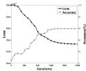
(a) UMIST: DNN

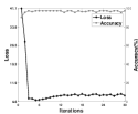
(b) UMIST: OURS

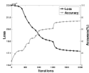
(c) MNIST-Mini: DNN

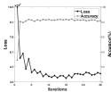
(d) MNIST-Mini: OURS

Figure 2: Relationship between loss, accuracy, and iterations for DNN and proposed network on datasets including UMIST, MNIST-Mini. The four figures show the performance and convergence of methods.

4.1 Dataset Description and Experimental Settings

Six benchmark datasets involved in our experiments are AT&T341300 , WAVEFORM2013UCI , UMIST6565365 , MNIST-MINI, MNIST726791 , and FashionMNISTxiao2017fashionmnist . The detail of these datasets is listed in Table 1. We compare the proposed network with six classic methods including Ridge Regression ($RidgeReg$), Lasso Regression ($LassoReg$), the Hierarchical Multiclass Support Vector Machine ($SmartSVM$) 2017Fast , the Multiclass Kernel-based Vector Machine ($MKVM$) Crammer2002On , SVM with OVR ($SVM$) and Deep Neural Network ($DNN$).

Before classification, all benchmark datasets are accordingly (row-)normalized to the range of $[0,1]$. Mnist and FashionMnist are used $60000$ data as the training data and $10000$ data as the testing data. Except for these two datasets, the other datasets are split into a training dataset ($80\%$) and a testing dataset ($20\%$). Because several methods involve trade-off coefficients, we choose values of these parameters from $\left\{2^{-3},2^{-2},2^{-1},2^{0},2^{1},2^{2},2^{3}\right\}$ and record the best results. The gradient descent is utilized to optimize the DNN. The learning rate is $0.01$ and the iteration is $2000$. The iteration of our model is 30. Apart from that, the proposed model and DNN use the same structure. For AT&T, two layers are used and the hidden units are 64. The other five datasets adopt 3 layers. Among them, the hidden units in WAVEFORM are 10 and 4. The hidden units in UMIST are 64 and 32. For MNIST and FashionMinst, the hidden units are 32 and 16. Accuracy and F1-score are employed to evaluate these different methods.

4.2 Analysis of Experiments

Aiming to evaluate the performance of the proposed model more accurately, the models mentioned above are run 10 times on the datasets. The results including mean value and standard deviation are shown in Table 2. Based on this, we can conclude that

1) The proposed network achieves great performance on all benchmark datasets. It obtains the top accuracy and F1-score of classification on the first four datasets. On the Mnist, it also achieves the second-highest score.

2) When the number of categories is large, ours still has a good ability to predict the label accurately especially on AT&T and UMIST.

3) With the help of a more reasonable and efficient decision layer, the proposed novel network compared with DNN has a better performance.

Furthermore, aiming to study the convergence and performance of the proposed network, we compare the loss and accuracy of DNN and ours with the number of iterations. The results are shown in Fig 2. The proposed network can converge within 5 iterations regardless of the size of the datasets. On the contrary, it is almost necessary to optimize the DNN by more than 1000 iterations to converge. Based on this, we can infer that the designed non-gradient strategy is more efficient than gradient descent. Besides, by embedded the flexible Stiefel manifold and utilized the adaptive weights, the proposed network successfully explores the inner distribution of the data and obtains a higher accuracy.

4.3 Sensitivity Analysis w.r.t. Parameter $\lambda$

In this part, we conduct the corresponding experiments to study the sensitivity of our network Eq. (23) regarding to $\lambda$. The two datasets, AT&T and UMIST, are preprocessed and split according to Subsection 4.1. Besides, $\lambda$ varies from $\left\{2^{-3},2^{-2},2^{-1},2^{0},2^{1},2^{2},2^{3}\right\}$. The accuracy and F1-score related to it are suggested in Fig 3.

$1)$ The curves of two indices are steady when $\lambda$ is relevant small like $\lambda\leq 2^{-1}$. However, the performance of the proposed model drops rapidly when $\lambda$ is larger.

$2)$ Our network is insensitive to trade-off parameter $\lambda$, when $\lambda<2^{0}$. Therefore, we can either fine-tune $\lambda$ in $(0,1]$ or simply set it as a median like $0.5$.

Table 3: Ablation Study on Three Datasets

	AT&T		WAVEFORM		UMIST
	ACC	F1	ACC	F1	ACC	F1
DNN	50.89$\pm$1.74	35.94$\pm$0.11	83.98$\pm$3.96	83.69$\pm$4.62	72.83$\pm$1.89	58.73$\pm$0.06
RidgeR-NN	90.86$\pm$0.03	91.42$\pm$0.02	68.49$\pm$4.11	65.94$\pm$5.23	93.91$\pm$0.47	93.92$\pm$1.19
RidgeR-SVM-NN	94.17$\pm$0.02	95.75$\pm$0.01	84.26$\pm$1.80	83.85$\pm$1.81	97.39$\pm$0.47	97.01$\pm$0.47
RidgeR-SVM-AW-NN	98.75$\pm$0.06	97.94$\pm$0.46	85.44$\pm$0.01	84.12$\pm$0.18	97.39$\pm$0.11	97.09$\pm$0.04

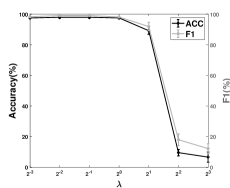
(a) AT&T

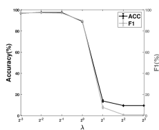
(b) UMIST

Figure 3: Accuracy and F1-score of the proposed network w.r.t the varying parameter $\lambda\in\left\{2^{-3},2^{-2},2^{-1},2^{0},2^{1},2^{2},2^{3}\right\}$.

4.4 Ablation Study

We conduct an ablation study to evaluate how each part of the proposed network including reconstruction strategy with ridge regression (RidgeR), the flexible Stiefel Manifold SVM (SVM), and the adaptive weight (AW), contribute to overall model performances. Besides, the classic DNN with softmax is utilized as a baseline. The results are summarized in Table 3. We confirm that the non-gradient optimization algorithm 1 provides the RidgeR network with the closed-form results, which is helpful to improve the performance. Moreover, contrasted with softmax, SVM assists the model to discover the latent data distribution. Besides, it is shown that unifying the SVM with adaptive weight can make the model more interpretable and further improve performance.

5 Conclusion

In this paper, we propose a novel non-gradient neural network. Compared with the classic deep neural network optimized via gradient descent, it can be solved with closed-form results via the proposed algorithms which have a faster convergent speed. Besides, it unifies the flexible Stiefel manifold and adaptive weights into the SVM acted as the decision layer, which successfully utilizes the inner structure of the data to predict the label and improve the performance significantly. On the benchmark datasets, the proposed network achieves excellent results. In the future, we will attempt to provide the convolutional neural network with a non-gradient optimized strategy.

Appendix A Proof of Lemma 1

Lemma 1.

Given a feature matrix $\bm{X}$ and a label matrix $\bm{Y}$, the problem

$$\min\limits_{\bm{b}}||\bm{W}^{T}\bm{X}+\bm{b}\bm{1}_{n}^{T}-\bm{Y}||_{F}^{2}+\lambda||\bm{W}||_{F}^{2}$$ (24)

can be solved by $\bm{b}=\frac{\bm{Y}-\bm{W}^{T}\bm{X}}{n}\bm{1}_{n}$.

Proof.

Lemma 1 aims to solve the the $\bm{b}$. Therefore, the problem (24) is formulated as

$$\begin{split}\mathcal{J}&=\min\limits_{\bm{b}}||\bm{W}^{T}\bm{X}+\bm{b}\bm{1}_{n}^{T}-\bm{Y}||_{F}^{2}\\ &\Rightarrow\min\limits_{\bm{b}}{\rm Tr}((\bm{W}^{T}\bm{X}+\bm{b}\bm{1}_{n}^{T}-\bm{Y})^{T}(\bm{W}^{T}\bm{X}+\bm{b}\bm{1}_{n}^{T}-\bm{Y}))\\ &\Rightarrow\min\limits_{\bm{b}}2{\rm Tr}(\bm{1}_{n}\bm{b}^{T}\bm{W}^{T}\bm{X})+{\rm Tr}(\bm{1}_{n}\bm{b}^{T}\bm{b}\bm{1}_{n}^{T})+2{\rm Tr}(\bm{1}_{n}\bm{b}^{T}\bm{Y}).\end{split}$$ (25)

Owing to constraint on $\bm{b}$, Eq. (25) is derivated w.r.t $\bm{b}$ and set to $0$ like

$$\left\{\begin{split}\nabla_{\bm{b}}\mathcal{J}&=0\\ \bm{b}\bm{1}_{n}^{T}\bm{1}_{n}&=\bm{Y}\bm{1}_{n}-\bm{W}^{T}\bm{X}\bm{1}_{n}.\\ \end{split}\right.$$ (26)

Then, we have $\bm{b}=\frac{\bm{Y}-\bm{W}^{T}\bm{X}}{n}\bm{1}_{n}$. ∎

Appendix B Proof of Lemma 2

Lemma 2.

Given a feature matrix $\bm{X}$ and a label matrix $\bm{Y}$, the problem

$$\min\limits_{\bm{W}}||\bm{W}^{T}\bm{X}-\bm{Y}||_{F}^{2}+\lambda||\bm{W}||_{F}^{2}$$ (27)

can be solved by $\bm{W}=(\bm{X}\bm{X}^{T}+\lambda\bm{I}_{d})^{-1}\bm{X}\bm{Y}^{T}$.

Proof.

Lemma 2 aims to solve the the $\bm{W}$. Therefore, the problem (27) is formulated as

$$\begin{split}\mathcal{L}&=\min\limits_{\bm{W}}||\bm{W}^{T}\bm{X}-\bm{Y}||_{F}^{2}+\lambda||\bm{W}||_{F}^{2}\\ &\Rightarrow\min\limits_{\bm{W}}{\rm Tr}((\bm{W}^{T}\bm{X}-\bm{Y})^{T}(\bm{W}^{T}\bm{X}-\bm{Y}))+\lambda{\rm Tr}(\bm{W}^{T}\bm{W})\\ &\Rightarrow\min\limits_{\bm{W}}{\rm Tr}(\bm{X}^{T}\bm{W}\bm{W}^{T}\bm{X})-2{\rm Tr}(\bm{W}^{T}\bm{X}\bm{Y}^{T})+\lambda{\rm Tr}(\bm{W}^{T}\bm{W}).\end{split}$$ (28)

Then, Eq. (28) can be solved via taking the derivation of $\bm{W}$ like

$$\left\{\begin{split}\nabla_{\bm{W}}\mathcal{L}&=0\\ (\bm{X}\bm{Y}^{T}+\lambda\bm{I}_{d})\bm{W}&=\bm{X}\bm{Y}^{T}.\\ \end{split}\right.$$ (29)

Due to that $\bm{X}\bm{Y}^{T}+\lambda\bm{I}_{d}$ is a full rank matrix, we can obtain the $\bm{W}=(\bm{X}\bm{X}^{T}+\lambda\bm{I}_{d})^{-1}\bm{X}\bm{Y}^{T}$. ∎

Appendix C Proof of Theorem 1

Theorem 1.

Suppose that $f_{(1)}\leq f_{(2)}\leq...\leq f_{(n)}$. If $\gamma=\frac{n-1}{2}f_{(n)}-\frac{1}{2}\sum_{i=1}^{n-1}f_{(i)}$, the optimal $\bm{\alpha}$ is

$$\alpha_{i}=(\frac{f_{(n)}-f_{(n-1)}}{(n-1)f_{(n)}-\sum\limits_{j=1}^{k}f_{(j)}})_{+}.$$ (30)

Proof.

Theorem 1 aims to solve the $\bm{\alpha}$. Therefore, we fix $M$, $W$ and $\bm{b}$. The objective function is formulated as

$$\min\limits_{\textbf{1}_{n}^{T}\bm{\alpha}=1,\bm{\alpha}\geq 0}\sum\limits_{i=1}^{n}\alpha_{i}f_{i}+\gamma\alpha_{i}^{2},$$ (31)

where $f_{i}=\|W^{T}\bm{x}_{i}+\bm{b}-\bm{y}_{i}-\bm{y}_{i}\odot\bm{m}_{i}\|_{2}^{2}$, $\gamma$ is the trade-off coefficient, and $\bm{\alpha}\in R^{d}$ is the weight vector. The first term in problem.(31) means that a points with large classification errors should be assigned with a small weight. In general, $f_{i}$ can be viewed as a constant value and Eq. (31) has the same solutions with following problem

$$\min\limits_{\textbf{1}_{n}^{T}\bm{\alpha}=1,\bm{\alpha}\geq 0}\|\bm{\alpha}+\frac{\bm{f}}{2\gamma}\|_{2}^{2},$$ (32)

where $\bm{f}=[f_{1},f_{2},...,f_{n}]$. Transformed with the Lagrangian function, the current problem is represented as

$$\mathcal{L}_{\alpha}=\|\bm{\alpha}+\frac{\bm{f}}{2\gamma}\|_{2}^{2}+\xi(1-\sum\limits_{i=1}^{n}\alpha_{i})-\sum\limits_{i=1}^{n}\beta_{i}\alpha_{i},$$ (33)

where $\xi$ and $\beta_{i}$ are the Largranian multipliers. The KKT conditions are given as

$$\left\{\begin{array}[]{l}\frac{\partial\mathcal{L}_{\alpha}}{\partial\alpha_{i}}=\alpha_{i}+\frac{f_{i}}{2\gamma}-\xi-\beta_{i}=0\\ \beta_{i}\alpha_{i}=0\\ \sum\limits_{i=1}^{n}\alpha_{i}=1,\beta_{i}\geq 0,\alpha_{i}\geq 0\end{array}.\right.$$ (34)

Consider the following cases

$$\left\{\begin{array}[]{l}\alpha_{i}=0\Rightarrow\xi-\frac{f_{i}}{2\gamma}=-\beta_{i}\leq 0\\ \alpha_{i}\geq 0\Rightarrow\alpha_{i}=\xi-\frac{f_{i}}{2\gamma}\end{array},\right.$$ (35)

which means

$$\alpha_{i}=(\xi-\frac{f_{i}}{2\gamma})_{+}.$$ (36)

Without loss of generality, we suppose that $f_{(1)}\leq f_{(2)}\leq...\leq f_{(n)}$ and $\alpha_{1}\geq\alpha_{2}\geq\cdots\geq\alpha_{n}$. Therefore, we have

$$\left\{\begin{array}[]{l}\alpha_{k}\textgreater 0\Rightarrow\xi-\frac{f_{(k)}}{2\gamma}>0\\ \alpha_{k+1}=0\Rightarrow\xi-\frac{f_{(k+1)}}{2\gamma}\leq 0\end{array},\right.$$ (37)

where $k\in[1,n]$. Due to $\sum\limits_{i=1}^{n}\alpha_{i}=1$, we have

$$\sum\limits_{i=1}^{n}\alpha_{i}=k\xi-\sum\limits_{i=1}^{k}\frac{f_{(i)}}{2\gamma}=1,$$ (38)

which means

$$\xi=\frac{1}{2k\gamma}\sum\limits_{i=1}^{k}f_{(i)}+\frac{1}{k}.$$ (39)

Combine with our assumption and we have

$$\begin{array}[]{l}\frac{1}{2k\gamma}\sum\limits_{i=1}^{k}f_{(i)}+\frac{1}{k}-\frac{f_{(k+1)}}{2\gamma}\leq 0<\frac{1}{2k\gamma}\sum\limits_{i=1}^{k}f_{(i)}+\frac{1}{k}-\frac{f_{(k)}}{2\gamma}\\ \Rightarrow\frac{f_{(k)}}{2\gamma}<\frac{1}{2k\gamma}\sum\limits_{i=1}^{k}f_{(i)}+\frac{1}{k}\leq\frac{f_{(k+1)}}{2\gamma}\\ \Rightarrow\frac{kf_{(k)}}{2}-\frac{1}{2}\sum\limits_{i=1}^{k}f_{(i)}<\gamma\leq\frac{kf_{(k+1)}}{2}-\frac{1}{2}\sum\limits_{i=1}^{k}f_{(i)}.\end{array}$$ (40)

When $k=n-1$ and $\gamma=\frac{n-1}{2}f_{(n)}-\frac{1}{2}\sum_{i=1}^{n-1}f_{(i)}$, we obtain

$$\begin{split}\alpha_{i}&=(\frac{\sum\limits_{i=1}^{n-1}f_{(i)}+2\gamma}{2(n-1)\gamma}-\frac{f_{(i)}}{2\gamma})_{+}=(\frac{f_{(n)}-f_{(n-1)}}{(n-1)f_{(n)}-\sum\limits_{i=1}^{n-1}f_{(i)}})_{+}\end{split}.$$ (41)

∎

Appendix D Proof of Theorem 2

Theorem 2.

Suppose that $\bm{\alpha}$ is a constant and let $\bm{G}=\bm{Y}-\bm{Y}\odot\bm{M}$. $\bm{W}$ and $\bm{b}$ can be solved by

$$\bm{W}=\bm{S}^{-1}\bm{U}\bm{\Lambda}^{T}\bm{V}^{T}\quad and\quad\bm{b}=\frac{\bm{G}\bm{D}\bm{1}_{n}-\bm{W}^{T}\bm{X}\bm{D}\bm{1}_{n}}{\bm{1}_{n}^{T}\bm{D}\bm{1}_{n}}$$ (42)

where $\bm{S}=(\bm{X}\hat{\bm{D}}\bm{X}^{T}+\lambda\bm{I}_{d})^{\frac{1}{2}}$, $\hat{\bm{D}}=\hat{\bm{C}}\bm{D}\hat{\bm{C}}^{T}$, $\bm{D}={\rm diag}(\bm{\alpha})$ and $\bm{\Lambda}=[\bm{I}_{c},\bm{0}]\in R^{c\times d}$. $\bm{U},\bm{V}$ are the left and right singular of $\bm{S}^{-1}\bm{X}\hat{\bm{D}}\bm{G}$, respectively. Having obtained the solution of $\bm{W},\bm{b}$, slack variable $\bm{M}$ can be solved by

$$\bm{m}_{i}=(\bm{y}_{i}\odot(\bm{W}^{T}\bm{x}_{i}+\bm{b})-\bm{1}_{c})_{+}.$$ (43)

Proof.

Theorem 2 aims to obtain the analytic solutions of $\bm{M}$, $\bm{W}$ and $\bm{b}$. Therefore, the objective function is formulated as

$$\min\limits_{\bm{M}\geq 0,\bm{W},\bm{b}}\sum\limits_{i=1}^{n}\alpha_{i}f_{i}+\lambda\|\bm{W}\|_{F}^{2},\ s.t.\ \bm{W}^{T}(\bm{X}\hat{\bm{C}}\bm{D}\hat{\bm{C}}^{T}\bm{X}^{T}+\lambda\bm{I}_{d})\bm{W}=\bm{I}_{c},\\$$ (44)

where $f_{i}=\|W^{T}\bm{x}_{i}+\bm{b}-\bm{y}_{i}-\bm{y}_{i}\odot\bm{m}_{i}\|_{2}^{2}$. These variables can be divided into two parts, solving slack variable $\bm{M}$ and optimizing parameters, $\bm{W}$ and $\bm{b}$.

$A.\;Optimize\;\bm{M}\;with\;fixing\;\bm{W}\;and\;\bm{b}$

Regarding $\bm{W}$, $\bm{b}$ and $\bm{\alpha}$ as constants, Eq. (44) to optimize the $\bm{M}$ is formulated as the following sub-problems

$$\begin{split}\min\limits_{\bm{m}_{i}\geq 0}\|W^{T}\bm{x}_{i}+b-\bm{y}_{i}-\bm{y}_{i}\odot\bm{m}_{i}\|_{2}^{2}.\end{split}$$ (45)

Due to $\bm{y}_{i}\odot\bm{y}_{i}=1$, Eq. (45) is defined like

$$\min\limits_{\bm{m}_{i}\geq 0}\|\bm{y}_{i}\odot(W^{T}\bm{x}_{i}+b)-\textbf{1}_{c}-\bm{m}_{i}\|_{2}^{2}.$$ (46)

We utilize the Lagrange multipliers to transform Eq. (46) like

$$\mathcal{L}_{m}=\|\bm{y}_{i}\odot(W^{T}\bm{x}_{i}+\bm{b})-\textbf{1}_{c}-\bm{m}_{i}\|_{2}^{2}-\bm{\rho}_{i}^{T}\bm{m}_{i},$$ (47)

where $\bm{\rho}_{i}\geq 0$ is a Lagrange multiplier. Based on KKT conditions, we have the following derivation

$$\left\{\begin{array}[]{l}2\bm{m}_{i}-2\bm{y}_{i}\odot(W^{T}\bm{x}_{i}+\bm{b})+2-\bm{\rho}_{i}=0\\ \bm{\rho}_{i}\odot\bm{m}_{i}=0\\ \bm{\rho}_{i}\geq 0,\bm{m}_{i}\geq 0\end{array}\right..$$

For $m_{ij}=0$, $y_{ij}(W^{T}\bm{x}_{i}+\bm{b})_{j}-1=-\frac{\rho_{ij}}{2}$. Due to $\bm{\rho}_{i}\geq 0$, $-\frac{\rho_{ij}}{2}$ is less than or equal to 0. If $m_{ij}\geq 0$, we can obtain that $m_{ij}=y_{ij}(W^{T}\bm{x}_{i}+\bm{b})_{j}-1$. Therefore, the solution to $\bm{m}_{i}$ is unified as

$$\bm{m}_{i}=(\bm{y}_{i}\odot(W^{T}\bm{x}_{i}+\bm{b})-\textbf{1}_{c})_{+}.$$ (48)

$B.\;Optimize\;\bm{W}\;and\;\bm{b}\;with\;fixing\;\bm{M}$

Having obtained the $\bm{M}$, the objective function can be reformulated as

$$\mathcal{J}=\min\limits_{\bm{W},\bm{b}}\sum\limits_{i=1}^{n}\alpha_{i}||W^{T}\bm{x}_{i}+\bm{b}-\bm{g}_{i}||_{F}^{2}+\lambda\|\bm{W}\|_{F}^{2},\ s.t.\ \bm{W}^{T}(\bm{X}\hat{\bm{C}}\bm{D}\hat{\bm{C}}^{T}\bm{X}^{T}+\lambda\bm{I}_{d})\bm{W}=\bm{I}_{c},\\$$ (49)

where $\bm{G}=\bm{Y}-\bm{Y}\odot\bm{M}$. Since there is no constraint on $\bm{b}$, it can be solved via $\frac{\partial\mathcal{J}}{\partial\bm{b}}=0$ and the closed-form results like

$$\bm{b}=\frac{\bm{G}\bm{D}\bm{1}_{n}-\bm{W}^{T}\bm{X}\bm{D}\bm{1}_{n}}{\bm{1}_{n}^{T}\bm{D}\bm{1}_{n}}.$$ (50)

Therefore, the bias term is rewritten as

$$\bm{b}\bm{1}_{n}^{T}=\bm{G}\frac{1}{\bm{1}_{n}^{T}\bm{D}\bm{1}_{n}}\bm{D}\bm{1}_{n}\bm{1}_{n}^{T}-\bm{W}^{T}\bm{X}\frac{1}{\bm{1}_{n}^{T}\bm{D}\bm{1}_{n}}\bm{D}\bm{1}_{n}\bm{1}_{n}^{T}=(\bm{G}-\bm{W}^{T}\bm{X})(\bm{I}_{n}-\hat{\bm{C}}).$$ (51)

Furthermore, the residual error can be reformulated as

$$\bm{W}^{T}\bm{X}+\bm{b}\bm{1}_{n}^{T}-\bm{G}=(\bm{W}^{T}\bm{X}-\bm{G})-(\bm{W}^{T}\bm{X}-\bm{G})(\bm{I}_{n}-\hat{\bm{C}})=(\bm{W}^{T}\bm{X}-\bm{G})\hat{\bm{C}}.$$ (52)

For simplicity, define $\hat{\bm{D}}=\hat{\bm{C}}\bm{D}\hat{\bm{C}}^{T}$. The problem Eq. (49) can be reformulated as

$$\begin{split}\mathcal{J}&=\min\limits_{\bm{W}}{\rm Tr}((\bm{W}^{T}\bm{X}+\bm{b}\bm{1}_{n}^{T}-\bm{G})^{T}\bm{D}(\bm{W}^{T}\bm{X}+\bm{b}\bm{1}_{n}^{T}-\bm{G}))+\lambda{\rm Tr}(\bm{W}^{T}\bm{W})\\ &\Rightarrow\min\limits_{\bm{W}}{\rm Tr}(((\bm{W}^{T}\bm{X}-\bm{G})\hat{\bm{C}})^{T}\bm{D}((\bm{W}^{T}\bm{X}-\bm{G})\hat{\bm{C}})+\lambda{\rm Tr}(\bm{W}^{T}\bm{W})\\ &\Rightarrow\min\limits_{\bm{W}}{\rm Tr}((\bm{W}^{T}\bm{X}-\bm{G})\hat{\bm{D}}(\bm{W}^{T}\bm{X}-\bm{G})^{T})+\lambda{\rm Tr}(\bm{W}^{T}\bm{W})\\ &\Rightarrow\min\limits_{\bm{W}}{\rm Tr}(\bm{W}^{T}(\bm{X}\hat{\bm{D}}\bm{X}^{T}+\lambda\bm{I}_{d})\bm{W})-2{\rm Tr}(\bm{W}^{T}\bm{X}\hat{\bm{D}}\bm{G}^{T}).\end{split}$$ (53)

Due to that $\bm{W}$ obeys the flexible Stiefel manifold. Therefore, Eq. (53) can be simplified as

$$\mathcal{J}=\max_{\bm{W}^{T}\bm{S}^{2}\bm{W}=I}{\rm Tr}(\bm{W}^{T}\bm{X}\hat{\bm{D}}\bm{G}^{T})\Leftrightarrow\mathcal{J}=\max_{\bm{Q}^{T}\bm{Q}=I}{\rm Tr}(\bm{Q}^{T}\bm{S}^{-1}\bm{X}\hat{\bm{D}}\bm{G}^{T}),$$ (54)

where $\bm{S}=(\bm{X}\hat{\bm{D}}\bm{X}^{T}+\lambda\bm{I}_{d})^{\frac{1}{2}}$ and $\bm{Q}=\bm{S}\bm{W}$. According to Lemma 3, Eq. (54) has the analytic solution like

$$\bm{W}=\bm{S}^{-1}\bm{U}\bm{\Lambda}^{T}\bm{V}^{T},$$ (55)

where $[\bm{U},\sim,\bm{V}]={\rm svd}(\bm{S}^{-1}\bm{X}\hat{\bm{D}}\bm{G}^{T})$ and $\bm{\Lambda}=[\bm{I}_{c},\bm{0}]$.

Lemma 3.

For $\bm{Q},\bm{P}\in R^{m\times n}$ where $m>n$, the problem $\max_{\bm{Q}^{T}\bm{Q}=I}\bm{Q}^{T}\bm{P}$ has the closed-form results like $\bm{Q}=\bm{U}\bm{\Lambda}^{T}\bm{V}^{T}$. Among them, $[\bm{U},\bm{\Sigma},\bm{V}^{T}]={\rm svd}(\bm{P})$ and $\bm{\Lambda}=[\bm{I}_{n},0]$.

∎

Appendix E Proof of Lemma 3

Proof.

Note that

$$\begin{split}{\rm tr}(\bm{Q}^{T}\bm{P})&={\rm tr}(\bm{Q}^{T}\bm{U}\bm{\Sigma}\bm{V}^{T})={\rm tr}(\bm{V}^{T}\bm{Q}^{T}\bm{U}\bm{\Sigma})\\ &={\rm tr}(\bm{A}\bm{\Sigma})=\sum\limits_{i=1}^{n}a_{ii}\sigma_{ii}\end{split}.$$

where $\bm{A}=\bm{V}^{T}\bm{Q}^{T}\bm{U}$. Clearly, $\bm{A}\bm{A}^{T}=\bm{I}$ such that $a_{ij}\leq 1$. Hence, we have

$${\rm tr}(\bm{Q}^{T}\bm{P})\leq\sum\limits_{i=1}^{n}\sigma_{ii}.$$

We can simply set $\bm{A}=\bm{V}^{T}\bm{Q}^{T}\bm{U}=\bm{\Lambda}$ where $\bm{\Lambda}=[\bm{I}_{n},0]$. In other words,

$$\bm{Q}=\bm{U}\bm{\Lambda}^{T}\bm{V}^{T}.$$ (56)

Consequently, the lemma is proved. ∎

References

- (1) Subramaniam, A., M. Chatterjee, A. Mittal. Deep neural networks with inexact matching for person re-identification. In D. Lee, M. Sugiyama, U. Luxburg, I. Guyon, R. Garnett, eds., Advances in Neural Information Processing Systems, vol. 29. Curran Associates, Inc., 2016.
- (2) Yaeger, L., R. Lyon, B. Webb. Effective training of a neural network character classifier for word recognition. Proc Advances in Neural Information Processing Systems, pages 807–816, 1997.
- (3) Wang, J., W. Wang, x. Chen, et al. Deep alternative neural network: Exploring contexts as early as possible for action recognition. In D. Lee, M. Sugiyama, U. Luxburg, I. Guyon, R. Garnett, eds., Advances in Neural Information Processing Systems, vol. 29. Curran Associates, Inc., 2016.
- (4) Garcia-Pedrajas, N., D. Ortiz-Boyer, C. Hervas-Martinez. Cooperative coevolution of generalized multi-layer perceptrons. Neurocomputing, 56(Jan):257–283, 2004.
- (5) De Sa, C., C. Re, K. Olukotun. Global convergence of stochastic gradient descent for some non-convex matrix problems. In International Conference on Machine Learning, pages 2332–2341. PMLR, 2015.
- (6) Salimans, T., D. P. Kingma. Weight normalization: A simple reparameterization to accelerate training of deep neural networks. In D. Lee, M. Sugiyama, U. Luxburg, I. Guyon, R. Garnett, eds., Advances in Neural Information Processing Systems, vol. 29. Curran Associates, Inc., 2016.
- (7) Fu, F., Y. Hu, Y. He, et al. Don’t waste your bits! squeeze activations and gradients for deep neural networks via tinyscript. In International Conference on Machine Learning, pages 3304–3314. PMLR, 2020.
- (8) Liu, W., Z. Wang, X. Liu, et al. A survey of deep neural network architectures and their applications. Neurocomputing, 234:11–26, 2017.
- (9) Pradhan, A. Support vector machine-a survey. International Journal of Emerging Technology and Advanced Engineering, 2(8):82–85, 2012.
- (10) Crammer, Koby, Singer, et al. On the algorithmic implementation of multiclass kernel–based vector machines. Journal of Machine Learning Research, 2002.
- (11) Xiao, C., F. Nie, H. Huang, et al. Multi-class l2,1-norm support vector machine. In IEEE International Conference on Data Mining. 2012.
- (12) Xu, J., F. Nie, J. Han. Feature selection via scaling factor integrated multi-class support vector machines. In Twenty-Sixth International Joint Conference on Artificial Intelligence. 2017.
- (13) Zhang, R., X. Li, H. Zhang, et al. Geodesic multi-class svm with stiefel manifold embedding. IEEE Transactions on Pattern Analysis and Machine Intelligence, pages 1–1, 2021.
- (14) Zhang, R., H. Zhang, X. Li. Robust multi-task learning with flexible manifold constraint. IEEE Transactions on Pattern Analysis and Machine Intelligence, 43(6):2150–2157, 2021.
- (15) Samaria, F., A. Harter. Parameterisation of a stochastic model for human face identification. In Proceedings of 1994 IEEE Workshop on Applications of Computer Vision, pages 138–142. 1994.
- (16) Bache, K., M. Lichman. Uci machine learning repository. 2013.
- (17) Hou, C., F. Nie, X. Li, et al. Joint embedding learning and sparse regression: A framework for unsupervised feature selection. IEEE Transactions on Cybernetics, 44(6):793–804, 2014.
- (18) Lecun, Y., L. Bottou, Y. Bengio, et al. Gradient-based learning applied to document recognition. Proceedings of the IEEE, 86(11):2278–2324, 1998.
- (19) Xiao, H., K. Rasul, R. Vollgraf. Fashion-mnist: a novel image dataset for benchmarking machine learning algorithms, 2017.
- (20) Burg, G., A. O. Hero. Fast meta-learning for adaptive hierarchical classifier design. 2017.