Formatting Instructions For NeurIPS 2022

ATD: Augmenting CP Tensor Decomposition by
Self Supervision

Abstract

Tensor decompositions are powerful tools for dimensionality reduction and feature interpretation of multidimensional data such as signals. Existing tensor decomposition objectives (e.g., Frobenius norm) are designed for fitting raw data under statistical assumptions, which may not align with downstream classification tasks. In practice, raw input tensor can contain irrelevant information while data augmentation techniques may be used to smooth out class-irrelevant noise in samples. This paper addresses the above challenges by proposing augmented tensor decomposition (ATD), which effectively incorporates data augmentations and self-supervised learning (SSL) to boost downstream classification. To address the non-convexity of the new augmented objective, we develop an iterative method that enables the optimization to follow an alternating least squares (ALS) fashion. We evaluate our proposed ATD on multiple datasets. It can achieve $0.8\%\sim 2.5\%$ accuracy gain over tensor-based baselines. Also, our ATD model shows comparable or better performance (e.g., up to $15\%$ in accuracy) over self-supervised and autoencoder baselines while using less than $5\%$ of learnable parameters of these baseline models.

1 Introduction

Extracting unsupervised features from high-dimensional data is essential in various scenarios, such as physiological signals (Cong et al.,, 2015), hyperspectral images (Wang et al.,, 2017) and fMRI (Hamdi et al.,, 2018). Tensor decomposition models are often used for high-order feature extraction (Sidiropoulos et al.,, 2017), among these, CANDECOMP/PARAFAC (CP) decomposition is one of the most popular models. The low-rank CP tensor decompositions (Kolda and Bader,, 2009) assume that the input data is composited by a small set of components, while the reduced features are the coefficients that quantify the importance of each basis, which provides a compact representation.

Under this low-rank assumption, existing tensor decomposition objectives aim to fit individual data samples with statistical error measures (Hong et al.,, 2020; Singh et al.,, 2021), e.g., Frobenius norm or KL-divergence. Though fitness is an essential principle for feature reduction, common objective functions do not account for downstream tasks, e.g., classification.

Contrastive self-supervised learning (SSL) (He et al.,, 2020) is recently popular for unsupervised feature learning, which utilizes the class-preserving data augmentations (Dao et al.,, 2019) and learns an encoder that can filter out class-irrelevant information. The optimization goal is to enforce alignments (Chen et al.,, 2020; Wang and Isola,, 2020), ensuring that the anchor sample is closer to the positive sample (which has the same latent class as the anchor sample) than to the negative sample (which is in a different latent class) in the embedding space. In an unsupervised setting, positive samples are given by data augmentations, while negative samples are hard to acquire (Arora et al.,, 2019; He et al.,, 2020; Chen et al.,, 2020). Also, previous models are mostly built on deep neural networks, which are often black-box models with tens of thousands of learnable parameters.

This paper aims to incorporate both the fitness and alignment principles into CP tensor decomposition by augmenting the common fitness objective with a new self-supervised loss. The new self-supervised loss is based on the unbiased estimation of negative samples Chuang et al., (2020), which effectively prevents the sampling bias issue (Arora et al.,, 2019). The purpose of our design (i.e., introducing SSL into CP tensor decomposition) is to learn class-aware tensor decomposition results for boosting the downstream tensor sample classifications. To address the non-convex subproblems from the new objective, we formulate an iterative method, which solves least squares optimization in each step with closed-form solution. Main contributions are summarized below.

• We propose augmented tensor decomposition, named ATD, which learns an unsupervised CP structure decomposition by extending the original fitness objective with a self-supervised loss on the contrastiveness of similar and dissimilar tensor samples.

• We develop an iterative method to address the non-convex subproblem from the new objective, which enables our algorithm to follow an alternative least squares fashion. Our algorithm has asymptotically the same complexity of each optimization sweep as the common CP-ALS.

• We provide extensive evaluations on four real-world datasets and compare to recent tensor decomposition models, autoencoder models, and self-supervised models. Our method shows better or comparable prediction performance in various downstream classifications while only requiring much fewer (e.g., less than $5\%$ of) parameters than that of deep learning baselines.

2 Background

Notation. We use plain letters for scalars, such as $x$ or $X$, boldface uppercase letters for matrices, e.g., $\mathbf{X}$, boldface lowercase letters for vectors, e.g., $\mathbf{x}$, and Euler script letters for tensors, random variables of tensors, and probability distributions, e.g., $\mathcal{X}$. Tensors are multidimensional arrays indexed by three or more indices (modes). For example, an $N$-mode tensor $\mathcal{X}$ is an $N$-dimensional array of size $I_{1}\times\cdots\times I_{N}$, where $x_{i_{1},\dots,i_{N}}$ is the element at the $(i_{1},\cdots,i_{N})$-th position. For matrix $\mathbf{X}$, the $r$-th row and column are $\mathbf{x}^{(r)}$ and $\mathbf{x}_{r}$ respectively, while ${x}_{ij}$ is for the $(i,j)$-th element. $\|\mathbf{X}\|_{F}$ is the Frobenius norm. For vector $\mathbf{x}$, the $r$-th element is ${x}_{r}$, and we use $\|\mathbf{x}\|_{2}$ to denote the vector 2-norm, $\langle\cdot,\cdot\rangle$ for the vector inner product, $\circ$ for the outer product, and $\llbracket\cdot\rrbracket$ for the Kruskal product. Indices in the paper start from $1$, e.g., $\mathbf{x}_{1}$ is the first column of the matrix.

2.1 Tensor Modeling

This paper aims to learn tensor bases from unlabeled data and then use the bases to build a feature extractor for downstream classification. Without loss of generality (w.r.t. tensor order), we consider the fourth-order tensor, e.g., a collection of multi-channel Electroencephalography (EEG) signals,

$$\mathcal{T}=\left[\mathcal{T}^{(1)},\mathcal{T}^{(2)},\dots,\mathcal{T}^{(N)}\right]\in\mathbb{R}^{N\times I\times J\times K},$$

where $\mathcal{T}^{(n)}\in\mathbb{R}^{I\times J\times K}$. The first dimension of $\mathcal{T}$ corresponds to data samples (e.g., one for each patient), while the other three are feature dimensions (e.g., channel by frequency by timestamp).

Data Model.

To model the above tensor, previous works (Kolda and Bader,, 2009) assume that

• There are a set of rank-one tensor components $\mathcal{E}=\{\mathcal{E}_{1},\dots,$ $\mathcal{E}_{R}\}$, which are learnable;

• The tensor data sample/slice $\mathcal{T}^{(n)}$ admits a low-rank structure and can be represented as a weighted sum of these tensor components $\mathcal{E}$, where $\mathbf{x}^{(n)}$ denotes its coefficient vector;

• On top of the low-rank structure, each data sample $\mathcal{T}^{(n)}$ also contains additional element-wise i.i.d. Gaussian noise due to real-world distortion (e.g., physical noise in signal measurements).

In the context of downstream classifications, we further assume that each sample $\mathcal{T}^{(n)}$ is semantically associated to one of the latent classes $p\in\{1,\dots,P\}$, and we let $\mathcal{D}_{p}$ be the sample distribution of class-$p$. Thus, the data sample can be formulated as, $\forall n$,

$$\mathcal{T}^{(n)} =\sum_{r=1}^{R}x^{(n)}_{r}\cdot\mathcal{E}_{r}+\epsilon^{(n)}~{}\sim\mathcal{D}_{p},~{}~{}~{}p\in\{1,\dots,P\},$$ (1)

where

$$\mathcal{E}_{r} =\mathbf{a}_{r}\circ\mathbf{b}_{r}\circ\mathbf{c}_{r},~{}~{}~{}r\in\{1,\dots,R\},$$

$$\mathbf{\epsilon}^{(n)} \sim_{\mathrm{i.i.d.}}~{}\mathcal{N}(0,\sigma),~{}~{}\textit{where}~{}\sigma~{}\textit{is~{}generally~{}small}.$$

Here $\mathbf{a}_{r},\mathbf{b}_{r},\mathbf{c}_{r}$ are the learnable parameters, which produces the rank-one component $\mathcal{E}_{r}$, and they are the column vectors of $\{\mathbf{A}\in\mathbb{R}^{I\times R},\mathbf{B}\in\mathbb{R}^{J\times R},\mathbf{C}\in\mathbb{R}^{K\times R}\}$, referred as "bases".

CANDECOMP/PARAFAC Decomposition (CPD).

Given the above tensor model, standard CPD only captures the i.i.d. Gaussian noise by minimizing the negative log-likelihood (NLL), which results in the following standard fitness/reconstruction loss,

$$\mathcal{L}_{cpd}=\sum_{n=1}^{N}\left\|{\mathcal{T}}^{(n)}-\llbracket\mathbf{x}^{(n)},\mathbf{A},\mathbf{B},\mathbf{C}\rrbracket\right\|_{F}^{2}=\left\|\mathcal{T}-\llbracket\mathbf{X},\mathbf{A},\mathbf{B},\mathbf{C}\rrbracket\right\|_{F}^{2}.$$

Here, the Kruskal product $\llbracket\cdot\rrbracket$ outputs a fourth-order reconstructed tensor from four input factor matrices. For consistency, if the first input is a vector, the output is considered as a third-order tensor.

2.2 Problem Formulation

CP decomposition seeks a low-rank reconstruction, without special consideration for the downstream task. In this paper, we are motivated to improve the CPD model by exploiting the latent classes (in an unsupervised way) and learn good bases to provide better class-aware features for classification.

What are Good Bases?

This paper considers two design principles for good bases. The first principle is fitness, which requires a low-rank tensor reconstruction with the bases. Second, data samples associated with the same latent class should be decomposed into similar coefficient vectors, with the bases, while the vectors should be dissimilar if the samples are from different latent classes. This principle is called alignment, which is important for classification but not considered in the standard tensor decomposition. In this paper, we assess the quality of the learned bases by the performance of downstream classification, where the coefficient vectors (obtained using the bases via decomposition) are the feature inputs (into the downstream classifier).

Working Pipelines.

To put it succinctly, the paper tackles an unsupervised learning problem while using downstream supervised classification for evaluation. The procedures are briefly outlined:

• First, we learn the bases $\{\mathbf{A},\mathbf{B},\mathbf{C}\}$ from a large set of unlabeled data. The loss function is developed in consideration of the fitness and alignment (defined in the next section) principles.

• Then, we construct the following feature extractor given $\{\mathbf{A},\mathbf{B},\mathbf{C}\}$. The feature vector of a new sample is obtained by the closed-form solution of the least squares problem ($\alpha>0$ is a hyperparameter),

  $$\mathbf{f}(\mathcal{T}^{(new)};\mathbf{A},\mathbf{B},\mathbf{C})=\operatorname*{arg\,min}_{\mathbf{x}\in\mathbb{R}^{1\times R}}\left(\left\|\mathcal{T}^{(new)}-\llbracket\mathbf{x},\mathbf{A},\mathbf{B},\mathbf{C}\rrbracket\right\|_{F}^{2}+\alpha\|\mathbf{x}\|_{2}^{2}\right).$$ (2)

  Note that, when $\mathbf{f}(\cdot)$ is applied to a batch of samples, it outputs a coefficient matrix.

• Next, we evaluate the feature extractor with a set of labeled data. Given $\mathbf{f}(\cdot)$, we first apply it on the labeled data to extract their features and then train an additional logistic regression model (as the downstream classifier) on top of the extracted features, so that the result of classifications will implicitly reflect how good the bases are.

3 Augmented Tensor Decomposition

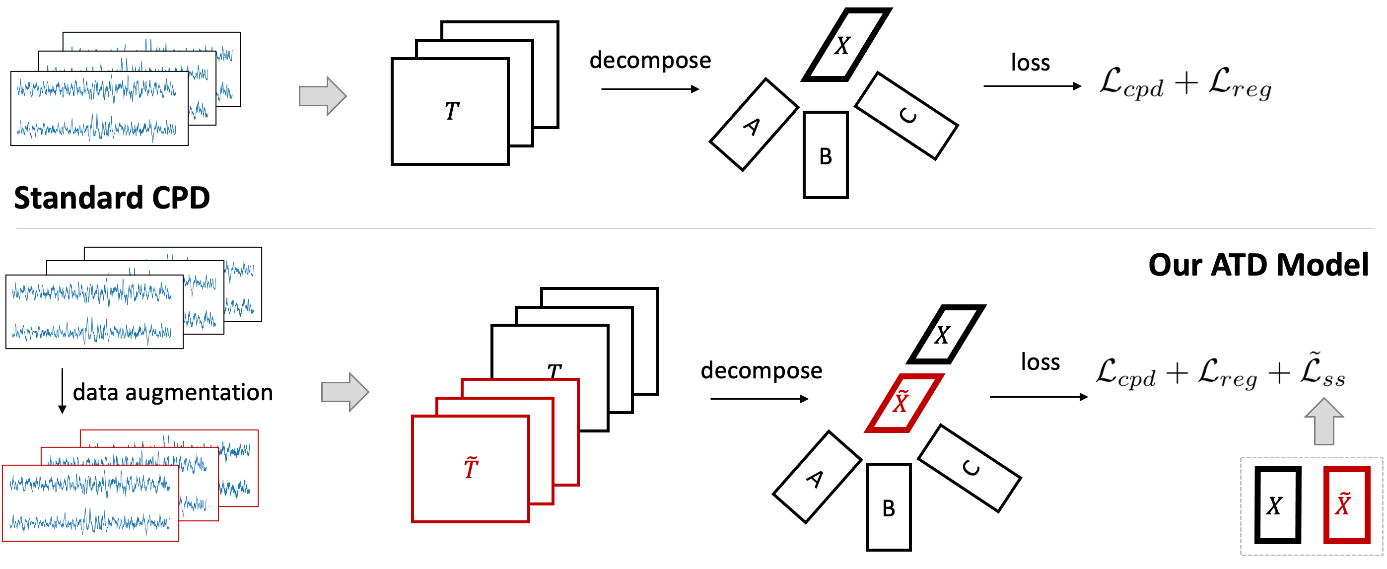
Figure 1: Standard CPD vs Our ATD Model

We show our model in Figure 1. The design is inspired by the recent popularity of SSL. To exploit the latent class information, we introduce class-preserving data augmentation into CPD model and design self-supervised loss to constrain the learned low-rank features (i.e., the coefficient vectors).

Data Augmentation. In general, data augmentation methods are chosen to perturb the raw data while preserving class label information. Given a sample $\mathcal{T}^{(n)}$, we assume that after data augmentation, its perturbation $\tilde{\mathcal{T}}^{(n)}$ preserves the label and admits the component-based representation as in Eqn. (1).

3.1 Self-supervised Loss

The design of our self supervised loss corresponds to the alignment principle, which is based on pairwise feature similarity and dissimilarity. We call a pair of data samples from the same latent class as positive pair, a pair of samples from different latent classes as negative pair and a pair of independent samples (two random samples from the dataset) as random pair. Intuitively, an anchor plus a positive sample composes a positive pair, similarly for negative pairs and random pairs. In this work, our self-supervised loss aims to maximize the feature similarity between positive pairs and minimizes that between negative pairs in an unsupervised way (no labels during optimization).

Formally, let $\mathcal{X}_{p},\mathcal{Y}_{p}$ be discrete random variables (of tensor samples) distributed as $\mathcal{D}_{p},~{}p\in\{1,\dots,P\}$. We want to minimize the following objective when no class labels are given,

$$\mathcal{L}_{ss}= ~{}~{}\mathcal{L}_{pos}+\lambda\mathcal{L}_{neg},$$

where $\lambda\geq 1$ is a hyperparameter and

$$\mathcal{L}_{pos} =-\mathbb{E}\left[\mbox{sim}\left(\mathbf{f}\left(\mathcal{X}_{p}\right),\mathbf{f}\left({\mathcal{Y}_{q}}\right)\right)\mid p=q\right],$$ (3)

$$\mathcal{L}_{neg} =\mathbb{E}\left[\mbox{sim}\left(\mathbf{f}\left(\mathcal{X}_{p}\right),\mathbf{f}\left({\mathcal{Y}_{q}}\right)\right)\mid p\neq q\right].$$

Here $\mathcal{L}_{pos}$ maximizes the feature similarity of positive pairs while $\mathcal{L}_{neg}$ minimizes the feature similarity of negative pairs. $\mathbf{f}(\cdot)$ is the feature extractor, defined in Eqn. (2), and the similarity measure is given by cosine distance, parameterized by two random variables,

$$\mbox{sim}\left(\mathbf{f}\left(\mathcal{X}_{p}\right),\mathbf{f}\left({\mathcal{Y}_{q}}\right)\right)=\left\langle\frac{\mathbf{f}(\mathcal{X}_{p})}{\left\|\mathbf{f}\left(\mathcal{X}_{p}\right)\right\|_{2}},\frac{\mathbf{f}(\mathcal{Y}_{q})}{\left\|\mathbf{f}\left(\mathcal{Y}_{q}\right)\right\|_{2}}\right\rangle.$$

To this end, the key is to implement the self-supervised loss, i.e., Eqn. (3), in an unsupervised setting. Specifically, we want to construct the sampler of positive pairs and the sampler of negative pairs with unlabeled data only. The sampler of positive pairs (in short, positive sampler) can be easily approximated by data augmentation techniques, which provides "surrogate" positive pairs (given any sample as the anchor, we apply data augmentation methods to generate a perturbed data as positive sample, and then the anchor plus the perturbed data is a positive pair). However, the negative sampler is infeasible, without labels. As a compromise, previous works He et al., (2020); Chen et al., (2020) consider using random sampler to replace the negative sampler given that the random sampler can be easily achieved by picking two independent samples from the dataset. However, this practice is shown to induce sampling bias and hurts the learned representation Arora et al., (2019); Chuang et al., (2020) since a random pair may be from the same latent class.

Construction of Negative Sampler.

In this paper, we consider using the law of total probability to construct the negative sampler in a statistical way. Formally, assume $r_{p}$ is the label rate of latent class-$p$ (thus, we have $\sum_{p}r_{p}=1$), we apply the law of total probability and the following holds,

$$\mathbb{E}\left[\mbox{sim}\left(\mathbf{f}\left(\mathcal{X}_{p}\right),\mathbf{f}\left({\mathcal{Y}_{q}}\right)\right)\mid p\neq q\right]=\sum_{p=1}^{P}r_{p}\sum_{q\neq p}\frac{r_{q}}{1-r_{p}}\mathbb{E}_{p,q}\left[\mbox{sim}\left(\mathbf{f}\left(\mathcal{X}_{p}\right),\mathbf{f}\left({\mathcal{Y}_{q}}\right)\right)\right]$$ (4)

$$= -\sum_{p=1}^{P}\frac{r_{p}r_{p}}{1-r_{p}}\mathbb{E}_{p,q}\left[\mbox{sim}\left(\mathbf{f}\left(\mathcal{X}_{p}\right),\mathbf{f}\left({\mathcal{Y}_{q}}\right)\right)\mid p=q\right]+\sum_{p=1}^{P}\sum_{q=1}^{P}\frac{r_{p}r_{q}}{1-r_{p}}\mathbb{E}_{p,q}\left[\mbox{sim}\left(\mathbf{f}\left(\mathcal{X}_{p}\right),\mathbf{f}\left({\mathcal{Y}_{q}}\right)\right)\right]$$

$$= -\mathbb{E}\left[\frac{r_{p}}{1-r_{p}}\mbox{sim}\left(\mathbf{f}\left(\mathcal{X}_{p}\right),\mathbf{f}\left({\mathcal{Y}_{q}}\right)\right)\mid p=q\right]+\mathbb{E}\left[\frac{1}{1-r_{p}}\mbox{sim}\left(\mathbf{f}\left(\mathcal{X}_{q}\right),\mathbf{f}\left({\mathcal{Y}_{q}}\right)\right)\right].$$

Here, the usage of $\mathbb{E}[\cdot]$ means that the expectation is taken over four interdependent random variables, i.e., $p,q,\mathcal{X}_{p},\mathcal{Y}_{q}$, while $\mathbb{E}_{p,q}[\cdot]$ means that $p,q$ is fixed and thus it is only taken over two random variables, i.e., $\mathcal{X}_{p},\mathcal{Y}_{q}$. The result shows that the negative sampler can be equivalently replaced by a weighted combination of the random sampler and positive sampler. Here we do not have access to $r_{p},~{}\forall p$ with unlabeled data, this issue is dealt with later.

Self-supervised Loss.

Consequently, we can reformulate our self-supervised loss as,

$$\mathcal{L}_{ss}= ~{}~{}\mathcal{L}_{pos}+\lambda\mathcal{L}_{neg}$$

$$= -\mathbb{E}\left[\mbox{sim}\left(\mathbf{f}\left(\mathcal{X}_{p}\right),\mathbf{f}\left({\mathcal{Y}_{q}}\right)\right)\mid p=q\right]+\lambda\mathbb{E}\left[\mbox{sim}\left(\mathbf{f}\left(\mathcal{X}_{p}\right),\mathbf{f}\left({\mathcal{Y}_{q}}\right)\right)\mid p\neq q\right]$$ (5)

$$= ~{}\mathbb{E}\left[\frac{\lambda}{1-r_{p}}\mbox{sim}\left(\mathbf{f}\left(\mathcal{X}_{p}\right),\mathbf{f}\left({\mathcal{Y}_{q}}\right)\right)\right]-\mathbb{E}\left[\left(\frac{\lambda r_{p}}{1-r_{p}}+1\right)\mbox{sim}\left(\mathbf{f}\left(\mathcal{X}_{p}\right),\mathbf{f}\left({\mathcal{Y}_{q}}\right)\right)\mid p=q\right].$$ (6)

From Eqn. (5) to Eqn. (6), we use the results in Eqn. (4)

Two-sided Bound.

The above form still requires label rate information, i.e., $r_{p},~{}\forall p$, we therefore consider using the following approximation to the above loss $\mathcal{L}_{ss}$,

$$\mathcal{L}^{\Theta}_{ss}(\gamma)= ~{}(\gamma+1)\mathbb{E}\left[\mbox{sim}\left(\mathbf{f}\left(\mathcal{X}_{p}\right),\mathbf{f}\left({\mathcal{Y}_{q}}\right)\right)\right]-\mathbb{E}\left[\mbox{sim}\left(\mathbf{f}\left(\mathcal{X}_{p}\right),\mathbf{f}\left({\mathcal{Y}_{q}}\right)\right)\mid p=q\right].$$ (7)

Here, $\gamma\geq 0$ is a hyperparameter, while $\mathcal{L}_{ss}$ can be bounded as (derivations in appendix E),

$$C_{1}\mathcal{L}^{\Theta}_{ss}\left(\frac{\lambda-1}{C_{1}}\right)\leq\mathcal{L}_{ss}\leq C_{2}\mathcal{L}^{\Theta}_{ss}\left(\frac{\lambda-1}{C_{2}}\right),~{}C_{1}=1+\max_{p}\frac{\lambda r_{p}}{1-r_{p}},C_{2}=1+\min_{p}\frac{\lambda r_{p}}{1-r_{p}}.$$ (8)

The equivalence is established when $C_{1}=C_{2}$, i.e., the class labels are balanced. To simplify the derivation, we ignore $\lambda$ in the following and let $\gamma$ be a new hyperparameter. Also, the constants $C_{1}$ and $C_{2}$ can be absorbed into a weight hyperparameter $\beta$, given in the next section. This bound implies that, an easy-to-compute $\beta\mathcal{L}_{ss}^{\Theta}(\gamma)$ is often a good approximation of $\mathcal{L}_{ss}$ for some $\beta$. The next section specifies how to compute $\beta\mathcal{L}_{ss}^{\Theta}(\gamma)$ unsupervisedly as our empirical self-supervised loss.

3.2 The Objective of ATD

Empirical Estimator.

We obtain an empirical estimator of $\mathcal{L}^{\Theta}_{ss}$ with Monte Carlo method. Suppose $\mathcal{T}$ and $\tilde{\mathcal{T}}$ are the input tensor and the augmented tensor respectively, and $\mathbf{X}=\mathbf{f}(\mathcal{T}),\tilde{\mathbf{X}}=\mathbf{f}(\tilde{\mathcal{T}})\in\mathbb{R}^{N\times R}$ are the coefficient/feature matrices. We use the row vectors of $\mathbf{X},\tilde{\mathbf{X}}$ to estimate Eqn. (7).

The first term $\mathbb{E}\left[\mbox{sim}\left(\mathbf{f}\left(\mathcal{X}_{p}\right),\mathbf{f}\left({\mathcal{Y}_{q}}\right)\right)\right]$ essentially requires a random sampler, which is approximated by the average cosine similarity of all possible pairs of non-corresponding row vectors of $\mathbf{X},\tilde{\mathbf{X}}$, while the second term $\mathbb{E}\left[\mbox{sim}\left(\mathbf{f}\left(\mathcal{X}_{p}\right),\mathbf{f}\left({\mathcal{Y}_{q}}\right)\right)\mid p=q\right]$ requires a positive sampler, which is estimated by the average cosine similarity of all pairs of corresponding row vectors,

$$\tilde{\mathcal{L}}^{\Theta}_{ss}(\gamma)= ~{}(\gamma+1)\cdot\frac{1}{N(N-1)}\sum_{n=1}^{N}\sum_{s\neq n}^{N}\left\langle\frac{\mathbf{x}^{(n)}}{\|\mathbf{x}^{(n)}\|_{2}},\frac{\tilde{\mathbf{x}}^{(s)}}{\|\tilde{\mathbf{x}}^{(s)}\|_{2}}\right\rangle-\frac{1}{N}\sum_{n=1}^{N}\left\langle\frac{\mathbf{x}^{(n)}}{\|\mathbf{x}^{(n)}\|_{2}},\frac{\tilde{\mathbf{x}}^{(n)}}{\|\tilde{\mathbf{x}}^{(n)}\|_{2}}\right\rangle$$ (9)

$$= ~{}\mbox{Tr}\left(\mathbf{X}^{\top}\mathbf{D}(\mathbf{X})\mathbf{G}(\gamma)\mathbf{D}(\tilde{\mathbf{X}})\tilde{\mathbf{X}}\right),$$

where $\mathbf{D}\left(\mathbf{X}\right)=\mathrm{diag}\left(\frac{1}{\|\mathbf{x}^{(1)}\|_{2}},\cdots,\frac{1}{\|\mathbf{x}^{(N)}\|_{2}}\right)$ is the row-wise scaling matrix and

$$\mathbf{G}(\gamma)=\begin{bmatrix}-\frac{1}{N}&\frac{\gamma+1}{N(N-1)}&\cdots&\frac{\gamma+1}{N(N-1)}\\ \frac{\gamma+1}{N(N-1)}&-\frac{1}{N}&\cdots&\frac{\gamma+1}{N(N-1)}\\ \cdots&\cdots&\cdots&\cdots\\ \frac{\gamma+1}{N(N-1)}&\frac{\gamma+1}{N(N-1)}&\cdots&-\frac{1}{N}\end{bmatrix}.$$

Note that, the form in Eqn. (9) is significantly different from tensor discriminant analysis (Jia et al.,, 2014; Tao et al.,, 2007), which integrates the actual label information as a regularizer and is also different from graph regularized tensor decomposition (Cai et al.,, 2010), which incorporates side information, such as geometrical positions (Maki et al.,, 2018). Compared to standard noise contrastive estimation (NCE) (Gutmann and Hyvärinen,, 2010; Chen et al.,, 2020) in the area of contrastive SSL, our SSL form in Eqn. (9) considers a subtraction form instead of the softmax formulation, making it amenable to quadratic optimization, as we will show in Sec. 3.3.

Overall Objective.

According to Eqn. (8), the self supervised loss ${\mathcal{L}}_{ss}$ is bounded by ${\mathcal{L}}^{\Theta}_{ss}(\gamma)$, while the constants (i.e., $C_{1},C_{2}$) can be absorbed into a weight hyperparameter $\beta$. We let the empirical self-supervised loss, $\tilde{\mathcal{L}}_{ss}{=}\beta\tilde{\mathcal{L}}^{\Theta}_{ss}(\gamma)$. Our objective follows both the fitness (i.e., CPD reconstruction loss) and alignment (i.e., self-supervised loss) principles, while also considering Tikhonov regularization (Golub and Von Matt,, 1997) to constrain the scale of all parameters,

$$\mathcal{L}=\mathcal{L}_{cpd}+\mathcal{L}_{reg}+\tilde{\mathcal{L}}_{ss},$$ (10)

where

$$\mathcal{L}_{cpd} =\left\|\mathcal{T}-\llbracket\mathbf{X},\mathbf{A},\mathbf{B},\mathbf{C}\rrbracket\right\|_{F}^{2}+\left\|\tilde{\mathcal{T}}-\llbracket\tilde{\mathbf{X}},\mathbf{A},\mathbf{B},\mathbf{C}\rrbracket\right\|_{F}^{2},$$

$$\mathcal{L}_{reg} =\alpha\left(\|\mathbf{X}\|_{F}^{2}+\|\tilde{\mathbf{X}}\|_{F}^{2}+\|\mathbf{A}\|_{F}^{2}+\|\mathbf{B}\|_{F}^{2}+\|\mathbf{C}\|_{F}^{2}\right),$$

$$\tilde{\mathcal{L}}_{ss} =\beta\tilde{\mathcal{L}}^{\Theta}_{ss}(\gamma)=\beta\mbox{Tr}\left(\mathbf{X}^{\top}\mathbf{D}(\mathbf{X})\mathbf{G}(\gamma)\mathbf{D}(\tilde{\mathbf{X}})\tilde{\mathbf{X}}\right).$$ (11)

The objective has (i) three hyperparameters, $\gamma,\alpha,\beta>0$; (ii) five factor matrices, $\mathbf{A},\mathbf{B},\mathbf{C}$, $\mathbf{X}$, $\tilde{\mathbf{X}}$.

3.3 Alternating Least Squares Optimization

Ideally, we would like to use alternative least squares (ALS) algorithm (Sidiropoulos et al.,, 2017) for optimizing the objective, where each factor matrix is updated in a sequence by solving least squares subproblems. With large scale tensors, we can also resort to mini-batch stochastic ALS (Cao et al.,, 2020) to reduce memory footprint of the decomposition. However, the objective in Eqn. (11) is non-convex to $\mathbf{X}$ and $\tilde{\mathbf{X}}$, respectively. For addressing the non-convex subproblem, we design an iterative method in this section, which only involves solving least square problems.

Addressing Non-convex Subproblem.

We use the subproblem of $\mathbf{X}$ as an example. Given $\mathbf{A}$, $\mathbf{B}$, $\mathbf{C}$, $\tilde{\mathbf{X}}$ fixed, we want to minimize Eqn. (10) by finding the optimal solution, denotd as $\mathbf{X}^{*}$,

$$\mathbf{X}^{*}\leftarrow \operatorname*{arg\,min}_{{\mathbf{X}}}\left(\left\|{\mathcal{T}}-\llbracket{\mathbf{X}},\mathbf{A},\mathbf{B},\mathbf{C}\rrbracket\right\|_{F}^{2}+\alpha\|{\mathbf{X}}\|_{F}^{2}+\beta\mbox{Tr}\left(\mathbf{X}^{\top}\mathbf{D}(\mathbf{X})\mathbf{G}(\gamma)\mathbf{D}(\tilde{\mathbf{X}})\tilde{\mathbf{X}}\right)\right).$$ (12)

• First, we are interested to find that the matrix-formed problem in Eqn. (12) can be decomposed into row-wise subproblems and to obtain the solution of Eqn. (12), it is suffice to solve each subproblem independently. Let us consider the subproblem of the $k$-th row, which is

  $$\operatorname*{arg\,min}_{\mathbf{x}}\left(\left\|{\mathcal{T}}^{(k)}-\llbracket{\mathbf{x}},\mathbf{A},\mathbf{B},\mathbf{C}\rrbracket\right\|_{F}^{2}+\alpha\|{\mathbf{x}}\|_{F}^{2}+\beta\mbox{Tr}\left(\frac{\mathbf{x}^{\top}}{\|\mathbf{x}\|_{2}}\mathbf{g}^{(k)}\mathbf{D}(\tilde{\mathbf{X}})\tilde{\mathbf{X}}\right)\right),$$ (13)

  where ${\mathcal{T}}^{(k)}$ is the $k$-th slice of ${\mathcal{T}}$, and $\mathbf{g}^{(k)}$ is the $k$-th row of $\mathbf{G}(\gamma)$.

• Here, Eqn. (13) is still non-convex. We let the derivative of Eqn. (13) objective to be zero and arrange the terms, which yields,

  $${\mathbf{x}} =\mathbf{v}_{1}\mathbf{V}_{3}-\frac{\beta\mathbf{v}_{2}}{2\|\mathbf{x}\|_{2}}\left(\mathbf{I}-\frac{\mathbf{x}^{\top}\mathbf{x}}{\|\mathbf{x}\|^{2}_{2}}\right)\mathbf{V}_{3},$$ (14)

  where

  $$\mathbf{v}_{1}=\mathbf{T}^{(k)}_{1}(\mathbf{A}\odot\mathbf{B}\odot\mathbf{C}),~{}~{}~{}~{}\mathbf{v}_{2}=\mathbf{g}^{(k)}\mathbf{D}(\tilde{\mathbf{X}})\tilde{\mathbf{X}},~{}~{}~{}~{}\mathbf{V}_{3}=\left(\mathbf{A}^{\top}\mathbf{A}*\mathbf{B}^{\top}\mathbf{B}*\mathbf{C}^{\top}\mathbf{C}+\alpha\mathbf{I}\right)^{-1}.$$

  Here $\mathbf{x},\mathbf{v}_{1},\mathbf{v}_{2}$ are row vectors and $\mathbf{V}_{3}$ is a matrix. $\mathbf{T}^{(k)}_{1}$ is the $1$-mode unfolding of $\mathcal{T}^{(k)}$, $\odot$ is the Khatri-Rao product and $*$ is the Hadamard product (i.e., element-wise product).

• We consider the following iterative rule and the fixed point is a solution for Eqn. (14), which is a stationary point of Eqn. (13),

  $${\mathbf{x}}_{\mathrm{impr}} =\mathbf{v}_{1}\mathbf{V}_{3}-\frac{\beta\mathbf{v}_{2}}{2\|\mathbf{x}_{\mathrm{init}}\|_{2}}\left(\mathbf{I}-\frac{\mathbf{x}^{\top}_{\mathrm{init}}\mathbf{x}_{\mathrm{init}}}{\|\mathbf{x}_{\mathrm{init}}\|^{2}_{2}}\right)\mathbf{V}_{3}.$$ (15)

  We use an initial guess ${\mathbf{x}}_{\mathrm{init}}$ (obtained by solving Eqn. (13) with while $\beta=0$, which is a least square problem) to start and then we repeat Eqn. (15) for each row (i.e., each $k$) and let the improved guess be the initial guess, ${\mathbf{x}}_{\mathrm{init}}\leftarrow{\mathbf{x}}_{\mathrm{impr}}$, to iteratively improve the result.

Theorem 1 (proof in appendix A) ensures that Eqn. (15) converges linearly if $\beta$ is chosen to be sufficiently small. In appendix B, we verify the liner convergence and also empirically show that one round of Eqn. (15) is sufficient in our experiment, where $\beta=2$. The non-convex subproblem of $\tilde{\mathbf{X}}$ can be solved in the same way.

Theorem 1.

Given non-zero row vectors $\mathbf{v}_{1},\mathbf{v}_{2},\mathbf{u}^{0}\in\mathbb{R}^{d}$, non-singular matrix $\mathbf{V}_{3}\in\mathbb{R}^{d\times d}$ and $\beta>0$. The sequence $\{\mathbf{u}^{t}\}$, generated by $\mathbf{u}^{t+1}=\mathbf{v}_{1}\mathbf{V}_{3}-\frac{\beta\mathbf{v}_{2}}{2\|\mathbf{u}^{t}\|_{2}}\left(\mathbf{I}-\frac{\mathbf{u}^{t\top}\mathbf{u}^{t}}{\|\mathbf{u}^{t}\|_{2}^{2}}\right)\mathbf{V}_{3}$, satisfies,

$$\small\left\|\mathbf{u}^{t+1}-\mathbf{u}^{*}\right\|_{2}\leq\frac{\beta(2m+M)\|\mathbf{v}_{2}\|_{2}\|\mathbf{V}_{3}\|_{F}}{m^{3}}{\left\|\mathbf{u}^{t}-\mathbf{u}^{*}\right\|_{2}},$$

where $\mathbf{u}^{*}$ is the fixed point and $m=\min_{t}\|\mathbf{u}^{t}\|_{2}$, $M=\max_{t}\|\mathbf{u}^{t}\|_{2}$ are the bound of the sequence. With a good $\mathbf{u}^{0}$ and a sufficiently small $\beta$, we can safely assume $0<m\leq M<\infty$.

Optimization Procedures.

To minimize Eqn. (11), we alternatively update $\mathbf{A},\mathbf{B},\mathbf{C}$, $\mathbf{X}$, and $\tilde{\mathbf{X}}$, where each subproblem involves only solving least squares problems with closed-form solutions. With large-scale tensors (as in the experiments), we optimizes the factors in mini-batches. Between mini-batches, the basis factors $\mathbf{A,B,C}$ are shared and updated incrementally. We summarize the algortihms in appendix C. The computation head of the algorithm is matricized tensor times Khatri-Rao product (MTTKRP). The complexity of our optimization algorithm is asymptotically the same as applying CP-ALS, which costs $O(NIJKR)$ to sweep over the whole tensor once.

4 Experiments

This section presents the experimental evaluations. Due to space limitation, additional details, including data augmentations and baseline implementation, are presented in appendix D.

4.1 Experimental Setup

Data Preparation.

We use four real-world datasets: (i) Sleep-EDF (Kemp et al.,, 2000), which contains EOG, EMG and EEG Polysomnography recordings; (ii) human activity recognition (HAR) (Anguita et al.,, 2013) with smartphone accelerometer and gyroscope data; (iii) Physikalisch Technische Bundesanstalt large scale cardiology database (PTB-XL) (Alday et al.,, 2020) with 12-lead ECG signals; (iv) Massachusetts General Hospital (MGH) (Biswal et al.,, 2018) datasets with multi-channel EEG waves. All datasets are split into three disjoint sets (i.e., unlabeled, training and test) by subjects, while training and test sets have labels. Basic statistics are shown in Table 1. All models (baselines and our ATD) use the same augmentation techniques: (a) jittering, (b) bandpass filtering, and (c) 3D position rotation. We provide an ablation study on the augmentation methods in appendix D.5.

Table 1: Dataset Statistics

Name	Data Sample Format	Augmentations	# Unlabeled ($N$)	# Training	# Test	Task	# Class
Sleep-EDF	$I\times J\times K$: 14 $\times$ 129 $\times$ 86	(a), (b)	331,208	42,803	41,078	Sleep Staging	5
HAR	$I\times J\times K$: 18 $\times$ 33 $\times$ 33	(a), (b), (c)	7,352	1,473	1,474	Activity Recognition	6
PTB-XL	$I\times J\times K$: 24 $\times$ 129 $\times$ 75	(a), (b)	17,469	2,183	2,185	Gender Identification	2
MGH	$I\times J\times K$: 12 $\times$ 257 $\times$ 43	(a), (b)	4,377,170	238,312	248,041	Sleep Staging	5

Baseline Methods.

We include the following comparison models from different perspectives:

• Tensor based models: ${\bf\texttt{ATD}}_{ss-}$ is our variant, which removes the self-supervised loss from the objective in Eqn. (10); Stochastic alternating least squares (SALS) applies on the the CPD objective with Tikhonov regularizer, which works on large tensors; Graph regularized SALS (GR-SALS) augments the objective of SALS with a graph regularizer (Maki et al.,, 2018; Cai et al.,, 2010), define as $\mbox{Tr}\left(\mathbf{X}^{\top}\mathbf{G}\mathbf{X}\right)$.

• Self-supervised models: SimCLR-$r$ (Chen et al.,, 2020) and BYOL-$r$ (Grill et al.,, 2020) are two popular SSL models with their own objective functions, where $r$ indicates the size of the output representation.

• Auto-encoder models: AE-$r$ denotes a CNN based autoencoder with mean square error (MSE) reconstruction loss, and $\mbox{AE}_{ss}$-$r$ denotes the same autoencoder model with standard NCE loss in the bottleneck layer, where $r$ is the representation size.

All models use the unlabeled set to train a feature encoder and use training and test sets to evaluate. Note that, deep neural network models use the same CNN backbone. In appendix D.8, we have also compared with two recent supervised tensor learning models, which shows the usefulness of our ATD and the large unlabeled set, especially in low-label rate scenarios.

Evaluation and Environments.

We evaluate model performance mainly based on classification accuracy, where we train an additional logistic classifier (He et al.,, 2020) on top of the feature encoder. Also, for different models, we compare their number of learnable parameters. The experiments are implemented by Python 3.8.5, Torch 1.8.0+cu111 on a Linux workstation with 256 GB memory, 32 core CPUs (3.70 GHz, 128 MB cache), two RTX 3090 GPUs (24 GB memory each). All training is performed on the GPU. For tensor based models, we use $R=32$ and implement the pipeline in CUDA manually, instead of using torch-autograd.

4.2 Experimental Results

This section shows the experimental results on downstream classification. We use all the unlabeled data to train the encoder or feature extractor, and use training data (since Sleep-EDF and MGH datasets have enough training samples, we randomly selected a subset of them) for learning a downstream classifier and use all test data. Each experiment is conducted with five different random seeds and the mean and standard deviations are reported. The metrics are the accuracy and the number of learnable parameters. All models have 32-dim features in the end, except that for two self-supervised baselines and autoencoder models, which have 128-dim options.

Table 2: Result of Downstream Classification (%). The table shows that our ATD can provide comparable or better performance over all baselines with fewer parameters, especially deep learning models. It also shows the usefulness of considering both fitness and alignment as part of the objective.

	Sleep-EDF (5,000)		HAR (1,473)		PTB-XL (2,183)		MGH (5,000)
	Accuracy	# of Params.	Accuracy	# of Params.	Accuracy	# of Params.	Accuracy	# of Params.
Self-sup models:
SimCLR-32	84.98 $\pm$ 0.358	210,384	74.75 $\pm$ 0.723	53,286	69.25 $\pm$ 0.355	200,960	67.34 $\pm$ 0.970	212,624
SimCLR-128	85.19 $\pm$ 0.358	222,768	76.69 $\pm$ 0.697	65,670	68.19 $\pm$ 0.793	237,920	66.98 $\pm$ 1.331	246,608
BYOL-32	84.29 $\pm$ 0.405	211,440	73.71 $\pm$ 2.832	54,342	65.08 $\pm$ 1.535	202,016	68.83 $\pm$ 1.168	214,736
BYOL-128	83.26 $\pm$ 0.337	239,280	71.79 $\pm$ 1.866	82,182	65.49 $\pm$ 0.612	254,432	68.55 $\pm$ 1.339	279,632
Auto-encoders:
AE-32	74.78 $\pm$ 0.723	217,216	63.13 $\pm$ 0.775	62,940	59.01 $\pm$ 0.896	224,528	68.58 $\pm$ 0.427	220,088
AE-128	75.17 $\pm$ 0.897	241,888	60.52 $\pm$ 1.604	87,612	58.29 $\pm$ 0.412	298,352	67.05 $\pm$ 1.375	257,048
$\mbox{AE}_{ss}$-32	80.92 $\pm$ 0.345	217,216	71.70 $\pm$ 2.135	62,940	68.47 $\pm$ 0.231	224,528	71.46 $\pm$ 0.386	220,088
$\mbox{AE}_{ss}$-128	81.84 $\pm$ 0.259	241,888	72.43 $\pm$ 1.370	87,612	68.88 $\pm$ 0.604	298,352	70.19 $\pm$ 0.617	257,048
Tensor models:
SALS	84.27 $\pm$ 0.481	7,328	91.86 $\pm$ 0.295	2,688	69.15 $\pm$ 0.483	7,296	71.93 $\pm$ 0.379	9,984
GR-SALS	84.33 $\pm$ 0.356	7,328	92.33 $\pm$ 0.282	2,688	69.02 $\pm$ 0.477	7,296	72.35 $\pm$ 0.228	9,984
$\texttt{ATD}_{ss-}$	84.19 $\pm$ 0.221	7,328	92.41 $\pm$ 0.391	2,688	69.38 $\pm$ 0.612	7,296	72.78 $\pm$ 0.522	9,984
ATD	85.01 $\pm$ 0.224	7,328	93.35 $\pm$ 0.357	2,688	70.26 $\pm$ 0.523	7,296	74.15 $\pm$ 0.431	9,984
*Parenthesis shows the number of training samples. Our improvements are statistically significant with $p<0.05$ (details in appendix D.7).

4.2.1 Better Classification Accuracy with Fewer Parameters

From Table 2, ATD shows comparable or better performance over the baselines. We have also reported the running time per epoch/sweep in appendix D.7 for all models. Compared to the variant $\texttt{ATD}_{ss-}$, our ATD can improve the accuracy by $1.0\%\sim 1.9\%$, which shows the benefit of the inclusion of self-supervised loss. SALS and $\texttt{ATD}_{ss-}$ have similar performance, while their objectives differ in that $\texttt{ATD}_{ss-}$ considers the Frobenius norm of the augmented data. Thus, their accuracy gap is caused by the use of data augmentation. Also, the experiments show that the fitness and alignment principles are both important. We observe that with a self-supervised loss (i.e., alignment), $\mbox{AE}_{ss}$ can give significant improvement over AE, while ATD shows $\sim 8\%$ accuracy gain over the self-supervised models on MGH dataset, since we can better preserve the data with a reconstruction loss (i.e., fitness).

Moreover, the table shows that tensor based models require fewer parameters, i.e., less than $5\%$ of parameters compared to deep learning models. On HAR, the deep unsupervised models show poor performance due to (i) they may not optimize a large number of parameters on middle-scale dataset; (ii) movement signals in HAR might have few degrees of freedom, which matches well with the low-rank assumption of tensor methods. On large-scale Sleep-EDF, self-supervised models outperforms ATD marginally since they have more parameters thus can capture more information.

4.2.2 Better Performance in Low-label Rate Scenarios

On the MGH dataset, we also show the effect of varying the amount of training data in Figure 2. We include an end-to-end convolutional neural network (CNN) model based on (Biswal et al.,, 2018), called Reference CNN, which is a supervised model and only uses the training and test sets. To be more readable, we separate the comparison figure into two sub-figures: the left compares our ATD model with self-supervised and auto-encoder baselines and the right one compares ATD with tensor baselines and the reference model, and the scale of y-axis on two sub-figures are the same.

We find that all unsupervised models outperform the supervised reference CNN model in scenarios with fewer training samples. With more training data, the performance of all models get improved, especially the reference CNN model, which can optimize the encoder and predictive layers in an end-to-end way and finally outperforms our ATD when more training samples is available.

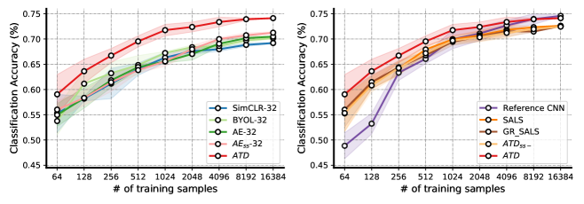
Figure 2: Varying the # of Training Data

4.2.3 Stable Results with Hyperparameter Variation

For a comprehensive evaluation, we also conduct ablation studies on the effect of the data augmentation methods and on hyperparameters. Due to space limitation, we move the experimental settings and results to appendix D.6, while summarizing the general conclusions here: (i) with more diverse data augmentation methods, the final results are relatively better; (ii) with a larger rank $R$, the performance will be better generally; (iii) our ATD is not sensitive hyperparameters $\alpha,\beta,\gamma$.

5 Conclusion

This paper introduces the concept of self-supervised learning for tensors and proposes Augmented Tensor Decomposition (ATD) and the ALS-based optimization. We show that by explicitly contrasting positive and negative samples, the decomposition results are more aligned with downstream classification. On four real-world datasets, we show the advantages of our model over various unsupervised models and with fewer training data, our model even outperforms the reference supervised models.

Compared to deep learning methods, tensor based models are not as flexible in processing multimodal and diverse inputs, such as natural images. However, applying tensor decomposition on the outputs of earlier layers of pre-trained deep neural networks may be a feasible way to address the weaknesses. This direction would be interesting for future work.

Appendix A Proof of theorem

Proof.

We provide the proof below (first by submultiplicativity),

$$\left\|\mathbf{u}^{t+1}-\mathbf{u}^{*}\right\|_{2} =\left\|\frac{\beta\mathbf{v}_{2}}{2\|\mathbf{u}^{*}\|_{2}}\left(\mathbf{I}-\frac{\mathbf{u}^{*\top}\mathbf{u}^{*}}{\|\mathbf{u}^{*}\|_{2}^{2}}\right)\mathbf{V}_{3}-\frac{\beta\mathbf{v}_{2}}{2\|\mathbf{u}^{t}\|_{2}}\left(\mathbf{I}-\frac{\mathbf{u}^{t\top}\mathbf{u}^{t}}{\|\mathbf{u}^{t}\|_{2}^{2}}\right)\mathbf{V}_{3}\right\|_{2}$$

$$\leq\left\|\frac{\beta\mathbf{v}_{2}}{2}\right\|_{2}\|\mathbf{V}_{3}\|_{F}\left\|\frac{1}{\|\mathbf{u}^{*}\|_{2}}\left(\mathbf{I}-\frac{\mathbf{u}^{*\top}\mathbf{u}^{*}}{\|\mathbf{u}^{*}\|_{2}^{2}}\right)-\frac{1}{\|\mathbf{u}^{t}\|_{2}}\left(\mathbf{I}-\frac{\mathbf{u}^{t\top}\mathbf{u}^{t}}{\|\mathbf{u}^{t}\|_{2}^{2}}\right)\right\|_{2}$$

$$=\left\|\frac{\beta\mathbf{v}_{2}}{2}\right\|_{2}\|\mathbf{V}_{3}\|_{F}\left\|\left(\frac{1}{\|\mathbf{u}^{*}\|_{2}}-\frac{1}{\|\mathbf{u}^{t}\|_{2}}\right)+\left(\frac{\mathbf{u}^{t\top}\mathbf{u}^{t}}{\|\mathbf{u}^{t}\|_{2}^{3}}-\frac{\mathbf{u}^{*\top}\mathbf{u}^{*}}{\|\mathbf{u}^{*}\|_{2}^{3}}\right)\right\|_{2}.$$

Then, we decompose the last term into two parts and have

$$\frac{1}{\|\mathbf{u}^{*}\|_{2}}-\frac{1}{\|\mathbf{u}^{t}\|_{2}} =\frac{\|\mathbf{u}^{t}\|_{2}-\|\mathbf{u}^{*}\|_{2}}{\|\mathbf{u}^{*}\|_{2}\|\mathbf{u}^{t}\|_{2}}\leq\frac{\|\mathbf{u}^{t}-\mathbf{u}^{*}\|_{2}}{\|\mathbf{u}^{*}\|_{2}\|\mathbf{u}^{t}\|_{2}}\leq\frac{\|\mathbf{u}^{t}-\mathbf{u}^{*}\|_{2}}{m^{2}},$$

$$\frac{\mathbf{u}^{t\top}\mathbf{u}^{t}}{\|\mathbf{u}^{t}\|_{2}^{3}}-\frac{\mathbf{u}^{*\top}\mathbf{u}^{*}}{\|\mathbf{u}^{*}\|_{2}^{3}} =\left(\frac{\mathbf{u}^{t\top}\mathbf{u}^{t}}{\|\mathbf{u}^{t}\|_{2}^{3}}-\frac{\mathbf{u}^{*\top}\mathbf{u}^{t}}{\|\mathbf{u}^{t}\|_{2}^{3}}\right)+\left(\frac{\mathbf{u}^{*\top}\mathbf{u}^{t}}{\|\mathbf{u}^{t}\|_{2}^{3}}-\frac{\mathbf{u}^{*\top}\mathbf{u}^{*}}{\|\mathbf{u}^{t}\|_{2}^{3}}\right)+\left(\frac{\mathbf{u}^{*\top}\mathbf{u}^{*}}{\|\mathbf{u}^{t}\|_{2}^{3}}-\frac{\mathbf{u}^{*\top}\mathbf{u}^{*}}{\|\mathbf{u}^{*}\|_{2}^{3}}\right)$$

$$=\frac{(\mathbf{u}^{t\top}-\mathbf{u}^{*\top})\mathbf{u}^{t}}{\|\mathbf{u}^{t}\|_{2}^{3}}+\frac{\mathbf{u}^{*\top}(\mathbf{u}^{t}-\mathbf{u}^{*})}{\|\mathbf{u}^{t}\|_{2}^{3}}+\frac{\|\mathbf{u}^{*}\|^{2}_{2}(\|\mathbf{u}^{*}\|_{2}^{3}-\|\mathbf{u}^{t}\|^{3}_{2})}{\|\mathbf{u}^{t}\|_{2}^{3}\|\mathbf{u}^{*}\|_{2}^{3}}$$

$$\leq\frac{\|\mathbf{u}^{t}-\mathbf{u}^{*}\|_{2}}{m^{2}}+\frac{M\|\mathbf{u}^{t}-\mathbf{u}^{*}\|_{2}}{m^{3}}+\frac{(M+2m)\|\mathbf{u}^{t}-\mathbf{u}^{*}\|_{2}}{m^{3}}.$$

The proof is complete by triangular inequality. ∎

Appendix B Analysis of the Iterative Rule

In this section, we study how many rounds of the iterative rules are needed to achieve a good classification result. This study is conducted on HAR and Sleep-EDF with five random seeds.

Linear Convergence Speed. First, we study the convergence speed (when $\beta=2$). We consider two scenarios: (Scenario 1) when the bases $\{\mathbf{A},\mathbf{B},\mathbf{C}\}$ are initialized as random matrices; (Scenario 2) when the based $\{\mathbf{A},\mathbf{B},\mathbf{C}\}$ are already learned. We use the average relative difference (of the F-norm) as the convergence measure, i.e., $\frac{1}{N}\sum_{k=1}^{N}\frac{\|\mathbf{x}^{(k)}_{t+1}-\mathbf{x}^{(k)}_{t}\|}{\|\mathbf{x}^{(k)}_{t}\|}=\frac{1}{N}\sum_{k=1}^{N}\frac{\|\mathbf{x}^{(k)}_{\mathrm{impr}}-\mathbf{x}^{(k)}_{\mathrm{init}}\|}{\|\mathbf{x}^{(k)}_{\mathrm{init}}\|}$, where $\mathbf{x}^{(k)}$ means the $k$-th row of $\mathbf{X}$ and $t$ means the number of rounds of the iterative rule. We test on $t=1,2,3,4,8$. The comparison is shown in Figure 3. Both scenarios verify the linear convergence speed.

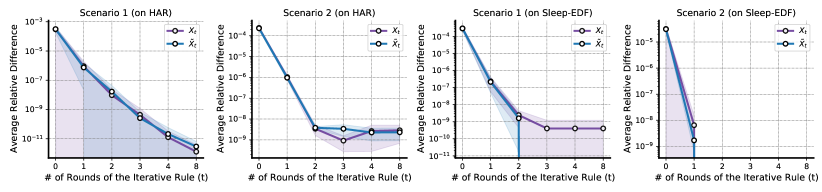
Figure 3: Verification of Convergence Speed. When the # of iteration $t$ becomes larger, the average relative difference can exceed the minimum precision and go to zero (like Scenario 2 on Sleep-EDF).

One Round is Enough. We consider the performance of downstream classification with different rounds of iterative rules. The results are shown in Table 3 and Table 4.

Table 3: Performance with Different Rounds (on HAR)

# of rounds (t)	1	2	3	4	8
time per sweep	8.774s	10.316s	11.224s	12.781s	17.402s
accuracy (%)	93.30 $\pm$ 0.413	93.35 $\pm$ 0.172	93.35 $\pm$ 0.150	93.35 $\pm$ 0.122	93.35 $\pm$ 0.122

Table 4: Performance with Different Rounds (on Sleep-EDF)

# of rounds (t)	1	2	3	4	8
time per sweep	148.375s	160.924s	173.361s	188.193s	242.386s
accuracy (%)	85.25 $\pm$ 0.209	85.33 $\pm$ 0.173	85.31 $\pm$ 0.178	85.31 $\pm$ 0.177	85.31 $\pm$ 0.177

We observe that with an increasing number of rounds of iterative rule, the classification results will not improve further, however, the time consumption increases. Thus, we use only one round of the iterative rule in our experiments.

Appendix C Algorithm

For small tensors, the algorithmic pipeline is presented in Algorithm 1. For large tensors, we use mini-batch alternating least squares optimization in Algorithm 2.

1Input: Data tensor $\mathcal{T}\in\mathbb{R}^{N\times I\times J\times K}$; initialized $\mathbf{A},\mathbf{B},\mathbf{C},\tilde{\mathbf{X}},\mathbf{X}$; other hyperparameters $\alpha,\beta,\gamma$;

2 Obtain the augmented tensor $\tilde{\mathcal{T}}$;

3 repeat

4       Use $\mathbf{A},\mathbf{B},\mathbf{C},\tilde{\mathbf{X}}$ to update $\mathbf{X}$ by our iterative rules (one iteration) in Eqn. (15);

5       Use $\mathbf{A},\mathbf{B},\mathbf{C},\mathbf{X}$ to update $\tilde{\mathbf{X}}$ by our iterative rules (one iteration) in Eqn. (15);

6       Use $\mathbf{B},\mathbf{C},\mathbf{X},\tilde{\mathbf{X}}$ to update $\mathbf{A}$ by solving least square problem;

7       Use $\mathbf{A},\mathbf{C},\mathbf{X},\tilde{\mathbf{X}}$ to update $\mathbf{B}$ by solving least square problem;

8       Use $\mathbf{A},\mathbf{B},\mathbf{X},\tilde{\mathbf{X}}$ to update $\mathbf{C}$ by solving least square problem;

9      

10until max sweep exceeds or change of loss $<0.1\%$ within 3 consecutive sweeps;

Output: the learned bases $\{\mathbf{A},\mathbf{B},\mathbf{C}\}$.

Algorithm 1 Alternating Least Squares

1Input: Data tensor $\mathcal{T}\in\mathbb{R}^{N\times I\times J\times K}$; initialized $\{\mathbf{A}^{1},\mathbf{B}^{1},\mathbf{C}^{1}\}$; batch size $b$; learning rate $\eta$; other hyperparameters $\alpha,\beta,\gamma$; initial counter $l=1$;

2 repeat

3       shuffle the data tensor $\mathcal{T}$;  $/*$ start a new sweep $*/$

4       for a tensor batch $\mathcal{T}^{l}\in\mathbb{R}^{b\times I\times J\times K}$ and its augmentation $\tilde{\mathcal{T}}^{l}$ do

5             use $\mathbf{A}^{l},\mathbf{B}^{l},\mathbf{C}^{l}$ to initialize $\mathbf{X}$ based on $\mathcal{T}^{l}$;

6             use $\mathbf{A}^{l},\mathbf{B}^{l},\mathbf{C}^{l}$ to initialize $\tilde{\mathbf{X}}$ based on $\tilde{\mathcal{T}}^{l}$;

7             Use $\mathbf{A}^{l},\mathbf{B}^{l},\mathbf{C}^{l},\tilde{\mathbf{X}}$ to update $\mathbf{X}$ by our iterative rules (one iteration) in Eqn. (15);

8             Use $\mathbf{A}^{l},\mathbf{B}^{l},\mathbf{C}^{l},\mathbf{X}$ to update $\tilde{\mathbf{X}}$ by our iterative rules (one iteration) in Eqn. (15);

9             Use $\mathbf{B}^{l},\mathbf{C}^{l},\mathbf{X},\tilde{\mathbf{X}}$ to obtain $\mathbf{A}^{l+1}$ by solving least square problem;

10             Use $\mathbf{A}^{l+1},\mathbf{C}^{l},\mathbf{X},\tilde{\mathbf{X}}$ to obtain $\mathbf{B}^{l+1}$ by solving least square problem;

11             Use $\mathbf{A}^{l+1},\mathbf{B}^{l+1},\mathbf{X},\tilde{\mathbf{X}}$ to obtain $\mathbf{C}^{l+1}$ by solving least square problem;

12             $l=l+1$  $/*$ increment the counter $*/$;

13       end for

14      

15until max sweep exceeds or change of loss $<0.1\%$ within 3 consecutive sweeps;

Output: the learned bases $\{\mathbf{A}^{L},\mathbf{B}^{L},\mathbf{C}^{L}\}$.

Algorithm 2 Mini-batch Alternating Least Squares

Appendix D Experimental Details

D.1 Dataset Processing

Sleep-EDF is public, which contains 153 full-night EEG (from Fpz-Cz and Pz-Oz electrode locations), EOG (horizontal), and submental chin EMG recordings, under Open Data Commons Attribution License v1.0 and MGH Sleep is provided by (Biswal et al.,, 2018), where F3-M2, F4-M1, C3-M2, C4-M1, O1-M2, O2-M1 channels are used, containing 6,478 recordings. These two EEG datasets are processed in a similar way. First, the raw data are (long) recordings of each subject. On subject-level, these recordings are categorized into unlabeled and labeled sets by $90\%:10\%$. Then the labeled sets are further separated into training and test by $5\%:5\%$. Next, within each set (unlabeled, training, test), recordings are further segmented into disjoint 30-second-long periods, which are the data samples in our study. Each data sample is represented as a matrix, channel by timestamp, and they are associated with one of five sleep stages, Awake (W), Non-REM stage 1 (N1), Non-REM stage 2 (N2), Non-REM stage 3 (N3), and REM stage (R). HAR is also public, collected as 3-axial linear acceleration and 3-axial angular velocity at a constant rate of 50Hz by the embedded accelerometer and gyroscope. It has been randomly partitioned into 70% and 30%. We use 70% as the unlabeled data (labels removed) and split the other part: 15% as training data and 15% as the test data. The license of this dataset is included in their citation. PTB-XL is a public ECG dataset, which contains 21,837 clinical 12-lead ECGs (male: 11,379 and female: 10,458) of 10-second length with a sampling frequency of 500 Hz. We randomly split the dataset into unlabeled (remove the labels) and labeled sets by $90\%:10\%$; then the labeled sets are further separated into training and test by $5\%:5\%$. This dataset is under Open BSD 3.0.

All datasets are de-identified (e.g., no names, no locations), and there is no offensive content. All the labels are also provided along with the datasets. The label distributions are shown below.

Table 5: Class Label Distribution

Name	Label Distribution
Sleep-EDF	W: 68.8%, N1: 5.2%, N2: 16.6%, N3: 3.2%, R: 6.2%
HAR	Walk: 16.72%, Walk upstairs: 14.99%, Walk downstairs: 13.65%,
	Sit: 17.25%, Stand: 18.51%, Lay: 18.88%
PTB-XL	Male: 52.11%, Female: 47.89%
MGH Sleep	W: 44.3%, N1: 9.9%, N2: 14.4%, N3: 17.6%, R: 13.8%

D.2 STFT Transform

We find that directly using the raw data (spatial information) does not provide good results, even for the deep learning models. Thus, we take Short-Time Fourier Transforms (STFT) as a preprocessing step. From a single channel, we can extract both the amplitude and phase information, which is then stacked together as two different channels. After STFT, each data sample becomes a three-order tensor, channel by frequency by timestamp. The FFT size is 256 and hop length is 32 for Sleep-EDF; the FFT size is 64 and hop length is 2 for HAR; the FFT size is 256 and hop length is 64 for PTB-XL; and the FFT size is 512 and hop length is 128 for MGH. We use these third-order tensors as final input data samples for all models.

D.3 Data Augmentation

In our work, we build our feature extractor $\mathbf{f}(\cdot)$ from tensor decomposition tool, which may not be as expressive/flexible as deep neural networks in SSL, and thus we also ask the augmentation methods to allow a similar component-based representation for the perturbed data. Use EEG signals as an example, we consider jittering and bandpass filtering as two augmentation methods in the experiments, which perturb the signal frequency information and will not significantly change the low-rank structure of the data.

As mentioned in the main text, we consider three different augmentation methods: (i) Jittering adds additional perturbations to each sample. We consider both high and low-frequency noise on each channel independently. For high-frequency noise, we first generate a noisy sequence $\mathbf{s}$, which has the same length as the signal channel, and each element of $\mathbf{s}$ is i.i.d. sampled from a uniform distribution $U[-1,1]$. We then control the amplitude of $\mathbf{s}$ by the noisy degree $d\in\mathbb{R}$. Finally, we add the scaled noisy sequence $d\cdot\mathbf{s}$ to the channel. In the experiment, $d=0.05$ for Sleep-EDF, $d=0.002$ for HAR, $d=0.001$ for PTB-XL and $d=0.01$ for MGH. For low-frequency noise, we generate a short noisy sequence (the length is randomly sampled from a uniform distribution $U[100,\mbox{length of channel}]$) in the same way and then use scipy.interpolate.interp1d to interpolate the noisy sequence to be at the same length as the channel. The choice of high-frequency noise or low-frequency noise, or both are coin-tossed with equal probability. (ii) Bandpass filtering reduces signal noise. We use the order-1 Butterworth filter by scipy.signal.butter to preserve only the within-band frequency information. The high-pass and low-pass are $(1Hz,30Hz)$ and $(10Hz,49Hz)$ for Sleep-EDF, $(1Hz,20Hz)$ and $(5Hz,24.5Hz)$ for HAR, $(1Hz,30Hz)$ and $(10Hz,50Hz)$ for PTB-XL, $(1Hz,30Hz)$ and $(10Hz,50Hz)$ for MGH. Low-pass or high-pass or both are selected with equal probability. Also, the bandpass filtering is applied to each channel independently. The intuition is that the low-pass signals and high-pass signals might be both useful. (iii) 3D position rotation is an augmentation technique used only for HAR datasets, which have x-y-z axis information from accelerometer and gyroscope sensors. We apply a 3D x-y-z coordinate system rotation by a rotation matrix to mimic different cellphone positions. All augmentation methods are applied in sequence (i) (ii) (iii). The STFT is performed after the data augmentation.

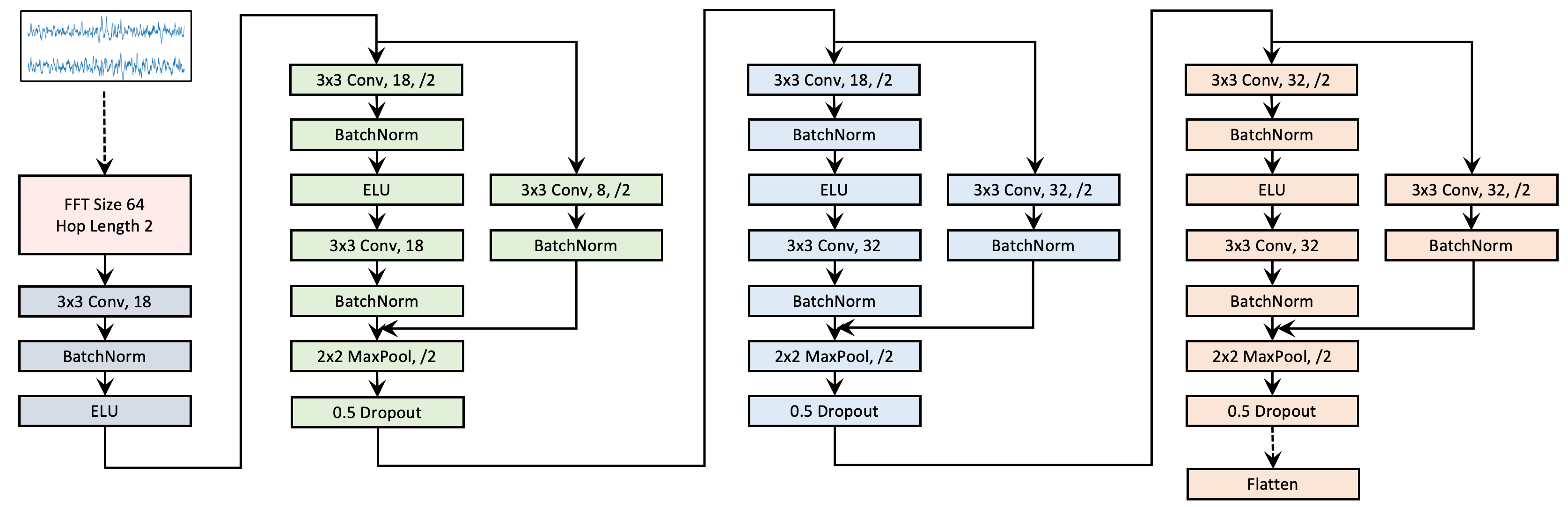
Figure 4: Backbone CNN Architecture (HAR). The architectures for other three datasets are similar.

D.4 Implementation

Since all deep learning baselines are based on CNN, we use the same backbone model, shown in Figure 4. The model is adopted from (Cheng et al.,, 2020). Based on the backbone model, we add a fully connected layer for the reference CNN model, add non-linear layers for self-supervised models (they also have their respective loss), and add corresponding deconvolutional layers for autoencoder models. The reference CNN models is end-to-end, and they are trained on the training set; other baselines learn a low-dimensional feature extractor from an unlabeled set, and then a logistic classifier is trained on the training set, on top of the feature extractor. Without loss of generality, we use $128$ as batch size. For deep learning models, we use Adam optimizer with a learning rate $1\times 10^{-3}$ and weight decaying $5\times 10^{-4}$. We use $2\times 10^{-3}$ as the learning rate for our ATD. Since the paper deals with unsupervised learning and uses standard logistic regression (sklearn.linear_model.LogisticRegression) to evaluate, the hyperparameters of all models (except supervised model) are chosen based on the classification performance on the training data. For our ATD model, by default, we use $R=32,\alpha=1\times 10^{-3},\beta=2$, $\gamma=b$ (which is the batch size), and all the reference configurations for each experiments are listed in code appendix. The choice of $R$ depends on the trade-off between model fitness and time complexity. Specifically, a larger $R$ means better fitness and more preserved information in the extracted representations, while the number of learnable parameters and time complexity also increases linearly with $R$. In our paper, we run simple CP decomposition on a small subset of the tensor and monitor the fitness curve. We find that the fitness does not improve much around $R=32$ for all datasets (which means the real tensor might have a smaller rank and the residual part might be just noise). Thus, we choose $R=32$ throughout the paper.

D.5 Ablation Studies on Data Augmentation

Effect of High-quality Data Augmentations.

We study the effects of high-quality data augmentation methods. Let us assume (a): jittering, (b): bandpass filtering, (c): 3D position rotation. We test on different combinations of the augmentation methods. The experiments are conducted on two datasets: (i) for the MGH dataset, we use 50,000 unlabeled data, 5,000 training samples, and all test samples; (ii) for the HAR dataset, we use all data. We use 128 as the batch size for MGH Sleep, 64 for HAR, and $R=32$ as the tensor rank.

Table 6: Ablation Studies on Data Augmentation (MGH Sleep)

Method	Acc (%)	Method	Acc (%)	Method	Acc (%)
(a)	72.53 $\pm$ 0.652	(b)	73.60 $\pm$ 0.270	(a)+(b)	74.15 $\pm$ 0.203

Table 7: Ablation Studies on Data Augmentation (HAR)

Method	Acc (%)	Method	Acc (%)	Method	Acc (%)
(a)	92.06 $\pm$ 0.621	(a)+(b)	92.70 $\pm$ 0.266	(a)+(b)+(c)	93.35 $\pm$ 0.357
(b)	91.99 $\pm$ 0.274	(a)+(c)	92.93 $\pm$ 0.590	/	/
(c)	92.29 $\pm$ 0.330	(b)+(c)	92.26 $\pm$ 0.479	/	/

Table 6 and Table 7 conclude that the augmentation methods influence the final classification results. However, for different datasets, the effects are different. We observe that for the MGH Sleep dataset, bandpass filtering works better than jittering. In HAR, combinations of augmentations work better than the individual augmentations. Overall, we find that with more diverse data augmentation methods, the final results are relatively better. The study of how to choose/design (or even automatically generate) better augmentation techniques will be our future work.

Impact of Low-quality Data Augmentations.

We also study the impact of low-quality data augmentations. We use the SALS model (mini-batch tensor baseline without data augmentation) and our ATD as the reference models and conduct the following experiments on MGH and HAR:

• MGH-d: we change the $d$ values for the jittering data augmentation, $d$ means the ratio of the amplitude of the high/low frequency noise over the amplitude of the signal.

• MGH-(A): on MGH data, we set the degree of the jittering method to an unrealistic value $d=1$ as the low-quality augmentation method, meaning that the magnitude of the noise is the same as the magnitude of the signals. We keep the bandpass filtering unchanged.

• MGH-(B): on MGH data, we randomly create a bandpass filter from $(1Hz,10Hz)$ or $(30Hz,50Hz)$ as the low-quality augmentation method, which drops the critical middle-band information. We keep the jittering unchanged.

• MGH-(C): on MGH data, we combine the above two low-quality augmentation methods.

• HAR-(A)(B)(C): follow the similar low-quality data augmentation method design on HAR. For (B), we use $(1Hz,5Hz)$ and $(20Hz,24.5Hz)$ as the low-quality bandpass.

The performances are shown in Table 8. We find that low-quality data augmentations will hurt the learned tensor bases and hinder the downstream classification. With $d$ changing from $0.02$ to $5$, the jittering method becomes more unrealistic and the generated samples deviate from the real signal data distribution. Thus, we can find that the final classification performance also becomes worse gradually. If all data augmentation methods are of low-quality, the performance cannot surpass the base SALS model. We also find that the performance drop is not significant. The reason might be that even the augmentation methods are of low-quality, the Frobenius loss can still enforce the model to learn decent subspaces for better fitness and find generic low-rank features (opposed to the classification-oriented low-rank features), in this case, the features only follow fitness principle not the alignment principle, so the performance will be similar compared to SALS.

Table 8: Performance of Low-quality Data Augmentation (on MGH and HAR)

MGH	$d=0.02$	$d=0.05$	$d=0.1$	$d=0.5$	$d=5$
Accuracy	74.18 $\pm$ 0.326	74.10 $\pm$ 0.302	73.85 $\pm$ 0.530	73.39 $\pm$ 0.493	72.18 $\pm$ 0.676
MGH	SALS	ATD	(A)	(B)	(C)
Accuracy	71.93 $\pm$ 0.379	74.15 $\pm$ 0.431	72.73 $\pm$ 0.624	72.10 $\pm$ 0.719	70.75 $\pm$ 0.771
HAR	SALS	ATD	(A)	(B)	(C)
Accuracy	91.86 $\pm$ 0.295	93.35 $\pm$ 0.357	92.04 $\pm$ 0.308	92.48 $\pm$ 0.469	91.43 $\pm$ 0.835

D.6 Ablation Studies on Hyperparameters

This section conducts ablation studies for decomposition rank $R$ and other hyperparameters, $\alpha$, $\beta$, $\gamma$. The experiments are conducted on Sleep-EDF with 50,000 random unlabeled data, 5,000 random training samples, and all test samples, and the HAR dataset.

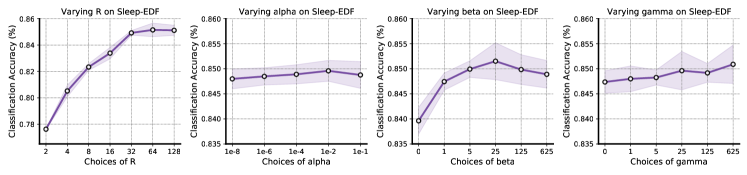
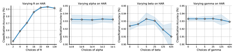
Figure 5: Ablation Studies on Hyperparameters

Table 9: Comparison with Tensor-based Methods with Different R (on HAR)

Model	$R=8$	$R=16$	$R=32$	$R=64$	$R=128$
SALS	69.59 $\pm$ 0.526	83.92 $\pm$ 0.416	91.84 $\pm$ 0.295	91.89 $\pm$ 0.217	91.55 $\pm$ 0.388
GR-SALS	69.62 $\pm$ 0.458	84.20 $\pm$ 0.727	92.33 $\pm$ 0.282	92.28 $\pm$ 0.359	91.84 $\pm$ 0.534
$\texttt{ATD}_{ss-}$	70.27 $\pm$ 0.488	84.84 $\pm$ 0.557	92.41 $\pm$ 0.391	92.71 $\pm$ 0.243	92.32 $\pm$ 0.330
ATD	71.91 $\pm$ 0.253	85.61 $\pm$ 0.294	93.35 $\pm$ 0.357	93.43 $\pm$ 0.411	92.97 $\pm$ 0.273

Table 10: Comparison with Tensor-based Methods with Different R (on Sleep-EDF)

Model	$R=8$	$R=16$	$R=32$	$R=64$	$R=128$
SALS	81.26 $\pm$ 0.345	82.59 $\pm$ 0.638	84.27 $\pm$ 0.481	84.55 $\pm$ 0.527	84.49 $\pm$ 0.317
GR-SALS	81.72 $\pm$ 0.664	82.74 $\pm$ 0.481	84.33 $\pm$ 0.356	84.87 $\pm$ 0.486	84.90 $\pm$ 0.781
$\texttt{ATD}_{ss-}$	81.27 $\pm$ 0.568	82.5 $\pm$ 0.674	84.19 $\pm$ 0.221	84.47 $\pm$ 0.258	84.44 $\pm$ 0.577
ATD	82.49 $\pm$ 0.464	83.31 $\pm$ 0.591	85.01 $\pm$ 0.224	85.30 $\pm$ 0.483	85.32 $\pm$ 0.305

The results are shown in Figure 5. First, we can conclude that with a larger decomposition rank $R$, the performance will be better generally. Though we observe that the performance worsens from $R=64$ to $R=128$, with limited training data, if the representation size (equals to $R$) becomes larger, the logistic regression model can overfit. We compare our model to other tensor-based methods with $R=8,16,32,64,128$ and the Table 9 and Table 10 shows that ATD outperforms the tensor baselines consistently with different R.

Also, we find that the choices of $\alpha$ do not affect the final performance a lot. Finally, we find that it is easy for users to select the $\beta$ values from a large range in general. For example, selecting a $\beta\in[5,125]$ would guarantee good results on Sleep-EDF while on HAR, the selection range is $[5,25]$. The choice of $\beta$ does affect the final performance, but it is not tricky to search for a $\beta$ for good performance. We also find that the accuracy score first increases then decreases with an increasing value of $\beta$. The reason might be that a large $\beta$ will negatively affect the fitness loss.

D.7 Statistical Testing and Running Time Comparison

In this section, we conduct T-test on the result in Section 4.2.1 and calculate the p-values in the parenthesis of Table 11 and Table 12 (the experimental results are copied from Table 2). Commonly, a p-value smaller than 0.05 would be considered as significant. We can see that our model show significant performance gain over all baselines on all tasks.

We have also reported the running time per sweep/epoch in the tables. When recording the running time, we duplicated the environment mentioned in Section 4.1, stopped other programs and ran all the models one by one on GPUs. We record the first 8 sweeps/epochs of all models and drop the first 3 sweeps (since they might be unstable). The average running time of the last 5 epochs are reported in Table 11 and Table 12 while the accuracy results are from Table 2. Note that on HAR, PTB-XL and Sleep-EDF, all methods use 128 as the batch size and on MGH, all methods use 512 as the batch size. The tensor based methods all use $R=32$ as the rank. We can conclude that the tensor based methods are generally more time-efficient than the deep learning methods with fewer parameters. Since our model ATD and the variant $\texttt{ATD}_{ss-}$ use the augmented tensors, they cost more compared to other tensor based methods (since the size of training tensors doubles), however, we also observe empirically that they can converge faster with around half number of the epochs.

Table 11: Result Significance and Running Time (%) for Sleep-EDF and HAR

	Sleep-EDF (5,000)			HAR (1,473)
	Accuracy	# of Params.	Time per sweep	Accuracy	# of Params.	Time per sweep
Self-sup models:
SimCLR-32	84.98 $\pm$ 0.358	210,384	260.299s	74.75 $\pm$ 0.723	53,286	8.459s
SimCLR-128	85.19 $\pm$ 0.358	222,768	265.809s	76.69 $\pm$ 0.697	65,670	8.532s
BYOL-32	84.29 $\pm$ 0.405	211,440	255.614s	73.71 $\pm$ 2.832	54,342	8.430s
BYOL-128	83.26 $\pm$ 0.337	239,280	257.266s	71.79 $\pm$ 1.866	82,182	8.478s
Auto-encoders:
AE-32	74.78 $\pm$ 0.723	217,216	153.684s	63.13 $\pm$ 0.775	62,940	7.530s
AE-128	75.17 $\pm$ 0.897	241,888	156.813s	60.52 $\pm$ 1.604	87,612	7.662s
$\mbox{AE}_{ss}$-32	80.92 $\pm$ 0.345	217,216	301.773s	71.70 $\pm$ 2.135	62,940	7.765s
$\mbox{AE}_{ss}$-128	81.84 $\pm$ 0.259	241,888	307.546s	72.43 $\pm$ 1.370	87,612	7.804s
Tensor models:
SALS	84.27 $\pm$ 0.481 (0.0041)	7,328	86.281s	91.86 $\pm$ 0.295 (2e-5)	2,688	7.535s
GR-SALS	84.33 $\pm$ 0.356 (0.0019)	7,328	109.916s	92.33 $\pm$ 0.282 (0.0003)	2,688	7.829s
$\texttt{ATD}_{ss-}$	84.19 $\pm$ 0.221 (9e-5)	7,328	147.568s	92.41 $\pm$ 0.391 (0.0011)	2,688	8.604s
ATD	85.01 $\pm$ 0.224	7,328	148.375s	93.35 $\pm$ 0.357	2,688	8.672s
result format: mean $\pm$ standard deviation (p-value)

Table 12: Result Significance and Running Time (%) for PTB-XL and MGH

	PTB-XL (2,183)			MGH (5,000)
	Accuracy	# of Params.	Time per sweep	Accuracy	# of Params.	Time per sweep
Self-sup models:
SimCLR-32	69.25 $\pm$ 0.355	200,960	18.714s	67.34 $\pm$ 0.970	212,624	1449.368s
SimCLR-128	68.19 $\pm$ 0.793	237,920	19.037s	66.98 $\pm$ 1.331	246,608	1457.283s
BYOL-32	65.08 $\pm$ 1.535	202,016	18.410s	68.83 $\pm$ 1.168	214,736	1451.468s
BYOL-128	65.49 $\pm$ 0.612	254,432	18.680s	68.55 $\pm$ 1.339	279,632	1461.181s
Auto-encoders:
AE-32	59.01 $\pm$ 0.896	224,528	11.229s	68.58 $\pm$ 0.427	220,088	851.118s
AE-128	58.29 $\pm$ 0.412	298,352	11.396s	67.05 $\pm$ 1.375	257,048	815.858s
$\mbox{AE}_{ss}$-32	68.47 $\pm$ 0.231	224,528	18.263s	71.46 $\pm$ 0.386	220,088	1486.244s
$\mbox{AE}_{ss}$-128	68.88 $\pm$ 0.604	298,352	18.465s	70.19 $\pm$ 0.617	257,048	1504.545s
Tensor models:
SALS	69.15 $\pm$ 0.483 (0.0023)	7,296	8.988s	71.93 $\pm$ 0.379 (5e-6)	9,984	782.763s
GR-SALS	69.02 $\pm$ 0.477 (0.0012)	7,296	9.747s	72.35 $\pm$ 0.228 (8e-6)	9,984	970.292s
$\texttt{ATD}_{ss-}$	69.38 $\pm$ 0.612 (0.0129)	7,296	12.560s	72.78 $\pm$ 0.522 (0.0005)	9,984	1327.188s
ATD	70.26 $\pm$ 0.523	7,296	12.599s	74.15 $\pm$ 0.431	9,984	1360.569s
result format: mean $\pm$ standard deviation (p-value)

D.8 Comparison with Supervised Tensor Learning

In this subsection, we compare our model with two supervised tensor learning baselines, UMLDA Lu et al., (2008) and supervised tensor learning (STL) Tao et al., (2005). UMLDA extracts uncorrelated discriminative features by sequential tensor-to-vector projections, and it includes two stages: in the first stage (supervised pre-training stage), it uses label information to maximize the Fisher’s discrimination criterion (FDC) as the objective and extract uncorrelated features (i.e., representations); in the second stage (supervised learning stage), it uses another supervised model to map the representations to the labels. To make a fair comparison, we use $32$ as the uncorrelated feature dimension (thus, it has the same number of learnable parameters as our model) and also use logistic regression (LR) for the second stage. STL is an end-to-end supervised tensor learning baseline, and it is originally proposed for binary classification with a rank-one parameterized tensor (i.e., outer product of multiple vectors). In the comparison, we extend STL for mult-class classification by including more rank-one parameterized tensors (one for each class). We use cross entropy loss to optimize the revised STL model. Both baselines are implemented with PyTorch and use the training and test set only. We have carefully turned the baseline models to achieve higher accuracy.

Result Analysis.

The results are shown in Table 13. We can conclude that our methods outperform these two supervised tensor learning baselines significantly. The performance gap between UMLDA and our model can be explained by (i) UMLDA uses FDC criterion to design the loss function and also forces the learned feature dimensions to be uncorrelated, which might discard some essential class-dependent information; (ii) our model utilizes a large set of unlabeled data. STL gives poor performance because it is essentially a multilinear method with much fewer parameters than UMLDA and our ATD, which hurts the expressive.

Table 13: Comparison with Supervised Tensor Learning

Model	Sleep-EDF (5,000)	HAR (1,473)	PTB-XL (2,183)	MGH (5,000)
UMLDA (supervised pretrain + supervised LR)	81.06 $\pm$ 0.093	85.73 $\pm$ 1.169	65.55 $\pm$ 0.267	62.04 $\pm$ 0.722
STL (end-to-end supervised)	77.86 $\pm$ 0.816	80.52 $\pm$ 0.189	61.83 $\pm$ 0.712	41.44 $\pm$ 0.597
ATD (unsupervised pretrain + supervised LR)	85.01 $\pm$ 0.224	93.35 $\pm$ 0.357	70.26 $\pm$ 0.523	74.15 $\pm$ 0.431

Appendix E Derivation of Two-sided Bound

We recall the definition of $\mathcal{L}_{ss}$ and $\mathcal{L}^{\Theta}_{ss}$ from Section 3.1.

$$\mathcal{L}_{ss}= ~{}~{}\mathcal{L}_{pos}+\lambda\mathcal{L}_{neg}$$

$$= ~{}\mathbb{E}\left[\frac{\lambda}{1-r_{p}}\mbox{sim}\left(\mathbf{f}\left(\mathcal{X}_{p}\right),\mathbf{f}\left({\mathcal{Y}_{q}}\right)\right)\right]-\mathbb{E}\left[\left(\frac{\lambda r_{p}}{1-r_{p}}+1\right)\mbox{sim}\left(\mathbf{f}\left(\mathcal{X}_{p}\right),\mathbf{f}\left({\mathcal{Y}_{q}}\right)\right)\mid p=q\right],$$

$$\mathcal{L}^{\Theta}_{ss}(\gamma)= ~{}(\gamma+1)\mathbb{E}\left[\mbox{sim}\left(\mathbf{f}\left(\mathcal{X}_{p}\right),\mathbf{f}\left({\mathcal{Y}_{q}}\right)\right)\right]-\mathbb{E}\left[\mbox{sim}\left(\mathbf{f}\left(\mathcal{X}_{p}\right),\mathbf{f}\left({\mathcal{Y}_{q}}\right)\right)\mid p=q\right],$$

and we want to prove that

$$C_{1}\mathcal{L}^{\Theta}_{ss}\left(\frac{\lambda-1}{C_{1}}\right)\leq\mathcal{L}_{ss}\leq C_{2}\mathcal{L}^{\Theta}_{ss}\left(\frac{\lambda-1}{C_{2}}\right),~{}C_{1}=1+\max_{p}\frac{\lambda r_{p}}{1-r_{p}},C_{2}=1+\min_{p}\frac{\lambda r_{p}}{1-r_{p}},$$

where $r_{p}$ is the label rate of class-$p$.

Proof.

We start by arranging $\mathcal{L}_{ss}$,

$$\mathcal{L}_{ss}= ~{}\mathbb{E}\left[\frac{\lambda}{1-r_{p}}\mbox{sim}\left(\mathbf{f}\left(\mathcal{X}_{p}\right),\mathbf{f}\left({\mathcal{Y}_{q}}\right)\right)\right]-\mathbb{E}\left[\left(\frac{\lambda r_{p}}{1-r_{p}}+1\right)\mbox{sim}\left(\mathbf{f}\left(\mathcal{X}_{p}\right),\mathbf{f}\left({\mathcal{Y}_{q}}\right)\right)\mid p=q\right]$$

$$= ~{}\mathbb{E}\left[\left(\frac{\lambda r_{p}}{1-r_{p}}+\lambda\right)\mbox{sim}\left(\mathbf{f}\left(\mathcal{X}_{p}\right),\mathbf{f}\left({\mathcal{Y}_{q}}\right)\right)\right]-\mathbb{E}\left[\left(\frac{\lambda r_{p}}{1-r_{p}}+1\right)\mbox{sim}\left(\mathbf{f}\left(\mathcal{X}_{p}\right),\mathbf{f}\left({\mathcal{Y}_{q}}\right)\right)\mid p=q\right]$$

$$= ~{}\mathbb{E}\left[\left(\frac{\lambda r_{p}}{1-r_{p}}+1\right)\mbox{sim}\left(\mathbf{f}\left(\mathcal{X}_{p}\right),\mathbf{f}\left({\mathcal{Y}_{q}}\right)\right)\right]+\mathbb{E}\left[\left(\lambda-1\right)\mbox{sim}\left(\mathbf{f}\left(\mathcal{X}_{p}\right),\mathbf{f}\left({\mathcal{Y}_{q}}\right)\right)\right]$$

$$-\mathbb{E}\left[\left(\frac{\lambda r_{p}}{1-r_{p}}+1\right)\mbox{sim}\left(\mathbf{f}\left(\mathcal{X}_{p}\right),\mathbf{f}\left({\mathcal{Y}_{q}}\right)\right)\mid p=q\right]$$ (16)

$$= ~{}\mathbb{E}_{p}\mathbb{E}_{q,\mathcal{X}_{p},\mathcal{Y}_{q}}\left[\left(\frac{\lambda r_{p}}{1-r_{p}}+1\right)\mbox{sim}\left(\mathbf{f}\left(\mathcal{X}_{p}\right),\mathbf{f}\left({\mathcal{Y}_{q}}\right)\right)\right]+\mathbb{E}\left[\left(\lambda-1\right)\mbox{sim}\left(\mathbf{f}\left(\mathcal{X}_{p}\right),\mathbf{f}\left({\mathcal{Y}_{q}}\right)\right)\right]$$

$$-\mathbb{E}_{p}\mathbb{E}_{q,\mathcal{X}_{p},\mathcal{Y}_{q}}\left[\left(\frac{\lambda r_{p}}{1-r_{p}}+1\right)\mbox{sim}\left(\mathbf{f}\left(\mathcal{X}_{p}\right),\mathbf{f}\left({\mathcal{Y}_{q}}\right)\right)\mid p=q\right]$$ (17)

$$= ~{}\mathbb{E}_{p}\left[\left(\frac{\lambda r_{p}}{1-r_{p}}+1\right)\mathbb{E}_{q,\mathcal{X}_{p},\mathcal{Y}_{q}}\left[\mbox{sim}\left(\mathbf{f}\left(\mathcal{X}_{p}\right),\mathbf{f}\left({\mathcal{Y}_{q}}\right)\right)\right]\right]+\mathbb{E}\left[\left(\lambda-1\right)\mbox{sim}\left(\mathbf{f}\left(\mathcal{X}_{p}\right),\mathbf{f}\left({\mathcal{Y}_{q}}\right)\right)\right]$$

$$-\mathbb{E}_{p}\left[\left(\frac{\lambda r_{p}}{1-r_{p}}+1\right)\mathbb{E}_{q,\mathcal{X}_{p},\mathcal{Y}_{q}}\left[\mbox{sim}\left(\mathbf{f}\left(\mathcal{X}_{p}\right),\mathbf{f}\left({\mathcal{Y}_{q}}\right)\right)\mid p=q\right]\right]$$

$$= ~{}\mathbb{E}_{p}\left[\left(\frac{\lambda r_{p}}{1-r_{p}}+1\right)\left(\mathbb{E}_{q,\mathcal{X}_{p},\mathcal{Y}_{q}}\left[\mbox{sim}\left(\mathbf{f}\left(\mathcal{X}_{p}\right),\mathbf{f}\left({\mathcal{Y}_{q}}\right)\right)\right]-\mathbb{E}_{q,\mathcal{X}_{p},\mathcal{Y}_{q}}\left[\mbox{sim}\left(\mathbf{f}\left(\mathcal{X}_{p}\right),\mathbf{f}\left({\mathcal{Y}_{q}}\right)\right)\mid p=q\right]\right)\right]$$

$$+\mathbb{E}\left[\left(\lambda-1\right)\mbox{sim}\left(\mathbf{f}\left(\mathcal{X}_{p}\right),\mathbf{f}\left({\mathcal{Y}_{q}}\right)\right)\right]$$ (18)

$$\leq ~{}\mathbb{E}_{p}\left[C_{2}\left(\mathbb{E}_{q,\mathcal{X}_{p},\mathcal{Y}_{q}}\left[\mbox{sim}\left(\mathbf{f}\left(\mathcal{X}_{p}\right),\mathbf{f}\left({\mathcal{Y}_{q}}\right)\right)\right]-\mathbb{E}_{q,\mathcal{X}_{p},\mathcal{Y}_{q}}\left[\mbox{sim}\left(\mathbf{f}\left(\mathcal{X}_{p}\right),\mathbf{f}\left({\mathcal{Y}_{q}}\right)\right)\mid p=q\right]\right)\right]$$

$$+\mathbb{E}\left[\left(\lambda-1\right)\mbox{sim}\left(\mathbf{f}\left(\mathcal{X}_{p}\right),\mathbf{f}\left({\mathcal{Y}_{q}}\right)\right)\right]$$ (19)

$$= ~{}(C_{2}+\lambda-1)\mathbb{E}\left[\mbox{sim}\left(\mathbf{f}\left(\mathcal{X}_{p}\right),\mathbf{f}\left({\mathcal{Y}_{q}}\right)\right)\right]-C_{2}\mathbb{E}\left[\mbox{sim}\left(\mathbf{f}\left(\mathcal{X}_{p}\right),\mathbf{f}\left({\mathcal{Y}_{q}}\right)\right)\mid p=q\right]$$

$$= ~{}C_{2}\mathcal{L}^{\Theta}_{ss}\left(\frac{\lambda-1}{C_{2}}\right).$$

From Eqn. (16) to Eqn. (17), we use the fact that “$\mathbb{E}[\cdot]$ means the expectation is taken over four interdependent random variables, i.e., $p,q,\mathcal{X}_{p},\mathcal{Y}_{q}$", which is mentioned in Section 3.1. From Eqn. (18) to Eqn. (19), we use the fact that given $p$, the similarity of random pairs is smaller than the similarity of positive pairs $\mathbb{E}_{q,\mathcal{X}_{p},\mathcal{Y}_{q}}\left[\mbox{sim}\left(\mathbf{f}\left(\mathcal{X}_{p}\right),\mathbf{f}\left({\mathcal{Y}_{q}}\right)\right)\right]\leq\mathbb{E}_{q,\mathcal{X}_{p},\mathcal{Y}_{q}}\left[\mbox{sim}\left(\mathbf{f}\left(\mathcal{X}_{p}\right),\mathbf{f}\left({\mathcal{Y}_{q}}\right)\right)\mid p=q\right]$. The upper bound is derived by replacing $\frac{\lambda r_{p}}{1-r_{p}}+1,~{}\forall p$ with $C_{2}=1+\min_{p}\frac{\lambda r_{p}}{1-r_{p}}$. Similarly, we can also derive the other side (lower bound) by using $C_{1}=1+\max_{p}\frac{\lambda r_{p}}{1-r_{p}}$, which eventually gives $C_{1}\mathcal{L}^{\Theta}_{ss}\left(\frac{\lambda-1}{C_{1}}\right)$. ∎

References

- Alday et al., (2020) Alday, E. A. P., Gu, A., Shah, A. J., Robichaux, C., Wong, A.-K. I., Liu, C., Liu, F., Rad, A. B., Elola, A., Seyedi, S., et al. (2020). Classification of 12-lead ecgs: the physionet/computing in cardiology challenge 2020. Physiological measurement, 41(12):124003.
- Anguita et al., (2013) Anguita, D., Ghio, A., Oneto, L., Parra, X., and Reyes-Ortiz, J. L. (2013). A public domain dataset for human activity recognition using smartphones. In Esann, volume 3, page 3.
- Arora et al., (2019) Arora, S., Khandeparkar, H., Khodak, M., Plevrakis, O., and Saunshi, N. (2019). A theoretical analysis of contrastive unsupervised representation learning. arXiv preprint arXiv:1902.09229.
- Biswal et al., (2018) Biswal, S., Sun, H., Goparaju, B., Westover, M. B., Sun, J., and Bianchi, M. T. (2018). Expert-level sleep scoring with deep neural networks. Journal of the American Medical Informatics Association, 25(12):1643–1650.
- Cai et al., (2010) Cai, D., He, X., Han, J., and Huang, T. S. (2010). Graph regularized nonnegative matrix factorization for data representation. IEEE transactions on pattern analysis and machine intelligence, 33(8):1548–1560.
- Cao et al., (2020) Cao, Y., Das, S., Oeding, L., and van Wyk, H.-W. (2020). Analysis of the stochastic alternating least squares method for the decomposition of random tensors. arXiv preprint arXiv:2004.12530.
- Chen et al., (2020) Chen, T., Kornblith, S., Norouzi, M., and Hinton, G. (2020). A simple framework for contrastive learning of visual representations. In International conference on machine learning, pages 1597–1607. PMLR.
- Cheng et al., (2020) Cheng, J. Y., Goh, H., Dogrusoz, K., Tuzel, O., and Azemi, E. (2020). Subject-aware contrastive learning for biosignals. arXiv preprint arXiv:2007.04871.
- Chuang et al., (2020) Chuang, C.-Y., Robinson, J., Yen-Chen, L., Torralba, A., and Jegelka, S. (2020). Debiased contrastive learning. arXiv:2007.00224.
- Cong et al., (2015) Cong, F., Lin, Q.-H., Kuang, L.-D., Gong, X.-F., Astikainen, P., and Ristaniemi, T. (2015). Tensor decomposition of EEG signals: a brief review. Journal of neuroscience methods, 248:59–69.
- Dao et al., (2019) Dao, T., Gu, A., Ratner, A., Smith, V., De Sa, C., and Ré, C. (2019). A kernel theory of modern data augmentation. In International Conference on Machine Learning, pages 1528–1537. PMLR.
- Golub and Von Matt, (1997) Golub, G. H. and Von Matt, U. (1997). Tikhonov regularization for large scale problems. Citeseer.
- Grill et al., (2020) Grill, J.-B., Strub, F., Altché, F., Tallec, C., Richemond, P. H., Buchatskaya, E., Doersch, C., Pires, B. A., Guo, Z. D., Azar, M. G., et al. (2020). Bootstrap your own latent: A new approach to self-supervised learning. arXiv:2006.07733.
- Gutmann and Hyvärinen, (2010) Gutmann, M. and Hyvärinen, A. (2010). Noise-contrastive estimation: A new estimation principle for unnormalized statistical models. In Proceedings of the thirteenth international conference on artificial intelligence and statistics, pages 297–304. JMLR Workshop and Conference Proceedings.
- Hamdi et al., (2018) Hamdi, S. M., Wu, Y., Boubrahimi, S. F., Angryk, R., Krishnamurthy, L. C., and Morris, R. (2018). Tensor decomposition for neurodevelopmental disorder prediction. In International Conference on Brain Informatics, pages 339–348. Springer.
- He et al., (2020) He, K., Fan, H., Wu, Y., Xie, S., and Girshick, R. (2020). Momentum contrast for unsupervised visual representation learning. In Proceedings of the IEEE/CVF Conference on Computer Vision and Pattern Recognition, pages 9729–9738.
- Hong et al., (2020) Hong, D., Kolda, T. G., and Duersch, J. A. (2020). Generalized canonical polyadic tensor decomposition. SIAM Review, 62(1):133–163.
- Jia et al., (2014) Jia, C., Zhong, G., and Fu, Y. (2014). Low-rank tensor learning with discriminant analysis for action classification and image recovery. In Twenty-eighth AAAI conference on artificial intelligence.
- Kemp et al., (2000) Kemp, B., Zwinderman, A. H., Tuk, B., Kamphuisen, H. A., and Oberye, J. J. (2000). Analysis of a sleep-dependent neuronal feedback loop: the slow-wave microcontinuity of the eeg. IEEE Transactions on Biomedical Engineering, 47(9):1185–1194.
- Kolda and Bader, (2009) Kolda, T. G. and Bader, B. W. (2009). Tensor decompositions and applications. SIAM review, 51(3):455–500.
- Lu et al., (2008) Lu, H., Plataniotis, K. N., and Venetsanopoulos, A. N. (2008). Uncorrelated multilinear discriminant analysis with regularization and aggregation for tensor object recognition. IEEE Transactions on Neural Networks, 20(1):103–123.
- Maki et al., (2018) Maki, H., Tanaka, H., Sakti, S., and Nakamura, S. (2018). Graph regularized tensor factorization for single-trial eeg analysis. In ICASSP, pages 846–850. IEEE.
- Sidiropoulos et al., (2017) Sidiropoulos, N. D., De Lathauwer, L., Fu, X., Huang, K., Papalexakis, E. E., and Faloutsos, C. (2017). Tensor decomposition for signal processing and machine learning. IEEE Transactions on Signal Processing, 65(13):3551–3582.
- Singh et al., (2021) Singh, N., Zhang, Z., Wu, X., Zhang, N., Zhang, S., and Solomonik, E. (2021). Distributed-memory tensor completion for generalized loss functions in python using new sparse tensor kernelsate randomized algorithms for low-rank tensor decompositions. arXiv preprint arXiv:1910.02371.
- Tao et al., (2005) Tao, D., Li, X., Hu, W., Maybank, S., and Wu, X. (2005). Supervised tensor learning. In Fifth IEEE International Conference on Data Mining (ICDM’05), pages 8–pp. IEEE.
- Tao et al., (2007) Tao, D., Li, X., Wu, X., and Maybank, S. J. (2007). General tensor discriminant analysis and gabor features for gait recognition. IEEE transactions on pattern analysis and machine intelligence, 29(10):1700–1715.
- Wang and Isola, (2020) Wang, T. and Isola, P. (2020). Understanding contrastive representation learning through alignment and uniformity on the hypersphere. In International Conference on Machine Learning, pages 9929–9939. PMLR.
- Wang et al., (2017) Wang, Y., Peng, J., Zhao, Q., Leung, Y., Zhao, X.-L., and Meng, D. (2017). Hyperspectral image restoration via total variation regularized low-rank tensor decomposition. IEEE Journal of Selected Topics in Applied Earth Observations and Remote Sensing, 11(4):1227–1243.