Divergence Frontiers for Generative Models:
Sample Complexity, Quantization Effects,
and Frontier Integrals

Abstract

The spectacular success of deep generative models calls for quantitative tools to measure their statistical performance. Divergence frontiers have recently been proposed as an evaluation framework for generative models, due to their ability to measure the quality-diversity trade-off inherent to deep generative modeling. We establish non-asymptotic bounds on the sample complexity of divergence frontiers. We also introduce frontier integrals which provide summary statistics of divergence frontiers. We show how smoothed estimators such as Good-Turing or Krichevsky-Trofimov can overcome the missing mass problem and lead to faster rates of convergence. We illustrate the theoretical results with numerical examples from natural language processing and computer vision.

1 Introduction

Deep generative models have recently taken a giant leap forward in their ability to model complex, high-dimensional distributions. Recent advances are able to produce incredibly detailed and realistic images [34, 51, 32], strikingly consistent and coherent text [50, 66, 6], and music of near-human quality [16]. The advances in these models, particularly in the image domain, have been spurred by the development of quantitative evaluation tools which enable a large-scale comparison of models, as well as diagnosing of where and why a generative model fails [55, 38, 27, 54, 31].

Divergence frontiers were recently proposed by Djolonga et al. [18] to quantify the trade-off between quality and diversity in generative modeling with modern deep neural networks  [54, 37, 59, 44, 49]. In particular, a good generative model must not only produce high-quality samples that are likely under the target distribution but also cover the target distribution with diverse samples.

While this framework is mathematically elegant and empirically successful [37, 49], the statistical properties of divergence frontiers are not well understood. Estimating divergence frontiers from data for large generative models involves two approximations: (a) joint quantization of the model distribution and the target distribution into discrete distributions with quantization level $k$, and (b) statistical estimation of the divergence frontiers based on the quantized distributions.

Djolonga et al. [18] argue that the quantization often introduces a positive bias, making the distributions appear closer than they really are; while a small sample size can result in a pessimistic estimate of the divergence frontier. The latter effect is due to the missing mass of the samples, causing the two distributions to appear farther than they really are because the samples do not cover some parts of the distributions. The first consideration favors a large $k$, while the second favors a small $k$.

In this paper, we are interested in answering the following questions: (a) Given two distributions, how many samples are needed to achieve a desired estimation accuracy, or in other words, what is the sample complexity of the estimation procedure; (b) Given a sample size budget, how to choose the quantization level to balance the errors induced by the two approximations; (c) Can we have estimators better than the naïve empirical estimator.

Outline. We review the definitions of divergence frontiers and propose a novel statistical summary in Sec. 2. We establish non-asymptotic bounds for the estimation of divergence frontiers in Sec. 3, and discuss the choice of the quantization level by balancing the errors induced by the two approximations. We show how smoothed distribution estimators, such as the add-constant estimator and the Good-Turing estimator, improve the estimation accuracy in Sec. 4. Finally, we demonstrate in Sec. 5, through simulations on synthetic data as well as generative adversarial networks on images and transformer-based language models on text, that the bounds exhibit the correct dependence of the estimation error on the sample size $n$ and the support size $k$.

Figure 1: Left: Comparing two distributions $P$ and $Q$. Here, $R_{\lambda}=\lambda P+(1-\lambda)Q$ is the interpolation between $P$ and $Q$ for $\lambda\in(0,1)$ and $R^{\prime}$ denotes some arbitrary distribution. Right: The corresponding divergence frontier (black curve) between $P$ and $Q$. The interpolations $R_{\lambda}$ for $\lambda\in(0,1)$ make up the frontier, while all other distributions such as $R^{\prime}$ must lie above the frontier.

Related work. The most widely used metrics for generative models include Inception Score [55], Fréchet Inception Distance [27], and Kernel Inception Distance [4]. The former two are extended to conditional generative models in [2]. They summarize the performance by a single value and thus cannot distinguish different failure cases, i.e., low quality and low diversity. Motivated by this limitation, Sajjadi et al. [54] propose a metric to evaluate the quality of generative models using two separate components: precision and recall. This formulation is extended in [59] to arbitrary probability measures using a density ratio estimator, while alternative definitions based on non-parametric representations of the manifolds of the data were proposed in [37]. These notions are generalized by the divergence frontier framework of Djolonga et al. [18]. Pillutla et al. [49] propose Mauve, an area-under-the-curve summary based on divergence frontiers for neural text generation. They find that Mauve correlates well with human judgements on how close the machine generated text and the human text are.

Another line of related work is the estimation of functionals of discrete distributions; see [62] for an overview. In particular, estimation of KL divergences has been studied by [8, 67, 7, 24] in both fixed and large alphabet regimes. These results focus on the expected $\mathbf{L}_{1}$ and $\mathbf{L}_{2}$ risks and require additional assumptions on the two distributions such as boundedness of density ratio which is not needed in our results. Recently, Sreekumar et al. [60] investigated a modern way to estimate $f$-divergences using neural networks. On the practical side, there is a new line of successful work that uses deep neural networks to find data-dependent quantizations for the purpose of estimating information theoretic quantities from samples [53, 23].

Notation. Let $\mathcal{P}(\mathcal{X})$ be the space of probability distributions on some measurable space $\mathcal{X}$. For any $P,Q\in\mathcal{P}(\mathcal{X})$, let $\mathrm{KL}(P\|Q)$ be the Kullback-Leibler (KL) divergence between $P$ and $Q$. For $\lambda\in(0,1)$, we define the interpolated KL divergence as $\mathrm{KL}_{\lambda}(P\|Q):=\mathrm{KL}(P\|\lambda P+(1-\lambda)Q)$. For a partition $\mathcal{S}:=\{S_{1},\dots,S_{k}\}$ of $\mathcal{X}$, we define $P_{\mathcal{S}}$ the quantized version of $P$ so that $P_{\mathcal{S}}\in\mathcal{P}(\mathcal{S})$ with $P_{\mathcal{S}}(S_{i})=P(S_{i})$ for any $i\in[k]:=\{1,\dots,k\}$.

2 Divergence frontiers

Divergence frontiers compare two distributions $P$ and $Q$ using a frontier of statistical divergences. Each point on the frontier compares the individual distributions against a mixture of the two. By sweeping through mixtures, the curve interpolates between measurements of two types of costs. Fig. 1 illustrates divergence frontiers, which we formally introduce below.

Evaluating generative models via divergence frontiers. Consider a generative model $Q\in\mathcal{P}(\mathcal{X})$ which attempts to model the target distribution $P\in\mathcal{P}(\mathcal{X})$. It has been argued in [54, 37] that one must consider two types of costs to evaluate $Q$ with respect to $P$: (a) a type I cost (loss in precision), which is the mass of $P$ that $Q$ does not adequately capture, and (b) a type II cost (loss in recall), which is the mass of $Q$ that has low or zero probability mass under $P$.

Suppose $P$ and $Q$ are uniform distributions on their supports, and $R$ is uniform on the union of their supports. Then, the type I cost is the mass of $\mathrm{Supp}(Q)\setminus\mathrm{Supp}(P)$, or equivalently, the mass of $\mathrm{Supp}(R)\setminus\mathrm{Supp}(P)$. We measure this using the surrogate $\mathrm{KL}(Q\|R)$, which is large if there exists $a$ such that $Q(a)$ is large but $R(a)$ is small. Likewise, the type II cost is measured by $\mathrm{KL}(P\|R)$. When $P$ and $Q$ are not constrained to be uniform, it is not clear what the measure $R$ should be. Djolonga et al. [18] propose to vary $R$ over all possible probability measures and consider the Pareto frontier of the multi-objective optimization $\min_{R}\big{(}\mathrm{KL}(P\|R),\mathrm{KL}(Q\|R)\big{)}$. This leads to a curve called the divergence frontier, and is reminiscent of the precision-recall curve in binary classification. See [15, 13, 14, 19] and references therein on trade-off curves in machine learning.

Formally, it can be shown that the divergence frontier $\mathcal{F}(P,Q)$ of probability measures $P$ and $Q$ is carved out by mixtures $R_{\lambda}=\lambda P+(1-\lambda)Q$ for $\lambda\in(0,1)$ (cf. Fig. 1). It admits the closed-form

$$\mathcal{F}(P,Q)=\Big{\{}\big{(}\mathrm{KL}(P\|R_{\lambda}),\,\mathrm{KL}(Q\|R_{\lambda})\big{)}\,:\,\lambda\in(0,1)\Big{\}}\,.$$

Practical computation of divergence frontiers. In practical applications, $P$ is a complex, high-dimensional distribution which could either be discrete, as in natural language processing, or continuous, as in computer vision. Likewise, $Q$ is often a deep generative model such as GPT-3 for text and GANs for images. It is infeasible to compute the divergence frontier $\mathcal{F}(P,Q)$ directly because we only have samples from $P$ and the integrals or sums over $Q$ are intractable.

Therefore, the recipe used by practitioners [54, 18, 49] has been to (a) jointly quantize $P$ and $Q$ over a partition $\mathcal{S}=\{S_{t}\}_{t=1}^{k}$ of $\mathcal{X}$ to obtain discrete distributions $P_{\mathcal{S}}=(P(S_{t}))_{t=1}^{k}$ and $Q_{\mathcal{S}}=(Q(S_{t}))_{t=1}^{k}$, (b) estimate the quantized distributions from samples to get $\hat{P}_{\mathcal{S}}$ and $\hat{Q}_{\mathcal{S}}$, and (c) compute $\mathcal{F}(\hat{P}_{\mathcal{S}},\hat{Q}_{\mathcal{S}})$. In practice, the best quantization schemes are data-dependent transformations such as $k$-means clustering or lattice-type quantization of dense representations of images or text [53].

Statistical summary of divergence frontiers. In the minimax theory of hypothesis testing, where the goal is also to study two types of errors (different from the ones considered here), it is common to theoretically analyze their linear combination; see, e.g., [30, Sec. 1.2] and [9, Thm. 7]. In the same spirit, we consider a linear combination of the two costs, quantified by the KL divergences,

$$\mathcal{L}_{\lambda}(P,Q):=\lambda\,\mathrm{KL}(P\|R_{\lambda})+(1-\lambda)\mathrm{KL}(Q\|R_{\lambda}).$$ (1)

Note that $R_{\lambda}$ is exactly the minimizer of the linearized objective $\lambda\mathrm{KL}(P\|R)+(1-\lambda)\mathrm{KL}(Q\|R)$ according to [18, Props. 1 and 2]. $\mathcal{L}_{\lambda}$ is also known as the $\lambda$-skew Jensen-Shannon Divergence [46].

The linearized cost $\mathcal{L}_{\lambda}$ depends on the choice of $\lambda$. To remove this dependency, we define a novel integral summary, called the frontier integral ${\operatorname{FI}}(P,Q)$ of two distributions $P$ and $Q$ as

$${\operatorname{FI}}(P,Q):=2\int_{0}^{1}\mathcal{L}_{\lambda}(P,Q)\,\mathrm{d}\lambda\;.$$ (2)

We can interpret the frontier integral as the average linearized cost over $\lambda\in(0,1)$. While the length of the divergence frontier can be unbounded (e.g., when $\mathrm{KL}(P\|Q)$ is unbounded), the frontier integral is always bounded in $[0,1]$. Moreover, it is a symmetric divergence with ${\operatorname{FI}}(P,Q)=0$ iff $P=Q$. In practice, it can be estimated using the same recipe as the divergence frontier.

Error decomposition. In Sec. 3, we decompose the error in estimating the frontier integral into two components: the statistical error of estimating the quantized distribution and the quantization error. Our goal is to derive the rate of convergence for the overall estimation error. To control the statistical error, we use a different treatment for the masses that appear in the sample and the ones that never appear (i.e., the missing mass). We obtain a high probability bound as well as a bound for its expectation, leading to upper bounds for its sample complexity and rate of convergence. These results carry over to the divergence frontiers as well. As for the quantization error, we construct a distribution-dependent quantization scheme whose error is at most $O(k^{-1})$, where $k$ is the quantization level. A combination of these two bounds sheds light on the optimal choice of the quantization level. In Sec. 5, we verify empirically the tightness of the rates on synthetic and real data.

3 Main results

Figure 2: The empirical estimator with missing mass and the Krichevsky-Trofimov estimator.

In this section, we summarize our main theoretical results. The results hold for both the linearized cost $\mathcal{L}_{\lambda}$ and the frontier integral ${\operatorname{FI}}$, we focus on ${\operatorname{FI}}$ here due to space constraints. For $P,Q\in\mathcal{P}(\mathcal{X})$, let $\{X_{i}\}_{i=1}^{n}$ and $\{Y_{i}\}_{i=1}^{n}$ be i.i.d. samples from $P$ and $Q$, respectively, and denote by $\hat{P}_{n}$ and $\hat{Q}_{n}$ the respective empirical measures of $P$ and $Q$. The two samples are assumed to have the same size $n$ for simplicity. We denote by $C$ an absolute constant which can vary from line to line. The precise statements and proofs can be found in the Appendix.

Sample complexity for the frontier integral. We are interested in deriving a non-asymptotic bound for the absolute error of the empirical estimator, i.e., $\big{|}{\operatorname{FI}}(\hat{P}_{n},\hat{Q}_{n})-{\operatorname{FI}}(P,Q)\big{|}$. When both $P$ and $Q$ are supported on a finite alphabet with $k$ items, a natural strategy is to exploit the smoothness properties of ${\operatorname{FI}}$, giving a naïve upper bound $O(L\sqrt{k/n})$ on the absolute error, where $L=\log{1/p_{*}}$ with $p_{*}=\min_{a\in\mathrm{Supp}(P)}P(a)$ reflecting the smoothness of ${\operatorname{FI}}$. The dependency on $p_{*}$ requires $P$ to have a finite support and a short tail. However, in many real-world applications, the distributions can either be supported on a countable set or have long tails [11, 64]. By considering the missing mass in the sample, we are able to obtain a high probability bound that is independent of $p_{*}$.

Theorem 1.

Assume that $P$ and $Q$ are discrete and let $k=\max\{\left\lvert\mathrm{Supp}(P)\right\rvert,\left\lvert\mathrm{Supp}(Q)\right\rvert\}\in\mathbb{N}\cup\{\infty\}$. For any $\delta\in(0,1)$, it holds that, with probability at least $1-\delta$,

$$\left\lvert{\operatorname{FI}}(\hat{P}_{n},\hat{Q}_{n})-{\operatorname{FI}}(P,Q)\right\rvert\leq C\left[\bigg{(}\sqrt{\frac{\log{1/\delta}}{n}}+\alpha_{n}(P)+\alpha_{n}(Q)\bigg{)}\log{n}+\beta_{n}(P)+\beta_{n}(Q)\right]\,,$$ (3)

where $\alpha_{n}(P)=\sum_{a\in\mathcal{X}}\sqrt{n^{-1}P(a)}$ and $\beta_{n}(P)=\mathbb{E}\big{[}\sum_{a:\hat{P}_{n}(a)=0}P(a)\max\left\{1,\log{(1/P(a))}\right\}\big{]}$. Furthermore, if the support size $k<\infty$, then $\alpha_{n}(P)\leq\sqrt{k/n}$ and $\beta_{n}(P)\leq k\log{n}/n$. In particular, with probability at least $1-\delta$,

$$\left\lvert{\operatorname{FI}}(\hat{P}_{n},\hat{Q}_{n})-{\operatorname{FI}}(P,Q)\right\rvert\leq C\left[\sqrt{\frac{\log{1/\delta}}{n}}+\sqrt{\frac{k}{n}}+\frac{k}{n}\right]\log{n}\,.$$ (4)

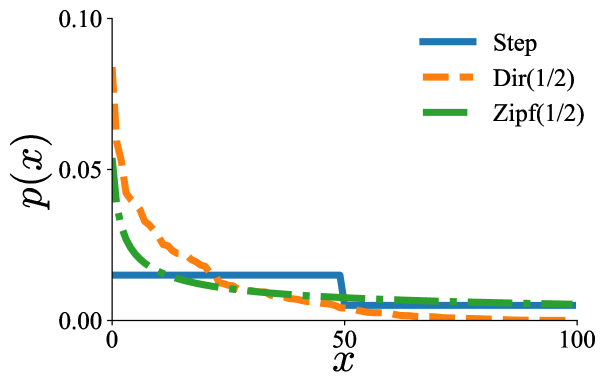
Figure 3: Left: Tail decay of three distributions. Middle: Oracle quantization into $3$ bins: blue, yellow and red. Bin $i$ is given by the set $\{x\,:\,f(p(x)/q(x))\in[T_{i-1},T_{i})\}$. Right: The generator and conjugate generator of $\mathrm{KL}_{\lambda}$ at $\lambda=1/2$.

Before we discuss the bounds in Thm. 1, let us introduce the missing mass problem. This problem was first studied by Good and Turing [21], where the eponymous Good-Turing estimator was proposed to estimate the probability that a new observation drawn from a fixed distribution has never appeared before, in other words, is missing in the current sample; see Fig. 2 (left) for an illustration. The Good-Turing estimator has been widely used in language modeling [33, 12, 11] and studied in theory [41, 48, 47]. An inspiring result coming from this line of work is that the missing mass in a sample of size $n$ concentrates around its expectation [40], which itself decays as $O(k/n)$ when the distribution is supported on $k$ items [3].

There are several merits to Thm. 1. First, (3) holds for any distributions with a countable support. Second, it does not depend on $p_{*}$ and is adapted to the tail behavior of $P$ and $Q$. For instance, if $P$ is defined as $P(a)\propto a^{-2}$ for $a\in[k]$, then $\alpha_{n}(P)\propto(\log{k})/\sqrt{n}$, which is much better than $\sqrt{k/n}$ in (4) in terms of the dependency on $k$. This phenomenon is also demonstrated empirically in Sec. 5. Third, it captures a parametric rate of convergence, i.e., $O(n^{-1/2})$, up to a logarithmic factor. In fact, this rate is not improvable in a related problem of estimating $\mathrm{KL}(P\|Q)$, even with the assumption that $P/Q$ is bounded [7]. The bound in (4) is a distribution-free bound, assuming $k$ is finite. Note that it also gives an upper bound on the sample complexity by setting the right hand side of (5) to be $\epsilon$ and solve for $n$, this is roughly $O((\sqrt{\log{1/\delta}}+\sqrt{k})^{2}/\epsilon^{2})$.

The proof of Thm. 1 relies on two new results: (a) a concentration bound around $\mathbb{E}[{\operatorname{FI}}(\hat{P}_{n},\hat{Q}_{n})]$, which can be obtained by McDiarmid’s inequality, and (b) an upper bound for the statistical error, i.e., $\mathbb{E}\big{|}{\operatorname{FI}}(\hat{P}_{n},\hat{Q}_{n})-{\operatorname{FI}}(P,Q)\big{|}$, which is upper bounded by

$$O\left([\alpha_{n}(P)+\alpha_{n}(Q)]\log{n}+\beta_{n}(P)+\beta_{n}(Q)\right)\leq O\big{(}(\sqrt{k/n}+k/n)\log{n}\big{)}\,.$$ (5)

The concentration bound gives the term $\sqrt{n^{-1}\log{1/\delta}}$. The statistical error bound is achieved by splitting the masses of $P$ and $Q$ into two parts: one that appears in the sample and one that never appears. The first part can be controlled by a Lipschitz-like property of the frontier integral, leading to the term $\alpha_{n}(P)+\alpha_{n}(Q)$, and the second part, $\beta_{n}(P)+\beta_{n}(Q)$, falls into the missing mass framework. In addition, the rate $k/n$ for $\beta_{n}$ shown here matches the rate for the missing mass.

Statistical consistency of the divergence frontiers. While Thm. 1 establishes the consistency of the frontier integral, it is also of great interest to know whether the divergence frontier itself can be consistently estimated. In fact, similar bounds hold for the worst-case error of $\mathcal{F}(\hat{P}_{n},\hat{Q}_{n})$.

Corollary 2.

Under the same assumptions as in Thm. 1, the bounds in (3) and (4) hold for

$$\sup_{\lambda\in[\lambda_{0},1-\lambda_{0}]}\big{\lVert}\big{(}\mathrm{KL}(\hat{P}_{n}\|\hat{R}_{\lambda}),\mathrm{KL}(\hat{Q}_{n}\|\hat{R}_{\lambda})\big{)}-\big{(}\mathrm{KL}(P\|R_{\lambda}),\mathrm{KL}(Q\|R_{\lambda})\big{)}\big{\rVert}_{1},$$

where $\hat{R}_{\lambda}:=\lambda\hat{P}_{n}+(1-\lambda)\hat{Q}_{n}$, with $C$ replaced by $C/\lambda_{0}$ for any $\lambda_{0}\in(0,1)$. In particular, if $\lambda_{0}$ is chosen as $\lambda_{n}=o(1)$ and $\lambda_{n}=\omega(\sqrt{k/n}\log{n})$, then the expected worst-case error above converges to zero at rate $O(\lambda_{n}^{-1}\sqrt{k/n}\log{n})$.

The truncation in Cor. 2 is necessary without imposing additional assumptions, since $\mathrm{KL}(P\|R_{\lambda})$ is close to $\mathrm{KL}(P\|Q)$ for small $\lambda$ and it is known that the minimax quadratic risk of estimating the KL divergence over all distributions with $k$ bins is always infinity [7].

Upper bound for the quantization error. Recall from Sec. 2 that computing the divergence frontiers in practice usually involves a quantization step. Since every quantization will inherently introduce a positive bias in the estimation procedure, it is desirable to control the error, which we call the quantization error, induced by this step. We show that there exists a quantization scheme with error proportional to the inverse of its level. We implement this scheme and empirically verify this rate in Appx. G; certain regimes appear to show even faster convergence.

Let $\mathcal{X}$ be an arbitrary measurable space and $\mathcal{S}$ be a partition of $\mathcal{X}$. The quantization error of $\mathcal{S}$ is the difference $\left\lvert{\operatorname{FI}}(P_{\mathcal{S}},Q_{\mathcal{S}})-{\operatorname{FI}}(P,Q)\right\rvert$. It can be shown that there exists a distribution-dependent partition $\mathcal{S}_{k}$ with level $|\mathcal{S}_{k}|=k$ whose quantization error is no larger than the inverse of its level, i.e.,

$$\left\lvert{\operatorname{FI}}(P,Q)-{\operatorname{FI}}(P_{\mathcal{S}_{k}},Q_{\mathcal{S}_{k}})\right\rvert\leq Ck^{-1}.$$ (6)

The key idea behind the construction of this partition is visualized in Fig. 3 (middle). Combining this bound with the bounds in (5) leads to the following bound for the total estimation error.

Theorem 3.

Assume that $\mathcal{S}_{k}$ is a partition of $\mathcal{X}$ such that $\left\lvert\mathcal{S}_{k}\right\rvert=k\geq 2$. Then the total error $\mathbb{E}\left\lvert{\operatorname{FI}}(\hat{P}_{\mathcal{S}_{k},n},\hat{Q}_{\mathcal{S}_{k},n})-{\operatorname{FI}}(P,Q)\right\rvert$ is upper bounded by

$$C\big{[}\left(\alpha_{n}(P)+\alpha_{n}(Q)\right)\log{n}+\beta_{n}(P)+\beta_{n}(Q)+\left\lvert{\operatorname{FI}}(P,Q)-{\operatorname{FI}}(P_{\mathcal{S}_{k}},Q_{\mathcal{S}_{k}})\right\rvert\big{]}.$$ (7)

Moreover, if the quantization error satisfies the bound in (6), we have

$$\mathbb{E}\left\lvert{\operatorname{FI}}(\hat{P}_{\mathcal{S}_{k},n},\hat{Q}_{\mathcal{S}_{k},n})-{\operatorname{FI}}(P,Q)\right\rvert\leq C\left[\left(\sqrt{k/n}+k/n\right)\log{n}+1/k\right].$$ (8)

Based on the bound in (7), a good choice of $k$ is $\Theta(n^{1/3})$ which balances between the two types of errors. We illustrate in Sec. 5 that this choice works well in practice. This balancing is enabled by the existence of a good quantizer with a distribution-free bound in (6). In practice, this suggests a data-dependent quantizer using nonparametric density estimators. However, directions such as kernel density estimation [42, 26, 28] and nearest-neighbor methods [1] have not met empirical success, as they suffer from the curse of dimensionality common in nonparametric estimation. In particular, [63, 57, 58] propose quantized divergence estimators but only prove asymptotic consistency, and little progress has been made since then. On the other hand, modern data-dependent quantization techniques based on deep neural networks can successfully estimate properties of the density from high dimensional data [53, 23]. Theoretical results for those techniques could complement our analysis. We leverage these powerful methods to scale our approach on real data in Sec. 5.

4 Towards better estimators and interpolated $f$-divergences

Smoothed distribution estimators. When the support size $k$ is large, the statistical performance of the empirical estimator considered in the previous section can be improved. To overcome this challenge, practitioners often use more sophisticated distribution estimators such as the Good-Turing estimator [21, 47] and add-constant estimators [35, 5]. We focus on the add-constant estimator defined below and state here its estimation error when it is applied to estimate the frontier integral from data. Again, this result also holds for the linearized cost $\mathcal{L}_{\lambda}$. We investigate and compare the performance of various distribution estimators in Sec. 5.

For notational simplicity, we assume that $P$ and $Q$ are supported on a common finite alphabet with size $k<\infty$. Note that this is true for the quantized distributions $P_{\mathcal{S}}$ and $Q_{\mathcal{S}}$. For any constant $b>0$, the add-constant estimator of $P$ is defined as $\hat{P}_{n,b}(a)=(N_{a}+b)/(n+kb)$ for each $a\in\mathrm{Supp}(P)$, where $N_{a}=\left\lvert\{i:X_{i}=a\}\right\rvert$ is the number of times $a$ appears in the sample.

Thanks to the smoothing, there is no mass missing in the add-constant estimator. This effect is illustrated for the Krichevsky-Trofimov (add-$1/2$) estimator in Fig. 2. As a result, we can directly utilize the smoothness properties of the frontier integral to get the following bound.

Proposition 4.

Under the same assumptions as in Thm. 3, we have

$$\quad\mathbb{E}\left\lvert{\operatorname{FI}}(\hat{P}_{\mathcal{S}_{k},n,b},\hat{Q}_{\mathcal{S}_{k},n,b})-{\operatorname{FI}}(P,Q)\right\rvert$$

$$\leq C\left[\left(\frac{n(\alpha_{n}(P)+\alpha_{n}(Q))}{n+bk}+\gamma_{n,k}(P)+\gamma_{n,k}(Q)\right)\log{(n/b+k)}+\frac{1}{k}\right],$$ (9)

where $\gamma_{n,k}(P)=(n+bk)^{-1}bk\sum_{a\in\mathcal{X}}\left\lvert P(a)-1/k\right\rvert$. It can be further upper bounded by $\frac{\sqrt{nk}+bk}{n+bk}\log{(n/b+k)}+\frac{1}{k}$ up to a multiplicative constant.

Let us compare the bounds in Prop. 4 with the ones in Thm. 3. For the distribution-dependent bound, the term $\alpha_{n}(P)\log{n}$ in (7) is improved by a factor $n/(n+bk)$ in (4). The missing mass term $\beta_{n}(P)$ is replaced by the total variation distance between $P$ and the uniform distribution on $[k]$ with a factor $bk/(n+bk)$. The improvements in both two terms are most significant when $k/n$ is large. As for the distribution-free bound, when $k/n$ is small, the bound in Prop. 4 scales the same as the one in (8); when $k/n$ is large (i.e., bounded away from $0$ or diverging), it scales as $O(\log{n}+\log{(k/n)}+k^{-1})$ while the one in (8) scales as $O(k\log{n}/n+k^{-1})$. Given the improvement, it would be an interesting venue for future work to consider adaptive estimators in the spirit of [20].

Generalization to $f$-divergences. Estimation of the $\chi^{2}$ divergence is useful for variational inference [17] and GAN training [39, 61]. More generally, estimating $f$-divergences from samples is a fundamental problem in machine learning and statistics [45, 29, 10, 52]. We extend our previous results to estimating general $f$-divergences (which satisfy some regularity assumptions) using the same two-step procedure of quantization and estimation of multinomial distributions from samples.

We start by reviewing the definition of $f$-divergences. Let $f:(0,\infty)\rightarrow\mathbb{R}$ be a nonnegative and convex function with $f(1)=0$. Let $P,Q\in\mathcal{P}(\mathcal{X})$ be dominated by some measure $\mu\in\mathcal{P}(\mathcal{X})$ with densities $p$ and $q$, respectively. The $f$-divergence generated by $f$ is defined as

$$D_{f}(P\|Q)=\int_{\mathcal{X}}q(x)f\left(\frac{p(x)}{q(x)}\right)\mathrm{d}\mu(x)\,,$$

with the convention that $f(0)=f(0^{+})$ and $0f(p/0)=pf^{*}(0)$, where $f^{*}(0)=f^{*}(0^{+})\in[0,\infty]$ for $f^{*}(t)=tf(1/t)$. We call $f^{*}$ the conjugate generator to $f$. An illustration of the generator to $\mathrm{KL}_{1/2}$ can be found in Fig. 3 (right). Note that the conjugacy here is unrelated to the convex conjugacy but is based on the perspective transform. The function $f^{*}$ also generates an $f$-divergence, which is referred to as the conjugate divergence to $D_{f}$ since $D_{f^{*}}(P\|Q)=D_{f}(Q\|P)$.

The quantization error bound (6) holds for all $f$-divergences which are bounded, i.e., $f(0)+f^{*}(0)<\infty$. The high probability bounds in Thm. 1 also hold for $f$-divergences, under some regularity assumptions: (a) $\left\lvert f^{\prime}(t)\right\rvert\propto\log{t^{-1}}$ and $\left\lvert(f^{*})^{\prime}(t)\right\rvert\propto\log{t^{-1}}$ for small $t$, which guarantees that $f$ is approximately Lipschitz and cannot vary too fast; (b) $tf^{\prime\prime}(t)$ and $t(f^{*})^{\prime\prime}(t)$ are bounded, which is a technical assumption that helps control the variation of $f$ around zero. The interpolated $\chi^{2}$ divergence, defined analogously as the interpolated KL divergence, satisfies these conditions.

In the Appendix, we prove all the results for general $f$-divergences and show that both the frontier integral and the linearized cost are $f$-divergences satisfying the regularity conditions, recovering Thm. 1 and Thm. 3 as special cases.

5 Experiments

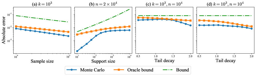
Figure 4: Statistical error of the estimated frontier integral on synthetic data. (a): Zipf$(2)$ and Zipf$(2)$ with $k=10^{3}$; (b): Zipf$(2)$ and Zipf$(2)$ with $n=2\times 10^{4}$; (c): $\mathrm{Dir}(\mathbf{1})$ and Zipf$(r)$ with $k=10^{3}$ and $n=10^{4}$; (d): $\mathrm{Zipf}(2)$ and $\mathrm{Zipf}(r)$ with $k=10^{3}$ and $n=10^{4}$. The bounds are scaled by $100$.

We investigate the empirical behavior of the divergence frontier and the frontier integral on both synthetic and real data. Our main findings are: (a) the statistical error bound approximately reveals the rate of convergence of the empirical estimator; (b) the smoothed distribution estimators improve the estimation accuracy; (c) the quantization level suggested by the theory works well empirically. The results for the divergence frontier and the frontier integral are almost identical. We focus on the latter here due to space constraints. In all the plots, we visualize the average absolute error computed from 100 repetitions with shaded region denoting one standard deviation around the mean. More details and additional results, including the ones for the divergence frontier, are deferred to Appx. G. The code to reproduce the experiments is available online.

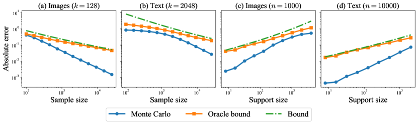
Figure 5: Statistical error of the estimated frontier integral on real data. (a): Image data (CIFAR-10) with $k=128$; (b): Text data (WikiText-103) with $k=2048$; (c): Image data (CIFAR-10) with $n=1000$; (d): Text data (WikiText-103) with $n=10000$. The bounds are scaled by $30$.

5.1 Experimental setup

We work with synthetic data in the case when $k=\left\lvert\mathcal{X}\right\rvert<\infty$ as well as real image and text data.

Synthetic Data. Following the experimental settings in [47], we consider three types of distributions: (a) the Zipf$(r)$ distribution with $r\in\{0,1,2\}$ where $P(i)\propto i^{-r}$. Note that Zipf$(r)$ is regularly varying with index $-r$; see, e.g., [56, Appx. B]. (b) the Step distribution where $P(i)=1/2$ for the first half bins and $P(i)=3/2$ for the second half bins. (c) the Dirichlet distribution $\mathrm{Dir}(\alpha)$ with $\alpha\in\{\mathbf{1}/2,\mathbf{1}\}$; see Fig. 1 (left) for an illustration. In total, there are 6 different distributions, giving $21$ different pairs of $(P,Q)$. For each pair $(P,Q)$, we generate i.i.d. samples of size $n$ from each of them, and estimate the divergence frontier as well as the frontier integral from these samples.

Real Data. We consider two domains: images and text. For the image domain, we train a StyleGAN2 [32] on the CIFAR-10 dataset [36] using the publicly available code with default hyperparameters. To evaluate the divergence frontiers, we use the test set of 10k images as the target distribution $P$ and we sample 10k images from the generative model as the model distribution $Q$. For the text domain, we fine-tune a pretrained GPT-2 [50] model with 124M parameters (i.e., GPT-2 small) on the Wikitext-103 dataset [43]. We use the open-source HuggingFace Transformers library [65] for training, and generate 10k 500-token completions using top-$p$ sampling and 100-token prefixes.

We take the following steps to compute the frontier integral. First, we represent each image/text by its features [27, 54, 37]. Second, we learn a low-dimensional feature embedding which maintains the neighborhood structure of the data while encouraging the features to be uniformly distributed on the unit sphere [53]. Third, we quantize these embeddings on a uniform lattice with $k$ bins. For each support size $k$, this gives us quantized distributions $P_{\mathcal{S}_{k}}$ and $Q_{\mathcal{S}_{k}}$. Finally, we sample $n$ i.i.d. observations from each of these distributions and consider the empirical distributions $\hat{P}_{\mathcal{S}_{k},n}$ and $\hat{Q}_{\mathcal{S}_{k},n}$ as well as the smoothed distribution estimators computed from these samples.

Performance Metric. We are interested in the estimation of the frontier integral ${\operatorname{FI}}(P,Q)$ using estimators ${\operatorname{FI}}(\hat{P}_{n},\hat{Q}_{n})$ for the empirical estimator as well as the smoothed distribution estimator. We measure the quality of estimation using the absolute error, which is defined as $\lvert{\operatorname{FI}}(\hat{P}_{n},\hat{Q}_{n})-{\operatorname{FI}}(P,Q)\rvert$. For the real data, we measure the error of estimating ${\operatorname{FI}}(P_{\mathcal{S}_{k}},Q_{\mathcal{S}_{k}})$ by ${\operatorname{FI}}(\hat{P}_{\mathcal{S}_{k},n},\hat{Q}_{\mathcal{S}_{k},n})$.

5.2 Tightness of the Statistical Bound

We investigate the tightness of the statistical error bound of Thm. 1 with respect to the sample size $n$ and the support size $k$, in order to verify the validity of the theory in practically relevant settings.

We estimate the expected absolute error $\mathbb{E}|{\operatorname{FI}}(\hat{P}_{n},\hat{Q}_{n})-{\operatorname{FI}}(P,Q)|$ from a Monte Carlo estimate using $100$ random trials. We compare it with the following bounds in Thm. 1:

1. Bound: the distribution independent bound $(\sqrt{k/n}+k/n)\log n$.

2. Oracle Bound: the distribution dependent bound $\left(\alpha_{n}(P)+\alpha_{n}(Q)\right)\log n+\beta_{n}(P)+\beta_{n}(Q)$. We assume that the quantities $\alpha_{n}$ and $\beta_{n}$ defined in Thm. 1 are known.

We fix $k$, plot each of these quantities in a log-log plot with varying $n$ and compare their slopes. We then repeat the experiment with $n$ fixed and $k$ varying. We often scale the bounds by a constant for easier visual comparison of the slopes; this only changes the intercept and leaves the slope unchanged.

Thm. 1 is tight for synthetic data. Fig. 4 gives the Monte Carlo estimate and the bounds of the statistical error for various synthetic data distributions. In Fig. 4(a), we observe that the bound has approximately the same slope as the Monte Carlo estimate, while the oracle bound has a slightly worse slope. In Fig. 4(b), we observe that the oracle bound captures the correct rate for $k>300$, while the distribution-independent bound captures the correct rate at small $k$. For the right two plots, both bounds capture the right rate over a wide range of tail decay. The oracle bound is tighter for fast decay, where the distribution-independent bounds on $\alpha_{n}(Q)$ and $\beta_{n}(Q)$ can be very pessimistic.

Thm. 1 is somewhat tight for real data. Fig. 5 contains the analogous plot for real data, where the observations are similar. In Fig. 5(b), we see that the oracle bound captures the right rate for small sample sizes where $k/n>1$. However, for large $n$, the distribution-independent bound is better at matching the slope of the Monte Carlo estimate. The same is true for Fig. 5(c), where the oracle bound is better for large $k$. For parts (a) and (d), however, both bounds do not capture the right slope of the Monte Carlo estimate; Thm. 1 is not a tight upper bound in this case.

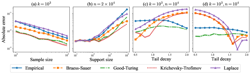
Figure 6: Statistical error with smoothed distribution estimators on synthetic data. (a): $\mathrm{Zipf}(0)$ and $\mathrm{Dir}(\mathbf{1}/2)$ with $k=10^{3}$; (b): $\mathrm{Zipf}(0)$ and $\mathrm{Dir}(\mathbf{1}/2)$ with $n=2\times 10^{4}$; (c): $\mathrm{Dir}(\mathbf{1})$ and $\mathrm{Zipf}(r)$ with $k=10^{3}$ and $n=10^{4}$; (d): $\mathrm{Zipf}(2)$ and $\mathrm{Zipf}(r)$ with $k=10^{3}$ and $n=10^{4}$.

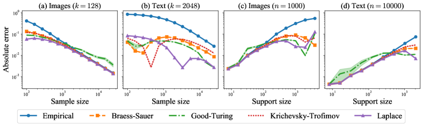
Figure 7: Statistical error with smoothed distribution estimators on real data. (a): Image data (CIFAR-10) with $k=128$; (b): Text data (WikiText-103) with $k=2048$; (c): Image data (CIFAR-10) with $n=1000$; (d): Text data (WikiText-103) with $n=10000$. The bounds are scaled by $15$.

5.3 Effect of Smoothed Distribution Estimators

We now show that smoothed estimators can lead to improved estimation over the naïve empirical estimator and thus improved sample complexity as shown in Prop. 4. This is practically significant in the context of generative models, since one can have an equally good estimate of the divergence frontier with fewer samples using smoothed estimators [54, 18].

Concretely, we compare the Monte Carlo estimates of the absolute error $\mathbb{E}|{\operatorname{FI}}(\hat{P}_{n},\hat{Q}_{n})-{\operatorname{FI}}(P,Q)|$ for the plug-in estimate (denoted “Empirical”) with the corresponding estimates for smoothed estimators. We consider 4 smoothed estimators as in [47]: the (modified) Good-Turing estimator, as well as three add-constant estimators: the Laplace, Krichevsky-Trofimov and Braess-Sauer estimators.

Smoothed estimators are more efficient than the empirical estimator. We compare the smoothed estimators to the empirical one in Fig. 6 on synthetic data and Fig. 7 on real data. In general, the smoothed distribution estimators reduces the absolute error. For parts (a) and (b) of Fig. 6, the Good-Turing and the Krichevsky-Trofimov estimators have the best absolute error. For parts (c) and (d), the Good-Turing estimator is adapted to various regimes of tail-decay, outperforming the empirical estimator. The Krichevsky-Trofimov and Braess-Sauer estimators, on the other hand, exhibit small absolute error for particular decay regimes. The results are similar for real data in Fig. 7.

Practical guidance on choosing a smoothed estimator. While the smoothed estimators offer a marked improvement when $k/n$ is large (that is, close to 1), the best estimator is problem-dependent. As a rule of thumb, we suggest the Krichevsky-Trofimov estimator which works well in the large $k/n$ regime but is still competitive when $k/n$ is small (i.e., large $n$).

5.4 Quantization Error

Next, we study the effect of the quantization level $k$ on the total error. We consider a simple $2$-dimensional synthetic setting where the distributions $P,Q$ are either the multivariate normal or $t$-distributions. We use data-driven quantization with $k$-means to obtain a quantization $\mathcal{S}_{k}$: each component of the partition is the region corresponding to one cluster. Finally, we plot the absolute error $\mathbb{E}|{\operatorname{FI}}(P,Q)-{\operatorname{FI}}(\hat{P}_{\mathcal{S}_{k},n},\hat{Q}_{\mathcal{S}_{k},n})|$, where the ${\operatorname{FI}}(P,Q)$ is computed using numerical integration and the expectation is estimated with Monte Carlo simulations.

The choice $k=\Theta(n^{1/3})$ works the best. We compare $k=n^{1/r}$ for $r=2,3,4,5$ in Fig. 8. For small $n$, $r\geq 3$ all perform similarly, but $r=3$ clearly outperforms other choices for $n\geq 10^{4}$. While our theory does not directly apply for data-dependent partitioning schemes, the choice $k=\Theta(n^{1/3})$ suggested by Thm. 3 nevertheless works well in practice.

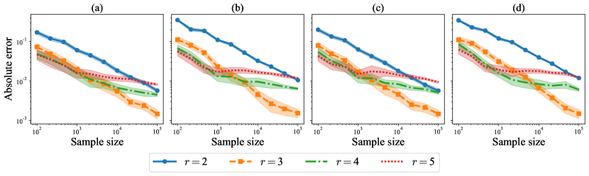
Figure 8: Total error with quantization level $k\propto n^{1/r}$ on 2-dimensional continuous data. (a): $\mathcal{N}(0,I_{2})$ and $\mathcal{N}(1,I_{2})$; (b): $\mathcal{N}(0,I_{2})$ and $\mathcal{N}(0,5I_{2})$; (c): $t_{4}(0,I_{2})$ and $t_{4}(1,I_{2})$ (multivariate t-distribution with 4 degrees of freedom); (d): $t_{4}(0,I_{2})$ and $t_{4}(0,5I_{2})$.

6 Conclusion

In this paper, we study the statistical behavior of the divergence frontiers and the proposed integral summary estimated from data. We decompose the estimation error into two components, the statistical error and the quantization error, to conform with the approximation procedure commonly used in practice. We establish non-asymptotic bounds on both of the two errors. Our bounds shed light on the optimal choice of the quantization level $k$—they suggests that the two errors can be balanced at $k=\Theta(n^{1/3})$. We also derive a new concentration inequality for the frontier integral, which provides the sample complexity of achieving a small error in high probability. Finally, we demonstrate both theoretically and empirically that the use of smoothed distribution estimators can improve the estimation accuracy. All the results can be generalized to a large class of interpolation-based $f$-divergences. Provided new theoretical results on modern data-dependent quantization schemes using deep neural networks, it would be an interesting direction for future work to specialize our bounds to such quantization schemes. Extending our results to $\beta$-divergences could also be interesting.

Acknowledgments.

The authors would like to thank J. Thickstun for fruitful discussions. Part of this work was done while Z. Harchaoui was visiting the Simons Institute for the Theory of Computing. This work was supported by NSF DMS-2134012, NSF CCF-2019844, the CIFAR program “Learning in Machines and Brains”, and faculty research awards.

Appendix

Appendix A $f$-divergence: review and examples

We review the definition of $f$-divergences and give a few examples.

Let $f:(0,\infty)\to\mathbb{R}$ be a convex function with $f(1)=0$. Let $P,Q\in\mathcal{P}(\mathcal{X})$ be dominated by some measure $\mu\in\mathcal{P}(\mathcal{X})$ with densities $p$ and $q$, respectively. The $f$-divergence generated by $f$ is

$$D_{f}(P\|Q)=\int_{\mathcal{X}}q(x)f\left(\frac{p(x)}{q(x)}\right)\mathrm{d}\mu(x)\,,$$

with the convention that $f(0):=\lim_{t\to 0^{+}}f(t)$ and $0f(p/0)=pf^{*}(0)$, where $f^{*}(0)=\lim_{x\rightarrow 0^{+}}xf(1/x)\in[0,\infty]$. Hence, $D_{f}(P\|Q)$ can be rewritten as

$$D_{f}(P\|Q)=\int_{q>0}q(x)f\left(\frac{p(x)}{q(x)}\right)\mathrm{d}\mu(x)+f^{*}(0)P[q=0]\,,$$

with the agreement that the last term is zero if $P[q=0]=0$ no matter what value $f^{*}(0)$ takes (which could be infinity). For any $c\in\mathbb{R}$, it holds that $D_{f_{c}}(P\|Q)=D_{f}(P\|Q)$ where $f_{c}(t)=f(t)+c(t-1)$. Hence, we also assume, w.l.o.g., that $f(t)\geq 0$ for all $t\in(0,\infty)$. To summarize, $f$ is convex and nonnegative with $f(1)=0$. As a result, $f$ is non-increasing on $(0,1]$ and non-decreasing on $[1,\infty)$.

The conjugate generator to $f$ is the function $f^{*}:(0,\infty)\to[0,\infty)$ defined by

$$f^{*}(t)=tf(1/t)\,,$$

where again we define $f^{*}(0)=\lim_{t\to 0^{+}}f^{*}(t)$. Since $f^{*}$ can be constructed by the perspective transform of $f$, it is also convex. We can verify that $f^{*}(1)=0$ and $f^{*}(t)\geq 0$ for all $t\in(0,\infty)$, so it defines another divergence $D_{f^{*}}$. We call this the conjugate divergence to $D_{f}$ since

$$D_{f^{*}}(P\|Q)=D_{f}(Q\|P)\,.$$

The divergence $D_{f}$ is symmetric if and only if $f=f^{*}$, and we write it as $D_{f}(P,Q)$ to emphasize the symmetry.

Example 5.

We illustrate a number of examples.

1. KL divergence: It is an $f$-divergence generated by $f_{\mathrm{KL}}(t)=t\log t-t+1$.

2. Interpolated KL divergence: For $\lambda\in(0,1)$, the interpolated KL divergence is defined as

   $$\mathrm{KL}_{\lambda}(P\|Q)=\mathrm{KL}(P\|\lambda P+(1-\lambda)Q)\,,$$

   which is a $f$-divergence generated by

   $$f_{\mathrm{KL},\lambda}(t)=t\log\left(\frac{t}{\lambda t+1-\lambda}\right)-(1-\lambda)(t-1)\,.$$

3. Jensen-Shannon divergence: The Jensen-Shannon Divergence is defined as

   $$D_{\mathrm{JS}}(P,Q)=\frac{1}{2}\mathrm{KL}_{1/2}(P\|Q)+\frac{1}{2}\mathrm{KL}_{1/2}(Q\|P).$$

   More generally, we have the $\lambda$-skew Jensen-Shannon Divergence [46], which is defined for $\lambda\in(0,1)$ as $D_{\mathrm{JS},\lambda}=\lambda\mathrm{KL}_{\lambda}(P\|Q)+(1-\lambda)\mathrm{KL}_{1-\lambda}(Q\|P)$. This is an $f$-divergence generated by

   $$f_{\mathrm{JS},\lambda}(t)=\lambda t\log\left(\frac{t}{\lambda t+1-\lambda}\right)+(1-\lambda)\log\left(\frac{1}{\lambda t+1-\lambda}\right)\,.$$

   Note that this is the linearized cost defined in (1)

4. Frontier Integral: From Prop. 6, ${\operatorname{FI}}$ is an $f$-divergence generated by

   $$f_{\operatorname{FI}}(t)=\frac{t+1}{2}-\frac{t}{t-1}\log t\,.$$

5. Interpolated $\chi^{2}$ divergence: Similar to the interpolated KL divergence, we can define the interpolated $\chi^{2}$ divergence $D_{\chi^{2},\lambda}$ and the corresponding convex generator $f_{\chi^{2},\lambda}$ for $\lambda\in(0,1)$ as

   $$D_{\chi^{2},\lambda}(P\|Q)=D_{\chi^{2}}(P\|\lambda P+(1-\lambda)Q)\,,\quad\text{and,}\quad f_{\chi^{2},\lambda}(t)=\frac{(t-1)^{2}}{\lambda t+1-\lambda}\,.$$

   The usual Neyman and Pearson $\chi^{2}$ divergences are respectively obtained in the limits $\lambda\to 1$ and $\lambda\to 0$.

6. Squared Le Cam distance: The squared Le Cam distance is, up to scaling, a special case of the interpolated $\chi^{2}$ divergence with $\lambda=1/2$:

   $$D_{\mathrm{LC}}(P,Q)=\frac{1}{4}D_{\chi^{2},1/2}(P\|Q)\,.$$

7. Squared Hellinger Distance: It is an $f$-divergence generated by $f_{H}(t)=(1-\sqrt{t})^{2}$.

Appendix B Properties of the frontier integral

We prove some properties of the frontier integral here.

First, the frontier integral can be computed in closed form as below.

Proposition 6.

Let $P$ and $Q$ be dominated by some probability measure $\mu$ with density $p$ and $q$, respectively. Then,

$${\operatorname{FI}}(P,Q)=\int_{\mathcal{X}}\mathbbm{1}{\{p(x)\neq q(x)\}}\left(\frac{p(x)+q(x)}{2}-\frac{p(x)q(x)}{p(x)-q(x)}\log\frac{p(x)}{q(x)}\right)\mathrm{d}\mu(x)\,,$$ (10)

with the convention $0\log 0=0$. Moreover, ${\operatorname{FI}}$ is an $f$-divergence generated by the convex function

$$f_{{\operatorname{FI}}}(t)=\frac{t+1}{2}-\frac{t}{t-1}\log t\,,$$

with the understanding that $f_{{\operatorname{FI}}}(1)=\lim_{t\to 1}f_{{\operatorname{FI}}}(t)=0$.

Proof of Prop. 6.

Let $\bar{\lambda}=1-\lambda$. By Tonelli’s theorem, it holds that ${\operatorname{FI}}(P,Q)=2\int_{\mathcal{X}}h(p(x),q(x))\mathrm{d}\mu(x)$, where

$$h(p,q)=\int_{0}^{1}\left(\lambda p\log p+\bar{\lambda}q\log q-(\lambda p+\bar{\lambda}q)\log(\lambda p+\bar{\lambda}q)\right)\mathrm{d}\lambda.$$

When $p=q$, the integrand is $0$. If $q=0$, then the second term inside the integral is $0$, while the first term is

$$\int_{0}^{1}\lambda p\log\frac{1}{\lambda}\mathrm{d}\lambda=\frac{p}{4}\,.$$

Finally, when $p\neq q$ are both non-zero, we evaluate the integral to get,

$$h(p,q)=\frac{p}{2}\log p+\frac{q}{2}\log q-\frac{2p^{2}\log p-p^{2}-2q^{2}\log q+q^{2}}{4(p-q)}\,,$$

and rearranging the expression completes the proof. ∎

Next, the frontier integral is symmetric and bounded.

Proposition 7.

The frontier integral satisfies the following properties:

1. ${\operatorname{FI}}(P,Q)={\operatorname{FI}}(Q,P)$.

2. $0\leq{\operatorname{FI}}(P,Q)\leq 1$ with ${\operatorname{FI}}(P,Q)=0$ if and only if $P=Q$.

Proof of Prop. 7.

The first part follows from the closed form expression in Prop. 6. For the second part, we get the upper bound as

$${\operatorname{FI}}(P,Q)\leq\int_{\mathcal{X}}\frac{p(x)+q(x)}{2}\mathrm{d}\mu(x)=1\,.$$

We have ${\operatorname{FI}}(P,Q)\geq 0$ with ${\operatorname{FI}}(P,P)=0$ since ${\operatorname{FI}}$ is an $f$-divergence. Further, since $f_{{\operatorname{FI}}}$ is strictly convex at $1$, we get that ${\operatorname{FI}}(P,Q)=0$ only if $P=Q$.∎

Appendix C Regularity assumptions

In this section, we state and discuss the regularity assumptions required for the statistical error bounds. Throughout, we assume that $\mathcal{X}$ is a finite set (for instance, on the quantized space). We upper bound the expected error of the empirical $f$-divergences estimated from data.

We use the convention that all higher order derivatives of $f$ and $f^{*}$ at $0$ are defined as the corresponding limits as $x\to 0^{+}$ (if they exist). Further, we use the notation

$$\psi(p,q) =qf(p/q)=pf^{*}(q/p),$$ (11)

so that $D_{f}(P\|Q)=\sum_{a\in\mathcal{X}}\psi(P(a),Q(a))$.

C.1 Assumptions

We make the following assumptions about the functions $f$ and $f^{*}$.

Assumption 8.

The generator $f$ is twice continuously differentiable with $f^{\prime}(1)=0$. Moreover,

1. We have $C_{0}:=f(0)<\infty$ and $C_{0}^{*}:=f^{*}(0)<\infty$.

2. There exist constants $C_{1},C_{1}^{*}<\infty$ such that for every $x\in(0,1)$, we have,

   $$|f^{\prime}(t)| \leq C_{1}\left(1\vee\log{1}/{t}\right),\quad\text{and},\quad|(f^{*})^{\prime}(t)|\leq C_{1}^{*}\left(1\vee\log{1}/{t}\right)\,.$$

3. There exist constants $C_{2},C_{2}^{*}<\infty$ such that for every $t\in(0,\infty)$, we have,

   $$\frac{t}{2}f^{\prime\prime}(t) \leq C_{2}\,,\quad\text{and},\quad\frac{t}{2}(f^{*})^{\prime\prime}(t)\leq C_{2}^{*}\,.$$

Remark 9.

We discuss the asymptotics of the assumptions.

1. Assumption (A1) ensures boundedness of the $f$-divergence. Indeed, $f(0)=\infty$ leads to $D_{f}(P\|Q)=\infty$ if there exists an atom $a\in\mathcal{X}$ such that $P(a)=0$ but $Q(a)\neq 0$. This happens, for instance, with the reverse KL divergence ($f(t)=-\log t+t-1$). By symmetry, $f^{*}(0)=\infty$ leads to a case where $D_{f}(P\|Q)=\infty$ if there exists an atom $a\in\mathcal{X}$ such that $Q(a)=0$ but $P(a)\neq 0$, as in the (forward) KL divergence.

2. Since $f^{\prime}$ is monotonic nondecreasing and $f^{\prime}(1)=0$, we have that $f^{\prime}(0)\leq 0$ (with strict inequality if $f$ is strictly convex at $1$). In fact, $f^{\prime}(0)=-\infty$ for each of the divergences considered in Example 5. Assumption (A2) requires $f^{\prime}(t)$ to behave as $\log{1/t}$ when $t\to 0$. Likewise for $(f^{*})^{\prime}$.

3. Likewise, we have that $f^{\prime\prime}(0)=\infty$ and $f^{\prime\prime}(\infty)=0$ for each of the divergence considered in Example 5. However, Assumption (A3) makes assumptions on the rates of these limits. Namely, $f^{\prime\prime}$ should diverge no faster than $1/t$ as $t\to 0$ and $f^{\prime\prime}$ should converge to $0$ at least as fast as $1/t^{2}$ as $t\to\infty$. We can summarize the implied asymptotics of $f^{\prime\prime}$ as

   $$f^{\prime\prime}(t)=\begin{cases}\Omega(1/t)\,,&\text{ if }t\to 0\,,\\ O(1/t^{2})\,,&\text{ if }t\to\infty\,.\end{cases}$$

C.2 Examples satisfying the assumptions

We now consider the examples in Example 5. The constants are summarized in Tab. 1.

Table 1: Examples of $f$-divergences and whether they satisfy Assumptions (A1)-(A3). Here, $\lambda\in(0,1)$ is a parameter of the interpolated or skew divergences, and we define $\bar{\lambda}:=1-\lambda$.

$f$-divergence	Satisfies Assumptions?	$C_{0}$	$C_{0}^{*}$	$C_{1}$	$C_{1}^{*}$	$C_{2}$	$C_{2}^{*}$
KL	No	$1$	$\infty$
Interpolated KL	Yes	$\bar{\lambda}$	$\log\tfrac{1}{\lambda}-\bar{\lambda}$	$1$	$\tfrac{\bar{\lambda}^{2}}{\lambda}$	$\tfrac{1}{2}$	$\tfrac{\bar{\lambda}}{8\lambda}$
JS	Yes	$\tfrac{1}{2}\log 2$	$\tfrac{1}{2}\log 2$	$\tfrac{1}{2}$	$\tfrac{1}{2}$	$\tfrac{1}{4}$	$\tfrac{1}{4}$
Skew JS	Yes	$\bar{\lambda}\log\tfrac{1}{\bar{\lambda}}$	$\lambda\log\tfrac{1}{\lambda}$	$\lambda$	$\bar{\lambda}$	$\tfrac{\lambda}{2}$	$\tfrac{\bar{\lambda}}{2}$
Frontier integral	Yes	$\tfrac{1}{2}$	$\tfrac{1}{2}$	$4$	$4$	$\tfrac{1}{2}$	$\tfrac{1}{2}$
LeCam	Yes	$\tfrac{1}{2}$	$\tfrac{1}{2}$	$2$	$2$	$\tfrac{8}{27}$	$\tfrac{8}{27}$
Interpolated $\chi^{2}$	Yes	$\tfrac{1}{\bar{\lambda}}$	$\tfrac{1}{\lambda}$	$\tfrac{2}{\bar{\lambda}^{2}}$	$\tfrac{2}{\lambda^{2}}$	$\frac{4}{27\lambda\bar{\lambda}^{2}}$	$\tfrac{4}{27\lambda^{2}\bar{\lambda}}$
Hellinger	No	$1$	$1$	$\infty$	$\infty$

KL divergence. We have

$$f_{\mathrm{KL}}(t)=t\log t-t+1\,\quad\text{and}\quad f^{*}_{\mathrm{KL}}(t)=-\log t+t-1\,.$$

We have $f(0)=1$ but $f^{*}(0)=\infty$. Therefore, the KL divergence does not satisfy our assumptions. Indeed, this is because the KL divergence can be unbounded.

Interpolated KL Divergence. Let $\lambda\in(0,1)$ be a parameter and denote $\bar{\lambda}=1-\lambda$. We have

$$f_{\mathrm{KL},\lambda}(t)=t\log\left(\frac{t}{\lambda t+\bar{\lambda}}\right)-\bar{\lambda}(t-1)\quad\text{and}\quad f^{*}_{\mathrm{KL},\lambda}(t)=-\log(\bar{\lambda}t+\lambda)+\bar{\lambda}(t-1)\,.$$

The corresponding derivatives are

$$f_{\mathrm{KL},\lambda}^{\prime}(t)=\frac{\bar{\lambda}}{\lambda t+\bar{\lambda}}+\log\left(\frac{t}{\lambda t+\bar{\lambda}}\right)-\bar{\lambda},\quad \quad(f^{*}_{\mathrm{KL},\lambda})^{\prime}(t)=\bar{\lambda}-\frac{\bar{\lambda}}{\bar{\lambda}t+\lambda},$$

$$f_{\mathrm{KL},\lambda}^{\prime\prime}(t)=\frac{\bar{\lambda}^{2}}{t(\lambda t+\bar{\lambda})^{2}},\quad \quad(f^{*}_{\mathrm{KL},\lambda})^{\prime\prime}(t)=\frac{\bar{\lambda}^{2}}{(\bar{\lambda}t+\lambda)^{2}}\,.$$

Proposition 10.

The interpolated KL divergence generated by $f_{\mathrm{KL},\lambda}$ satisfies 8 with

$$C_{0}=1-\lambda,\quad C_{0}^{*}=\log\frac{1}{\lambda}-1+\lambda,\quad C_{1}=1,\quad C_{1}^{*}=\frac{(1-\lambda)^{2}}{\lambda},\quad C_{2}=\frac{1}{2},\quad C_{2}^{*}=\frac{1-\lambda}{8\lambda}\,.$$

Proof.

First, $C_{0},C_{0}^{*}$ can be computed directly. Second, it is clear that

$$-f_{\mathrm{KL},\lambda}^{\prime}(t)=\log\frac{1}{t}+\log(\lambda t+\bar{\lambda})-\frac{\bar{\lambda}}{\lambda t+\bar{\lambda}}+\bar{\lambda}\leq\log\frac{1}{t}+\log{1}-\bar{\lambda}+\bar{\lambda}=\log{\frac{1}{t}}\,$$

for all $x\in(0,1)$. Moreover, since $f$ is convex and $f^{\prime}_{\mathrm{KL},\lambda}(1)=0$, it holds that $f^{\prime}_{\mathrm{KL},\lambda}(x)\leq 0$ for all $x\in(0,1)$, and thus $C_{1}=1$. Next, we note that $|(f^{*}_{\mathrm{KL},\lambda})^{\prime}(x)|\leq{\bar{\lambda}^{2}}/{\lambda}$ holds uniformly on $(0,1)$ (or equivalently that $f^{*}_{\mathrm{KL},\lambda}$ is Lipschitz); this gives $C_{1}^{*}$. Next, we have

$$C_{2}=\sup_{t>0}\left\{\frac{1}{2}tf_{\mathrm{KL},\lambda}^{\prime\prime}(t)\right\}\leq\frac{1}{2}\,,$$

since the function inside the sup is monotonic decreasing on $(0,\infty)$. Finally, we have

$$C_{2}^{*}=\sup_{t>0}\left\{\frac{1}{2}t(f^{*}_{\mathrm{KL},\lambda})^{\prime\prime}(t)\right\}=\frac{\bar{\lambda}}{8\lambda}\,,$$

since the term inside the sup is maximized at $t=\lambda/\bar{\lambda}$. ∎

Skew Jensen-Shannon Divergence. Let $\lambda\in(0,1)$ be a parameter and $\bar{\lambda}=1-\lambda$. We have,

$$f_{\mathrm{JS},\lambda}(t)=\lambda t\log\left(\frac{t}{\lambda t+\bar{\lambda}}\right)+\bar{\lambda}\log\left(\frac{1}{\lambda t+\bar{\lambda}}\right)=f^{*}_{\mathrm{JS},1-\lambda}(t)\,.$$

Its derivatives are

$$f_{\mathrm{JS},\lambda}^{\prime}(t)=\lambda\log\left(\frac{t}{\lambda t+\bar{\lambda}}\right)\,\quad\mbox{and}\quad f_{\mathrm{JS},\lambda}^{\prime\prime}(t)=\frac{\lambda\bar{\lambda}}{t(\lambda t+\bar{\lambda})}\,.$$

Proposition 11.

The $\lambda$-skew JS divergence generated by $f_{\mathrm{JS},\lambda}$ above satisfies 8 with

$$C_{0}=(1-\lambda)\log\frac{1}{1-\lambda},\quad C_{0}^{*}=\lambda\log\frac{1}{\lambda},\quad C_{1}=\lambda,\quad C_{1}^{*}=1-\lambda,\quad C_{2}=\frac{\lambda}{2},\quad C_{2}^{*}=\frac{1-\lambda}{2}\,.$$

Proof.

For $C_{1}$, we have

$$-f_{\mathrm{JS},\lambda}^{\prime}(t)=\lambda\log\frac{1}{t}+\lambda\log(\lambda t+\bar{\lambda})\leq\lambda\log\frac{1}{t}$$

for $x\in(0,1)$. Next, we have

$$C_{2}=\frac{\lambda\bar{\lambda}}{2}\,\sup_{t>0}\frac{1}{\lambda t+\bar{\lambda}}=\frac{\lambda}{2}\,.$$

∎

Frontier integral. We have

$$f_{\operatorname{FI}}(t)=\frac{t+1}{2}-\frac{t}{t-1}\log t=f^{*}_{\operatorname{FI}}(t)\,.$$

Its derivatives are

$$f_{\operatorname{FI}}^{\prime}(t)=\frac{(1-t)(3-t)+2\log t}{2(1-t)^{2}}\,\quad\mbox{and}\quad f_{\operatorname{FI}}^{\prime\prime}(t)=\frac{2t\log t-t^{2}+1}{t(1-t)^{3}}\,.$$

Proposition 12.

The frontier integral satisfies 8 with

$$C_{0}=\frac{1}{2}=C_{0}^{*},\quad C_{1}=1=C_{1}^{*},\quad C_{2}=\frac{1}{2}=C_{2}^{*}\,.$$

Proof.

We get $C_{0}$ by calculating the limit as $x\to 0$ using L’Hôpital’s rule. For $C_{2}$, we note that the term inside the sup below is decreasing in $x$ to get

$$C_{2}=\sup_{t>0}\frac{2t\log t-t^{2}+1}{(1-t)^{3}}=\frac{1}{2}\,.$$

By definition,

$$f_{\operatorname{FI}}(t)=2\int_{0}^{1}f_{\mathrm{JS},\lambda}(t)\mathrm{d}\lambda\,,$$

so that, by Prop. 11,

$$-f^{\prime}_{\operatorname{FI}}(t) =-2\int_{0}^{1}f_{\mathrm{JS},\lambda}^{\prime}(t)\mathrm{d}\lambda\leq 2\int_{0}^{1}\lambda\log\frac{1}{t}\mathrm{d}\lambda=\log\frac{1}{t}\,.$$

∎

Interpolated $\chi^{2}$ divergence. Let $\lambda\in(0,1)$ be a parameter and denote $\bar{\lambda}=1-\lambda$. We have,

$$f_{\chi^{2},\lambda}(t)=\frac{(t-1)^{2}}{\lambda t+1-\lambda}=f^{*}_{\chi^{2},1-\lambda}(t)\,.$$

Its derivatives are

$$f_{\chi^{2},\lambda}^{\prime}(t)=\frac{(t-1)(\lambda t+\bar{\lambda}+1)}{(\lambda t+\bar{\lambda})^{2}}\quad\mbox{and}\quad f_{\chi^{2},\lambda}^{\prime\prime}(t)=\frac{2}{(\lambda t+\bar{\lambda})^{2}}\,.$$

Proposition 13.

For $\lambda\in(0,1)$, the interpolated $\chi^{2}$-divergence satisfies 8 with

$$C_{0}=\frac{1}{1-\lambda},\quad C_{0}^{*}=\frac{1}{\lambda},\quad C_{1}=\frac{2}{(1-\lambda)^{2}},\quad C_{1}^{*}=\frac{2}{\lambda^{2}}$$

$$C_{2}=\frac{4}{27\lambda(1-\lambda)^{2}},\quad C_{2}^{*}=\frac{4}{27\lambda^{2}(1-\lambda)}\,.$$

Proof.

Note that $0\geq f_{\chi^{2},\lambda}^{\prime}(0)=-(1+\bar{\lambda})/\bar{\lambda}^{2}\geq-2/\bar{\lambda}^{2}$ is bounded. Since $f_{\chi^{2},\lambda}^{\prime}$ is monotonic increasing with $f_{\chi^{2},\lambda}^{\prime}(1)=0$, this gives the bound on $C_{1}$. Next, we bound

$$C_{2}=\sup_{t>0}\frac{t}{(\lambda t+\bar{\lambda})^{3}}=\frac{4}{27\lambda\bar{\lambda}^{2}}\,,$$

since the supremum is attained at $t=\bar{\lambda}/(2\lambda)$. ∎

Squared Hellinger distance. We have,

$$f_{H}(t)=(1-\sqrt{t})^{2}=f^{*}_{H}(t),\quad f_{H}^{\prime}(t)=1-\frac{1}{\sqrt{t}},\quad f_{H}^{\prime\prime}(t)=\frac{1}{2}t^{-3/2}\,.$$

The squared Hellinger divergence does not satisfy our assumptions since for $t<1$, $|f_{H}^{\prime}(x)|\approx 1/\sqrt{t}$ diverges faster than the $\log 1/t$ rate required by Assumption (A2).

C.3 Properties and useful lemmas

We state here some useful properties and lemmas that we use throughout the paper.

First, we express the derivatives of $\psi(p,q)=qf(p/q)$ in terms of the derivatives of $f$:

$$\frac{\partial\psi}{\partial p}(p,q) =f^{\prime}\left(\frac{p}{q}\right)=f^{*}\left(\frac{q}{p}\right)-\frac{q}{p}(f^{*})^{\prime}\left(\frac{q}{p}\right)$$ (12a)

$$\frac{\partial\psi}{\partial q}(p,q) =f\left(\frac{p}{q}\right)-\frac{p}{q}f^{\prime}\left(\frac{p}{q}\right)=(f^{*})^{\prime}\left(\frac{q}{p}\right)$$ (12b)

$$\frac{\partial^{2}\psi}{\partial p^{2}}(p,q) =\frac{1}{q}f^{\prime\prime}\left(\frac{p}{q}\right)=\frac{q^{2}}{p^{3}}(f^{*})^{\prime\prime}\left(\frac{q}{p}\right)\geq 0$$ (12c)

$$\frac{\partial^{2}\psi}{\partial q^{2}}(p,q) =\frac{p^{2}}{q^{3}}f^{\prime\prime}\left(\frac{p}{q}\right)=\frac{1}{p}(f^{*})^{\prime\prime}\left(\frac{q}{p}\right)\geq 0$$ (12d)

$$\frac{\partial^{2}\psi}{\partial p\partial q}(p,q) =-\frac{p}{q^{2}}f^{\prime\prime}\left(\frac{p}{q}\right)=-\frac{q}{p^{2}}(f^{*})^{\prime\prime}\left(\frac{q}{p}\right)\leq 0\,,$$ (12e)

where the inequalities $f^{\prime\prime},(f^{*})^{\prime\prime}\geq 0$ followed from convexity of $f$ and $f^{*}$ respectively.

The next lemma shows that the function $\psi$ is nearly Lipschitz, up to a log factor. This lemma can be leveraged to directly obtain a bound on statistical error of the $f$-divergence in terms of the expected total variation distance, provided the probabilities are not too small.

Lemma 14.

Suppose that $f$ satisfies Assumption 8. Consider $\psi:[0,1]\times[0,1]\to[0,\infty)$ given by $\psi(p,q)=qf(p/q)$. We have, for all $p,p^{\prime},q,q^{\prime}\in[0,1]$ with $p\vee p^{\prime}>0$, $q\vee q^{\prime}>0$, that

$$|\psi(p^{\prime},q)-\psi(p,q)| \leq\left(C_{1}\max\left\{1,\log\frac{1}{p\vee p^{\prime}}\right\}+C_{0}^{*}\vee C_{2}\right)|p-p^{\prime}|$$

$$|\psi(p,q^{\prime})-\psi(p,q)| \leq\left(C_{1}^{*}\max\left\{1,\log\frac{1}{q\vee q^{\prime}}\right\}+C_{0}\vee C_{2}^{*}\right)|q-q^{\prime}|\,.$$

Proof.

We only prove the first inequality. The second one is identical with the use of $f^{*}$ rather than $f$. Suppose $p^{\prime}\geq p$. From the fact that $\psi$ is convex in $p$ together with a Taylor expansion of $\psi(\cdot,q)$ around $p^{\prime}$, we get,

$$0\leq\psi(p,q)-\psi(p^{\prime},q) -(p-p^{\prime})\frac{\partial\psi}{\partial p}(p^{\prime},q)=\frac{1}{2}\int_{p^{\prime}}^{p}\frac{\partial^{2}\psi}{\partial p^{2}}(s,q)(p-s)\mathrm{d}s$$

$$=-\frac{p}{2}\int_{p}^{p^{\prime}}\frac{\partial^{2}\psi}{\partial p^{2}}(s,q)\mathrm{d}s+\frac{1}{2}\int_{p}^{p^{\prime}}s\frac{\partial^{2}\psi}{\partial p^{2}}(s,q)\mathrm{d}s$$

$$\leq 0+C_{2}(p^{\prime}-p)\,,$$

where we used $\partial^{2}\psi/\partial p^{2}$ is non-negative due to convexity and, by (12c) and Assumption (A3),

$$s\frac{\partial^{2}\psi}{\partial p^{2}}(s,q)=\frac{s}{q}f^{\prime\prime}\left({s}/{q}\right)\leq 2C_{2}\,.$$

This yields

$$-(p^{\prime}-p)\frac{\partial\psi}{\partial p}(p^{\prime},q)\leq\psi(p,q)-\psi(p^{\prime},q)\leq-(p^{\prime}-p)\frac{\partial\psi}{\partial p}(p^{\prime},q)+C_{2}(p^{\prime}-p)\,.$$

We consider two cases based on the sign of $\tfrac{\partial\psi}{\partial p}(p^{\prime},q)=f^{\prime}(p/q)$ (cf. Eq. (12e)).

Case 1. $\tfrac{\partial\psi}{\partial p}(p^{\prime},q)\geq 0$. Since $q\mapsto f^{\prime}(p/q)$ is decreasing in $q$, we have

$$0\leq(p^{\prime}-p)\frac{\partial\psi}{\partial p}(p^{\prime},q)=(p^{\prime}-p)f^{\prime}(p/q)\leq\lim_{q\to 0}(p^{\prime}-p)f^{\prime}(p/q)=(p^{\prime}-p)f^{*}(0)\,,$$

where we used $f^{\prime}(\infty)=f^{*}(0)$ from Lem. 15. From Assumption (A1), we get the bound

$$|\psi(p,q)-\psi(p^{\prime},q)|\leq(C_{0}^{*}\vee C_{2})(p^{\prime}-p)\,.$$

Case 2. $\tfrac{\partial\psi}{\partial p}(p^{\prime},q)<0$. By Assumption (A2), it holds that

$$\left|\frac{\partial\psi}{\partial p}(p^{\prime},q)\right|\leq C_{1}\,\max\{1,\log(q/p^{\prime})\}\leq C_{1}\,\max\{1,\log(1/p^{\prime})\}\,,$$

and thus

$$|\psi(p,q)-\psi(p^{\prime},q)|\leq\left(C_{1}\max\left\{1,\log\frac{1}{p^{\prime}}\right\}+C_{2}\right)(p^{\prime}-p)\,.$$

∎

With the above lemma, the estimation error of the empirical $f$-divergence can be upper bounded by the total variation distance between the empirical measure and its population counterpart up to a logarithmic factor, where:

$$\|\hat{P}_{n}-P\|_{\mathrm{TV}}=\sum_{a\in\mathcal{X}}|\hat{P}_{n}(a)-P(a)|\,.$$ (13)

Next, we state and prove a technical lemma.

Lemma 15.

Suppose the generator $f$ satisfies Assumptions (A1) and (A2). Then,

$$\lim_{t\to\infty}f^{\prime}(t)=f^{*}(0)\,,\quad\text{and}\lim_{t\to\infty}(f^{*})^{\prime}(t)=f(0)\,.$$

Proof.

We start by observing that

$$\lim_{t\to 0}t|f^{\prime}(t)|\leq C_{1}\lim_{t\to 0}t\vee t\log\frac{1}{t}=0\,.$$

Next, a direct calculation gives

$$(f^{*})^{\prime}(1/t)=f(t)-tf^{\prime}(t)\,,$$

so that taking the limit $t\to 0$ gives

$$\lim_{t\to\infty}(f^{*})^{\prime}(t)=f(0)-\lim_{t\to 0}tf^{\prime}(t)=f(0)\,.$$

The proof of the other part is identical. ∎

Appendix D Plug-in estimator: statistical error

In this section, we prove the high probability concentration bound for the plug-in estimator. There are two keys steps: bounding the statistical error and giving a deviation bound.

Throughout this section, we assume that $P$ and $Q$ are discrete. Let $\{X_{i}\}_{i=1}^{n}$ and $\{Y_{j}\}_{j=1}^{m}$ be two independent i.i.d. samples from $P$ and $Q$, respectively. We consider the plug-in estimator of the $f$-divergences, i.e., $D_{f}(\hat{P}_{n}\|\hat{Q}_{m})$. The main results are (a) an upper bound for its statistical error, and (b) a high probability concentration bound. They all hold for the linearized cost $\mathcal{L}_{\lambda}(\hat{P}_{n},\hat{Q}_{n})$ and the frontier integral ${\operatorname{FI}}(\hat{P}_{n},\hat{Q}_{n})$ due to Prop. 11 and Prop. 12.

D.1 Statistical error

Proposition 16.

Suppose that $f$ satisfies 8 and $k:=|\mathrm{Supp}(P)|\vee|\mathrm{Supp}(Q)|\in\mathbb{N}\cup\{\infty\}$. Let $n,m\geq 3$. Let $c_{1}=C_{1}+C_{1}^{*}$ and $c_{2}=C_{2}\vee C_{0}^{*}+C_{2}^{*}\vee C_{0}$. We have,

$$\mathbb{E}|D_{f}(P\|Q)-D_{f}(\hat{P}_{n}\|\hat{Q}_{m})| \leq\big{(}C_{1}\log{n}+C_{0}^{*}\vee C_{2}\big{)}\alpha_{n}(P)+\big{(}C_{1}^{*}\log{m}+C_{0}\vee C_{2}^{*}\big{)}\alpha_{m}(Q)$$ (14)

$$\quad+\big{(}C_{1}+C_{0}^{*}\vee C_{2}\big{)}\beta_{n}(P)+\big{(}C_{1}^{*}+C_{0}\vee C_{2}^{*}\big{)}\beta_{m}(Q)\,,$$

where $\alpha_{n}(P)=\sum_{a\in\mathcal{X}}\sqrt{n^{-1}P(a)}$ and $\beta_{n}(P)=\mathbb{E}\big{[}\sum_{a:\hat{P}_{n}(a)=0}P(a)\max\left\{1,\log{(1/P(a))}\right\}\big{]}$. Furthermore, if $k<\infty$, then

$$\mathbb{E}|D_{f}(P\|Q)-D_{f}(\hat{P}_{n}\|\hat{Q}_{m})|\leq\big{(}c_{1}\log{(n\wedge m)}+c_{2}\big{)}\left(\sqrt{\frac{k}{n\wedge m}}+\frac{k}{n\wedge m}\right)\,.$$ (15)

The proof relies on two key lemmas—the approximate Lipschitz lemma (Lem. 14) and the missing mass lemma (Lem. 18). The argument breaks into two cases in $P$ (and analogously for $Q$) for each atom $a\in\mathcal{X}$:

1. $\hat{P}_{n}(a)>0$: Since $\hat{P}_{n}$ is an empirical measure, we have that $\hat{P}_{n}(a)\geq 1/n$. In this case the approximate Lipschitz lemma gives us the Lipschitzness in $\|P-\hat{P}_{n}\|_{\mathrm{TV}}$ up to a factor of $\log n$.

2. $\hat{P}_{n}(a)=0$: In this case, the mass corresponding to $P(a)$ is missing in the empirical measure and we directly bound its expectation following similar arguments as in the missing mass literature; see, e.g., [3, 40].

For the first part, we further upper bound the expected total variation distance of the plug-in estimator, which is

$$\|\hat{P}_{n}-P\|_{\mathrm{TV}}=\sum_{a\in\mathcal{X}}|\hat{P}_{n}(a)-P(a)|\,.$$

Lemma 17.

Assume that $P$ is discrete. For any $n\geq 1$, it holds that

$$\mathbb{E}\|\hat{P}_{n}-P\|_{\mathrm{TV}}\leq\alpha_{n}(P).$$

Furthermore, if $k=|\mathrm{Supp}(P)|<\infty$, then

$$\mathbb{E}\|\hat{P}_{n}-P\|_{\mathrm{TV}}\leq\alpha_{n}(P)\leq\sqrt{\frac{k}{n}}\,.$$

Proof.

Using Jensen’s inequality, we have,

$$\mathbb{E}\sum_{a\in\mathrm{Supp}(P)}|\hat{P}_{n}(a)-P(a)| \leq\sum_{a\in\mathrm{Supp}(P)}\sqrt{\mathbb{E}(\hat{P}_{n}(a)-P(a))^{2}}$$

$$=\sum_{a\in\mathrm{Supp}(P)}\sqrt{\frac{P(a)(1-P(a))}{n}}\leq\alpha_{n}(P)\,,$$

If $k<\infty$, then it follows from Jensen’s inequality applied to the concave function $t\mapsto\sqrt{t}$ that

$$\frac{1}{k}\sum_{i=1}^{k}\sqrt{a_{k}}\leq\sqrt{\frac{1}{k}{\sum_{i=1}^{k}a_{k}}}\,.$$

Hence, $\alpha_{n}(P)\leq k/n$ and it completes the proof. ∎

For the second part, we treat the missing mass directly.

Lemma 18 (Missing Mass).

Assume that $k=|\mathrm{Supp}(P)|<\infty$. Then, for any $n\geq 3$,

$$\mathbb{E}\left[\sum_{a\in\mathcal{X}}\mathbbm{1}\big{\{}\hat{P}_{n}(a)=0\big{\}}P(a)\right] \leq\frac{k}{n}$$ (16)

$$\beta_{n}(P):=\mathbb{E}\left[\sum_{a\in\mathcal{X}}\mathbbm{1}\big{\{}\hat{P}_{n}(a)=0\big{\}}P(a)\left(1\vee\log\frac{1}{P(a)}\right)\right] \leq\frac{k\log n}{n}\,,$$ (17)

where $a\vee b:=\max\{a,b\}$.

Proof.

We prove the second inequality. The first one is identical. Note that $\mathbb{E}[\mathbbm{1}\{\hat{P}_{n}(a)=0\}]={\mathbb{P}}(\hat{P}_{n}(a)=0)=(1-P(a))^{n}$. Therefore, the left hand side (LHS) of the second inequality is

LHS $$=\sum_{a\in\mathcal{X}}(1-P(a))^{n}P(a)\max\{1,-\log P(a)\}$$

$$\leq\sum_{a\in\mathcal{X}}\frac{1}{n}\vee\frac{\log n}{n}=\frac{k\log n}{n}\,,$$

where we used Lem. 31 and Lem. 32. ∎

Remark 19.

According to [3, Prop. 3], the bound $k/n$ in (16) is tight up to a constant factor.

Now, we are ready to prove Prop. 16.

Proof of Prop. 16.

Define $\Delta_{n,m}(a):=\left|\psi\big{(}P(a),Q(a)\big{)}-\psi\big{(}\hat{P}_{n}(a),\hat{Q}_{m}(a)\big{)}\right|$. We have from the triangle inequality that

$$\Delta_{n,m}(a)\leq\underbrace{\left|\psi\big{(}P(a),Q(a)\big{)}-\psi\big{(}\hat{P}_{n}(a),Q(a)\big{)}\right|}_{=:\mathcal{T}_{1}(a)}+\underbrace{\left|\psi\big{(}\hat{P}_{n}(a),Q(a)\big{)}-\psi\big{(}\hat{P}_{n}(a),\hat{Q}_{m}(a)\big{)}\right|}_{=:\mathcal{T}_{2}(a)}\,.$$

Since $\hat{P}_{n}(a)=0$ or $\hat{P}_{n}(a)\geq 1/n$, the approximate Lipschitz lemma (Lem. 14) gives

$$\mathcal{T}_{1}(a)\leq\begin{cases}P(a)\left(C_{1}\max\{1,\log(1/P(a))\}+C_{0}^{*}\vee C_{2}\right)\,,&\text{ if }\hat{P}_{n}(a)=0,\\ |P(a)-\hat{P}_{n}(a)|\,\big{(}C_{1}\log n+C_{0}^{*}\vee C_{2}\big{)}\,,&\text{ else}.\end{cases}$$

Consequently, Lem. 17 yields

$$\sum_{a\in\mathcal{X}}\mathbb{E}[\mathcal{T}_{1}] \leq\sum_{a\in\mathcal{X}}\mathbb{E}\left[\mathbbm{1}\{\hat{P}_{n}(a)=0\}P(a)\left(C_{1}\max\{1,\log(1/P(a))\}+C_{0}^{*}\vee C_{2}\right)\right]$$

$$\quad+\sum_{a\in\mathcal{X}}\mathbb{E}\left[\left\lvert\hat{P}_{n}(a)-P(a)\right\rvert\right]\big{(}C_{1}\log n+C_{0}^{*}\vee C_{2}\big{)}$$

$$\leq\left(C_{1}+C_{0}^{*}\vee C_{2}\right)\beta_{n}(P)+\big{(}C_{1}\log n+C_{0}^{*}\vee C_{2}\big{)}\alpha_{n}(P)\,.$$

Since $\psi(p,q)=qf(p/q)=pf^{*}(q/p)$, an analogous bound holds for $\mathcal{T}_{2}$ with the appropriate adjustment of constants. Hence, the inequality (14) holds. Moreover, when $k<\infty$, the inequality (15) follows by invoking again Lem. 18 and Lem. 17. ∎

Invoking Prop. 10 and Prop. 16 for the interpolated KL divergence leads to the following result.

Proposition 20.

Assume that $k=\left\lvert\mathrm{Supp}(P)\right\rvert\vee\left\lvert\mathrm{Supp}(Q)\right\rvert<\infty$. For any $\lambda\in(0,1)$, it holds that

$$\quad\mathbb{E}\left\lvert\mathrm{KL}_{\lambda}(\hat{P}_{n}\|\hat{Q}_{m})-\mathrm{KL}_{\lambda}(P\|Q)\right\rvert$$

$$\leq\left[\left(1+\frac{(1-\lambda)^{2}}{\lambda}\right)\log{(n\wedge m)}+\left(\log\frac{1}{\lambda}-1+\lambda\right)\vee\frac{1}{2}+(1-\lambda)\vee\frac{1-\lambda}{8\lambda}\right]$$

$$\quad\times\left(\sqrt{\frac{k}{n\wedge m}}+\frac{k}{n\wedge m}\right)\,.$$

Moreover, for any $\lambda_{n,m}\in(0,1/2)$,

$$\quad\mathbb{E}\left[\sup_{\lambda\in[\lambda_{n,m},1-\lambda_{n,m}]}\left\{\left\lvert\mathrm{KL}_{\lambda}(\hat{P}_{n}\|\hat{Q}_{m})-\mathrm{KL}_{\lambda}(P\|Q)\right\rvert+\left\lvert\mathrm{KL}_{1-\lambda}(\hat{Q}_{m}\|\hat{P}_{n})-\mathrm{KL}_{1-\lambda}(Q\|P)\right\rvert\right\}\right]$$

$$\leq 2\left((1+1/\lambda_{n,m})\log{n}+\log\frac{1}{\lambda_{n,m}}\vee\frac{1}{2}+1\vee\frac{1}{8\lambda_{n,m}}\right)\left(\sqrt{\frac{k}{n\wedge m}}+\frac{k}{n\wedge m}\right)\,.$$

Proof.

We only prove the second inequality. The first one is a direct consequence of Prop. 10 and Prop. 16. From the proof of Prop. 16 we have

$$\quad\left\lvert\mathrm{KL}_{\lambda}(\hat{P}_{n}\|\hat{Q}_{m})-\mathrm{KL}_{\lambda}(P\|Q)\right\rvert$$

$$\leq\sum_{a\in\mathcal{X}}\mathbbm{1}\{\hat{P}_{n}(a)=0\}\,P(a)\left(C_{1}\max\{1,\log(1/P(a))\}+C_{0}^{*}\vee C_{2}\right)$$

$$\quad+\sum_{a\in\mathcal{X}}\mathbbm{1}\{\hat{Q}_{m}(a)=0\}\,Q(a)\left(C_{1}^{*}\max\{1,\log(1/Q(a))\}+C_{0}\vee C_{2}^{*}\right)$$

$$\quad+\sum_{a\in\mathcal{X}}\big{|}P(a)-\hat{P}_{n}(a)\big{|}\big{(}C_{1}\log n+C_{0}^{*}\vee C_{2}\big{)}+\sum_{a\in\mathcal{X}}\big{|}Q(a)-\hat{Q}_{m}(a)\big{|}\big{(}C_{1}^{*}\log m+C_{0}\vee C_{2}^{*}\big{)}\,.$$

Note that, for the intepolated KL divergence, we have

$$C_{0}=1-\lambda\leq 1 ,\quad C_{0}^{*}=\log{\frac{1}{\lambda}}-1+\lambda\leq\log{\frac{1}{\lambda_{n,m}}}$$

$$C_{1}=1 ,\quad C_{1}^{*}=\frac{(1-\lambda)^{2}}{\lambda}\leq\frac{1}{\lambda_{n,m}}$$

$$C_{2}=1/2 ,\quad C_{2}^{*}=\frac{1-\lambda}{8\lambda}\leq\frac{1}{8\lambda_{n,m}}$$

for all $\lambda\in[\lambda_{n,m},1-\lambda_{n,m}]$. The claim then follows from the same steps of Prop. 16. ∎

D.2 Concentration bound

We now state and prove the concentration bound for general $f$-divergences which satisfy our regularity assumptions. We start by considering concentration around the expectation.

Proposition 21.

Consider the $f$-divergence $D_{f}$ where $f$ satisfies Assumptions (A1)-(A3). For any $t>0$ and any dicrete distributions $P,Q$, we have,

$${\mathbb{P}}\left(|D_{f}(\hat{P}_{n}\|\hat{Q}_{m})-\mathbb{E}[D_{f}(\hat{P}_{n}\|\hat{Q}_{m})]|>\varepsilon\right)\leq 2\exp\left(-\frac{(n\wedge m)\varepsilon^{2}}{2(c_{1}\log{(n\wedge m)}+c_{2})^{2}}\right)\,,$$

where $c_{1}=C_{1}+C_{1}^{*}$ and $c_{2}=C_{2}\vee C_{0}^{*}+C_{2}^{*}\vee C_{0}$.

Proof.

We first establish that $D_{f}$ satisfies the bounded deviation property and then invoke McDiarmid’s inequality.

We start with some notation. As before, define $\psi(p,q)=qf(p/q)$. Without loss of generality, let $\mathcal{X}=\mathrm{Supp}(P)\cup\mathrm{Supp}(Q)$. Define the function $\Phi:\mathcal{X}^{n+m}\to\mathbb{R}$ so that

$$\Phi(X_{1},\cdots,X_{n},Y_{1},\cdots,Y_{m})=D_{f}(\hat{P}_{n}\|\hat{Q}_{m})\,.$$

We now show the bounded deviation property of $\Phi$. Fix some $T=(x_{1},\cdots,x_{n},y_{1},\cdots,y_{m})\in\mathcal{X}^{n+m}$ and let $T^{\prime}=(x_{1}^{\prime},\cdots,x_{n}^{\prime},y_{1}^{\prime},\cdots,y_{m}^{\prime})\in\mathcal{X}^{n+m}$ be such that $T$ and $T^{\prime}$ differ only on $x_{i}=a\neq a^{\prime}=x_{i}^{\prime}$. Suppose the number of occurrences of $a$ in the $x$-component of $T$ is $l$ and of $a^{\prime}$ is $l^{\prime}$, while their corresponding $y$-components are $mq$ and $mq^{\prime}$ respectvely. We now have

$$|\Phi(T^{\prime})-\Phi(T)| =\left|\psi\left(\frac{s-1}{n},q\right)-\psi\left(\frac{s}{n},q\right)+\psi\left(\frac{s^{\prime}+1}{n},q^{\prime}\right)-\psi\left(\frac{s^{\prime}}{n},q^{\prime}\right)\right|$$

$$\leq\left|\psi\left(\frac{s-1}{n},q\right)-\psi\left(\frac{s}{n},q\right)\right|+\left|\psi\left(\frac{s^{\prime}+1}{n},q^{\prime}\right)-\psi\left(\frac{s^{\prime}}{n},q^{\prime}\right)\right|$$

$$\leq\frac{2}{n}(C_{1}\log n+C_{0}^{*}\vee C_{2})=:B_{i}\,,$$

where we used the triangle inequality first and then invoked Lem. 14. Likewise, if $A$ and $A^{\prime}$ differ only in $y_{i}$ and $y_{i}^{\prime}$, an analogous argument gives

$$|\Phi(T^{\prime})-\Phi(T)| \leq\frac{2}{m}(C_{1}^{*}\log m+C_{0}\vee C_{2}^{*})=:B_{i}^{*}\,.$$

With this we can use McDiarmid’s inequality (cf. Thm. 29) to bound

$${\mathbb{P}}\left(|D_{f}(\hat{P}_{n}\|\hat{Q}_{m})-\mathbb{E}[D_{f}(\hat{P}_{n}\|\hat{Q}_{m})]|>\varepsilon\right)\leq h(\varepsilon)\,,$$

where

$$h(\varepsilon) =2\exp\left(-\frac{2\varepsilon^{2}}{\sum_{i=1}^{n}B_{i}^{2}+\sum_{i=n+1}^{n+m}(B_{i}^{*})^{2}}\right)\leq 2\exp\left(-\frac{(n\wedge m)\varepsilon^{2}}{2(c_{1}\log{(n\wedge m)}+c_{2})^{2}}\right)\,.$$

∎

Hence, the concentration bound around the population $f$-divergence follows directly from Prop. 16 and Prop. 21.

Theorem 22.

Assume that $P$ and $Q$ are discrete and let $k=\left\lvert\mathrm{Supp}(P)\right\rvert\vee\left\lvert\mathrm{Supp}(Q)\right\rvert\in\mathbb{N}\cup\{\infty\}$. For any $\delta\in(0,1)$, it holds that, with probability at least $1-\delta$,

$$\left\lvert D_{f}(\hat{P}_{n}\|\hat{Q}_{m})-D_{f}(P\|Q)\right\rvert\leq\big{(}c_{1}\log{(n\wedge m)}+c_{2}\big{)}\sqrt{\frac{2}{n\wedge m}}\log{\frac{2}{\delta}}$$

$$\quad+\big{(}C_{1}\log{n}+C_{0}^{*}\vee C_{2}\big{)}\alpha_{n}(P)+\big{(}C_{1}^{*}\log{m}+C_{0}\vee C_{2}^{*}\big{)}\alpha_{m}(Q)$$

$$\quad+\big{(}C_{1}+C_{0}^{*}\vee C_{2}\big{)}\beta_{n}(P)+\big{(}C_{1}^{*}+C_{0}\vee C_{2}^{*}\big{)}\beta_{m}(Q)\,.$$

Furthermore, if $k<\infty$, then, with probability at least $1-\delta$,

$$\left\lvert D_{f}(\hat{P}_{n}\|\hat{Q}_{m})-D_{f}(P\|Q)\right\rvert\leq\big{(}c_{1}\log{(n\wedge m)}+c_{2}\big{)}\left(\sqrt{\frac{2}{n\wedge m}}\log{\frac{2}{\delta}}+\sqrt{\frac{k}{n\wedge m}}+\frac{k}{n\wedge m}\right)\,.$$

Proof of Thm. 22.

We only prove the second inequality. The first one follows from a similar argument. According to Prop. 16, we have

$$\quad\left\lvert D_{f}(\hat{P}_{n}\|\hat{Q}_{m})-\mathbb{E}[D_{f}(\hat{P}_{n}\|\hat{Q}_{m})]\right\rvert$$

$$\geq\left\lvert D_{f}(\hat{P}_{n}\|\hat{Q}_{m})-D_{f}(P\|Q)\right\rvert-\left\lvert\mathbb{E}[D_{f}(\hat{P}_{n}\|\hat{Q}_{m})]-D_{f}(P\|Q)\right\rvert$$

$$\geq\left\lvert D_{f}(\hat{P}_{n}\|\hat{Q}_{m})-D_{f}(P\|Q)\right\rvert-\big{(}c_{1}\log{(n\wedge m)}+c_{2}\big{)}\left(\sqrt{\frac{k}{n\wedge m}}+\frac{k}{n\wedge m}\right).$$

By Prop. 21, it holds that

$${\mathbb{P}}\left(\left\lvert D_{f}(\hat{P}_{n}\|\hat{Q}_{m})-D_{f}(P\|Q)\right\rvert>\varepsilon+\big{(}c_{1}\log{(n\wedge m)}+c_{2}\big{)}\left(\sqrt{\frac{k}{n\wedge m}}+\frac{k}{n\wedge m}\right)\right)\leq h(\epsilon)\,,$$

where

$$h(\epsilon)=2\exp\left(-\frac{(n\wedge m)\varepsilon^{2}}{2(c_{1}\log{(n\wedge m)}+c_{2})^{2}}\right).$$

The claim then follows from setting $h(\epsilon)=\delta$ and solving for $\epsilon$. ∎

Appendix E Add-constant smoothing: statistical error

In this section, we apply add-constant smoothing to estimate the $f$-divergences and study its statistical error. All the results hold for the linearized cost $\mathcal{L}_{\lambda}(\hat{P}_{n},\hat{Q}_{n})$ and the frontier integral ${\operatorname{FI}}(\hat{P}_{n},\hat{Q}_{n})$ due to Prop. 11 and Prop. 12.

For notational simplicity, we assume that $P$ and $Q$ are supported on a common finite alphabet with size $k<\infty$. Without loss of generality, let $\mathcal{X}$ be the support. Consider $P\in\mathcal{P}(\mathcal{X})$ and an i.i.d. sample $\{X_{i}\}_{i=1}^{n}\sim P$. The add-constant estimator of $P$ is defined by

$$\hat{P}_{n,b}(a)=\frac{N_{a}+b}{n+kb},\quad\mbox{for all }a\in\mathcal{X}\,,$$

where $b>0$ is a constant and $N_{a}=\left\lvert\{i\in[n]:X_{i}=a\}\right\rvert$ is the number of times the symbol $a$ appears in the sample. In practice, $b=b_{a}$ could be different depending on the value of $N_{a}$, but we use the same constant $b$ for simplicity. Similarly, We define $\hat{Q}_{m,b}$ with $M_{a}=\left\lvert\{i\in[m]:Y_{i}=a\}\right\rvert$. The goal is to upper bound the statistical error

$$\mathbb{E}\left\lvert D_{f}(P\|Q)-D_{f}(\hat{P}_{n,b}\|\hat{Q}_{m,b})\right\rvert$$ (18)

under 8.

Compared to the statistical error of the plug-in estimator, a key difference is that each entry in the add-constant estimator is at least $(n+kb)^{-1}\wedge(m+kb)^{-1}$. Hence, we can directly apply the approximate Lipschitz lemma without the need to control the missing mass part. Another difference is that the total variation distance is now between the add-constant estimator and its population counterpart, which can be bounded as follows.

Lemma 23.

Assume that $k=\mathrm{Supp}(P)<\infty$. Then, for any $b>0$,

$$\sum_{a\in\mathcal{X}}\mathbb{E}\left\lvert\hat{P}_{n,b}(a)-P(a)\right\rvert\leq\sum_{a\in\mathcal{X}}\frac{\sqrt{nP(a)(1-P(a))}+bk\left\lvert P(a)-1/k\right\rvert}{n+kb}\leq\frac{\sqrt{kn}+2b(k-1)}{n+kb}\,.$$

Proof.

Note that

$$\left\lvert\hat{P}_{n,b}(a)-P(a)\right\rvert=\left\lvert\frac{N_{a}-nP(a)}{n+kb}+\frac{b(1-kP(a))}{n+kb}\right\rvert\leq\left\lvert\frac{N_{a}-nP(a)}{n+kb}\right\rvert+\left\lvert\frac{b(1-kP(a))}{n+kb}\right\rvert.$$

Using Jensen’s inequality, we have

$$\sum_{a\in\mathcal{X}}\mathbb{E}\left\lvert\hat{P}_{n,b}(a)-P(a)\right\rvert \leq\sum_{a\in\mathcal{X}}\left[\sqrt{\mathbb{E}\left\lvert\frac{N_{a}-nP(a)}{n+kb}\right\rvert^{2}}+\frac{c\left\lvert 1-kP(a)\right\rvert}{n+kb}\right]$$

$$=\sum_{a\in\mathcal{X}}\left[\frac{\sqrt{nP(a)(1-P(a))}}{n+kb}+\frac{bk\left\lvert 1/k-P(a)\right\rvert}{n+kb}\right].$$

We claim that

$$\sum_{a\in\mathcal{X}}\left\lvert P(a)-\frac{1}{k}\right\rvert\leq\frac{2(k-1)}{k}.$$

If this is true, we have

$$\sum_{a\in\mathcal{X}}\mathbb{E}\left\lvert\hat{P}_{n,b}(a)-P(a)\right\rvert\leq\frac{\sqrt{kn}+2b(k-1)}{n+kb}\,,$$

since $\sum_{a\in\mathcal{X}}\sqrt{P(a)(1-P(a))}\leq\sqrt{k}$ It then remains to prove the claim. Take $a_{1},a_{2}\in\mathcal{X}$ such that $P(a_{1})\geq k^{-1}\geq P(a_{2})$. It is clear that

$$\left\lvert P(a_{1})-\frac{1}{k}\right\rvert+\left\lvert P(a_{2})-\frac{1}{k}\right\rvert \leq\left\lvert P(a_{1})+P(a_{2})-\frac{1}{k}\right\rvert+\left\lvert P(a_{2})-P(a_{2})-\frac{1}{k}\right\rvert$$

$$=P(a_{1})+P(a_{2}).$$

Repeating this argument gives

$$\sum_{a\in\mathcal{X}}\left\lvert P(a)-\frac{1}{k}\right\rvert\leq 1-\frac{1}{k}+\frac{k-1}{k}=\frac{2(k-1)}{k}.$$

∎

The next proposition gives the upper bound for the statistical error of the add-constant estimator.

Proposition 24.

Suppose that $f$ satisfies Assumption 8 and $k=|\mathcal{X}|<\infty$. We have, for any $n,m\geq 3$,

$$\mathbb{E}\big{|}D_{f}(P\|Q)-D_{f}(\hat{P}_{n,b}\|\hat{Q}_{m,b})\big{|} \leq\left[\frac{n\alpha_{n}(P)}{n+kb}+\gamma_{n,k}(P)\right]\,\big{(}C_{1}\log(n/b+k)+C_{0}^{*}\vee C_{2}\big{)}$$

$$\quad+\left[\frac{m\alpha_{m}(Q)}{m+kb}+\gamma_{m,k}(Q)\right]\,\big{(}C_{1}^{*}\log(m/b+k)+C_{0}\vee C_{2}^{*}\big{)}$$

$$\leq\big{(}C_{1}\log(n/b+k)+C_{0}^{*}\vee C_{2}\big{)}\frac{\sqrt{kn}+2b(k-1)}{n+kb}$$

$$\quad+\big{(}C_{1}^{*}\log(m/b+k)+C_{0}\vee C_{2}^{*}\big{)}\frac{\sqrt{km}+2b(k-1)}{m+kb}\,,$$

where $\gamma_{n,k}(P)=(n+bk)^{-1}bk\sum_{a\in\mathcal{X}}\left\lvert P(a)-1/k\right\rvert$.

Proof.

Following the proof of Prop. 16, we define

$$\Delta_{n,m}(a):=\left\lvert\psi(P(a),Q(a))-\psi(\hat{P}_{n,b}(a),\hat{Q}_{m,b}(a))\right\rvert\,.$$

We have from the triangle inequality that

$$\Delta_{n,m}(a)\leq\underbrace{\left|\psi\big{(}P(a),Q(a)\big{)}-\psi\big{(}\hat{P}_{n,b}(a),Q(a)\big{)}\right|}_{=:\mathcal{T}_{1}(a)}+\underbrace{\left|\psi\big{(}\hat{P}_{n,b}(a),Q(a)\big{)}-\psi\big{(}\hat{P}_{n,b}(a),\hat{Q}_{m,b}(a)\big{)}\right|}_{=:\mathcal{T}_{2}(a)}\,.$$

Since $\hat{P}_{n,b}(a)\geq b/(n+kb)$, the approximate Lipschitz lemma (Lem. 14) gives

$$\mathcal{T}_{1}(a)\leq|P(a)-\hat{P}_{n,b}(a)|\,\big{(}C_{1}\log(n/b+k)+C_{0}^{*}\vee C_{2}\big{)}\,,$$

By Lem. 23, it holds that

$$\frac{\sum_{a\in\mathcal{X}}\mathbb{E}[\mathcal{T}_{1}(a)]}{C_{1}\log(n/b+k)+C_{0}^{*}\vee C_{2}} \leq\sum_{a\in\mathcal{X}}\left[\frac{\sqrt{nP(a)}}{n+kb}+\frac{bk\left\lvert 1/k-P(a)\right\rvert}{n+kb}\right]=\frac{n\alpha_{n}(P)}{n+kb}+\gamma_{n,k}(P)$$

$$\leq\frac{\sqrt{kn}+2b(k-1)}{n+kb}\,.$$

Since $\psi(p,q)=qf(p/q)=pf^{*}(q/p)$, an analogous bound holds for $\mathcal{T}_{2}(a)$ with the appropriate adjustment of constants and the sample size. Putting these together, we get,

$$\quad\mathbb{E}\big{|}D_{f}(P\|Q)-D_{f}(\hat{P}_{n,b}\|\hat{Q}_{m,b})\big{|}\leq\mathbb{E}\left[\sum_{a\in\mathcal{X}}|\Delta_{n}(a)|\right]$$

$$\leq\left[\frac{n\alpha_{n}(P)}{n+kb}+\gamma_{n,k}(P)\right]\,\big{(}C_{1}\log(n/b+k)+C_{0}^{*}\vee C_{2}\big{)}$$

$$\quad+\left[\frac{m\alpha_{m}(Q)}{m+kb}+\gamma_{m,k}(Q)\right]\,\big{(}C_{1}^{*}\log(m/b+k)+C_{0}\vee C_{2}^{*}\big{)}$$

$$\leq\big{(}C_{1}\log(n/b+k)+C_{0}^{*}\vee C_{2}\big{)}\frac{\sqrt{kn}+2b(k-1)}{n+kb}$$

$$\quad+\big{(}C_{1}^{*}\log(m/b+k)+C_{0}\vee C_{2}^{*}\big{)}\frac{\sqrt{km}+2b(k-1)}{m+kb}\,.$$

∎

The concentration bound for the add-constant estimator can be proved similarly.

Appendix F Quantization error

In this section, we study the quantization error of $f$-divergences, i.e.,

$$\inf_{\left\lvert\mathcal{S}\right\rvert\leq k}\left\lvert D_{f}(P\|Q)-D_{f}(P_{\mathcal{S}}\|Q_{\mathcal{S}})\right\rvert,$$ (19)

where the infimum is over all partitions of $\mathcal{X}$ of size no larger than $k$, and $P_{\mathcal{S}}$ and $Q_{\mathcal{S}}$ are the quantized versions of $P$ and $Q$ according to $\mathcal{S}$, respectively. Note that we do not assume $\mathcal{X}$ to be discrete in this section. All the results hold for the linearized cost $\mathcal{L}_{\lambda}(\hat{P}_{n},\hat{Q}_{n})$ and the frontier integral ${\operatorname{FI}}(\hat{P}_{n},\hat{Q}_{n})$ due to Prop. 11 and Prop. 12.

Our analysis is inspired by the following result, which shows that the $f$-divergence can be approximated by its quantized counterpart; see, e.g., [22, Theorem 6].

Theorem 25.

For any $P,Q\in\mathcal{P}(\mathcal{X})$, it holds that

$$D_{f}(P\|Q)=\sup_{\mathcal{S}}D_{f}(P_{\mathcal{S}}\|Q_{\mathcal{S}}),$$ (20)

where the supremum is over all finite partitions of $\mathcal{X}$.

The next theorem holds for general $f$-divergences without the requirement of 8.

Theorem 26.

For any $k\geq 1$, we have

$$\adjustlimits{\sup}_{P,Q}{\inf}_{|\mathcal{S}|\leq 2k}\left|D_{f}(P\|Q)-D_{f}(P_{\mathcal{S}}\|Q_{\mathcal{S}})\right|\leq\frac{f(0)+f^{*}(0)}{k}\,.$$

Proof.

Assume $f(0)+f^{*}(0)<\infty$. Otherwise, there is nothing to prove. Fix two distributions $P,Q$ over $\mathcal{X}$. Partition the measurable space $\mathcal{X}$ into

$$\mathcal{X}_{1}=\left\{x\in\mathcal{X}\,:\,\frac{\mathrm{d}P}{\mathrm{d}Q}(x)\leq 1\right\}\,,\quad\text{and,}\quad\mathcal{X}_{2}=\left\{x\in\mathcal{X}\,:\,\frac{\mathrm{d}P}{\mathrm{d}Q}(x)>1\right\}\,,$$

so that

$$D_{f}(P\|Q)=\int_{\mathcal{X}_{1}}f\left(\frac{\mathrm{d}P}{\mathrm{d}Q}(x)\right)\mathrm{d}Q(x)+\int_{\mathcal{X}_{2}}f^{*}\left(\frac{\mathrm{d}Q}{\mathrm{d}P}(x)\right)\mathrm{d}P(x)=:D_{f}^{+}(P\|Q)+D_{f^{*}}^{+}(Q\|P)\,.$$

We quantize $\mathcal{X}_{1}$ and $\mathcal{X}_{2}$ separately, starting with $\mathcal{X}_{1}$. Define sets $S_{1},\cdots,S_{k}$ as

$$S_{m}=\left\{x\in\mathcal{X}_{1}\,:\,\frac{f(0)(m-1)}{k}\leq f\left(\frac{\mathrm{d}P}{\mathrm{d}Q}(x)\right)<\frac{f(0)m}{k}\right\}\,,$$

where the last set $S_{k}$ is also extended to include $\{x\in\mathcal{X}_{1}\,:\,f((\mathrm{d}P/\mathrm{d}Q)(x))=f(0)\}$. Since $f$ is nonincreasing on $(0,1]$, it follows that $\sup_{x\in\mathcal{X}_{1}}f(({\mathrm{d}P}/{\mathrm{d}Q})(x))\leq f(0)$. As a result, the collection $\mathcal{S}=\{S_{1},\cdots,S_{k}\}$ is a partition of $\mathcal{X}_{1}$. This gives

$$\frac{f(0)}{k}\sum_{m=1}^{k}(m-1)\,Q[S_{m}]\leq D_{f}^{+}(P\|Q)\leq\frac{f(0)}{k}\sum_{m=1}^{k}m\,Q[S_{m}]\,.$$ (21)

Further, since $f$ is nonincreasing on $(0,1]$, we also have

$$\frac{f(0)(m-1)}{k}\leq f\left(\sup_{x\in F_{m}}\frac{\mathrm{d}P}{\mathrm{d}Q}(x)\right)\leq f\left(\frac{P[F_{m}]}{Q[F_{m}]}\right)\leq f\left(\inf_{x\in F_{m}}\frac{\mathrm{d}P}{\mathrm{d}Q}(x)\right)\leq\frac{f(0)m}{k}\,.$$

Hence, it follows that

$$\frac{f(0)}{k}\sum_{m=1}^{k}(m-1)\,Q[S_{m}]\leq D_{f}^{+}(P_{\mathcal{S}_{1}}\|Q_{\mathcal{S}_{1}})\leq\frac{f(0)}{k}\sum_{m=1}^{k}m\,Q[S_{m}]\,.$$ (22)

Putting (21) and (22) together gives

$$\inf_{|\mathcal{S}_{1}|\leq k}\left|D_{f}^{+}(P\|Q)-D_{f}^{+}(P_{\mathcal{S}_{1}}\|Q_{\mathcal{S}_{1}})\right|\leq\frac{f(0)}{k}\sum_{m=1}^{k}Q[S_{m}]\leq\frac{f(0)}{k}\,,$$ (23)

since $\sum_{m=1}^{k}Q[S_{m}]=Q[\mathcal{X}_{1}]\leq 1$. Repeating the same argument with $P$ and $Q$ interchanged and replacing $f$ by $f^{*}$ gives

$$\inf_{|\mathcal{S}_{2}|\leq k}\left|D_{f^{*}}^{+}(Q\|P)-D_{f^{*}}^{+}(Q_{\mathcal{S}_{2}}\|P_{\mathcal{S}_{2}})\right|\leq\frac{f^{*}(0)}{k}\,.$$ (24)

To complete the proof, we upper bound the inf of $\mathcal{S}$ over all partitions of $\mathcal{X}$ with $|\mathcal{S}|=k$ by the inf over $\mathcal{S}=\mathcal{S}_{1}\cup\mathcal{S}_{2}$ with partitions $\mathcal{S}_{1}$ of $\mathcal{X}_{1}$ and $\mathcal{S}_{2}$ of $\mathcal{X}_{2}$, and $|\mathcal{S}_{1}|=|\mathcal{S}_{2}|=k$. Now, under this partitioning, we have, $D_{f}^{+}(P_{\mathcal{S}}\|Q_{\mathcal{S}})=D_{f}^{+}(P_{\mathcal{S}_{1}}\|Q_{\mathcal{S}_{1}})$ and $D_{f^{*}}^{+}(Q_{\mathcal{S}}\|P_{\mathcal{S}})=D_{f^{*}}^{+}(Q_{\mathcal{S}_{2}}\|P_{\mathcal{S}_{2}})$. Putting this together with the triangle inequality, we get,

$$\quad\inf_{|\mathcal{S}|\leq 2k}\Big{|}D_{f}(P\|Q)-D_{f}(P_{\mathcal{S}}\|Q_{\mathcal{S}})\Big{|}$$

$$\leq\inf_{\mathcal{S}=\mathcal{S}_{1}\cup\mathcal{S}_{2}}\left\{\left|D_{f}^{+}(P\|Q)-D_{f}^{+}(P_{\mathcal{S}}\|Q_{\mathcal{S}})\right|+\left|D_{f^{*}}^{+}(Q\|P)-D_{f^{*}}^{+}(Q_{\mathcal{S}}\|P_{\mathcal{S}})\right|\right\}$$

$$=\inf_{|\mathcal{S}_{1}|\leq k}\left|D_{f}^{+}(P\|Q)-D_{f}^{+}(P_{\mathcal{S}_{1}}\|Q_{\mathcal{S}_{1}})\right|+\inf_{|\mathcal{S}_{2}|\leq k}\left|D_{f^{*}}^{+}(Q\|P)-D_{f^{*}}^{+}(Q_{\mathcal{S}_{2}}\|P_{\mathcal{S}_{2}})\right|$$

$$\leq\frac{f(0)+f^{*}(0)}{k}\,.$$

∎

Now, combining Prop. 16 and Thm. 26 leads to an upper bound for the overall estimation error.

Theorem 27.

Let $\mathcal{S}_{k}$ be a partition of $\mathcal{X}$ such that $\left\lvert\mathcal{S}\right\rvert=k\geq 2$ and its quantization error satisfies the bound in Thm. 26, i.e.,

$$\left\lvert D_{f}(P\|Q)-D_{f}(P_{\mathcal{S}_{k}}\|Q_{\mathcal{S}_{k}})\right\rvert\leq\frac{f(0)+f^{*}(0)}{k}.$$

Then, for any $n,m\geq 3$,

$$\quad\mathbb{E}\left\lvert D_{f}(\hat{P}_{\mathcal{S}_{k},n}\|\hat{Q}_{\mathcal{S}_{k},m})-D_{f}(P\|Q)\right\rvert$$

$$\leq\big{(}C_{1}\log{n}+C_{0}^{*}\vee C_{2}\big{)}\alpha_{n}(P)+\big{(}C_{1}^{*}\log{m}+C_{0}\vee C_{2}^{*}\big{)}\alpha_{m}(Q)$$

$$\quad+\big{(}C_{1}+C_{0}^{*}\vee C_{2}\big{)}\beta_{n}(P)+\big{(}C_{1}^{*}+C_{0}\vee C_{2}^{*}\big{)}\beta_{m}(Q)+\frac{f(0)+f^{*}(0)}{k}$$

$$\leq\big{(}c_{1}\log{(n\wedge m)}+c_{2}\big{)}\left(\sqrt{\frac{k}{n\wedge m}}+\frac{k}{n\wedge m}\right)+\frac{f(0)+f^{*}(0)}{k}\,,$$

where $c_{1}=C_{1}+C_{1}^{*}$ and $c_{2}=C_{2}\vee C_{0}^{*}+C_{2}^{*}\vee C_{0}$.

According to Thm. 27, a good choice of quantization level $k$ is of order $\Theta(n^{1/3})$ which balances between the two types of errors.

Appendix G Experimental details

Table 2: Add-constant estimators.

Braess-Sauer	Krichevsky-Trofimov	Laplace
$b_{a}=1/2$ if $a$ does not appear $b_{a}=1$ if $a$ appears once $b_{a}=3/4$ if $a$ appears more than once	$b\equiv 1/2$	$b\equiv 1$

We investigate the empirical behavior of the divergence frontier and the frontier integral on both synthetic and real data. Our main findings are: 1) the statistical error bound is tight—it approximately reveals the rate of convergence of the plug-in estimator. 2) The smoothed distribution estimators improve the estimation accuracy. For simplicity, we consider $m=n$ throughout this section.

Performance Metric. We are interested in the estimation of the divergence frontier $\mathcal{F}(P,Q)$ and the frontier integral ${\operatorname{FI}}(P,Q)$ using estimators $\mathcal{F}(\hat{P}_{n},\hat{Q}_{n})$ and ${\operatorname{FI}}(\hat{P}_{n},\hat{Q}_{n})$, respectively. We measure the quality of estimation using the absolute error, which is defined as

$$\sup_{\lambda\in[0.01,0.99]}\left\{\left\lvert\mathrm{KL}(\hat{P}_{n}\|\hat{R}_{\lambda})-\mathrm{KL}(P\|R)\right\rvert+\left\lvert\mathrm{KL}(\hat{Q}_{n}\|\hat{R}_{\lambda})-\mathrm{KL}(Q\|R)\right\rvert\right\}$$

for the divergence frontier (cf. Cor. 2 with $\lambda_{0}=0.01$), and, $\lvert{\operatorname{FI}}(\hat{P}_{n},\hat{Q}_{n})-{\operatorname{FI}}(P,Q)\rvert$ for the frontier integral. Here $\hat{R}_{\lambda}:=\lambda\hat{P}_{n}+(1-\lambda)\hat{Q}_{n}$. For the real data, we measure the error of estimating $\mathcal{F}(P_{\mathcal{S}_{k}},Q_{\mathcal{S}_{k}})$ by $\mathcal{F}(\hat{P}_{\mathcal{S}_{k},n},\hat{Q}_{\mathcal{S}_{k},n})$ and similarly for ${\operatorname{FI}}$. The results for the divergence frontier is almost identical to the result for the frontier integral. We present both of them in the plots but focus on the latter in the text.

G.1 Synthetic data

We focus on the case when the support is finite and illustrate the statistical behavior of the Frontier Integral on synthetic data.

Settings.

Let $k=\left\lvert\mathcal{X}\right\rvert$ be the support size. Following the experimental settings in [47], we consider three types of distributions: 1) the Zipf$(r)$ distribution with $r\in\{0,1,2\}$ where $P(i)\propto i^{-r}$. Note that Zipf$(r)$ is regularly varying with index $-r$; see, e.g., [56, Appendix B]. 2) the Step distribution where $P(i)=1/2$ for the first half bins and $P(i)=3/2$ for the second half bins. 3) the Dirichlet distribution $\mathrm{Dir}(\alpha)$ with $\alpha\in\{\mathbf{1}/2,\mathbf{1}\}$. In total, there are 6 different distributions. Since the Frontier Integral is symmetric, there are $21$ different pairs of $(P,Q)$. For each pair $(P,Q)$, we generate i.i.d. samples of size $n$ from each of them, and then compute the absolute error. We repeat the process $100$ times and report its mean and standard error, which is referred to as the Monte Carlo estimate of the expected absolute error.

Statistical error.

To study the tightness of the statistical error bounds (5), we compare both the distribution-free bound (“Bound”) and the distribution-dependent bound (“Oracle bound”) with the Monte Carlo estimate (“Monte Carlo”). We call the distribution-free bound the “bound” and the distribution-dependent bound the “oracle bound”. We consider three different experiments. First, we fix the support size $k=10^{3}$ and increase the sample size $n$ from $10^{3}$ to $10^{4}$. Second, we fix $n=2\times 10^{4}$ and increase $k$ from $10$ to $10^{4}$. Third, we fix $k=10^{3}$ and $n=10^{4}$, and set $Q$ to be the Zipf$(r)$ with $r$ ranging from $0$ to $2$. For each of these experiments, we give four typical plots among all pairs of distributions we consider. Note that the two bounds are divided by the same constant for the sake of comparison.

Figure 9: Statistical error versus sample size on synthetic data with $k=10^{3}$ (log-log scale) for the frontier integral (top) and the divergence frontier (bottom). (a): Zipf$(2)$ and $\mathrm{Dir}(\mathbf{1})$; (b): Zipf$(2)$ and Zipf$(2)$; (c): Zipf$(0)$ and Zipf$(0)$; (d): $\mathrm{Dir}(\mathbf{1})$ and $\mathrm{Dir}(\mathbf{1}/2)$.

As shown in Fig. 9, the two bounds decreases with $n$ at a similar rate. The oracle bound demonstrates the largest improvement compared to the bound when both $P$ and $Q$ have fast-decaying tails (i.e., with index $-2$). In some cases, the Monte Carlo estimate demonstrates a similar rate of convergence as the bounds; while, in other cases, the Monte Carlo estimate can have a faster rate. This suggests that the bound (5) is at least close to being tight up to a multiplicative constant.

Figure 10: Statistical error versus support size on synthetic data with $n=2\times 10^{4}$ (log-log scale) for the frontier integral (top) and the divergence frontier (bottom). (a): Zipf$(2)$ and $\mathrm{Dir}(\mathbf{1})$; (b): Zipf$(2)$ and Zipf$(2)$; (c): Zipf$(0)$ and Zipf$(0)$; (d): $\mathrm{Dir}(\mathbf{1})$ and $\mathrm{Dir}(\mathbf{1}/2)$.

Fig. 10 shows that the oracle bound increases with $k$ at a slower rate than the one of the bound. In fact, it is much slower when both $P$ and $Q$ decay fast. For the Monte Carlo estimate, it can have either a slower or faster rate than the bound depending on the underlying distributions.

Figure 11: Absolute error versus decaying index of $Q$ on synthetic data with $k=10^{3}$ and $n=10^{4}$ (log-log scale) for the frontier integral (top) and the divergence frontier (bottom). (a): $P\sim\mathrm{Dir}(\mathbf{1})$; (b): $P\sim\mathrm{Dir}(\mathbf{1}/2)$; (c): $P\sim\mathrm{Zipf}(1)$; (d): $P\sim\mathrm{Zipf}(2)$.

The results for the third experiment is in Fig. 11. While the bound remains the same for different tails of $Q$, the oracle bound is adapted to the decaying index of $Q$. The absolute error of the Monte Carlo estimate is usually increasing in the beginning and then decreasing after some threshold.

Distribution estimators.

We then compare 4 different distribution estimators with the empirical measures (“Empirical”) as discussed in [47]. For each $a\in\mathcal{X}$, let $n_{a}$ be the number of times $a$ appears in the sample $\{X_{i}\}_{i=1}^{n}$ and let $\varphi_{t}$ be the number of symbols appearing $t$ times in the sample. The (modified) Good-Turing estimator is defined as $\hat{P}_{\mathrm{GT},n}(a)\propto n_{a}$ if $n_{a}>\varphi_{n_{a}+1}$ and $\hat{P}_{\mathrm{GT},n}(a)\propto[\varphi_{n_{a}+1}+1](n_{a}+1)/\varphi_{n_{a}}$ otherwise. The remaining three estimators are all based on the add-$b$ smoothing introduced in Sec. 3. For the Braess-Sauer estimator, the parameter $b=b_{a}$ is data-dependent and chosen as $b_{a}=1/2$ if $n_{a}=0$, $b_{a}=1$ if $n_{a}=1$ and $b_{a}=3/4$ otherwise. For the Krichevsky-Trofimov estimator, the parameter $b\equiv 1/2$. For the Laplace estimator, the parameter $b\equiv 1$. See Tab. 2 for a summary.

Figure 12: Statistical error versus sample size on synthetic data with $k=10^{3}$ (log-log scale) for the frontier integral (top) and the divergence frontier (bottom). (a): $\mathrm{Zipf}(1)$ and Step; (b): $\mathrm{Zipf}(0)$ and $\mathrm{Dir}(\mathbf{1}/2)$; (c): $\mathrm{Zipf}(2)$ and $\mathrm{Dir}(\mathbf{1})$; (d): $\mathrm{Zipf}(1)$ and $\mathrm{Zipf}(1)$.

We consider the same three experiments as for the statistical error. As shown in Fig. 12, the rate of convergence in $n$ of all estimators are similar except for some fluctuations of the Good-Turing estimator. When $P=Q$ (i.e., $\mathrm{Zipf}(1)$), the add-constant estimators outperforms the empirical measures slightly while the Good-Turing estimator performs better than the empirical measures for relatively small sample size and performs worse as the sample size increases. When one of the distribution has a fast-decaying tail (i.e., $P\sim\mathrm{Zipf}(2)$), the absolute error of the add-constant estimators are much larger than the one of empirical measures, while the Good-Turing estimator has a similar performance as empirical measures. When $P$ and $Q$ are different and do not have fast-decaying tails, the Krichevsky-Trofimov estimator enjoys the largest improvement compared to the empirical measures.

Figure 13: Absolute error versus support size on synthetic data with $n=2\times 10^{4}$ (log-log scale) for the frontier integral (top) and the divergence frontier (bottom). (a): $\mathrm{Zipf}(1)$ and Step; (b): $\mathrm{Zipf}(0)$ and $\mathrm{Dir}(\mathbf{1}/2)$; (c): $\mathrm{Zipf}(2)$ and $\mathrm{Dir}(\mathbf{1})$; (d): $\mathrm{Zipf}(1)$ and $\mathrm{Zipf}(1)$.

Fig. 13 presents the results for increasing support size. The findings are similar to the ones in the first experiment except that the absolute error is increasing here rather than decreasing.

Figure 14: Absolute error versus sample size on synthetic data with $k=10^{3}$ and $n=10^{4}$ (log-log scale) for the frontier integral (top) and the divergence frontier (bottom). (a): $P\sim\mathrm{Dir}(\mathbf{1})$; (b): $P\sim\mbox{Step}$; (c): $\mathrm{Zipf}(0)$; (d): $\mathrm{Zipf}(2)$.

Fig. 14 shows that the Good-Turing estimator is relatively more robust to the tail decaying index than other estimators. When $P\sim\mathrm{Zipf}(2)$, the absolute error of the add-constant estimators is much larger than the one of the empirical measures in the beginning and then becomes slightly smaller in the end. In other cases, this behavior is reversed.

To summarize, when two distributions are the same, all estimators performs similarly with the Good-Turing estimator being the worst. When there is one distribution whose tail decays fast, the Good-Turing estimator slightly outperforms the empirical measure; while the add-constant estimators have much larger absolute errors. When the tails of both distributions decay slowly, the Krichevsky-Trofimov estimator has the best performance over all estimators.

Quantization error. We study the bound on the quantization error as in (6). Since the absolute error is always zero when $P=Q$, we have $21-6=15$ different pairs of $(P,Q)$. We consider three different quantization strategies: 1) the uniform quantization which quantizes the distributions into equally spaced bins based on their original ordering; 2) the greedy quantization which sorts the bins according to the ratios $\{P(a)/Q(a)\}_{a\in\mathcal{X}}$ and then add split one bin at a time so that the Frontier Integral is maximized; 3) the oracle quantization we used to prove (6); see also Fig. 15.

As shown in Fig. 15, the absolute error of the oracle quantization can have a faster rate than $O(k^{-1})$ in some cases. To be more specific, when both $P$ and $Q$ have slow-decaying tails, its absolute error decays roughly as $O(k^{-1.7})$; when one of them has fast-decaying tail, its absolute error decays slower than $O(k^{-1})$ in the beginning and then faster than $O(k^{-1})$. Comparing different quantization strategies, the oracle quantization always outperforms the greedy one. When either $P$ or $Q$ is not ordered, the uniform quantization has the worst performance. When both $P$ and $Q$ are ordered, its absolute error is not monotonic—it is quite small in the beginning and then becomes larger.

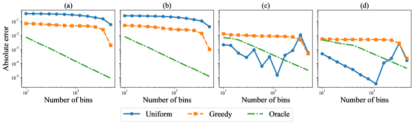
Figure 15: Absolute error versus number of bins for different quantization strategies with support size $600$ (log-log scale). (a): $\mathrm{Dir}(\mathbf{1})$ and $\mathrm{Dir}(\mathbf{1}/2)$; (b): $\mathrm{Zipf}(0)$ and $\mathrm{Dir}(\mathbf{1}/2)$; (c): $\mathrm{Zipf}(2)$ and Step; (d): $\mathrm{Zipf}(1)$ and $\mathrm{Zipf}(2)$.

G.2 Real data

We analyze the performance of the bounds as well as the various smoothed estimators in the context evaluating generative models for images and text using divergence curves. All experiments models are trained on a workstation with $8$ Nvidia Quadro RTX GPUs ($24$G memory each). The image experiments were trained with 2 GPUs at once while the text ones used all $8$.

Tasks and datasets. We consider two domains: images and text. For the image domain, we train a generative model for the CIFAR-10 dataset [36] based on StyleGAN2-Ada [32]. We use the publicly available code with their default hyperparameters and train on 2 GPUs. In order to enable the code to run faster, we make two architectural simplifications: (a) we reduce the channel dimensions for each convolution layer in the generator from $512$ to $256$, and, (b) we reduce the number of styled convolution layers for each resolution from $2$ to $1$. In particular, the latter effectively cuts the number of convolution layers in half. This leads to a 6.6x reduction in running time at the cost of a slightly worse FID [27] of $4.7$ rather than the $2.4$ of the original network. In order to compute the divergence frontier, we use the test set of $10000$ images as the target distribution $P$ and we sample $10000$ images from the generative model as the model distribution $Q$.

For the text domain, we finetune a pretrained GPT-2 [50] model with 124M parameters (i.e., GPT-2 small) on the Wikitext-103 dataset [43]. We use the open-source HuggingFace Transformers library [65] for training. To form a sufficiently large evaluation set, we finetune on 90% of the wikitext-103 training dataset, and use the remaining 10% plus the validation set as an evaluation set. Finetuning is done on 4 GPUs for 2k iterations, with sequences of 1024 tokens and a batch size of 8 sequences. For generation, we split the evaluation set into 10k sequences of 500 tokens, and split each sequence into a prefix of length 100 and a continuation of length 400. The prefix paired with the continuation (a “completion”) is considered a sample from $P$. Using the finetuned model we generate a continuation for each prefix using top-$p$ sampling with $p=0.9$. Each prefix paired with its generated continuation is considered a sample from $Q$.

Settings. In order to compute the divergence frontier, we jointly quantize $P$ and $Q$, not directly in a raw image/text space, but in a feature space [54, 37, 27]. Specifically, we represent each image by its features from a pretrained ResNet-50 model [25], and each text generation by its terminal hidden state under a pretrained the 774M GPT-2 model (i.e., GPT-2 large). In order to quantize these features, we learn a $4$ or $5$ dimensional embedding of the image/text features using a deep network which maintains the neighborhood structure of the data while encouraging the features to be uniformly distributed on the unit sphere [53], and simply quantize these embeddings on a uniform lattice with $k$ bins. For each support size $k$, this gives us quantized distributions $P_{\mathcal{S}_{k}},Q_{\mathcal{S}_{k}}$. We then sample $n$ i.i.d points each from these distributions and consider the empirical distributions $\hat{P}_{\mathcal{S}_{k},n},\hat{Q}_{\mathcal{S}_{k},n}$ as well as the add-constant and Good-Turing estimators computed form these samples. We repeat this $100$ times to a Monte Carlo estimate of the expected absolute error $\mathbb{E}|{\operatorname{FI}}(\hat{P}_{\mathcal{S}_{k},n},\hat{Q}_{\mathcal{S}_{k},n})-{\operatorname{FI}}(P_{\mathcal{S}_{k}},Q_{\mathcal{S}_{k}})|$ as well as its standard error.

Statistical error. We compare the distribution-dependent bound (“oracle bound”) and the distribution-free bound (“bound”) to the Monte Carlo estimates described above. We consider two experiments. First, we fix the support size $k$ and vary the sample size $n$ from $100$ to $25000$. Second, we fix the sample size $n$ and vary the support size $k$ from $8$ to $2048$ in powers of $2$.

We observe Fig. 16 that both the distribution-free and distribution-dependent bounds decrease with the sample size $n$ at a similar rate. For $k=1024$ or $k=2048$, we observe that the bound has approximately the same slope as the Monte Carlo estimate in log-log scale; this means that they exhibit a near-identical rate in $n$. On the other hand, the Monte Carlo estimates exhibit fast rates of convergence than the bound for $k=64$ or $k=128$. Therefore, the bounds capture the worst-case behavior of real image and text data.

Next, we see from Fig. 17 that the two bounds again exhibit near-identical rates with the support size $k$. We observe again that the slope of the Monte Carlo estimate and that of the bounds are close for $n=1000$, indicating a similar scaling with respect to $k$. However, the Monte Carlo estimate grows faster than the bound for $n=10000$.

Distribution estimators. As in the previous section, we compare the empirical estimator, the (modified) Good-Turing estimator, and three add-$b$ smoothing estimators, namely Laplace, Krichevsky-Trofimov and Braess-Sauer. We consider the same two experiments as for the statistical error.

From Fig. 18, we see that for $n>k$, we observe similar rates (i.e., similar slopes) for all estimators with respect to the sample size $n$. The absolute error of the Good-Turing estimator is the worst among all estimators considered for $k=64$ or $k=128$ and $n$ large. However, for $k=1024$ or $k=2048$, the empirical estimator is the worst. The various add-$b$ estimators work the best in the regime of $n<k$, where each add-$b$ estimator attains the smallest error at a different $n$. In particular, the Laplace estimator is the best or close to the best in all each of the settings considered.

Fig. 19 shows the corresponding results for varying $k$. The results are similar to the previous setting, expect the error increases with $k$ rather than decreases.

Performance across training. Next, we visualize the divergence frontiers and the corresponding frontier integral across training in Fig. 20. On the left, we plot the divergence curve at initialization (or with the pretrained model in case of text), at the first checkpoint (“Partly”) and the fully trained model (“Final”). We observe that the divergence frontiers for the fully trained model are closer to the origin than the partially trained ones or the model at initialization. This denotes a smaller loss of precision and recall for the fully trained model. The frontier integral, as a summary statistic, shows the same trend (right).

Table 3: The frontier integral with pretrained and finetuned feature embedding models.

Quantization level $k$ 2 4 8 16 32 64 128 256 512 1024 Pretrained 3.38e-5 2.64e-5 2.84e-4 6.95e-4 1.47e-3 3.25e-3 6.28e-3 1.18e-2 2.52e-2 5.09e-2 Finetuned 7.23e-6 1.37e-4 3.98e-4 1.77e-3 2.36e-3 5.31e-3 9.84e-3 1.95e-2 3.49e-2 6.34e-2

Fine-tuning the feature embedding model. In our real data experiments, we follow the common practice in this line of research [54, 18, 49] and use a pre-trained feature embedding model to extract feature representations. We also design a procedure to fine-tune the feature embedding model for comparing two distributions here. Concretely, we compare the frontier integral using the following two feature embedding models. First, we use a pretrained 4-layer ConvNet to extract feature embeddings for the generations of the StyleGAN. Second, we reinitialize the output layer of the 4-layer ConvNet, finetune it to distinguish true images from generated ones, and use the finetuned ConvNet to extract features. Finally, we compute the frontier integral using k-means clustering for various values of $k$. As shown in Tab. 3, the frontier integrals computed via the finetuned ConvNet are slightly larger than the ones without finetuning. This is as expected since the finetuned model usually gives a better feature representation in the sense of distinguishing distributions.

Figure 16: Absolute error versus sample size $n$ on real data (log-log scale) for the frontier integral (top) and the divergence frontier (bottom). Left Two: Image data (CIFAR-10) with support sizes $k=128$ and $k=1024$. Right Two: Text data (WikiText-103) with support sizes $k=64$ and $k=2048$. The bounds are scaled by $15$.

Figure 17: Absolute error versus support size $k$ on real data (log-log scale) for the frontier integral (top) and the divergence frontier (bottom). Left Two: Image data (CIFAR-10) with sample sizes $n=1000$ and $n=10000$ Right Two: Text data (WikiText-103) with sample sizes $n=1000$ and $n=10000$. The bounds are scaled by $15$.

Figure 18: Absolute error versus sample size $n$ on real data (log-log scale) for the frontier integral (top) and the divergence frontier (bottom). Left Two: Image data (CIFAR-10) with support size $k=128$ and $k=1024$ Right Two: Text data (WikiText-103) with support size $k=64$ and $k=2048$.

Figure 19: Absolute error versus support size $k$ on real data for the frontier integral (top) and the divergence frontier (bottom). Left Two: Image data (CIFAR-10) with sample sizes $n=1000$ and $n=10000$. Right Two: Text data (WikiText-103) with sample sizes $n=1000$ and $n=10000$.

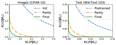
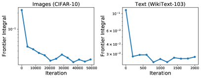
Figure 20: Left Two: The divergence frontier at different points in training. Right Two: The frontier integral plotted at different training checkpoints.

Appendix H Length of the divergence frontier

In this section, we discuss how the length of the divergence frontier is different from the frontier integral. In particular, we show that the length of the divergence frontier is lower bounded by the Jeffery divergence, which could be unbounded, whereas the frontier integral is always bounded between $0$ and $1$.

Setup. Let $P,Q$ be two distributions on a finite alphabet $\mathcal{X}$. Recall that the divergence frontier is defined as the parametric curve $\mathcal{F}(P,Q):=(x(\lambda),y(\lambda))$ for $\lambda\in(0,1)$ where

$$\begin{aligned} x(\lambda)&=\mathrm{KL}_{1-\lambda}(Q\|P)=\sum_{a\in\mathcal{X}}Q(a)\log\frac{Q(a)}{\lambda P(a)+(1-\lambda)Q(a)}\\ y(\lambda)&=\mathrm{KL}_{\lambda}(P\|Q)=\sum_{a\in\mathcal{X}}P(a)\log\frac{P(a)}{\lambda P(a)+(1-\lambda)Q(a)}\,.\end{aligned}$$ (25)

Recall that the Jeffery divergence between $P$ and $Q$ is defined as

$$\mathrm{JD}(P,Q)=\mathrm{KL}(P\|Q)+\mathrm{KL}(Q\|P)=\sum_{a\in\mathcal{X}}\big{(}P(a)-Q(a)\big{)}\big{(}\log P(a)-\log Q(a)\big{)}\,.$$

Note that $\mathrm{JD}(P,Q)$ is unbounded when there exists an atom such that $P(a)=0,Q(a)\neq 0$ or $P(a)\neq 0,Q(a)=0$.

We show that the length of the divergence frontier between $P,Q$ is lower bounded by the corresponding Jeffrey’s divergence, which can be unbounded.

Proposition 28.

Consider two distributions $P,Q$ on a finite alphabet $\mathcal{X}$. The length $\mathrm{length}(\mathcal{F}(P,Q))$ of the divergence frontier $\mathcal{F}(P,Q)$ satisfies

$$\mathrm{length}(\mathcal{F}(P,Q))\geq\frac{1}{\sqrt{2}}\mathrm{JD}(P,Q)\,.$$

Proof.

We assume without loss of generality that $P(a)+Q(a)>0$ for each $a\in\mathcal{X}$. Define shorthand $R_{\lambda}=\lambda P+(1-\lambda)Q$. We bound the length of the divergence frontier $\mathcal{F}(P,Q)$, which is given by $\int_{0}^{1}L(\lambda)\mathrm{d}\lambda$, as

$$L(\lambda)^{2} =x^{\prime}(\lambda)^{2}+y^{\prime}(\lambda)^{2}$$

$$=\left(\sum_{a\in\mathcal{X}}Q(a)\frac{Q(a)-P(a)}{R_{\lambda}(a)}\right)^{2}+\left(\sum_{a\in\mathcal{X}}P(a)\frac{Q(a)-P(a)}{R_{\lambda}(a)}\right)^{2}$$

$$\geq\frac{1}{2}\left(\sum_{a\in\mathcal{X}}\frac{(P(a)-Q(a))^{2}}{R_{\lambda}(a)}\right)^{2}=:\frac{1}{2}\widetilde{L}(\lambda)^{2}\,,$$

where we used the inequality $(a-b)^{2}\leq 2(a^{2}+b^{2})$ for $a,b\in\mathbb{R}$. We can now complete the proof by computing this integral as

$$\sqrt{2}\cdot\mathrm{length}(\mathcal{F}(P,q)) \geq\int_{0}^{1}\widetilde{L}(\lambda)\mathrm{d}\lambda$$

$$=\int_{0}^{1}\sum_{a\in\mathcal{X}}\frac{(P(a)-Q(a))^{2}}{R_{\lambda}(a)}\mathrm{d}\lambda$$

$$=\sum_{a\in\mathcal{X}}(P(a)-Q(a))^{2}\int_{0}^{1}\frac{1}{\lambda P(a)+(1-\lambda)Q(a)}\mathrm{d}\lambda$$

$$=\sum_{a\in\mathcal{X}}(P(a)-Q(a))(\log P(a)-\log Q(a))=\mathrm{JD}(P,Q)\,.$$

∎

Appendix I Technical lemmas

We state here some technical results used in the paper.

Theorem 29 (McDiarmid’s Inequality).

Let $X_{1},\cdots,X_{m}$ be independent random variables such that $X_{i}$ has range $\mathcal{X}_{i}$. Let $\Phi:\mathcal{X}_{1}\times\cdots\times\mathcal{X}_{n}\to\mathbb{R}$ be any function which satisfies the bounded difference property. That is, there exist constants $B_{1},\cdots,B_{n}>0$ such that for every $i=1,\cdots,n$ and $(x_{1},\cdots,x_{n}),(x_{1}^{\prime},\cdots,x_{n}^{\prime})\in\mathcal{X}_{1}\times\cdots\mathcal{X}_{n}$ which differ only on the $i$^th coordinate (i.e., $x_{j}=x_{j}^{\prime}$ for $j\neq i$), we have,

$$|\Phi(x_{1},\cdots,x_{n})-\Phi(x_{1}^{\prime},\cdots,x_{n}^{\prime})|\leq B_{i}\,.$$

Then, for any $t>0$, we have,

$${\mathbb{P}}\left(\left|\Phi(X_{1},\cdots,X_{n})-\mathbb{E}[\Phi(X_{1},\cdots,X_{n})]\right|>t\right)\leq 2\exp\left(-\frac{2t^{2}}{\sum_{i=1}^{n}B_{i}^{2}}\right)\,.$$

Property 30.

Suppose $f:(0,\infty)\to[0,\infty)$ is convex and continuously differentiable with $f(1)=0=f^{\prime}(1)$. Then, $f^{\prime}(x)\leq 0$ for all $x\in(0,1)$ and $f^{\prime}(x)\geq 0$ for all $x\in(1,\infty)$.

Proof.

Monotonicity of $f^{\prime}$ means that we have for any $x\in(0,1)$ and $y\in(1,\infty)$ that $f^{\prime}(x)\leq f^{\prime}(1)=0\leq f^{\prime}(y)$. ∎

Lemma 31.

For all $x\in(0,1)$ and $n\geq 3$, we have

$$0\leq(1-x)^{n}x\log\frac{1}{x}\leq\frac{\log n}{n}\,.$$

Proof.

Let $h(x)=(1-x)^{n}x\log(1/x)$ be defined on $(0,1)$. Since $\lim_{x\to 0}h(x)=0<h(1/n)$, the global supremum does not occur as $x\to 0$. We first argue that $h$ obtains its global maximum in $(0,1/n]$. We calculate

$$h^{\prime}(x)=(1-x)^{n-1}\left(-nx\log\frac{1}{x}+(1-x)\left(\log\frac{1}{x}-1\right)\right)\leq(1-x)^{n-1}(1-nx)\log\frac{1}{x}\,.$$

Note that $h^{\prime}(x)<0$ for $x>1/n$, so $h$ is strictly decreasing on $(1/n,1)$. Therefore, it must obtain its global maximum on $(0,1/n]$. On this interval, we have,

$$(1-x)^{n}x\log\frac{1}{x}\leq x\log\frac{1}{x}\leq\frac{\log n}{n}\,,$$

since $x\log(1/x)$ is increasing on $(0,\exp(-1))$. ∎

The next lemma comes from [3, Theorem 1].

Lemma 32.

For all $x\in(0,1)$ and $n\geq 1$, we have

$$0\leq(1-x)^{n}x\leq\exp(-1)/(n+1)<1/n\,.$$

References

• Alamgir et al. [2014] M. Alamgir, G. Lugosi, and U. von Luxburg. Density-preserving quantization with application to graph downsampling. In COLT, 2014.
• Benny et al. [2021] Y. Benny, T. Galanti, S. Benaim, and L. Wolf. Evaluation metrics for conditional image generation. International Journal of Computer Vision, 129(5), 2021.
• Berend and Kontorovich [2012] D. Berend and A. Kontorovich. The missing mass problem. Statistics & Probability Letters, 82(6), 2012.
• Binkowski et al. [2018] M. Binkowski, D. J. Sutherland, M. Arbel, and A. Gretton. Demystifying MMD GANs. In ICLR, 2018.
• Braess and Sauer [2004] D. Braess and T. Sauer. Bernstein polynomials and learning theory. Journal of Approximation Theory, 128(2), 2004.
• Brown et al. [2020] T. B. Brown, B. Mann, N. Ryder, M. Subbiah, J. Kaplan, P. Dhariwal, A. Neelakantan, P. Shyam, G. Sastry, A. Askell, S. Agarwal, A. Herbert-Voss, G. Krueger, T. Henighan, R. Child, A. Ramesh, D. M. Ziegler, J. Wu, C. Winter, C. Hesse, M. Chen, E. Sigler, M. Litwin, S. Gray, B. Chess, J. Clark, C. Berner, S. McCandlish, A. Radford, I. Sutskever, and D. Amodei. Language models are few-shot learners. In NeurIPS, 2020.
• Bu et al. [2018] Y. Bu, S. Zou, Y. Liang, and V. V. Veeravalli. Estimation of KL divergence: Optimal minimax rate. IEEE Transactions on Information Theory, 64(4), 2018.
• Cai et al. [2006] H. Cai, S. R. Kulkarni, and S. Verdú. Universal divergence estimation for finite-alphabet sources. IEEE Transactions on Information Theory, 52(8), 2006.
• Cai et al. [2011] T. T. Cai, X. J. Jeng, and J. Jin. Optimal detection of heterogeneous and heteroscedastic mixtures. Journal of the Royal Statistical Society: Series B (Statistical Methodology), 73(5), 2011.
• Chen et al. [2018] L. Chen, C. Tao, R. Zhang, R. Henao, and L. Carin. Variational inference and model selection with generalized evidence bounds. In ICML, 2018.
• Chen and Goodman [1999] S. F. Chen and J. Goodman. An empirical study of smoothing techniques for language modeling. Computer Speech & Language, 13(4), 1999.
• Church and Gale [1991] K. W. Church and W. A. Gale. A comparison of the enhanced Good-Turing and deleted estimation methods for estimating probabilities of English bigrams. Computer Speech & Language, 5, 1991.
• Clémençon and Vayatis [2009] S. Clémençon and N. Vayatis. Nonparametric estimation of the precision-recall curve. In ICML, pages 185–192, 2009.
• Clémençon and Vayatis [2010] S. Clémençon and N. Vayatis. Overlaying classifiers: a practical approach to optimal scoring. Constructive Approximation, 32:619–648, 2010.
• Cortes and Mohri [2005] C. Cortes and M. Mohri. Confidence intervals for the area under the ROC curve. In NeurIPS, volume 17, 2005.
• Dhariwal et al. [2020] P. Dhariwal, H. Jun, C. Payne, J. W. Kim, A. Radford, and I. Sutskever. Jukebox: A generative model for music. arXiv Preprint, 2020.
• Dieng et al. [2017] A. B. Dieng, D. Tran, R. Ranganath, J. W. Paisley, and D. M. Blei. Variational inference via $\chi$ upper bound minimization. In NeurIPS, 2017.
• Djolonga et al. [2020] J. Djolonga, M. Lucic, M. Cuturi, O. Bachem, O. Bousquet, and S. Gelly. Precision-recall curves using information divergence frontiers. In AISTATS, 2020.
• Flach [2012] P. Flach. Machine Learning: The Art and Science of Algorithms That Make Sense of Data. Cambridge University Press, 2012.
• Goldenshluger and Lepski [2009] A. Goldenshluger and O. Lepski. Structural adaptation via $\mathbb{L}_{p}$-norm oracle inequalities. Probability Theory and Related Fields, 143, 2009.
• Good [1953] I. J. Good. The population frequencies of species and the estimation of population parameters. Biometrika, 40(3-4), 1953.
• Györfi and Nemetz [1978] L. Györfi and T. Nemetz. $f$-dissimilarity: A generalization of the affinity of several distributions. Annals of the Institute of Statistical Mathematics, 30, 1978.
• Hämäläinen et al. [2020] P. Hämäläinen, T. Saloheimo, and A. Solin. Deep residual mixture models. arXiv Preprint, 2020.
• Han et al. [2020] Y. Han, J. Jiao, and T. Weissman. Minimax estimation of divergences between discrete distributions. IEEE Journal on Selected Areas in Information Theory, 1(3), 2020.
• He et al. [2016] K. He, X. Zhang, S. Ren, and J. Sun. Deep residual learning for image recognition. In CVPR, 2016.
• Hegde et al. [2004] A. Hegde, D. Erdogmus, T. Lehn-Schioler, Y. N. Rao, and J. C. Principe. Vector-quantization by density matching in the minimum Kullback-Leibler divergence sense. In IJCNN, 2004.
• Heusel et al. [2017] M. Heusel, H. Ramsauer, T. Unterthiner, B. Nessler, and S. Hochreiter. GANs trained by a two time-scale update rule converge to a local Nash equilibrium. In NeurIPS, 2017.
• Hulle [1999] M. V. Hulle. Faithful representations with topographic maps. Neural Networks, 12(6), 1999.
• Im et al. [2018] D. J. Im, H. Ma, G. W. Taylor, and K. Branson. Quantitatively evaluating GANs with divergences proposed for training. In ICLR, 2018.
• Ingster and Suslina [2003] Y. Ingster and I. Suslina. Nonparametric Goodness-of-Fit Testing Under Gaussian Models. Springer, 2003.
• Karras et al. [2019] T. Karras, S. Laine, and T. Aila. A style-based generator architecture for generative adversarial networks. In CVPR, 2019.
• Karras et al. [2020] T. Karras, M. Aittala, J. Hellsten, S. Laine, J. Lehtinen, and T. Aila. Training generative adversarial networks with limited data. In NeurIPS, 2020.
• Katz [1987] S. M. Katz. Estimation of probabilities from sparse data for the language model component of a speech recognizer. IEEE Transactions on Acoustics Speech and Signal Processing, 35(3), 1987.
• Kingma and Dhariwal [2018] D. P. Kingma and P. Dhariwal. Glow: Generative flow with invertible 1x1 convolutions. In NeurIPS, 2018.
• Krichevsky and Trofimov [1981] R. E. Krichevsky and V. K. Trofimov. The performance of universal encoding. IEEE Transactions on Information Theory, 27(2), 1981.
• Krizhevsky and Hinton [2009] A. Krizhevsky and G. Hinton. Learning multiple layers of features from tiny images. Technical Report, 2009.
• Kynkäänniemi et al. [2019] T. Kynkäänniemi, T. Karras, S. Laine, J. Lehtinen, and T. Aila. Improved precision and recall metric for assessing generative models. In NeurIPS, 2019.
• Lopez-Paz and Oquab [2017] D. Lopez-Paz and M. Oquab. Revisiting classifier two-sample tests. In ICLR, 2017.
• Mao et al. [2017] X. Mao, Q. Li, H. Xie, R. Y. K. Lau, Z. Wang, and S. P. Smolley. Least squares generative adversarial networks. In ICCV, 2017.
• Mcallester and Ortiz [2003] D. Mcallester and L. Ortiz. Concentration inequalities for the missing mass and for histogram rule error. Journal of Machine Learning Research, 4, 2003.
• McAllester and Schapire [2000] D. A. McAllester and R. E. Schapire. On the convergence rate of Good-Turing estimators. In COLT, 2000.
• Meinicke and Ritter [2002] P. Meinicke and H. Ritter. Quantizing density estimators. In NeurIPS, 2002.
• Merity et al. [2017] S. Merity, C. Xiong, J. Bradbury, and R. Socher. Pointer sentinel mixture models. In ICLR, 2017.
• Naeem et al. [2020] M. F. Naeem, S. J. Oh, Y. Uh, Y. Choi, and J. Yoo. Reliable fidelity and diversity metrics for generative models. In ICML, 2020.
• Nguyen et al. [2010] X. Nguyen, M. J. Wainwright, and M. I. Jordan. Estimating divergence functionals and the likelihood ratio by convex risk minimization. IEEE Transactions on Information Theory, 56(11), 2010.
• Nielsen and Bhatia [2013] F. Nielsen and R. Bhatia. Matrix Information Geometry. Springer, 2013.
• Orlitsky and Suresh [2015] A. Orlitsky and A. T. Suresh. Competitive distribution estimation: Why is Good-Turing good. In NeurIPS, 2015.
• Orlitsky et al. [2003] A. Orlitsky, N. P. Santhanam, and J. Zhang. Always Good Turing: Asymptotically optimal probability estimation. In FOCS, 2003.
• Pillutla et al. [2021] K. Pillutla, S. Swayamdipta, R. Zellers, J. Thickstun, S. Welleck, Y. Choi, and Z. Harchaoui. Mauve: Measuring the gap between neural text and human text using divergence frontiers. In NeurIPS, 2021.
• Radford et al. [2019] A. Radford, J. Wu, R. Child, D. Luan, D. Amodei, and I. Sutskever. Language models are unsupervised multitask learners. OpenAI Blog, 2019.
• Razavi et al. [2019] A. Razavi, A. van den Oord, and O. Vinyals. Generating diverse high-fidelity images with VQ-VAE-2. In NeurIPS, 2019.
• Rubenstein et al. [2019] P. K. Rubenstein, O. Bousquet, J. Djolonga, C. Riquelme, and I. O. Tolstikhin. Practical and consistent estimation of f-divergences. In NeurIPS, 2019.
• Sablayrolles et al. [2019] A. Sablayrolles, M. Douze, C. Schmid, and H. Jégou. Spreading vectors for similarity search. In ICLR, 2019.
• Sajjadi et al. [2018] M. S. M. Sajjadi, O. Bachem, M. Lucic, O. Bousquet, and S. Gelly. Assessing generative models via precision and recall. In NeurIPS, 2018.
• Salimans et al. [2016] T. Salimans, I. J. Goodfellow, W. Zaremba, V. Cheung, A. Radford, and X. Chen. Improved techniques for training GANs. In NeurIPS, 2016.
• Shorack [2000] G. R. Shorack. Probability for Statisticians. Springer, 2000.
• Silva and Narayanan [2007] J. Silva and S. Narayanan. Universal consistency of data-driven partitions for divergence estimation. In ISIT, 2007.
• Silva and Narayanan [2010] J. Silva and S. S. Narayanan. Information divergence estimation based on data-dependent partitions. Journal of Statistical Planning and Inference, 140(11), 2010.
• Simon et al. [2019] L. Simon, R. Webster, and J. Rabin. Revisiting precision recall definition for generative modeling. ICML, 2019.
• Sreekumar et al. [2021] S. Sreekumar, Z. Zhang, and Z. Goldfeld. Non-asymptotic performance guarantees for neural estimation of f-divergences. In AISTATS, 2021.
• Tao et al. [2018] C. Tao, L. Chen, R. Henao, J. Feng, and L. Carin. Chi-square generative adversarial network. In ICML, 2018.
• Verdú [2019] S. Verdú. Empirical estimation of information measures: A literature guide. Entropy, 21(8), 2019.
• Wang et al. [2005] Q. Wang, S. R. Kulkarni, and S. Verdú. Divergence estimation of continuous distributions based on data-dependent partitions. IEEE Transactions on Information Theory, 51(9), 2005.
• Wang et al. [2017] Y. Wang, D. Ramanan, and M. Hebert. Learning to model the tail. In NeurIPS, 2017.
• Wolf et al. [2020] T. Wolf, L. Debut, V. Sanh, J. Chaumond, C. Delangue, A. Moi, P. Cistac, T. Rault, R. Louf, M. Funtowicz, J. Davison, S. Shleifer, P. von Platen, C. Ma, Y. Jernite, J. Plu, C. Xu, T. L. Scao, S. Gugger, M. Drame, Q. Lhoest, and A. M. Rush. Transformers: State-of-the-art natural language processing. In EMNLP, 2020.
• Zellers et al. [2019] R. Zellers, A. Holtzman, H. Rashkin, Y. Bisk, A. Farhadi, F. Roesner, and Y. Choi. Defending against neural fake news. In NeurIPS, 2019.
• Zhang and Grabchak [2014] Z. Zhang and M. Grabchak. Nonparametric estimation of Küllback-Leibler divergence. Neural Computation, 26(11), 2014.