Abstract

We showcase the advantages of orbital-free density-potential functional theory (DPFT), a more flexible variant of Hohenberg–Kohn density functional theory. DPFT resolves the usual trouble with the gradient-expanded kinetic energy functional by facilitating systematic semiclassical approximations in terms of an effective potential energy that incorporates all interactions. With the aid of two systematic approximation schemes we demonstrate that DPFT is not only scalable, universally applicable in both position and momentum space, and allows kinetic and interaction energy to be approximated consistently, but can also compete with highly accurate, yet restricted, methods. As two- and three-dimensional geometries are extensively covered elsewhere, our focus here is on one-dimensional settings, with semiclassical observables systematically derived from both the Wigner function formalism and a split-operator approach. The high quality of our results for Fermi gases in Morse potentials invites the use of DPFT for describing more exotic systems, such as trapped large-spin fermion mixtures with contact or dipole-dipole interactions.

Chapter 0 DENSITY-POTENTIAL FUNCTIONAL THEORY
FOR FERMIONS IN ONE DIMENSION

1 Introduction

A gradient-free semiclassical particle density with enormous improvement over the Thomas–Fermi (TF) approximation [1, 2] has recently been developed for one-dimensional (1D) fermionic systems and applied to particle numbers as small as two [3, 4, 5] — a regime that is usually regarded as out of reach for the TF model. Ribeiro et al. in Ref. [3] deliver a systematic correction to TF (which we subsequently refer to as ‘RB15’): Despite the many approximations employed in arriving at the final expressions for particle density and kinetic energy, the derivations are void of ad hoc manipulations. Naturally, a systematic and scalable methodology beyond the TF approximation for systems in 1D, 2D, and 3D, which is both accurate and computationally efficient, would enjoy wide-spread application. However, RB15 is ultimately based on matching Langer-corrected WKB wave functions [6], such that the extension to 2D and 3D does not seem to be possible [7]. That should not distract, however, from the profound insight that “semiclassics is the hidden theory behind the success of DFT” [8].

Density-potential functional theory (DPFT) presents a unified framework for handling corrections to the TF approximation. The ground work for orbital-free DPFT was laid in the 1980s [9, 10, 11, 12, 13, 14, 15, 16] with the introduction of an effective potential alongside the particle density. The standard density-only energy-functional of Hohenberg–Kohn density functional theory [17, 18] is thereby transformed into a still exact, yet more flexible variant. Most importantly, the usual nightmare with gradient expansions of the kinetic energy in orbital-free DFT is avoided altogether (see the kinetic energy densities in Table 1, as functions of the one-particle density $n(\vecfont{r})$ at position $\vecfont{r}$). Moreover, approximations of kinetic energy and interaction energy can be made consistent. The latter trait is, for example, absent in Kohn–Sham (KS) DFT, where the interaction energy is subjected to your favorite approximation while the kinetic energy is exact.

The familiar leading gradient correction for dimension ${D=3}$, and its troublesome counterparts for ${D=1,2}$. We display the ground-state kinetic-energy densities $\tau^{\mathrm{TF}}[n]$ in Thomas–Fermi approximation and the leading corrections ${\tau^{\mathrm{sc}}[n]-\tau^{\mathrm{TF}}[n]}$ to order $\boldsymbol{\nabla}^{2}$ as presented in the literature. $m$ is the particle mass, $g$ is the spin multiplicity.  $D$ $\tau^{\mathrm{TF}}[n]$ $\tau^{\mathrm{sc}}[n]-\tau^{\mathrm{TF}}[n]$ References 1 $\displaystyle{\frac{\pi^{2}\hbar^{2}}{6m\,g^{2}}\bigl{(}n(x)\bigr{)}^{3}}$ $\displaystyle{-\frac{\hbar^{2}}{24m}\frac{\left(\partial_{x}n(x)^{\phantom{X}}\right)^{2}}{n(x)}}$ [19, 20, 21] 2 $\displaystyle{\frac{\pi\hbar^{2}}{m\,g}\bigl{(}n(\vecfont{r})\bigr{)}^{2}}$ $\displaystyle{\frac{\hbar^{2}}{24m}\,\delta\bigl{(}n(\vecfont{r})\bigr{)}\bigl{(}\boldsymbol{\nabla}n(\vecfont{r})\bigr{)}^{2}}$ [22, 23] 0 [19, 20, 21, 24] 3 $\displaystyle{\frac{\hbar^{2}}{5m}\left(\frac{3^{5}\pi^{4}}{2g^{2}}\right)^{1/3}\bigl{(}n(\vecfont{r})\bigr{)}^{5/3}}$ $\displaystyle{\frac{\hbar^{2}}{72m}\frac{\left(\boldsymbol{\nabla}n(\vecfont{r})^{\phantom{X}}\right)^{2}}{n(\vecfont{r})}}$ [19, 20, 21, 25]

The purpose of the present article is two-fold: First, we introduce DPFT and extend our previous works on two- and three-dimensional geometries [26, 27, 28, 29] to the 1D setting. Specifically, we illustrate the workings of DPFT within two disjunct approaches: (i) we deploy systematic gradient expansions in the effective potential using Wigner’s phase space formalism, see [26, 27] and references therein; (ii) we utilize a split-operator approach to retrieve a hierarchy of approximations without a gradient expansion, see [28] and references therein. Second, we derive and benchmark densities and energies against the exact values for up to 1000 noninteracting fermions in a 1D Morse potential. These examples demonstrate that DPFT can deliver accuracies of energies and particle densities that are of similar quality as those obtained from RB15 [3, 4, 5]. While RB15 works for one-dimensional problems only, there is nothing special about 1D from the DPFT perspective, where particle densities and energies can be derived within various frameworks in a unified way for all geometries.

2 Density-potential functional theory in a nutshell

We start from Hohenberg–Kohn DFT, which aims at finding the extremum of the density functional of the total energy

$$E=E[n,\mu]=E_{\mathrm{kin}}[n]+E_{\mathrm{ext}}[n]+E_{\mathrm{int}}[n]+\mu\left(N-\int(\mathrm{d}\vecfont{r})\,n(\vecfont{r})\right)$$ (1)

(composed of kinetic, external, and interaction energy) of a system constrained to $N$ particles via the chemical potential $\mu$. We introduce the effective potential energy by

$$V(\vecfont{r})=\mu-\frac{\delta E_{\mathrm{kin}}[n]}{\delta n(\vecfont{r})}$$ (2)

and write

$$E_{1}[V-\mu]=E_{\mathrm{kin}}[n]+\int(\mathrm{d}\vecfont{r})\,\bigl{(}V(\vecfont{r})-\mu\bigr{)}\,n(\vecfont{r})$$ (3)

for the Legendre transform of the kinetic energy functional $E_{\mathrm{kin}}[n]$, such that

$$E= \;E[V,n,\mu]$$

$$= \;E_{1}[V-\mu]-\int(\mathrm{d}\vecfont{r})\,n(\vecfont{r})\,\bigl{(}V(\vecfont{r})-V_{\mathrm{ext}}(\vecfont{r})\bigr{)}+E_{\mathrm{int}}[n]+\mu N\,.$$ (4)

At the stationary point of $E[V,n,\mu]$, the $V$- and $n$-variations obey

$$\delta V: \qquad\,n[V,\mu](\vecfont{r})=\frac{\delta E_{1}[V-\mu]}{\delta V(\vecfont{r})}$$ (5)

and

$$\delta n: \qquad V[n](\vecfont{r})=V_{\mathrm{ext}}(\vecfont{r})+\frac{\delta E_{\mathrm{int}}[n]}{\delta n(\vecfont{r})}\,,$$ (6)

respectively. The $\mu$-variation, combined with Eq. (5), reproduces the particle-number constraint

$$\int(\mathrm{d}\vecfont{r})\,n(\vecfont{r})=N\,.$$ (7)

Equation (5) immediately yields the particle density in the noninteracting case (${V=V_{\mathrm{ext}}}$). For a given value of $\mu$, $n$ is a functional of $V$, and vice versa, such that a self-consistent solution of Eqs. (5)—(7) in the case of interacting systems produces the ground-state density, much like in the KS scheme, but without resorting to orbitals. Details of the numerical implementation of the self-consistent loop for DPFT can be found in Appendix E of Ref. [29]. Further details and implications of Eqs. (2)–(7) are well documented in the literature, see [15, 26, 27, 30], for example.

While $E_{\mathrm{kin}}[n]$ is not known explicitly, it is a simple exercise to find the single-particle trace

$$E_{1}[V-\mu]=\mathrm{tr}\bigl{(}\mathcal{E}_{T}(H-\mu)\bigr{)}\,,$$ (8)

for independent particles, see Refs. [27, 30], with the ground-state version recovered as the temperature $T$ tends to zero. Here, the operator

$$\mathcal{E}_{T}(A=H-\mu)=(-k_{\mathrm{B}}T)\,\ln\Bigl{(}1+\mathrm{e}^{-A/(k_{\mathrm{B}}T)}\Bigr{)}$$ (9)

is a function of the single-particle Hamiltonian

$$H(\vecfont{R},\vecfont{P})=\frac{\vecfont{P}^{2}}{2m}+V(\vecfont{R})\,,$$ (10)

where $\vecfont{R}$ and $\vecfont{P}$ are the single-particle position and momentum operators, respectively. Equation (8) and its zero-temperature limit are exact for noninteracting systems and can be made exact for interacting systems if the interacting part of the kinetic-energy density-functional is transferred from Eq. (3) to $E_{\mathrm{int}}[n]$.

Any approximation of the single-particle trace in Eq. (8) yields a corresponding approximation for the particle density in Eq. (5). We are now in the position to benchmark semiclassical approximations of $E_{1}$ unambiguously for systems with a known interaction functional and for noninteracting systems.

We shall employ and explore two independent approximation schemes for DPFT. First, as worked out in Ref. [27], we express the trace in Eq. (8) as the classical phase space integral

$$\mathrm{tr}\Bigl{(}\mathcal{E}_{T}\bigl{(}A(\vecfont{R},\vecfont{P})\bigr{)}\Bigr{)}=g\int\frac{(\mathrm{d}\vecfont{r})(\mathrm{d}\vecfont{p})}{(2\pi\hbar)^{D}}\,\bigl{[}\mathcal{E}_{T}(A)\bigr{]}_{\mathrm{W}}(\vecfont{r},\vecfont{p})\,,$$ (11)

where the momentum integral over the Wigner function $\big{[}\mathcal{E}_{T}(A)\big{]}_{\mathrm{W}}$ of $\mathcal{E}_{T}(A)$ can be approximated by

$$\int(\mathrm{d}\vecfont{p})\,\big{[}\mathcal{E}_{T}(A)\big{]}_{\mathrm{W}}(\vecfont{r},\vecfont{p})\cong\int(\mathrm{d}\vecfont{p})\,{\left\langle\!\mathcal{E}_{T}\bigl{(}\tilde{A}_{\mathrm{W}}\bigr{)}-\frac{\hbar^{2}\left(\boldsymbol{\nabla}^{2}V\right)}{12m}\mathcal{E}_{T}^{\prime\prime}\bigl{(}\tilde{A}_{\mathrm{W}}\bigr{)}\!\right\rangle}_{\mathrm{Ai}}.\rule[-18.0pt]{0.0pt}{5.0pt}$$ (12)

Here,

$$\tilde{A}_{\mathrm{W}}(\vecfont{r},\vecfont{p})=H_{\mathrm{W}}(\vecfont{r},\vecfont{p})-\mu-x\,a(\vecfont{r})\,,$$ (13)

with the Wigner function ${H_{\mathrm{W}}(\vecfont{r},\vecfont{p})=\vecfont{p}^{2}/(2m)+V(\vecfont{r})}$ of the single-particle Hamiltionian and ${a(\vecfont{r})=|\hbar\boldsymbol{\nabla}V(\vecfont{r})|^{2/3}/(2m^{1/3})}$. Equation (12) is exact up to the leading gradient correction $\left[\mathcal{O}\left(\boldsymbol{\nabla}^{2}\right)\right]$, and thus presents a systematic correction to the TF approximation, which is recovered in the uniform limit $\left[\mathcal{O}\left(\boldsymbol{\nabla}^{0}\right)\right]$. However, the ‘Airy-average’ in Eq. (12) contains also higher-order gradient corrections that enter through the Moyal products from the power series expansion of $\mathcal{E}_{T}(A)$ in Eq. (11). These higher-order corrections are responsible for the almost exact behavior of particle densities across the boundary between classically allowed and forbidden regions, where the TF approximation can fail epically (even if supplemented with the leading gradient correction [27]). We obtain the approximate particle densities for one-, two-, and three-dimensional geometries by combining Eqs. (5) and (8)–(13) and evaluating the momentum integral of Eq. (12). The 2D case is covered extensively in Refs. [26, 27], and a manuscript that covers the 3D formulae, in particular for computational chemistry, is in preparation [31]. Here, we focus on the 1D situation and provide details in Secs. 3 and 5.

Our second approximation scheme reiterates some of the results in Ref. [28] and begins with realizing that Eqs. (5) and (8) at ${T=0}$ yield

$$n(\vecfont{r})=g\left\langle\right.{\vecfont{r}}\left.\right|{\eta(\mu-H)}\left|\right.{\vecfont{r}}\left.\right\rangle=g\int\limits_{\begin{picture}(16.0,3.0)(-8.0,-3.0)\put(0.0,0.0){\curve(-3,0,-8,0)\curve(3,0,8,0)}\put(8.0,0.0){\curve(0,0,-1.5,1.5)\curve(0,0,-1.5,-1.5)}\put(0.0,0.0){\arc(-3,0){180}}\put(0.0,0.0){\makebox(0.0,0.0)[]{$\cdot$}}\end{picture}}\frac{\mathrm{d}t}{2\pi\mathrm{i}t}\,\mathrm{e}^{\frac{\mathrm{i}t}{\hbar}\mu}\,\left\langle\right.{\vecfont{r}}\left.\right|{U(t)}\left|\right.{\vecfont{r}}\left.\right\rangle\,,$$ (14)

which invites tailored Suzuki–Trotter (ST) factorizations of the unitary time-evolution operator ${U(t)=\mathrm{e}^{-\frac{\mathrm{i}t}{\hbar}H}}$. We obtain a hierarchy of approximations of $n(\vecfont{r})$ from appropriate coefficients $\alpha_{i}$ and $\beta_{i}$ in the ansatz

$$U(t)\approx U_{\nu}(t)=\prod_{i=1}^{\lceil\nu/2\rceil}\mathrm{e}^{-\frac{\mathrm{i}t}{\hbar}\alpha_{i}V(\vecfont{R})}\,\mathrm{e}^{-\frac{\mathrm{i}t}{\hbar}\beta_{i}\vecfont{P}^{2}/(2m)}\,,$$ (15)

where the exponential factors are multiplied from left to right in order of increasing $i$ values. The choice ${\alpha_{1}=0}$, ${\alpha_{2}=1}$, and ${\beta_{1}=\beta_{2}=1/2}$ yields

$$n_{3^{\prime}}(\vecfont{r})=g\int(\mathrm{d}\vecfont{a})\left(\frac{k_{3^{\prime}}}{2\pi a}\right)^{D}\mathrm{J}_{D}\bigl{(}2ak_{3^{\prime}}\bigr{)}\,,$$ (16)

with $k_{3^{\prime}}=\frac{1}{\hbar}\big{[}2m\,\bigl{(}\mu-V(\vecfont{r}+\vecfont{a})\bigr{)}\big{]}_{+}^{1/2}$, ${[z]_{+}=z\,\eta(z)}$, and $\mathrm{J}_{D}(\ )$ the Bessel function of order $D$. Equation (16) is a first nonlocal correction to the TF density, since $U_{3^{\prime}}(t)$ recovers $U(t)$ up to $\mathcal{O}(t^{2})$. Reference [28] also features an approximation $n_{7}$ for the particle density based on merely five exponential factors,

$$\alpha_{1}=\alpha_{3}=\frac{1}{6}\,,\quad\alpha_{2}V=\frac{2}{3}V-\frac{1}{72m}[t\boldsymbol{\nabla}V]^{2}\,,$$

$$\beta_{1}=\beta_{3}=\frac{1}{2}\,,\quad\beta_{2}=0\,,$$ (17)

instead of the eleven factors needed for reaching the same order of accuracy $\left[\mathcal{O}\left(t^{4}\right)\right]$ if $\alpha_{i}$ and $\beta_{i}$ are required to be constants [37]: Equation (14) with Eqs. (15) and (2) yields

$$n(\vecfont{r})\cong n_{7}(\vecfont{r})={\left\langle g\int(\mathrm{d}\vecfont{a})\,{\left(\frac{k^{(x)}_{7}}{2\pi a}\right)}^{D}\mathrm{J}_{D}{\left(2ak^{(x)}_{7}\right)}\right\rangle}_{\mathrm{Ai}}\,,$$ (18)

where

$$k^{(x)}_{7} =\frac{1}{\hbar}\Biggl{[}2m{\left(\mu-\frac{1}{3}\bigl{[}V(\vecfont{r})+2V(\vecfont{r}+\vecfont{a})\bigr{]}\right)}$$

$$\hphantom{=\frac{1}{\hbar}\Biggl{[}}\mbox{}-x{\left(\frac{1}{3}\bigl{[}\hbar m\boldsymbol{\nabla}V(\vecfont{r}+\vecfont{a})\bigr{]}^{2}\right)}^{1/3}\Biggr{]}^{1/2}_{+}\,.$$ (19)

Since $n_{7}$ is exact up to fourth order in $t$, it is exact for the linear potential and includes the leading gradient correction. In contrast to the local TF density, $n_{3^{\prime}}(\vecfont{r})$ and $n_{7}(\vecfont{r})$ are fully nonlocal expressions, which sample the effective potential $V$ in a neighborhood of the position $\vecfont{r}$, and can provide highly accurate density profiles, as tested for 3D in Ref. [28]. We assess the quality of Eqs. (16) and (18) for ${D=1}$ in Sec. 4 below.

3 Airy-averaged densities in 1D

The semiclassical particle densities from the Wigner function approach in 1D and 3D can be obtained analogously to the 2D case covered in Ref. [27]. We now focus on the 1D situation, for which the so far available orbital-free gradient corrections of the kinetic energy are not bounded from below, see Table 1. The semiclassical closed expression RB15 for the particle density [3] proves to be remarkably accurate even for two particles, and also in the vicinity of the classical turning points, where the failure of the TF approximation is most pronounced. We will show in the following that, like in 2D, the Airy-averaged densities of our DPFT formalism closely resemble the exact densities everywhere for very low but finite temperatures. Even for ${N=2}$ our Airy-averaging method delivers a high accuracy.

As outlined in Sec. 2, Eq. (5) eventually yields

$$n(r,T)\cong n^{\mathrm{Ai}}(r,T)=g\frac{\sqrt{2m}}{\pi\hbar}\left\langle\right.{b_{x}(r)\,l_{x}(r,T)}\left.\right\rangle_{\mathrm{Ai}}$$ (20)

for ${V^{\prime}\not=0}$, where

$$b_{x}(r) =1-\frac{\hbar^{2}U^{\prime\prime}(r)}{12m\,a(r)^{2}}x\,,$$

$$l_{x}(r,T) =-\frac{\sqrt{\pi k_{\mathrm{B}}T}}{2}\mathrm{Li}_{1/2}\Bigl{(}-\mathrm{e}^{\left[x\,a(r)-U(r)\right]/(k_{\mathrm{B}}T)}\Bigr{)},$$

$$l_{x}(r,0) =\sqrt{a(r)}\,\sqrt{x-y(r)}\,\eta\bigl{(}x-y(r)\bigr{)}\,,$$

$$y(r) =U(r)/a(r)\,,$$

$$U(r) =V(r)-\mu\,,$$ (21)

${U^{\prime}(r)=\partial_{r}U(r)}$, ${U^{\prime\prime}(r)=\partial_{r}^{2}U(r)}$, and $\mathrm{Li}_{1/2}(\ )$ is the polylogarithm of order $1/2$. With ${\tilde{A}_{\mathrm{W}}\to A_{\mathrm{W}}}$ for ${V^{\prime}\to 0}$, the Airy-average in Eq. (12) drops out, and we find

$$n^{\mathrm{Ai}}\bigl{(}\left.r\right|_{V^{\prime}=0},T\bigr{)} =-\frac{g}{\hbar}\sqrt{\frac{m\,k_{\mathrm{B}}T}{2\pi}}\mathrm{Li}_{1/2}\Bigl{(}-\mathrm{e}^{-U/(k_{\mathrm{B}}T)}\Bigr{)}$$

$$\phantom{=}-\frac{g\,\hbar\,U^{\prime\prime}}{96\,\pi\,m\,(k_{\mathrm{B}}T)^{2}}\int\mathrm{d}p\,\frac{\sinh\bigl{(}\gamma(p)\bigr{)}}{\bigl{[}\cosh\bigl{(}\gamma(p)\bigr{)}\bigr{]}^{3}}\,,$$ (22)

where ${\gamma(p)=A_{\mathrm{W}}/(2k_{\mathrm{B}}T)}$.

The zero-temperature limit of the density expression in Eq. (20) reads

$$n^{\mathrm{Ai}}(r,0) =g\frac{p_{\mathrm{F}}}{\hbar}\Biggl{[}-\mathrm{sgn}(\bar{y})\,\sqrt{|\bar{y}|}\,\mathrm{Ai}(\bar{y})^{2}+\frac{\mathrm{Ai}^{\prime}(\bar{y})^{2}}{\sqrt{|\bar{y}|}}$$

$$\hphantom{=g\frac{p_{\mathrm{F}}}{\hbar}\Biggl{[}}+\frac{\hbar\,U^{\prime\prime}}{3\,p_{\mathrm{F}}\,|U^{\prime}|}\mathrm{Ai}(\bar{y})\mathrm{Ai}^{\prime}(\bar{y})\Biggr{]}\,,$$ (23)

with the local Fermi momentum ${p_{\mathrm{F}}=\sqrt{2m|U(r)|}}$ and ${\bar{y}=2^{-2/3}y(r)}$. The Airy-averaged ground-state density in Eq. (3) holds for ${U\not=0}$ (and ${U^{\prime}\not=0}$) and exhibits a striking structural resemblance to the expression of the semiclassical particle density RB15 given in Ref. [3], although the latter is void of gradients of the potential. While beyond the scope of this article, we deem it a worthy enterprise to explore the deeper connections between RB15 and Eq. (3). This may possibly lead to a cure for the unphysical oscillations of $n^{\mathrm{Ai}}(r,0)$ near the extremal points of $U$, see Fig. 1 below.

4 DPFT densities for the Morse potential

For our benchmarking exercise we refrain from considering the harmonic oscillator potential, for which the TF energy of noninteracting spin-polarized (${g=1}$) fermions in 1D accidentally coincides with the exact energy (for integer $N$). As in Ref. [3], we rather opt for the Morse potential

$$V_{\mathrm{ext}}(r)=V_{0}\,\left(e^{-r/2}-2e^{-r/4}\right)$$ (24)

of depth $V_{0}$.

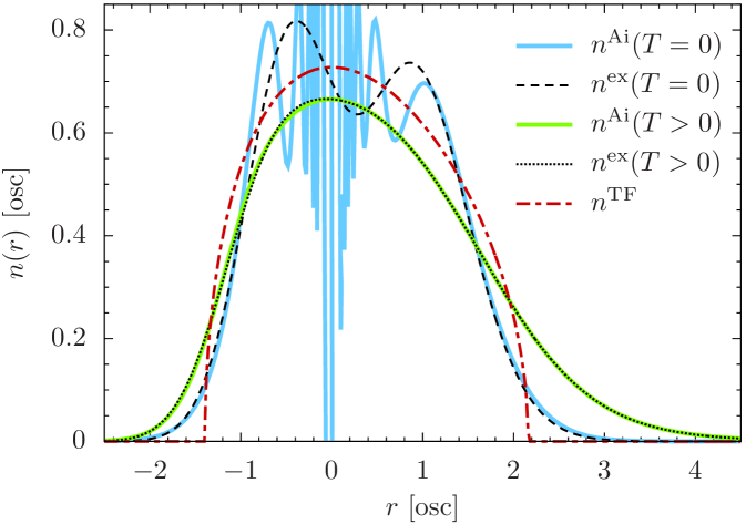
Figure 1: Particle densities for the 1D Morse potential in Eq. (24) with ${V_{0}=15}$. While $n^{\mathrm{Ai}}(r,T>0)$ (${k_{\mathrm{B}}T=1}$) agrees well with the exact density $n^{\mathrm{ex}}(r,T>0)$ everywhere, in particular near the classical turning points, $n^{\mathrm{Ai}}(r,0)$ exhibits unphysical oscillations that are due to the second line of Eq. (3), which diverges as ${U^{\prime}\to 0}$. For the 2D case, similar oscillations are linked to an ill-defined zero-temperature limit, see [27]. RB15 from Ref. [3] essentially coincides with ${n^{\mathrm{ex}}(r,T=0)}$.

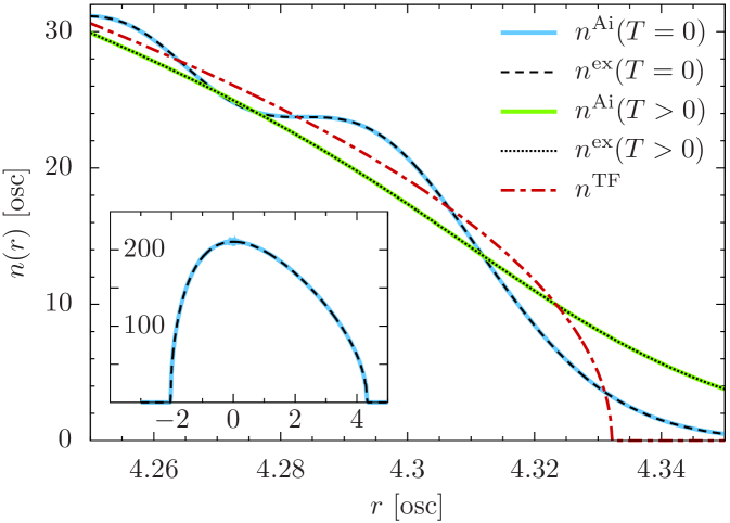
Figure 2: Particle densities as in Fig. 1, but for ${N=1000}$ fermions, with ${V_{0}=5\times 10^{5}}$ and ${k_{\mathrm{B}}T=1000}$. Evidently, both $n^{\mathrm{Ai}}(r,T)$ and $n^{\mathrm{Ai}}(r,0)$ leave nothing to be desired in the vicinity of the classical turning points (main plot). The inset shows that the unphysical oscillations of $n^{\mathrm{Ai}}(r,0)$ near the minimum of the Morse potential are much better behaved for ${N=1000}$ than for ${N=2}$, which stresses the fact that $n^{\mathrm{Ai}}$ is a semiclassical approximation.

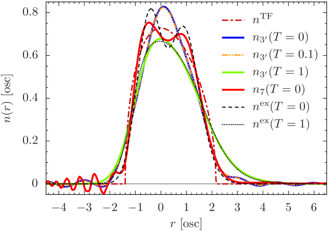
Figure 3: Compared with the Airy-averaged density $n^{\mathrm{Ai}}$ in Fig. 1, the density tails and the finite-temperature profiles of $n_{3^{\prime}}$ are less accurate, but they are well-behaved at any temperature. $n_{7}$ qualitatively captures the exact oscillations in the classically allowed region but exhibits unphysical oscillations in the classically forbidden region (at negative $r$), where large gradients of $V$ pose a challenge.

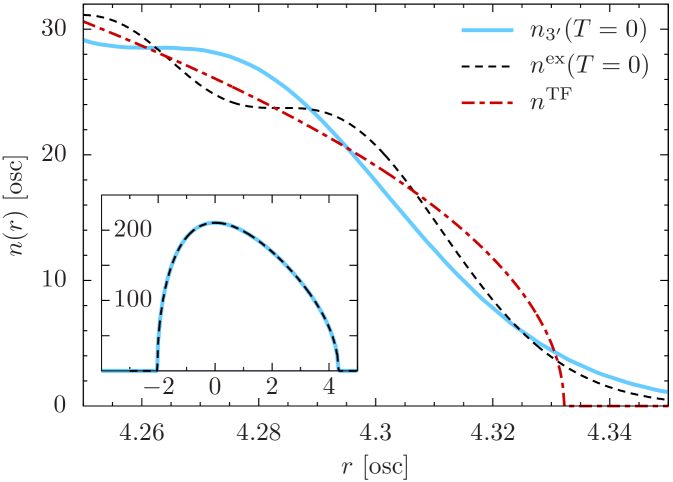
Figure 4: Like Fig. 2, but with the density formula $n_{3^{\prime}}$ of Eq. (16). As expected, $n_{3^{\prime}}$ captures the exact density profile reasonably well (inset), but does not match the oscillations into the classically forbidden region (main plot) — $n_{3^{\prime}}$ is not exact for a linear potential, in contrast to $n^{\mathrm{Ai}}$.

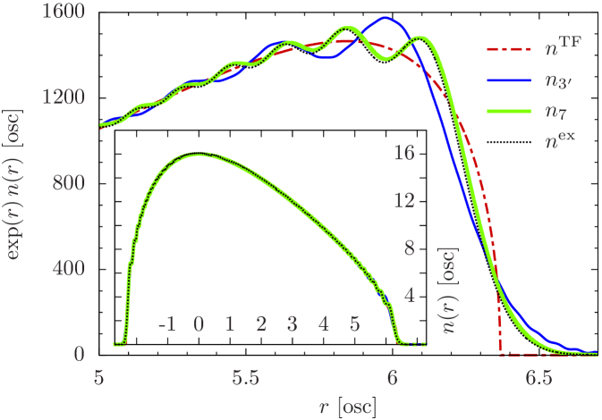
Figure 5: In the semiclassical regime of ${N=100}$ fermions and ${V_{0}=2000}$, $n_{7}$ captures the oscillatory behavior of the exact density with excellent accuracy. The deviations from $n^{\mathrm{ex}}$ in the tail are only visible when exponentially amplified (main plot). As expected, $n_{7}$ proves superior to $n_{3^{\prime}}$, whose oscillations are out of phase with the exact oscillations.

Figure 1 illustrates the high quality of our Airy-averaged densities for two fermions in the vicinity of the classical turning points, where they are designed to perform well. We compare the Airy-averaged expressions $n^{\mathrm{Ai}}(r,T)$ and $n^{\mathrm{Ai}}(r,0)$ with the exact densities $n^{\mathrm{ex}}$ [38] and the (zero-temperature) TF density $n^{\mathrm{TF}}$. Bearing in mind that the TF approximation is not well suited for small particle numbers, the corrections to TF included in $n^{\mathrm{Ai}}(r,T)$ deliver a remarkable accuracy. As expected, this observation is even more striking for larger particle numbers: We demonstrate in Fig. 2 that our Airy-averaged densities are indistinguishable (to the eye) from the exact densities near the classical turning points for ${N=1000}$ fermions.

In the following, we assess the semiclassical density expressions $n_{3^{\prime}}(\vecfont{r})$ and $n_{7}(\vecfont{r})$, based on the Suzuki–Trotter approximations in Eq. (15). Figure 3 shows the density of two noninteracting particles in the Morse potential with $n_{3^{\prime}}$ of Eq. (16) — the simplest variant of $n_{\nu}$ beyond the TF approximation — and $n_{7}$ from Eq. (18). The derivation of the finite-temperature version ${n_{3^{\prime}}(T>0)}$ is given elsewhere [39, 31]. Oscillations around zero in the classically forbidden region appear for both $n_{3^{\prime}}$ and $n_{7}$. That is, the higher-order errors of $n_{\nu}$ cannot be regarded small for some effective potentials $V$ — like the Morse potential whose gradient diverges exponentially. However, these errors diminish for larger particle numbers: Increasing the particle number to ${N=1000}$ in the deep Morse potential ${\left(V_{0}=5\times 10^{5}\right)}$, we approach the quasiclassical regime, where the TF density and its semiclassical corrections are largely indistinguishable (to the eye) from the exact density, see Fig. 4. In Fig. 5 we showcase the quasi-exact behavior of $n_{7}$ for a moderate particle number of ${N=100}$, for which the exact quantum oscillations are still visible to the eye and where the semiclassical DPFT densities deliver, unsurprisingly, a much higher accuracy compared with the case of ${N=2}$.

5 Airy-averaged energies

We conclude with the benchmarking of the semiclassical energies of our Wigner function approach. The zero-temperature Airy-average of the potential functional $E_{1}[U]$ for polarized Fermi gases in 1D is obtained from Eqs. (8)–(13) and reads

$$E_{1}^{\mathrm{Ai}}[U]=\int\mathrm{d}r\,{\left[\frac{U^{\prime\prime}}{6}{\left(\frac{\hbar^{2}}{2m|U^{\prime}|}\right)}^{1/3}F_{0}(\bar{y})-\bigl{|}U^{\prime}\bigr{|}F_{2}(\bar{y})\right]}\,,$$ (25)

where ${F_{2}(\bar{y})=\frac{2}{3}\bigl{[}\bar{y}^{2}\mathrm{Ai}(\bar{y})^{2}-\frac{1}{2}\mathrm{Ai}(\bar{y})\mathrm{Ai}^{\prime}(\bar{y})-\bar{y}\mathrm{Ai}^{\prime}(\bar{y})^{2}\bigr{]}}$ and ${F_{0}(\bar{y})=\mathrm{Ai}(\bar{y})^{2}}$, see Ref. [15]. While the oscillations of $n^{\mathrm{Ai}}(r,0)$ become singular as ${U^{\prime}\to 0}$, the integrand of $E_{1}^{\mathrm{Ai}}[U]$ remains finite throughout. An analogous observation holds for the 2D case [27].

We assess the performance of $E_{1}^{\mathrm{Ai}}[U]$ for the 1D Morse potential in Eq. (24). In Table 5 we report the total energies for several particle numbers $N$. The Airy-averaged energies show a significant improvement over the TF energies if the particle densities differ considerably from those of the harmonic oscillator, that is, if the chemical potential is close to the bound-state threshold.

The comparison of ${E^{\mathrm{Ai}}=E_{1}^{\mathrm{Ai}}+\mu^{\mathrm{Ai}}N}$, see Eqs. (2) and (25), with the exact energies $E^{\mathrm{ex}}$ (see Ref. [38]) for the 1D Morse potential in Eq. (24) reveals a satisfactory performance of the Airy-averaged energy functional in Eq. (25). The improvement of $E^{\mathrm{Ai}}$ over the TF energy $E^{\mathrm{TF}}$ is most visible if $N$ is close to the number $N_{\mathrm{max}}$ of bound states supported by $V_{0}$, i.e., if the part of $V$ that is most relevant for the density profile is least harmonic. $V_{0}$ 0.25 2.5 15 15 15 ${3.2\times 10^{4}}$ ${5\times 10^{5}}$ $N$[$N_{\mathrm{max}}$] 2[3] 8[9] 2[22] 8[22] 20[22] 1000[1012] 1000[4000] $E^{\mathrm{ex}}$ -0.2246 -27.340 -81.495 -7.424 -109.420 -10793887.5 -385416664 $E^{\mathrm{TF}}$ -0.2298 -27.345 -81.516 -7.445 -109.472 -10793890.1 -385416667 $E^{\mathrm{Ai}}$ -0.2231 -27.288 -81.459 -7.423 -109.416 -10793887.4 -385416656

The value $E_{\mathrm{kin}}^{\mathrm{Ai}}$ of the Airy-averaged kinetic energy at the stationary point of $E[V,n,\mu]$ can also be evaluated unambiguously. Employing Eq. (B.15) from Ref. [27],

$$\int(\mathrm{d}\vecfont{p})\,\frac{\vecfont{p}^{2}}{2m}\,\big{[}f(A)\big{]}_{\mathrm{W}}(\vecfont{r},\vecfont{p})$$

$$\cong \int(\mathrm{d}\vecfont{p})\,\frac{\vecfont{p}^{2}}{2m}{\left\langle f\bigl{(}\tilde{A}_{\mathrm{W}}\bigr{)}-\frac{\hbar^{2}\left(\boldsymbol{\nabla}^{2}V\right)}{12m}\frac{D-1}{D}f^{\prime\prime}\bigl{(}\tilde{A}_{\mathrm{W}}\bigr{)}\right\rangle}_{\mathrm{Ai}}\,,$$ (26)

which holds for any function $f$ that has a Fourier transform, we find

$$E_{\mathrm{kin}}^{\mathrm{Ai}} =\mathrm{tr}{\left\{\frac{P^{2}}{2m}\eta(\mu-H)\right\}}$$

$$=\frac{g}{2\pi\hbar}\int\mathrm{d}r\,\mathrm{d}p\,\frac{p^{2}}{2m}{\left\langle\eta\bigl{(}x\,a-U-p^{2}/(2m)\bigr{)}\right\rangle}_{\mathrm{Ai}}$$

$$=g\int\mathrm{d}r\,\frac{|U^{\prime}|}{2}\,F_{2}(\bar{y})$$ (27)

for ${D=1}$ after performing the momentum integral and the Airy average in Eq. (27). At the ground state itself, the energies in Table 5 are indeed reproduced by ${E_{\mathrm{kin}}^{\mathrm{Ai}}+\int\mathrm{d}r\,V_{\mathrm{ext}}(r)\,n^{\mathrm{Ai}}(r,0)}$, with ${V=V_{\mathrm{ext}}}$ in the noninteracting case. In contrast to $E_{1}^{\mathrm{Ai}}[U]$, however, Eq. (27) holds at the ground state only and can therefore not be used as a functional for determining the stationary points of the total energy.

6 Concluding remarks

This presentation puts a spotlight on foundations and recent advances of density-potential functional theory. We complemented our technical arsenal for two- and three-dimensional settings, see Refs. [27, 28, 29] and references therein, by deriving systematic corrections to the Thomas–Fermi approximation for both densities and energies in one dimension. Benchmarking against exact values for noninteracting fermions in a Morse potential at both zero and finite temperature, we found that our ‘Airy-averaged’ Wigner function approach delivers highly accurate density tails across the boundary of the classically allowed region and can improve significantly upon the already very accurate Thomas–Fermi energies. We also demonstrated that our most accurate split-operator-based density formula ($n_{7}$) delivers the quantum oscillations of the exact densities. Our results underscore the high quality of our semiclassical techniques when used in conjunction with an accurate interaction functional. In other words, the kinetic energy is handled accurately without orbitals.

Both approximation schemes presented here are universally applicable to one-, two-, and three-dimensional systems. They produce systematically quantum-corrected densities in both position and momentum space at zero as well as finite temperature. Our concrete implementations of density-potential functional theory thus may save the day whenever other orbital-free or Kohn–Sham approaches cannot deliver systematic quantum corrections for realistic large-scale systems. In view of this assembly of properties, we anticipate that density-potential functional theory will prove particularly strong relative to other techniques in extracting ground-state properties of interacting multi-component Fermi gases — for instance, of the contact- and dipole-dipole-interacting types [40, 41, 42, 43, 44, 45, 46], including their one-dimensional versions [47, 48, 49, 50].

Acknowledgments

JHH acknowledges the financial support of the Graduate School for Integrative Science & Engineering at the National University of Singapore. The Centre for Quantum Technologies is a Research Centre of Excellence funded by the Ministry of Education and the National Research Foundation of Singapore.

References

- [1] L.H. Thomas, “The calculation of atomic fields”, Math. Proc. Cambridge Philos. Soc. 23, 542–548 (1927).
- [2] E. Fermi, “Un metodo statistico per la determinazione di alcune proprieta dell’atomo”, Rend. Lincei 6, 602–607 (1927).
- [3] R.F. Ribeiro, D. Lee, A. Cangi, P. Elliott, and K. Burke, “Corrections to Thomas–Fermi Densities at Turning Points and Beyond”, Phys. Rev. Lett. 114, 050401 (2015).
- [4] R.F. Ribeiro and K. Burke, “Leading corrections to local approximations II. The case with turning points”, Phys. Rev. B 95, 115115 (2017).
- [5] R.F. Ribeiro and K. Burke, “Deriving uniform semiclassical approximations for one-dimensional fermionic systems”, J. Chem. Phys. 148, 194103 (2018).
- [6] R.E. Langer, “On the Connection Formulas and the Solutions of the Wave Equation”, Phys. Rev. 51, 669–676 (1937).
- [7] K. Burke, private communication.
- [8] P. Okun and K. Burke, “Semiclassics: The hidden theory behind the success of DFT”, arXiv:2105.04384 [physics.chem-ph].
- [9] B.-G. Englert and J. Schwinger, “Thomas–Fermi revisited: The outer regions of the atom”, Phys. Rev. A 26, 2322–2329 (1982).
- [10] B.-G. Englert and J. Schwinger, “Statistical atom: Handling the strongly bound electrons”, Phys. Rev. A 29, 2331–2338 (1984).
- [11] B.-G. Englert and J. Schwinger, “Statistical atom: Some quantum improvements”, Phys. Rev. A 29, 2339–2352 (1984).
- [12] B.-G. Englert and J. Schwinger, “New statistical atom: A numerical study”, Phys. Rev. A 29, 2353–2363 (1984).
- [13] B.-G. Englert and J. Schwinger, “Semiclassical atom”, Phys. Rev. A 32, 26–35 (1985).
- [14] B.-G. Englert and J. Schwinger, “Atomic-binding-energy oscillations”, Phys. Rev. A 32, 47–63 (1985).
- [15] B.-G. Englert, Semiclassical Theory of Atoms, Lect. Notes Phys. 300, Springer, Heidelberg, 1988.
- [16] B.-G. Englert, “Julian Schwinger and the Semiclassical Atom”, in: Proceedings of the Julian Schwinger Centennial Conference, B.-G. Englert (ed.), World Scientific, Singapore, 2019.
- [17] P. Hohenberg and W. Kohn, “Inhomogeneous Electron Gas”, Phys. Rev. 136, B864–B871 (1964).
- [18] R.M. Dreizler and E.K.U. Gross, Density Functional Theory, Springer, Heidelberg, 1990.
- [19] A. Holas, P.M. Kozlowski, and N.H. March, “Kinetic energy density and Pauli potential: dimensionality dependence, gradient expansions and non-locality”, J. Phys. A: Math. Gen. 24, 4249–4260 (1991).
- [20] L. Salasnich, “Kirzhnits gradient expansion for a D-dimensional Fermi gas”, J. Phys. A: Math. Theor. 40, 9987–9992 (2007).
- [21] M. Koivisto and M.J. Stott, “Kinetic energy functional for a two-dimensional electron system”, Phys. Rev. B 76, 195103 (2007); erratum: Phys. Rev. B 77, 199902(E) (2008).
- [22] M. Brack and R.K. Bhaduri, Semiclassical Physics, Frontiers in Physics 96, Addison-Wesley, Reading, 2003.
- [23] B.P. van Zyl, Thomas–Fermi–Dirac–von Weizsäcker Hydrodynamics in Low-Dimensional Systems, Ph.D. thesis, Queen’s University, Kingston, Ontario, 2000.
- [24] A. Putaja, E. Räsänen, R. van Leeuwen, J.G. Vilhena, and M.A.L. Marques, “Kirzhnits gradient expansion in two dimensions”, Phys. Rev. B 85, 165101 (2012).
- [25] D.A. Kirzhnits, “Quantum Corrections to the Thomas–Fermi Equation”, Sov. Phys. JETP 5, 64–71 (1957).
- [26] M.-I. Trappe, Y.L. Len, H.K. Ng, C.A. Müller, and B.-G. Englert, “Leading gradient correction to the kinetic energy for two-dimensional fermion gases”, Phys. Rev. A 93, 042510 (2016).
- [27] M.-I. Trappe, Y.L. Len, H.K. Ng, and B.-G. Englert, “Airy-averaged gradient corrections for two-dimensional fermion gases”, Ann. Phys. 385, 136–161 (2017).
- [28] T.T. Chau, J.H. Hue, M.-I. Trappe, and B.-G. Englert, “Systematic corrections to the Thomas–Fermi approximation without a gradient expansion”, New J. Phys. 20, 073003 (2018).
- [29] M.-I. Trappe, D.Y.H. Ho, and S. Adam, “First-principles quantum corrections for carrier correlations in double-layer two-dimensional heterostructures”, Phys. Rev. B 99, 235415 (2019).
- [30] B.-G. Englert, “Energy functionals and the Thomas–Fermi model in momentum space”, Phys. Rev. A 45, 127–134 (1992).
- [31] M.-I. Trappe, C. Witt, and S. Manzhos, “Atoms, dimers, and nanoparticles from orbital-free density-potential functional theory”, in preparation.
- [32] S.A. Chin, “Symplectic integrators from composite operator factorizations”, Phys. Lett. A 226, 344–348 (1997).
- [33] I. P. Omelyan, I.M. Mryglod, and R. Folk, “Construction of high-order force-gradient algorithms for integration of motion in classical and quantum systems”, Phys. Rev. E 66, 026701 (2002).
- [34] S.A. Chin and E. Krotscheck, “Fourth-order algorithms for solving the imaginary-time Gross-Pitaevskii equation in a rotating anisotropic trap”, Phys. Rev. E 72, 036705 (2005).
- [35] J.H. Hue, E. Eren, S.H. Chiew, J. Lau, C.-C. Chang, T.T. Chau, M.-I. Trappe, and B.-G. Englert, “Fourth-order leapfrog algorithms for numerical time evolution of classical and quantum systems”, arXiv:2007.05308 [physics.comp-ph].
- [36] M.M. Paraniak and B.-G. Englert, “Quantum Dynamical Simulation of a Transversal Stern–Gerlach Interferometer”, arXiv:2106.00205 [quant-ph].
- [37] N. Hatano and M. Suzuki, “Finding Exponential Product Formulas of Higher Orders”, in: Quantum Annealing and Related Optimization Methods, A. Das and B.K. Chakrabarti (eds.), Lect. Notes Phys. 679, Springer, Heidelberg, 2005, Ch. 2.
- [38] A. Frank, A.L. Rivera, and K.B. Wolf, “Wigner function of Morse potential eigenstates”, Phys. Rev. A 61, 054102 (2000).
- [39] M.-I. Trappe, P. T. Grochowski, J. H. Hue, T. Karpiuk, and K. Rzążewski, “Phase Transitions of Repulsive Two-Component Fermi Gases in Two Dimensions”, arXiv:2106.01068 [cond-mat.quant-gas].
- [40] B. Fang and B.-G. Englert, “Density functional of a two-dimensional gas of dipolar atoms: Thomas–Fermi–Dirac treatment”, Phys. Rev. A 83, 052517 (2011).
- [41] M. Lu, N. Q. Burdick, and B. L. Lev, “Quantum Degenerate Dipolar Fermi Gas”, Phys. Rev. Lett. 108, 215301 (2012).
- [42] M. A. Baranov, M. Dalmonte, G. Pupillo, and P. Zoller, “Condensed Matter Theory of Dipolar Quantum Gases”, Chem. Rev. 112, 5012 (2012).
- [43] K. Aikawa, S. Baier, A. Frisch, M. Mark, C. Ravensbergen, and F. Ferlaino, “Observation of Fermi surface deformation in a dipolar quantum gas”, Science 345, 1484 (2014).
- [44] M.-I. Trappe, P. Grochowski, M. Brewczyk, and K. Rzążewski, “Ground-state densities of repulsive two-component Fermi gases”, Phys. Rev. A 93, 023612 (2016).
- [45] P. T. Grochowski, T. Karpiuk, M. Brewczyk, and K. Rzążewski, “Unified Description of Dynamics of a Repulsive Two-Component Fermi Gas”, Phys. Rev. Lett. 119, 215303 (2017).
- [46] S. Baier, D. Petter, J. H. Becher, A. Patscheider, G. Natale, L. Chomaz, M. J. Mark, and F. Ferlaino, “Realization of a Strongly Interacting Fermi Gas of Dipolar Atoms”, Phys. Rev. Lett. 121, 093602 (2018).
- [47] X.-W. Guan, M. T. Batchelor, and C. Lee, “Fermi gases in one dimension: From Bethe ansatz to experiments”, Rev. Mod. Phys. 85, 1633 (2013).
- [48] G. Pagano, M. Mancini, G. Cappellini, P. Lombardi, F. Schäfer, H. Hu, X.-J. Liu, J. Catani, C. Sias, M. Inguscio, and L. Fallani, “A one-dimensional liquid of fermions with tunable spin”, Nat. Phys. 10, 198 (2014).
- [49] J. Decamp, J. Jünemann, M. Albert, M. Rizzi, A. Minguzzi, and P. Vignolo, “High-momentum tails as magnetic-structure probes for strongly correlated fermionic mixtures in one-dimensional traps”, Phys. Rev. A 94, 053614 (2016).
- [50] J. Dobrzyniecki and T. Sowiński, “Simulating Artificial 1D Physics with Ultra-Cold Fermionic Atoms: Three Exemplary Themes”, Adv. Quantum Technol. 3, 2000010 (2020).