On Large-Cohort Training for Federated Learning

Abstract

Federated learning methods typically learn a model by iteratively sampling updates from a population of clients. In this work, we explore how the number of clients sampled at each round (the cohort size) impacts the quality of the learned model and the training dynamics of federated learning algorithms. Our work poses three fundamental questions. First, what challenges arise when trying to scale federated learning to larger cohorts? Second, what parallels exist between cohort sizes in federated learning and batch sizes in centralized learning? Last, how can we design federated learning methods that effectively utilize larger cohort sizes? We give partial answers to these questions based on extensive empirical evaluation. Our work highlights a number of challenges stemming from the use of larger cohorts. While some of these (such as generalization issues and diminishing returns) are analogs of large-batch training challenges, others (including training failures and fairness concerns) are unique to federated learning.

1 Introduction

Federated learning (FL) (McMahan et al., 2017) considers learning a model from multiple clients without directly sharing training data, often under the orchestration of a central server. In this work we focus on cross-device FL, in which the aim is to learn across a large population of edge devices (Kairouz et al., 2021, Table 1). A distinguishing characteristic of cross-device FL is partial participation of the client population: Due to systems constraints such as network size, the server typically only communicates with a subset of the clients at a time. For example, in the popular FedAvg algorithm (McMahan et al., 2017), at each communication round the server broadcasts its current model to a subset of available clients (referred to as a cohort), who use the model to initialize local optimization and send their model updates back to the server.

Intuitively, larger cohort sizes have the potential to improve the convergence of FL algorithms. By sampling more clients per round, we can observe a more representative sample of the underlying population—possibly reducing the number of communication rounds needed to achieve a given accuracy. This intuition is reflected in many convergence analyses of FL methods (Khaled et al., 2019; Karimireddy et al., 2020b; Khaled et al., 2020; Reddi et al., 2021; Yang et al., 2021), which generally show that asymptotic convergence rates improve as the cohort size increases.

Larger cohorts can also provide privacy benefits. For example, when using the distributed differential privacy model (Shi et al., 2011; Bittau et al., 2017; Cheu et al., 2019; Erlingsson et al., 2020) in federated learning, noise is typically added to the updates sent from the clients to the server (McMahan et al., 2018). This helps preserve privacy but can also mar the utility of the learned model. By dividing the noise among more clients, larger cohorts may mitigate detrimental effects of noise. Moreover, since privacy tends to decrease as a function of the number of communication rounds (Abadi et al., 2016; Girgis et al., 2020), larger cohorts also have the potential to improve privacy in FL by reducing the number of rounds needed for convergence.

Motivated by the potential benefits of large-cohort training, we systematically explore the impact of cohort size in realistic cross-device settings. Our results show that increasing the cohort size may not lead to significant convergence improvements in practice, despite their theoretical benefit (Yang et al., 2021). Moreover, large-cohort training can introduce fundamental optimization and generalization issues. Our results are reminiscent of work on large-batch training in centralized settings, where larger batches can stagnate convergence improvements (Dean et al., 2012; You et al., 2017; Golmant et al., 2018; McCandlish et al., 2018; Yin et al., 2018), and even lead to generalization issues with deep neural networks (Shallue et al., 2019; Ma et al., 2018; Keskar et al., 2017; Hoffer et al., 2017; Masters and Luschi, 2018; Lin et al., 2019, 2020). While some of the challenges we identify with large-cohort training are parallel to issues that arise in large-batch centralized learning, others are unique to federated learning and have not been previously identified in the literature.

Contributions. In this work, we provide a novel examination of cohort sizes in federated learning. We give a wide ranging empirical analysis spanning many popular federated algorithms and datasets (Section 2). Despite the many possible benefits of large-cohort training, we find that challenges exist in realizing these benefits (Section 3). We show that these issues are caused in part by distinctive characteristics of federated training dynamics (Section 4). Using these insights, we provide partial solutions to the challenges we identify (Section 5), focusing on how to adapt techniques from large-batch training, and the limitations of such approaches. Our solutions are designed to serve as simple benchmarks for future work. We conclude by discussing limitations and open problems (Section 6). Throughout, we attempt to uncover interesting theoretical questions, but remain firmly grounded in the practical realities of federated learning.

1.1 Related Work

Large-batch training. In non-federated settings, mini-batch stochastic gradient descent (SGD) and its variants are common choices for training machine learning models, particularly deep neural networks. While larger mini-batch sizes ostensibly allow for improved convergence (in terms of the number of steps required to reach a desired accuracy), in practice speedups may quickly saturate when increasing the mini-batch size. This property of diminishing returns has been explored both empirically (Dean et al., 2012; McCandlish et al., 2018; Golmant et al., 2018; Shallue et al., 2019) and theoretically (Ma et al., 2018; Yin et al., 2018). Beyond the issue of speedup saturation, numerous works have also observed a generalization gap when training deep neural networks with large batches (Keskar et al., 2017; Hoffer et al., 2017; You et al., 2017; Masters and Luschi, 2018; Lin et al., 2019, 2020). Our work differs from these areas by specifically exploring how the cohort size (the number of selected clients) affects federated optimization methods. While some of the issues with large-batch training appear in large-cohort training, we also identify a number of new challenges introduced by the federated setting.

Optimization for federated learning. Significant attention has been paid towards developing federated optimization techniques. Such work has focused on various aspects, including communication-efficiency (Konečnỳ et al., 2016; McMahan et al., 2017; Basu et al., 2019; Laguel et al., 2021), data and systems heterogeneity (Li et al., 2020a, 2019; Karimireddy et al., 2020b; Hsu et al., 2019; Karimireddy et al., 2020a; Li et al., 2020b; Wang et al., 2020; Li and Wang, 2019), and fairness (Li et al., 2020c; Hu et al., 2020). We provide a description of some relevant methods in Section 2, and defer readers to recent surveys such as (Kairouz et al., 2021) and (Li et al., 2020a) for additional background. One area pertinent to our work is that of variance reduction for federated learning, which can mitigate negative effects of data heterogeneity (Karimireddy et al., 2020b, a; Zhang et al., 2020). However, such methods often require clients to maintain state across rounds (Karimireddy et al., 2020b; Zhang et al., 2020), which may be infeasible in cross-device settings (Kairouz et al., 2021). Moreover, such methods may not perform well in settings with limited client participation (Reddi et al., 2021). Many convergence analyses of federated optimization methods show that larger cohort sizes can lead to improved convergence rates, even without explicit variance reduction (Khaled et al., 2019, 2020; Yang et al., 2021). These analyses typically focus on asymptotic convergence, and require assumptions on learning rates and heterogeneity that may not hold in practice (Kairouz et al., 2021; Charles and Konečný, 2021). In this work, we attempt to see whether increasing the cohort size leads to improved convergence in practical, communication-limited settings.

Client sampling. A number of works have explored how to select cohorts of a fixed size in cross-device FL (Nishio and Yonetani, 2019; Goetz et al., 2019; Cho et al., 2020; Chen et al., 2020; Ribero and Vikalo, 2020). Such methods can yield faster convergence than random sampling by carefully selecting the clients that participate at each round, based on quantities such as the client loss. However, such approaches typically require the server to be able to choose which clients participate in a cohort. In practice, cohort selection in cross-device federated learning is often governed by client availability, and is not controlled by the server (Bonawitz et al., 2019; Paulik et al., 2021). In this work we instead focus on the impact of size of the cohort, assuming the cohort is sampled at random.

2 Preliminaries

Federated optimization methods often aim to minimize a weighted average of client loss functions:

$$\min_{x}f(x):=\sum_{k=1}^{K}p_{k}f_{k}(x),$$ (1)

where $K$ is total number of clients, the $p_{k}$ are client weights satisfying $p_{k}\geq 0$, and $f_{k}$ is the loss function of client $k$. For practical reasons, $p_{k}$ is often set to the number of examples in client $k$’s local dataset (McMahan et al., 2017; Li et al., 2020b).

To solve (1), each client in a sampled cohort could send $\nabla f_{k}(x)$ to the server, and the server could then apply (mini-batch) SGD. This approach is referred to as FedSGD (McMahan et al., 2017). This requires communication for every model update, which may not be desirable in communication-limited settings. To address this, McMahan et al. (2017) propose FedAvg, in which clients perform multiple epochs of local training, potentially reducing the number of communication rounds needed for convergence.

We focus on a more general framework, FedOpt, introduced by Reddi et al. (2021) that uses both client and server optimization. At each round, the server sends its model $x$ to a cohort of clients $C$ of size $M$. Each client $c_{k}\in C$ performs $E$ epochs of training using mini-batch SGD with client learning rate $\eta_{c}$, producing a local model $x_{k}$. Each client $k\in C$ then communicates their client update $\Delta_{k}$ to the server, where $\Delta_{k}:=x_{k}-x$ is the difference between the client’s local model and the server model. The server computes a weighted average $\Delta$ of the client updates, and updates its own model via

$$x^{\prime}=\textsc{ServerOpt}(x,\eta_{s},\Delta)\,,$$ (2)

where $\textsc{ServerOpt}(x,\eta_{s},g)$ is some first-order optimizer, $\eta_{s}$ is the server learning rate, and $g$ is a gradient estimate. For example, if ServerOpt is SGD, then $\textsc{ServerOpt}(x,\eta_{s},g)=x-\eta_{s}g$. The $\Delta$ in (2) is referred to as a pseudo-gradient (Reddi et al., 2021). While $\Delta$ may not be an unbiased estimate of $\nabla f$, it can serve a somewhat comparable role (though as we show in Section 4, there are important distinctions). Full pseudo-code of FedOpt is given in Algorithm 1.

  Input: $M$, $T$ $E$, $x^{1}$, $\eta_{c}$, $\eta_{s}$, ServerOpt, $\{p_{k}\}_{k=1}^{K}$

  for $t=1,\cdots,T$ do

     The server selects a cohort $C_{t}$ of $M$ clients uniformly at random, without replacement.

     The server sends $x^{t}$ to all clients in $C_{t}$.

     Each client $k\in C_{t}$ performs $E$ epochs of mini-batch SGD on $f_{k}$ with step-size $\eta_{c}$.

     After training, each $k\in C_{t}$ has a local model $x_{k}^{t}$ and sends $\Delta_{k}^{t}=x^{t}-x_{k}^{t}$ to the server.

     The server computes a pseudo-gradient $\Delta^{t}$ and updates its model via

$$\Delta^{t}=\dfrac{\sum_{k\in C_{t}}p_{k}\Delta_{k}^{t}}{\sum_{k\in C_{t}}p_{k}},~{}~{}~{}x^{t+1}=\textsc{ServerOpt}(x_{t},\eta_{s},\Delta^{t}).$$

Algorithm 1 FedOpt framework

Algorithm 1 generalizes a number of federated learning algorithms, including FedAvg (McMahan et al., 2017), FedAvgM (Hsu et al., 2019), FedAdagrad (Reddi et al., 2021), and FedAdam (Reddi et al., 2021). These are the cases where ServerOpt is SGD, SGD with momentum, Adagrad (McMahan and Streeter, 2010; Duchi et al., 2011), and Adam (Kingma and Ba, 2015), respectively. FedSGD is realized when ServerOpt is SGD, $\eta_{c}=1$, $E=1$, and each client performs full-batch gradient descent.

2.1 Experimental Setup

We aim to understand how the cohort size $M$ impacts the performance of Algorithm 1. In order to study this, we perform a wide-ranging empirical evaluation using various special cases of Algorithm 1 across multiple datasets, models, and tasks. We discuss the key facets of our experiments below.

Datasets, models, and tasks. We use four datasets: CIFAR-100 (Krizhevsky, 2009), EMNIST (Cohen et al., 2017), Shakespeare (Caldas et al., 2018), and Stack Overflow (Authors, 2019a). For CIFAR-100, we use the client partitioning proposed by Reddi et al. (2021). The other three datasets have natural client partitions that we use. For EMNIST, the handwritten characters are partitioned by their author. For Shakespeare, speaking lines in Shakespeare plays are partitioned by their speaker. For Stack Overflow, posts on the forum are partitioned by their author. The number of clients and examples in the training and test sets are given in Table 1.

Table 1: Dataset statistics.

Dataset	Train Clients	Train Examples	Test Clients	Test Examples
CIFAR-100	500	50,000	100	10,000
EMNIST	3,400	671,585	3,400	77,483
Shakespeare	715	16,068	715	2,356
Stack Overflow	342,477	135,818,730	204,088	16,586,035

For CIFAR-100, we train a ResNet-18, replacing batch normalization layers with group normalization (as proposed and empirically validated in federated settings by Hsieh et al. (2020)). For EMNIST, we train a convolutional network with two convolutional layers, max-pooling, dropout, and two dense layers. For Shakespeare, we train an RNN with two LSTM layers to perform next-character-prediction. For Stack Overflow, we perform next-word-prediction using an RNN with a single LSTM layer. For full details on the models and datasets, see Appendix A.1.

Algorithms. We implement many special cases of Algorithm 1, including FedSGD, FedAvg, FedAvgM, FedAdagrad, and FedAdam. We also develop two novel methods: FedLARS and FedLamb, which are the special cases of Algorithm 1 where ServerOpt is LARS (You et al., 2017) and Lamb (You et al., 2020), respectively. See Section 5 for the motivation and full details of these algorithms.

Implementation and tuning. Unless otherwise specified, in Algorithm 1 clients perform $E=1$ epochs of training with mini-batch SGD. Their batch size is fixed per-task. We set $p_{k}$ to be the number of examples in client $k$’s dataset. We tune learning rates for all algorithms and models using a held-out validation set: We perform $T=1500$ rounds of training with $M=50,E=1$ for each algorithm and model, varying $\eta_{c},\eta_{s}$ over $\{10^{i}~{}|~{}-3\leq i\leq 1\}$ and select the values that maximize the average validation performance over 5 random trials. All other hyperparameters (such as momentum) are fixed. For more details, see Appendix A. We provide open-source implementations of all simulations in TensorFlow Federated (Authors, 2019b). All experiments were conducted using clusters of multi-core CPUs, though our results are independent of wall-clock time and amount of compute resources.

Presentation of results. We apply the algorithms above to the tasks listed above with varying cohort sizes. For brevity, we present only a fraction of our results, selecting representative experiments to illustrate large-cohort training phenomena. The full set of experimental results can be found in Appendix B. We run 5 random trials for each experiment, varying the model initialization and which clients are sampled per round. In all subsequent figures, dark lines indicate the mean across the 5 trials, and shaded regions indicate one standard deviation above and below the mean.

3 Large-Cohort Training Challenges

In this section we explore challenges that exist when using large cohorts in federated learning. While some of these challenges mirror issues in large-batch training, others are unique to federated settings. While we provide concrete recommendations for mitigating some of these challenges, our discussion is generally centered around introducing and exploring these challenges in the context of federated learning.

3.1 Catastrophic Training Failures

We first discuss a practical issue unique to large-cohort training. Due to data heterogeneity, the server model $x$ may be misaligned with some client’s loss $f_{k}$, in which case $\nabla f_{k}(x)$ can blow up and lead to optimization problems. This issue is exacerbated by large cohorts, as we are more likely to sample misaligned clients. To demonstrate this, we applied FedAvg to EMNIST with varying cohort sizes $M$, using learning rates tuned for $M=10$. For each $M$, we performed 5 random trials and recorded whether a catastrophic training failure occurred, in which the training accuracy decreased by a factor of at least $1/2$ in a single round.

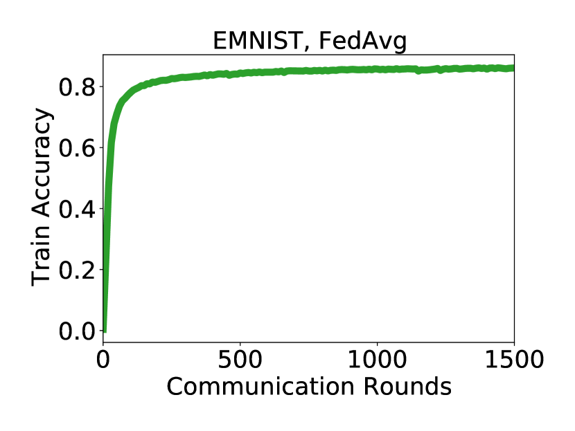
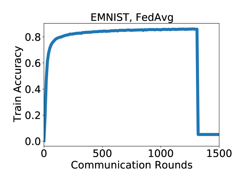
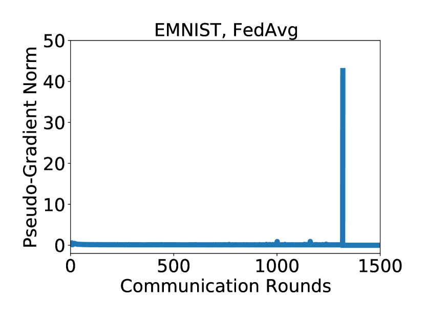
Figure 1: Applying FedAvg to EMNIST with cohort size $200$. We plot the train accuracy and norm of the pseudo-gradient for a trial that ran successfully (left), and one that experienced a catastrophic training failure (right). The trials differed only in which clients were randomly sampled each round.

The failure rate increased from 0% for $M=10$ to 80% for $M=800$. When failures occurred, we consistently saw a spike in the norm of the pseudo-gradient $\Delta$ (see Figure 1). In order to prevent this spike, we apply clipping to the client updates. We use the adaptive clipping method of (Andrew et al., 2019). While this technique was originally designed for training with differential privacy, we found that it greatly improved the stability of large-cohort training. Applying FedAvg to EMNIST with adaptive clipping, no catastrophic training failures occurred for any cohort size. We use adaptive clipping in all subsequent experiments. For more details, see Section A.3.

3.2 Diminishing Returns

In this section, we show that increasing $M$ in Algorithm 1 can lead to improved convergence, but that such improvements diminish with $M$. To demonstrate this, we plot the test accuracy of FedAvg and FedSGD across multiple tasks, for varying cohort sizes $M$ in Figure 2.

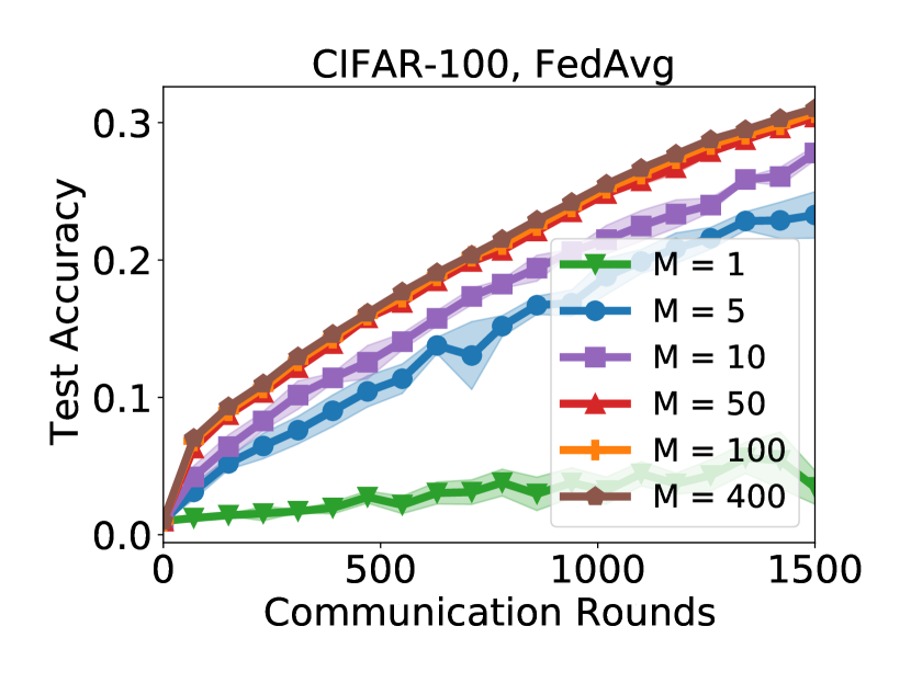
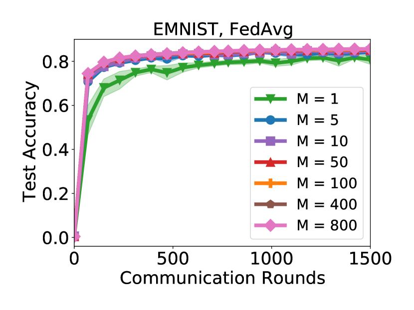
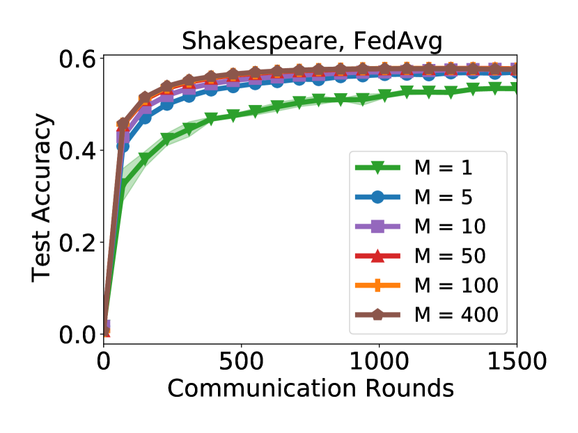
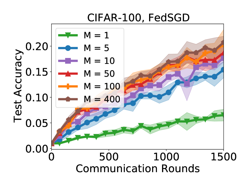
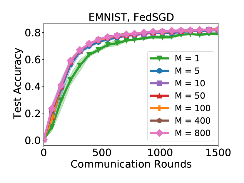
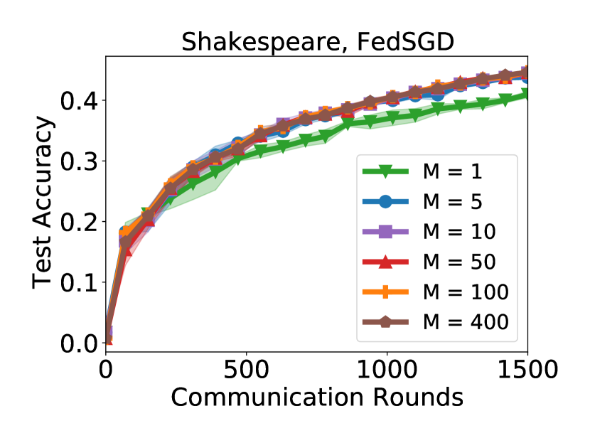
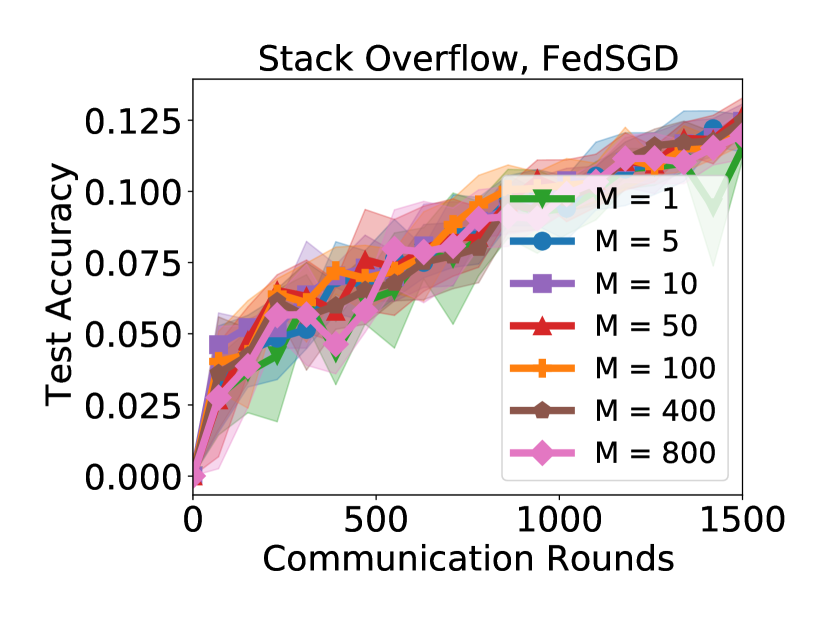
Figure 2: Test accuracy of FedAvg (top) and FedSGD (bottom), for various cohort sizes $M$, over the course of 1500 communication rounds.

We see that convergence benefits do not scale linearly with cohort size. While increasing $M$ from $1$ to $10$ can significantly improve convergence, there is generally a threshold after which point increasing $M$ incurs little to no change in convergence. This threshold is typically between $M=10$ and $M=50$. Interestingly, this seems to be true for both tasks, even though $M=50$ represents 10% of the training clients for CIFAR-10, but only approximately 0.015% of the training clients for Stack Overflow. We see comparable results for EMNIST and Shakespeare, as well as for other optimizers, including FedAdam and FedAdagrad. See Section B.1 for the full results. In short, we see that increasing $M$ alone can lead to diminishing returns, or even no returns in terms of convergence. This mirrors issues of diminishing returns in large-batch training (Dean et al., 2012; McCandlish et al., 2018; Golmant et al., 2018; Shallue et al., 2019).

In fact, such issues are not unique to FedAvg and FedSGD. More generally, we find that for all optimization methods we tried, the benefits of increasing the cohort size do not scale linearly. Instead, they saturate for large enough cohort sizes. To exemplify this, we plot the number of rounds needed by FedAvg and FedAdam to reach certain test accuracy thresholds in Figures 3 and 4. We see that while we see nearly linear speedups when increasing the cohort size from $M=1$ to a moderate value, we do not see linear speedups past this point. That being said, these figures demonstrate that large-cohort training does converge faster, and can reach accuracy values unobtainable by small cohort-training in communication-limited settings. For results for other optimizers, see Section B.3

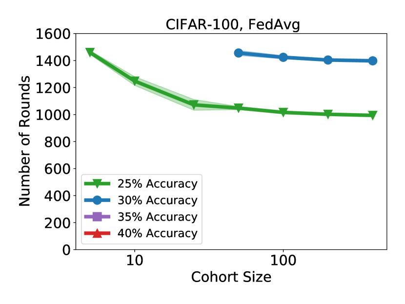
Figure 3: Number of communication rounds for FedAvg to obtain certain test accuracy thresholds. The $x$-axis denotes the cohort size.

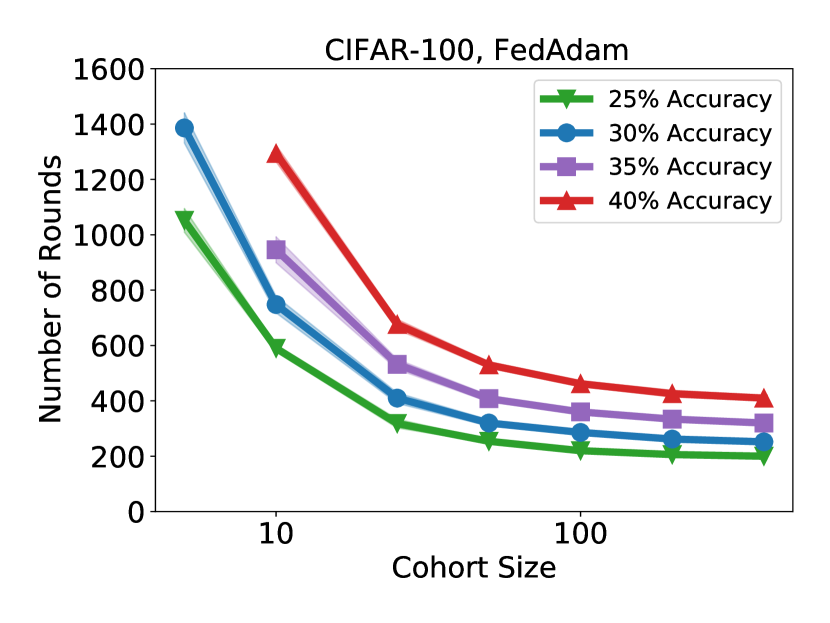
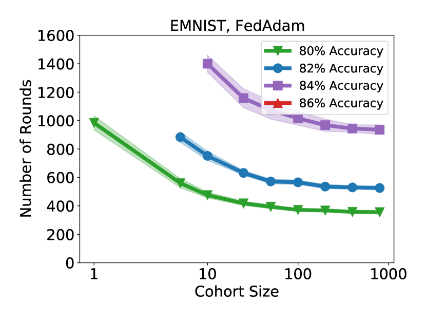
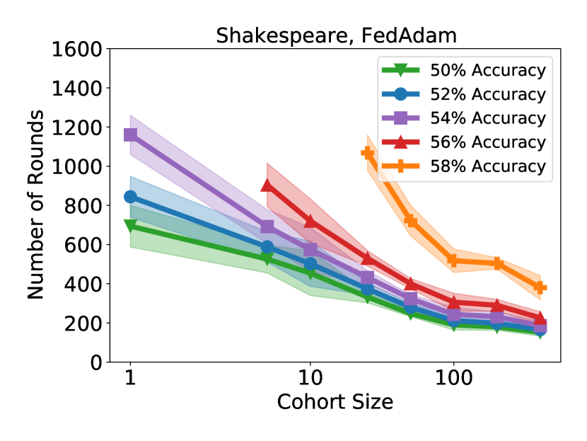
Figure 4: Number of communication rounds for FedAdam to obtain certain test accuracy thresholds. The $x$-axis denotes the cohort size.

3.3 Generalization Failures

Large-batch centralized optimization methods have repeatedly been shown to converge to models with worse generalization ability than models found by small-batch methods (Keskar et al., 2017; Hoffer et al., 2017; You et al., 2017; Masters and Luschi, 2018; Lin et al., 2019, 2020). Given the parallels between batch size in centralized learning and cohort size in FL, this raises obvious questions about whether similar issues occur in FL. In order to test this, we applied FedAvg, FedAdam, and FedAdagrad with different cohort sizes to various models. In Figure 5 we plot the train and test accuracy of our models after $T=1500$ communication rounds of FedAvg, FedAdam, and FedAdagrad.

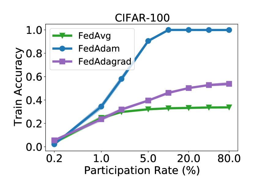
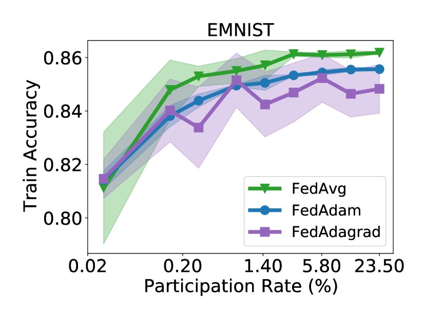
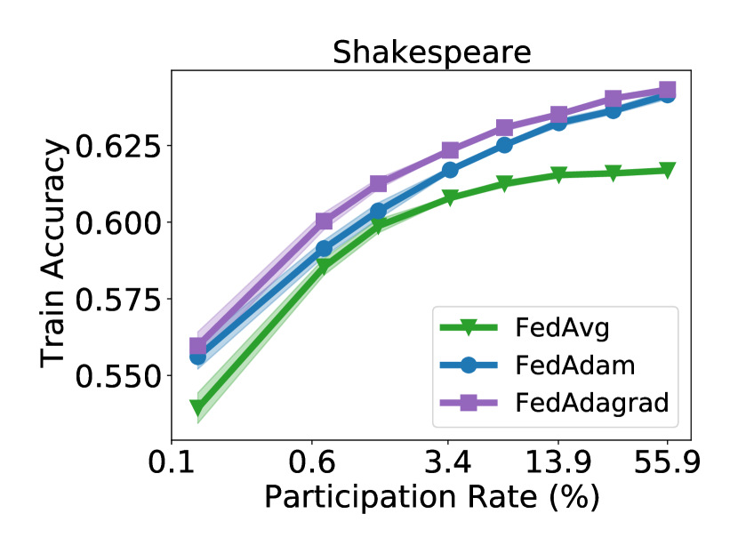
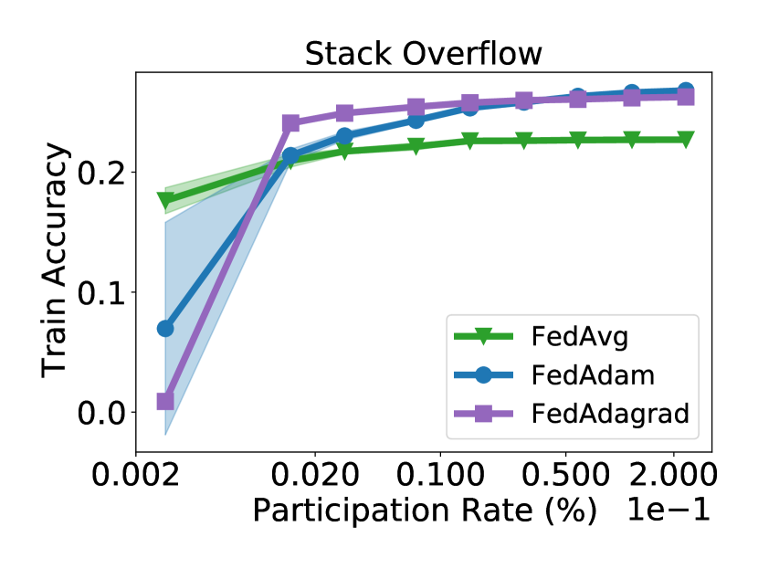
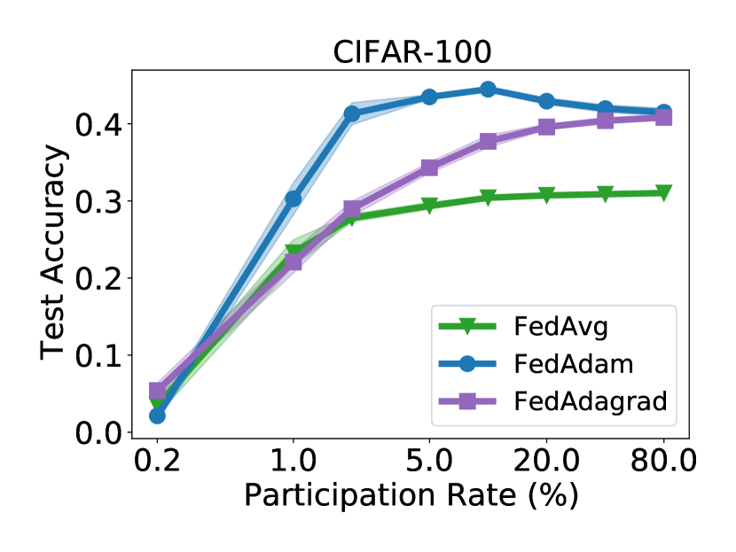
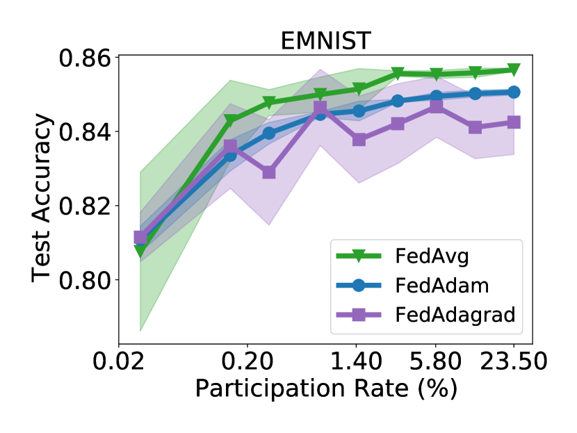
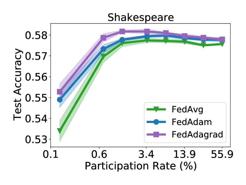
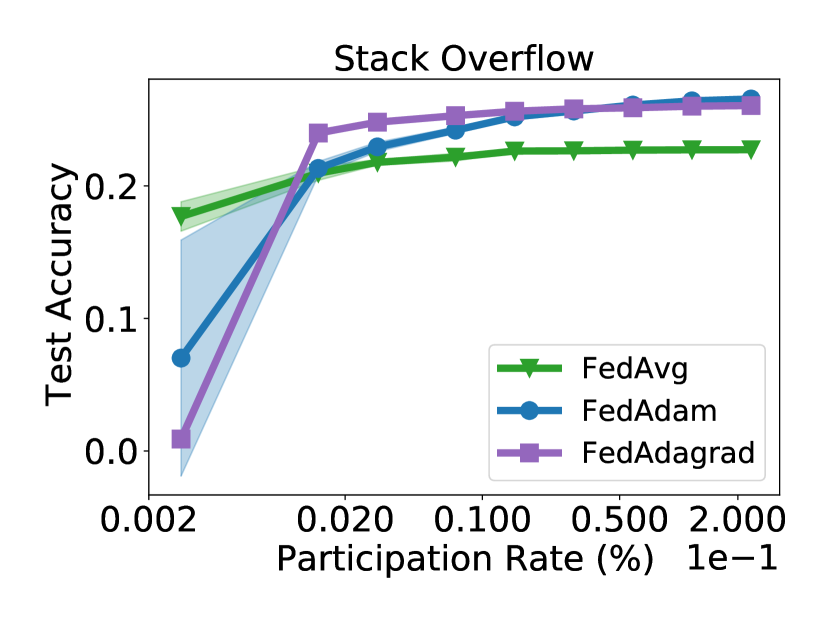
Figure 5: The train accuracy (top) and test accuracy (bottom) of FedAvg, FedAdam, and FedAdagrad on various tasks after training for 1500 communication rounds, for varying cohort sizes. The $x$-axis denotes the percentage of training clients in each cohort.

We find that generalization issues do occur in FL. For example, consider FedAdam on the CIFAR-100 task. While it attains roughly the same training accuracy for $M\in\{50,100,200,400\}$, we see that the larger cohorts uniformly lead to worse generalization. This resembles the findings of Keskar et al. (2017), who show that generalization issues of large-batch training can occur even though the methods reach similar training losses. However, generalization issues do not occur uniformly. It is often optimizer-dependent (as in CIFAR-100) and does not occur on the EMNIST and Stack Overflow datasets. Notably, CIFAR-100 and Shakespeare have many fewer clients overall. Thus, large-cohort training may reduce generalization, especially when the cohort size is large compared to the total number of clients.

3.4 Fairness Concerns

One critical issue in FL is fairness across clients, as minimizing (1) may disadvantage some clients (Mohri et al., 2019; Li et al., 2020c). Intuitively, large-cohort training methods may be better suited for ensuring fairness, since a greater fraction of the population is allowed to contribute to the model at each round. As a coarse measure of fairness, we compute percentiles of accuracy of our trained models across test clients. Fairer algorithms should lead to higher accuracy values for smaller percentiles. The percentiles for FedAdam on each task are given in Figure 6.

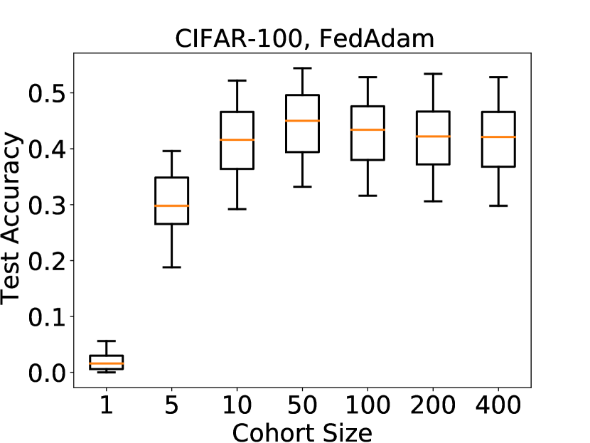
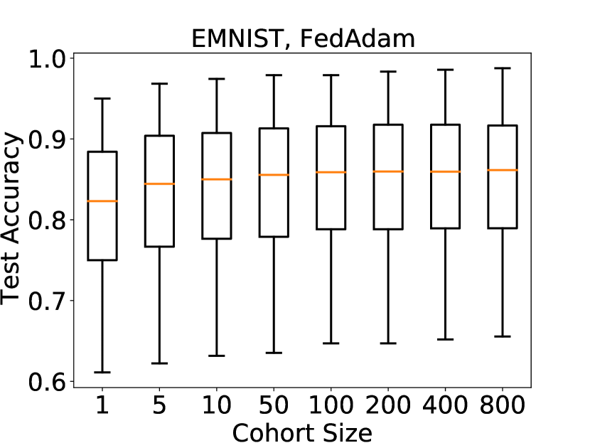
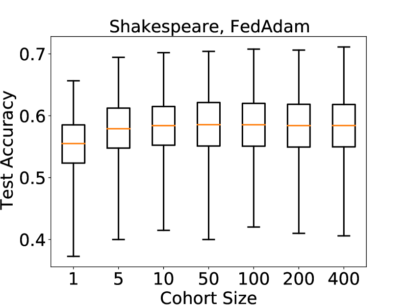
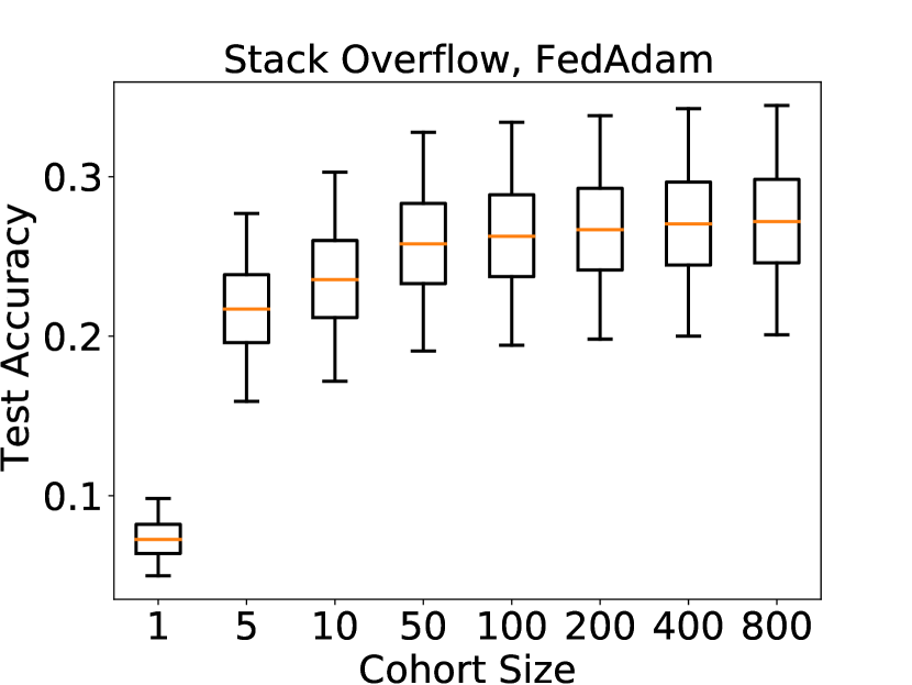
Figure 6: Accuracy of FedAdam after training for 1500 communication rounds using varying cohort sizes and tasks. The box plots show the 5th, 25th, 50th, 75th, and 95th percentiles of accuracy across test clients.

We find that the cohort size seems to affect all percentiles in the same manner. For example, on CIFAR-100, $M=50$ performs better for smaller percentiles and larger percentiles than larger $M$. This mirrors the CIFAR-100 generalization failures from Section 3.3. By contrast, for Stack Overflow we see increases in all percentiles as we increase $M$. While the accuracy gains are only slight, they are consistent across percentiles. This suggests a connection between the fairness of a federated training algorithm and the fraction of test clients participating at every round. Notably, increasing $M$ seems to have little effect on the spread between percentiles (such as the difference between the 75th and 25th percentiles) beyond a certain point. See Section B.4 for more results.

3.5 Decreased Data Efficiency

Despite issues such as diminishing returns and generalization failures, federated optimization methods can see some benefit from larger cohorts. Large-cohort training, especially with adaptive optimizers, often leads to faster convergence to given accuracy thresholds. For example, in Figure 7, we see that the number of rounds FedAdam requires to reach certain accuracy thresholds generally decreases with the cohort size.

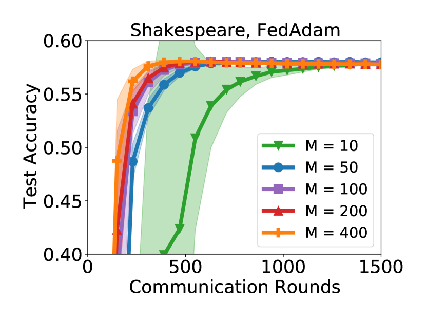
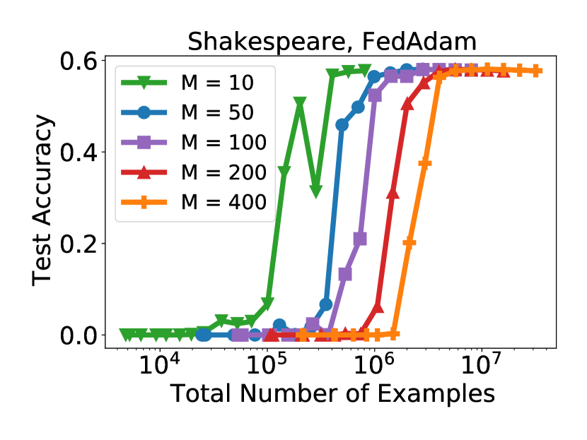
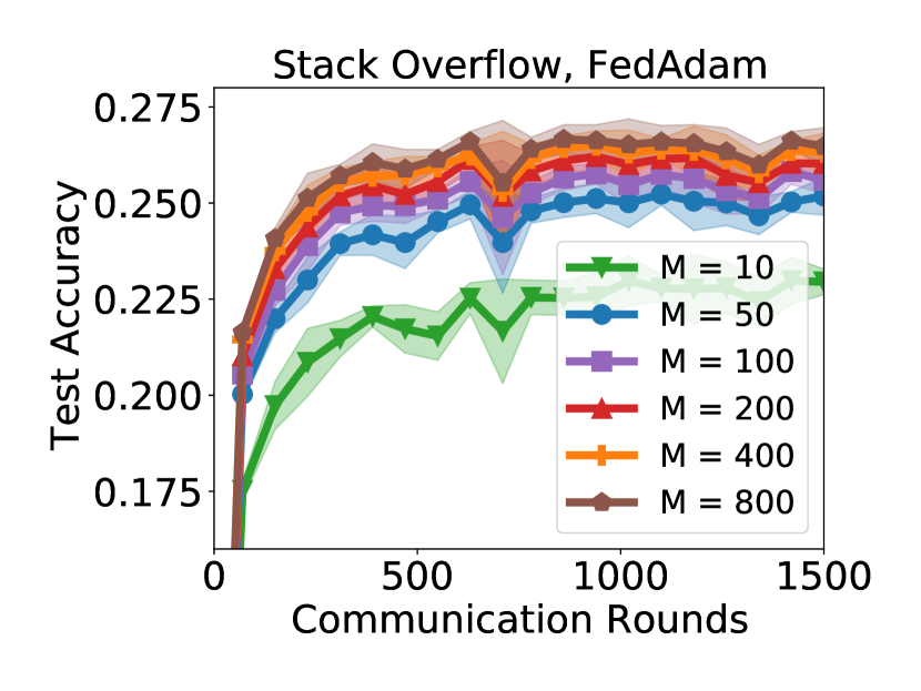
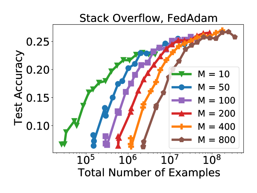
Figure 7: Test accuracy of FedAdam on Shakespeare (left) and Stack Overflow (right) with various cohort sizes. We plot versus the number of communication rounds and the number of examples processed in total.

While it is tempting to say that large-cohort methods are “faster”, this ignores the practical costs of large-cohort training. Completing a single communication round often requires more resources with larger cohorts. To showcase this, we also plot the accuracy of FedAdam with respect to the number of examples seen in Figure 7. This measures the data-efficiency of large-cohort training, and shows that large cohort-training requires significantly more examples per unit-accuracy.

While data-inefficiency also occurs in large-batch training (McCandlish et al., 2018), it is especially important in federated learning. Large-cohort training faces greater limitations on parallelizability due to data-sharing constraints. Worse, in realistic cross-device settings client compute times can scale super-linearly with their amount of data, so clients with more data are more likely to become stragglers (Bonawitz et al., 2019). This straggler effect means that data-inefficient algorithms may require longer training times. To demonstrate this, we show in Section B.5 that under the probabilistic straggler runtime model from (Lee et al., 2017), large-cohort training can require significantly more compute time to converge.

4 Diagnosing Large-Cohort Challenges

We now examine the challenges in Section 3, and provide partial explanations for their occurrence. One of the key differences between FedAvg and FedSGD is what the pseudo-gradient $\Delta$ in (1) represents. In FedSGD, $\Delta$ is a stochastic gradient estimate (i.e., $\mathbb{E}[\Delta]=\nabla f$, where the expectation is over all randomness in a given communication round). For special cases of Algorithm 1 where clients perform multiple local training steps, $\Delta$ is not an unbiased estimator of $\nabla f$ (Malinovskiy et al., 2020; Pathak and Wainwright, 2020; Charles and Konečný, 2021). While increasing the cohort size should reduce the variance of $\Delta$ as an estimator of $\mathbb{E}[\Delta]$, it is unclear what this quantity represents.

To better understand $\Delta$, we plot its norm on Stack Overflow in Figures 8(a) and 8(b). For FedSGD, $\|\Delta\|$ decreases slightly with $M$, but has high variance. By contrast, for FedAvg larger cohorts lead to smaller norms with little overlap. The decrease in norm obeys an inverse square root rule: Let $\Delta_{1},\Delta_{2}$ be pseudo-gradients at some round for cohort sizes $M_{1},M_{2}$. For FedAvg, $\|\Delta_{1}\|/\|\Delta_{2}\|\approx\sqrt{M_{2}/M_{1}}$. We use this rule to predict pseudo-gradient norms for FedAvg in Figure 8(c). After a small number of rounds, we obtain a remarkably good approximation. To explain this, we plot the average cosine similarity between client updates $\Delta_{k}^{t}$ at each round in Figure 8(d), with $M=50$. For FedAvg, the client updates are on average almost orthogonal. This explains Figure 8(b), as $\Delta$ is an average of nearly orthogonal vectors. As we show in Section B.6, similar results hold for other tasks and optimizers.

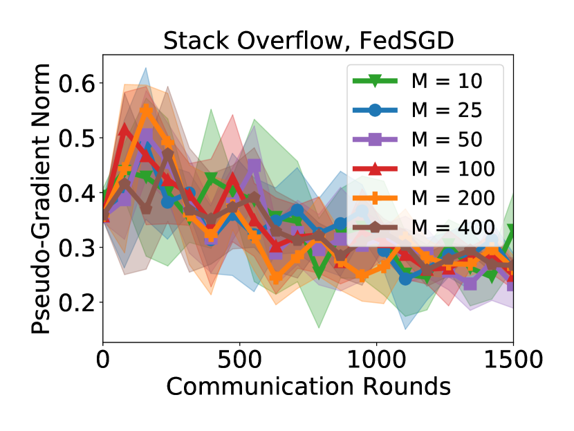
(a)

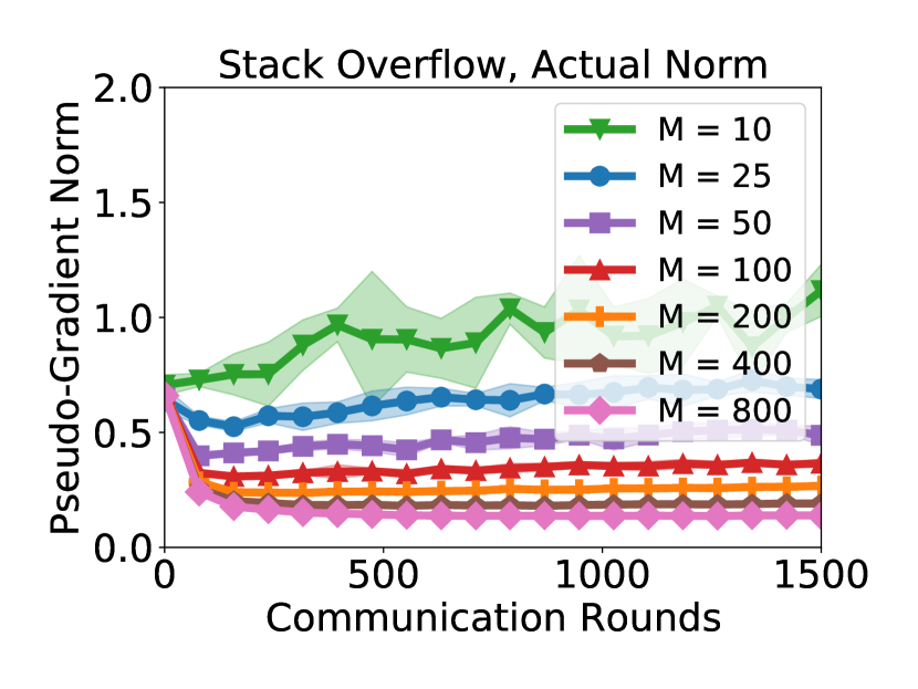
(b)

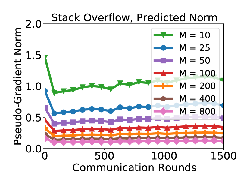
(c)

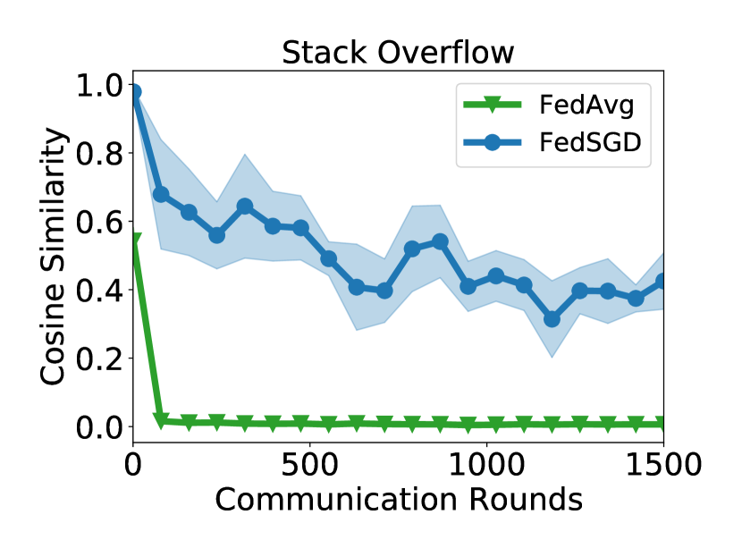
(d)

Figure 8: The pseudo-gradient norm of FedSGD (a) and FedAvg (b) on Stack Overflow with varying cohort sizes $M$. We also plot the predicted norm for FedAvg using an inverse square root scaling rule relative to $M=50$ (c) and the average cosine similarity of client updates for $M=50$ (d).

Implications for large-cohort training. This near-orthogonality of client updates is key to understanding the challenges in Section 3. The diminishing returns in Section 3.2 occur in part because increasing $M$ leads to smaller updates. This also sheds light on Section 3.5: In large-cohort training, we take an average of many nearly-orthogonal vectors, so each client’s examples contribute little. The decreasing pseudo-gradient norms in Figure 8(c) also highlights an advantage of methods such as FedAdam and FedAdagrad: Adaptive server optimizers employ a form of normalization that makes them somewhat scale-invariant, compensating for this norm reduction.

5 Designing Better Methods

We now explore an initial set of approaches aimed at improving large-cohort training, drawing inspiration where possible from large-batch training. Our solutions are designed to provide simple baselines for improving large-cohort training. In particular, our methods and experiments are intended to serve as a useful reference for future work in the area, not to fully solve the challenges of large-cohort training.

5.1 Learning Rate Scaling

One common technique for large-batch training is to scale the learning rate according to the batch size. Two popular scaling methods are square root scaling (Krizhevsky, 2014) and linear scaling (Goyal et al., 2017). While such techniques have had clear empirical benefit in centralized training, there are many different ways that they could be adapted to federated learning. For example, in Algorithm 1, the client and server optimization both use learning rates that could be scaled.

We consider the following scaling method for large-cohort training: We fix the client learning rate, and scale the server learning rate with the cohort size. Such scaling may improve convergence by compensating for the pseudo-gradient norm reduction in Figure 8. We use square root and linear scaling rules: Given a learning rate $\eta_{s}$ tuned for $M$, for $M^{\prime}\geq M$ we use a learning rate $\eta_{s}^{\prime}$ where

$$\eta_{s}^{\prime}=\frac{\sqrt{M^{\prime}}}{\sqrt{M}}\eta_{s}\text{ (square root scaling)~{}~{}~{}OR~{}~{}~{}}\eta_{s}^{\prime}=\frac{M^{\prime}}{M}\eta_{s}\text{ (linear scaling)}.$$ (3)

We also use a version of the warmup strategy from (Goyal et al., 2017). For the first $W$ communication rounds, we linearly increase the server learning rate from $\eta_{s}$ to $\eta_{s}^{\prime}$. In our experiments, we set $W=100$ and use a reference server learning rate $\eta_{s}$ tuned for $M=50$.

Our experiments show that server learning rate scaling rules have mixed efficacy in large-cohort training. Linear scaling is often too aggressive for federated learning, and caused catastrophic training failures beyond $M=100$ even when using adaptive clipping. As we show in Section B.7, when applying FedAvg to EMNIST with the linear scaling rule, we found that catastrophic failures occurred for $M>100$, with no real improvement in accuracy for $M=100$.

By contrast, square root scaling did not cause catastrophic training failures. We plot the train and test accuracy of FedAvg using square root scaling in Figure 9. As we see, the performance varied across tasks. While it improved both train and test accuracy for CIFAR-100, for Shakespeare it improved train accuracy while reducing test accuracy. While we saw small improvements in accuracy for some cohort sizes on EMNIST and Stack Overflow, it degraded accuracy for the largest cohort sizes. In sum, we find that applying learning rate scaling at the server may not directly improve large-cohort training.

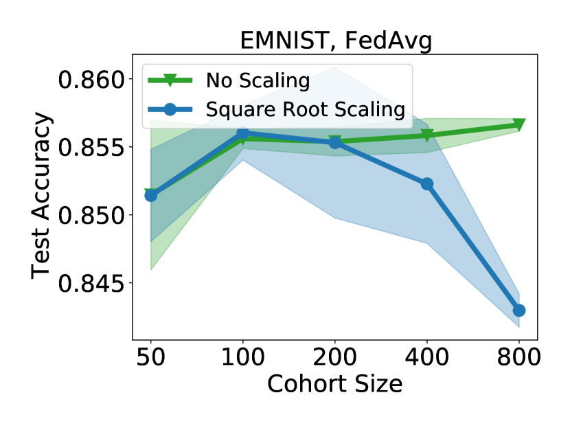
Figure 9: The train accuracy (top) and test accuracy (bottom) of FedAvg using square root scaling with warmup, versus no scaling. Results are recorded after 1500 rounds, for varying cohort sizes.

5.2 Layer-wise Adaptivity

Another popular technique for large-batch training is layer-wise adaptivity. Methods such as LARS (You et al., 2017) and Lamb (You et al., 2020) use layer-wise adaptive learning rates, which may allow the methods to train faster than SGD with linear scaling and warmup in large-batch settings (You et al., 2017, 2020). We propose two new federated versions of these optimizers, FedLARS and FedLamb. These are special cases of Algorithm 1, where the server uses LARS and Lamb, respectively. Given the difficulties of learning rate scaling above, FedLARS and FedLamb may perform better in large-cohort settings.

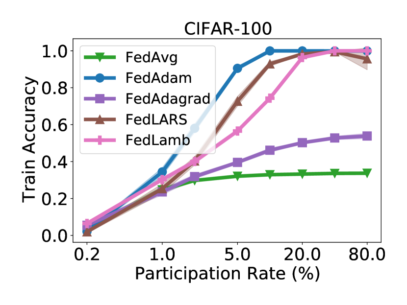
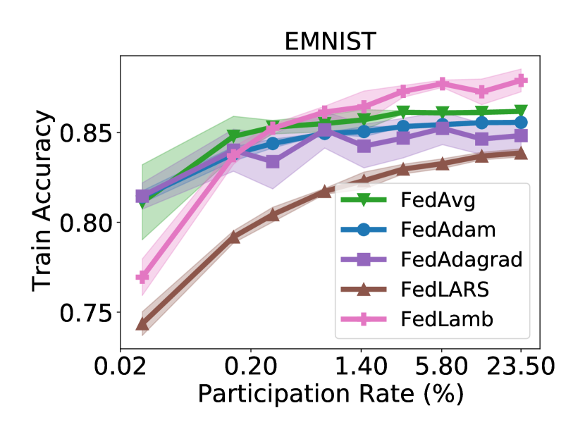
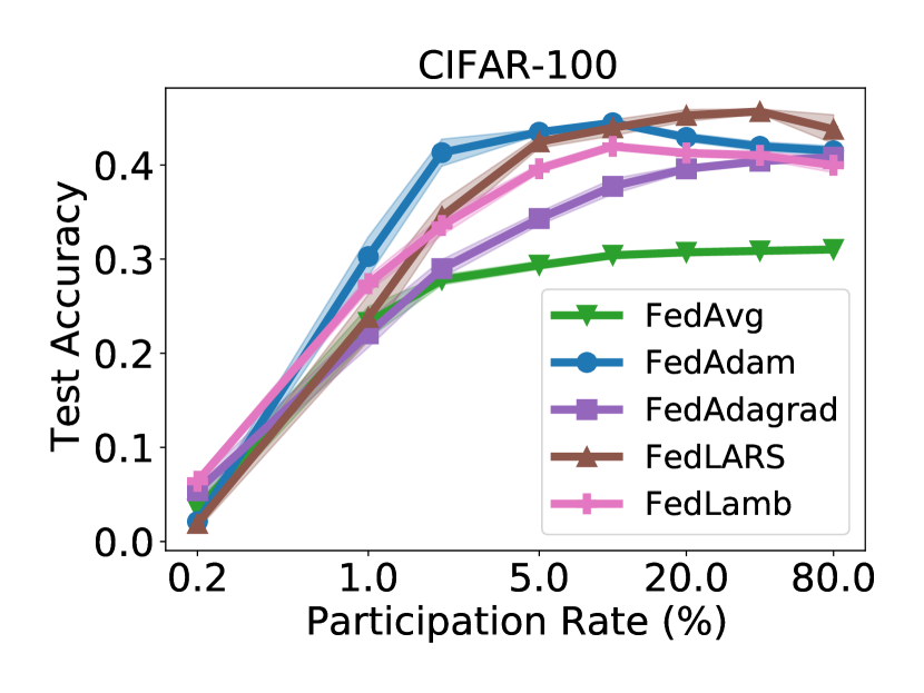
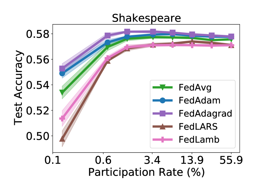
Figure 10: The train accuracy (top) and test accuracy (bottom) of various methods, including FedLARS and FedLamb, after training for 1500 rounds, for varying cohort sizes and on varying tasks. The $x$-axis denotes percentage of training clients in each cohort.

In Figure 10 we present the train and test accuracy of various methods, including FedLARS and FedLamb, for varying cohort sizes. In most cases, we see that FedLamb performs comparably to FedAdam for large cohort sizes, but with slightly worse performance in intermediate stages. One notable exception is Stack Overflow, in which FedLamb performs well even for $M=1$. As in Section 3.3, FedLamb sees an eventual drop in test accuracy for $M>100$. FedLARS has decidedly mixed performance. While it performs well on CIFAR-10, it does not do well on EMNIST or Shakespeare. While federated layer-wise adaptive algorithms can be better than coordinate-wise adaptive algorithms on certain datasets in some large-cohort settings, our results do not indicate that they are universally better.

5.3 Dynamic Cohort Sizes

As we saw in Section 3.5, large-cohort training can reduce data efficiency. Part of this stems from the fact that larger cohorts may help very little for smaller accuracy thresholds (see Figure 7). In order to improve data efficiency, we may be able to use smaller cohorts in earlier optimization stages, and increase the cohort size over time. This technique is parallel to “dynamic batch size” techniques used in large-batch training (Smith et al., 2018). In order to test the efficacy of such techniques in large-cohort training, we start with an initial cohort size of $M=50$ and double the size every 300 rounds up to $M=800$ (or the maximum population size if smaller). This results in doubling the cohort size a maximum of 4 times over the $1500$ rounds of training we perform. We plot the results for FedAvg and FedAdam on CIFAR-100 and Stack Overflow in Figure 11. See Section B.8 for results on all tasks.

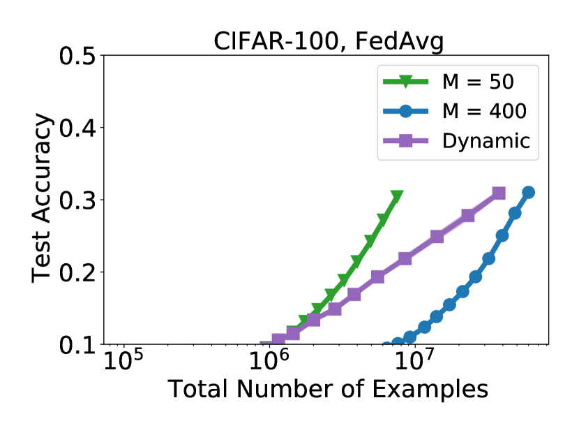
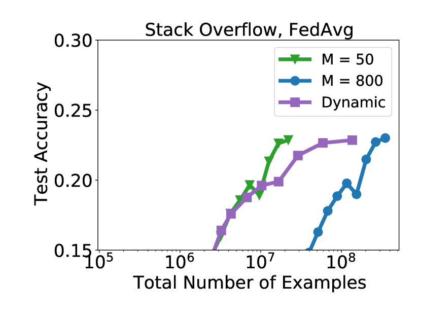
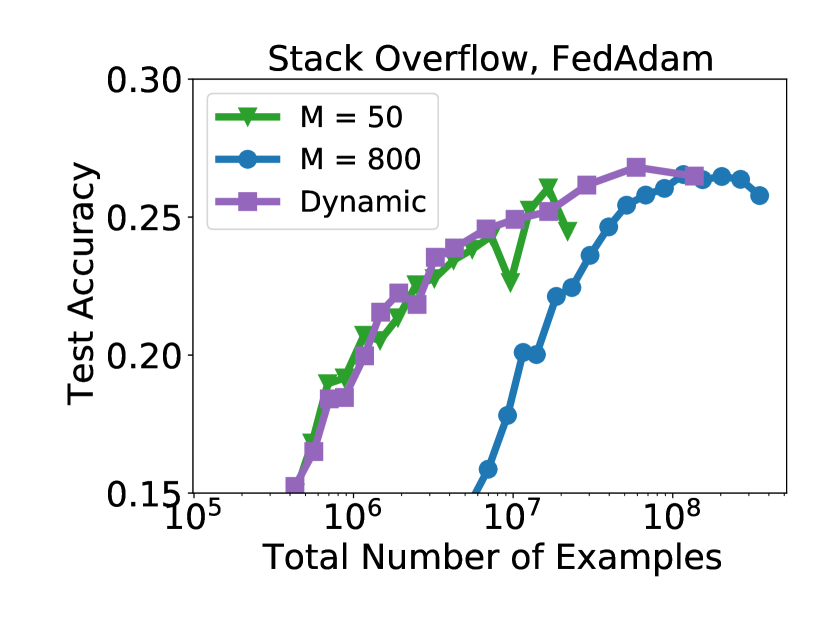
Figure 11: Test accuracy of FedAvg and FedAdam on Shakespeare (left) and Stack Overflow (right), with respect to the total number of examples processed, using fixed and dynamic cohort sizes.

This dynamic strategy attains data efficiency closer to a fixed cohort size of $M=50$, while still obtaining a final accuracy closer to having used a large fixed cohort size. While our initial findings are promising, we note two important limitations. First, the accuracy of the dynamic strategy is bounded by the minimum and maximum cohort size used; It never attains a better accuracy than $M=800$. Second, the doubling strategy still faces the generalization issues discussed in Section 3.3.

5.4 Normalized FedAvg

While the methods above show promise in resolving some of the issues of large-cohort training, they also introduce extra hyperparameters (such as what type of learning rate scaling to use, or how often to double the cohort size). Notably, hyperparameter tuning can be difficult in federated learning, especially cross-device federated learning (Kairouz et al., 2021). Even adaptive methods like FedAdam introduce a number of new hyperparameters that can be challenging to contend with. We are therefore motivated to design a large-cohort training method that does not introduce any new hyperparameters.

Recall that in Section 4, we showed that for FedAvg, the client updates ($\Delta_{k}^{t}$ in Algorithm 1 and Algorithm 2) are nearly orthogonal in expectation. By averaging nearly orthogonal updates in large-cohort training, we get a server pseudo-gradient $\Delta^{t}$ that is close to zero, meaning that the server does not make much progress at each communication round. In order to compensate for this without having to tune a learning rate scaling strategy, we propose a simple variant of FedAvg that tries to account for this near-orthogonality of client updates. Rather than applying SGD to the server pseudo-gradient (as in Algorithm 1), we apply SGD to the normalized server pseudo-gradient. That is, the server updates its model via

$$x^{\prime}=x-\eta_{s}\frac{\Delta}{\|\Delta\|_{2}}.$$

This is a kind of federated analog of normalized SGD methods used for centralized learning (Nacson et al., 2019). It introduces no new hyperparameters with respect to Algorithm 1. To test this method, which we refer to as normalized FedAvg, we present its training and test accuracy versus cohort size in Figure 12. Notably, we do not re-tune any learning rates. We simply use the same learning rates tuned for (unnormalized) FedAvg.

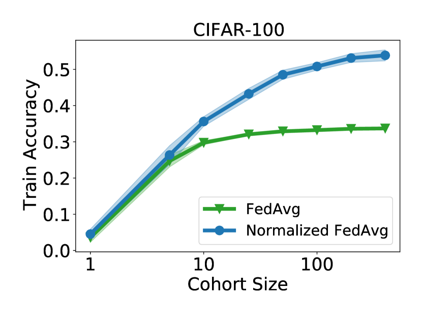
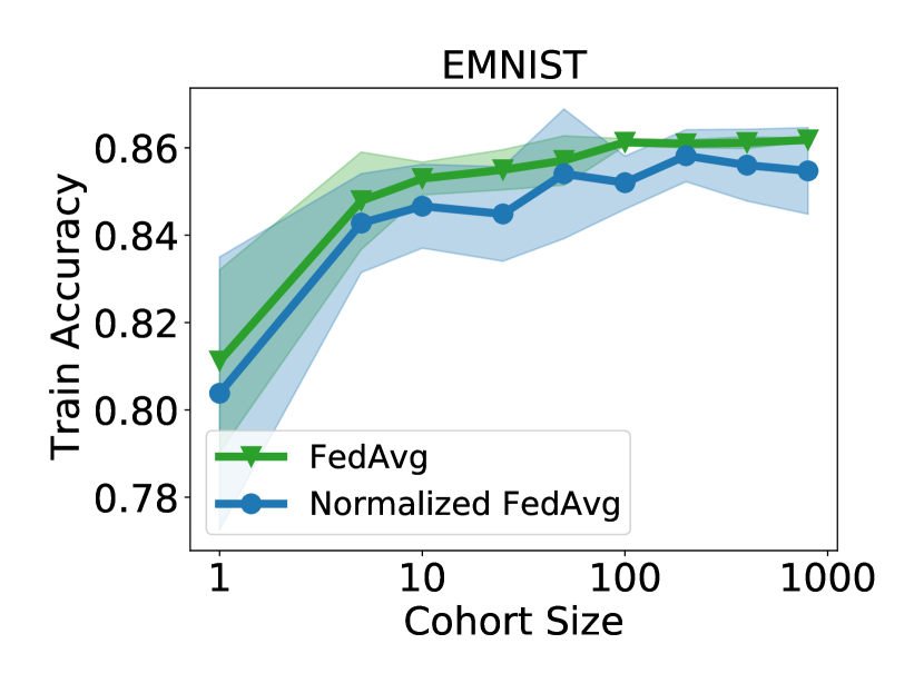
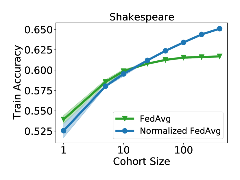
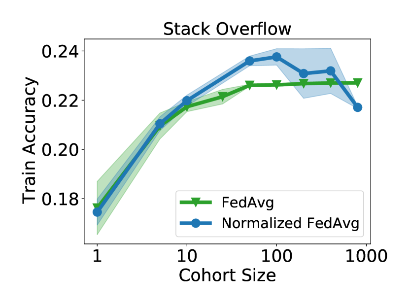
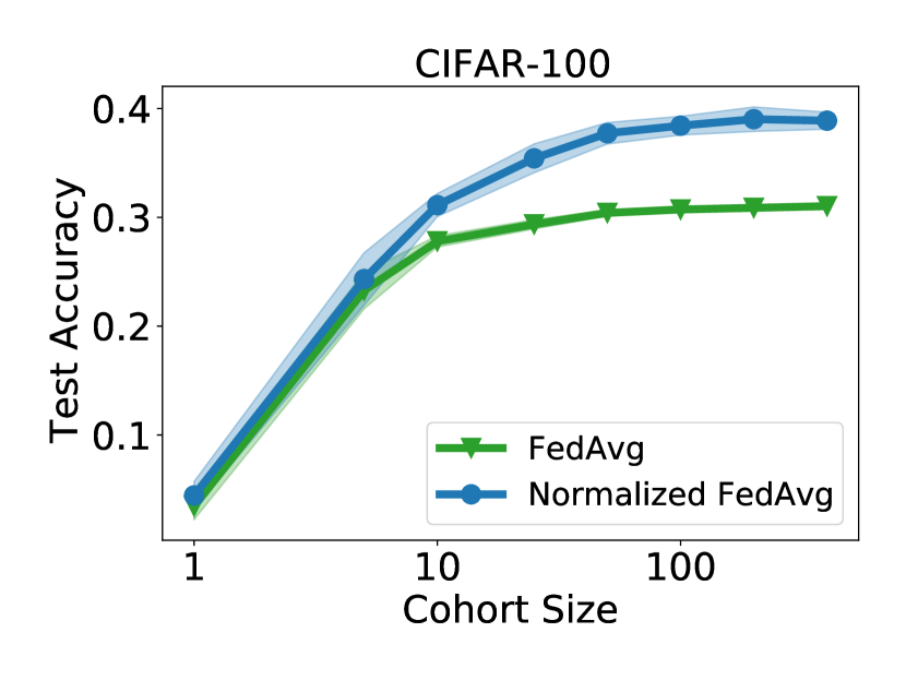
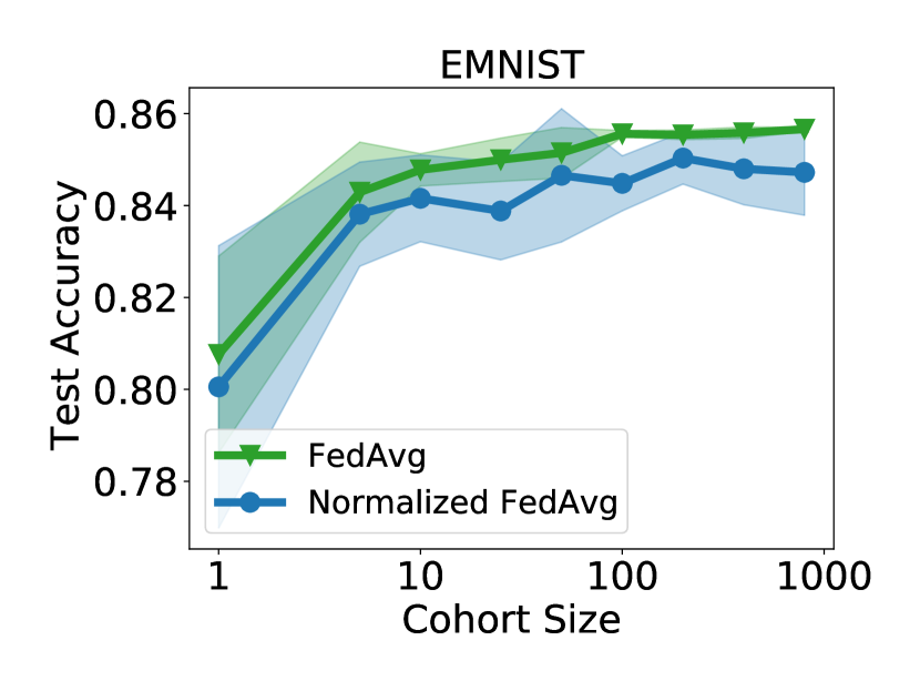
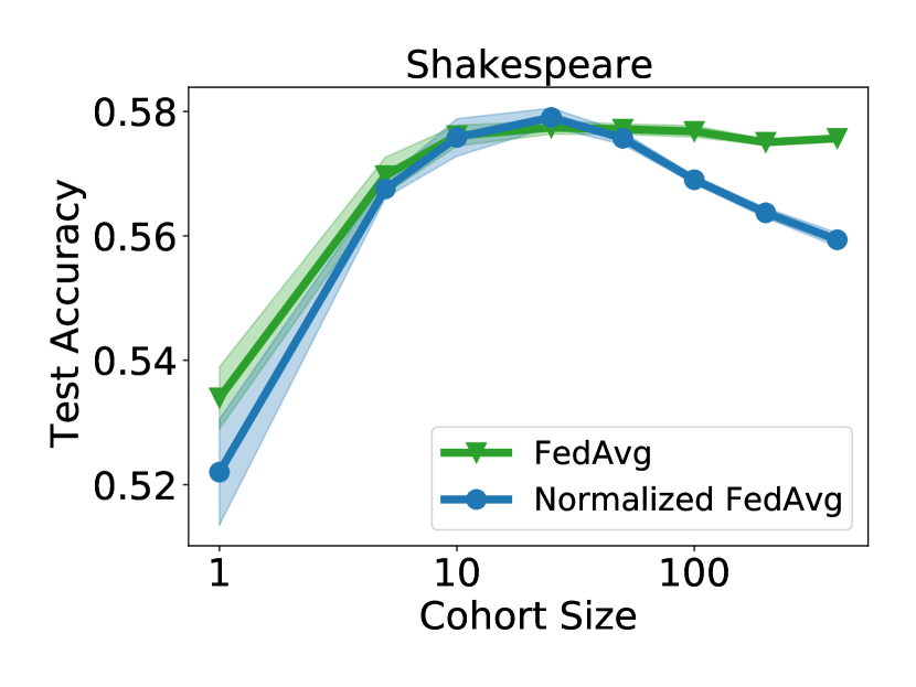
Figure 12: The train accuracy (top) and test accuracy (bottom) of FedAvg and the normalized variant of FedAvg, after training for 1500 communication rounds. Results are given for various cohort sizes and tasks

We find that for most cohort sizes and on most tasks, normalized FedAvg achieves better training accuracy for larger cohorts. Thus, this helps mitigate the diminishing returns issue in Section 3.2. We note two important exceptions: for EMNIST, the normalized FedAvg is slightly worse for all cohort sizes. For Stack Overflow, it obtains worse training accuracy for the largest cohort size. However, we see significant improvements on CIFAR-100 and all but the largest cohort sizes for Stack Overflow. We believe that the method therefore exhibits promising results, and may be improved in future work.

5.5 Changing the Number of Local Steps

While the cohort size has clear parallels to batch size, it is not the only factor determining the number of examples seen per round in Algorithm 1. The number of client epochs $E$ and the client batch size also affect this. To study this “effective batch size” in FL, we fix the client batch size, and investigate how the cohort size and number of local steps simultaneously impact the performance of FedAvg.

In particular, we fix a local batch size of $1$ and vary the cohort size over $\{16,32,\dots,1024\}$. We vary the number of local steps over $\{1,2,4,\dots,256\}$. We plot the number of rounds needed for convergence, and the final test accuracy in Figure 13. By construction, each square on an anti-diagonal corresponds to the same number of examples per round.

In the left figure, we see that if we fix the cohort size, then increasing the number of local steps can accelerate convergence, but only up to a point, after which catastrophic training failures occur. By contrast, if we have convergence for some number of local steps and cohort size, convergence occurs for all cohort sizes. Similarly, we see in the right hand figure that increasing the number of local steps can drastically reduce generalization, more so than increasing the cohort size. In essence, we see that the number of local steps obeys many of the same issues outlined in Section 3. Therefore, correctly tuning the number of local steps in unison with the cohort size may be critical to ensuring good performance of large-cohort methods.

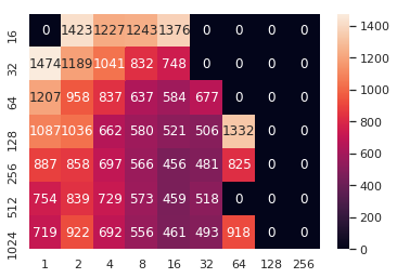
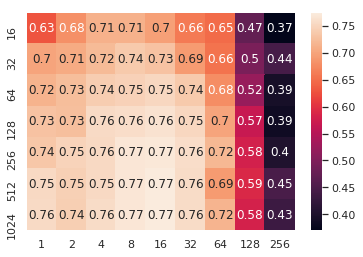
Figure 13: The number of rounds for to reach a test accuracy of $70\%$ (left) and the test accuracy after 1500 rounds (right). Results are for FedAvg on EMNIST with varying numbers of local steps ($x$-axis) and cohort sizes ($y$-axis).

6 Limitations and Future Work

In this work we explore the benefits and limitations of large-cohort training in federated learning. As discussed in Sections 3.5 and 5, focusing on the number of communication rounds often obscures the data efficiency of a method. This in turn impacts many metrics important to society, such as total energy consumption or total carbon emissions. While we show that large-cohort training can negatively impact such metrics by reducing data-efficiency (see Section 3.5 and Section B.5), a more specialized focus on these issues is warranted. Similarly, we believe that an analysis of fairness in large-cohort settings going beyond Section 3.3 would be beneficial.

Future work also involves connecting large-cohort training to other important aspects of federated learning, and continuing to explore connections with growing lines of work in large-batch training. In particular, we wish to see whether noising strategies, especially differential privacy mechanisms, can help overcome the generalization issues of large-cohort training. Personalization may also help mitigate issues of generalization and fairness. Finally, although not a focus of our work, we note that some of the findings above may extend to cross-silo settings, especially if communication restrictions require subsampling clients.

Appendix A Full Experimental Details

A.1 Datasets and Models

We use four datasets throughout our work: CIFAR-100 (Krizhevsky, 2009), the federated extended MNIST dataset (EMNIST) (Cohen et al., 2017), the Shakespeare dataset (Caldas et al., 2018), and the Stack Overflow dataset (Authors, 2019a). The first two datasets are image datasets, the second two are language datasets. All datasets are publicly available. We specifically use the versions available in TensorFlow Federated (Authors, 2019b), which gives a federated structure to all four datasets. Below we discuss the specifics of the dataset and classification task, as well as the model used to perform classification.

CIFAR-100

The CIFAR-100 dataset is a computer vision dataset consisting of $32\times 32\times 3$ images with 100 possible labels. While this dataset does not have a natural partition among clients, a federated version was created by Reddi et al. (2021) using hierarchical latent Dirichlet allocation to enforce moderate amounts of heterogeneity among clients. This partitioning among clients was based on Pachinko allocation (Li and McCallum, 2006). Note that under this partitioning, each client typically has only a subset of the 100 possible labels. The dataset has 500 training clients and 100 test clients, each with 100 examples in their local dataset.

We train a ResNet-18 (He et al., 2016) on this dataset, where we replace all batch normalization layers with group normalization layers (Wu and He, 2018). The use of group norm over batch norm in federated learning was first advocated by Hsieh et al. (2020), who showed that this helped improve classification accuracy in the presence of heterogeneous clients. We specifically use group normalization layers with two groups. We perform small amounts of data augmentation and preprocessing for each train and test sample. We first centrally crop each image $(24,24,3)$. We then normalize the pixel values according to their mean and standard deviation.

EMNIST

The EMNIST dataset consists of images hand-written alphanumeric characters. Each image consists of $28\times 28$ gray-scale pixel values. There are 62 total alphanumeric characters represented in the dataset. The images are partitioned among clients according to their author. The dataset has 3,400 clients, who have both train and test datasets. The dataset has natural heterogeneity stemming from the writing style of each person. We train a convolutional network on the dataset (the same one used by Reddi et al. (2021)). The network uses two convolutional layers (each with $3\times 3$ kernels and strides of length 1), followed by a max pooling layer using dropout with $p=0.25$, a dense layer with 128 units and dropout with $p=0.5$, and a final dense output layer.

Shakespeare

The Shakespeare dataset is derived from the benchmark designed by Caldas et al. (2018). The dataset corpus is the collected works of William Shakespeare, and the clients correspond to roles in Shakespeare’s plays with at least two lines of dialogue. To eliminate confusion, character here will refer to alphanumeric characters (such as the letter q) and symbols such as punctuation, while we will use client to denote the various roles in plays (such as Macbeth). There are a total of 715 clients, whose lines are partitioned between train and test datasets.

We split each client’s lines into sequences of 80 characters, padding if necessary. We use a vocabulary size of 90, where 86 characters are contained in Shakespeare’s work, and the remaining 4 are beginning and end of line tokens, padding tokens, and out-of-vocabulary tokens. We perform next-character prediction on the clients’ dialogue using a recurrent neural network (RNN) (Mikolov et al., 2010). We use the same model as Reddi et al. (2021). The RNN takes as input a sequence of 80 characters, embeds it into a learned 8-dimensional space, and passes the embedding through 2 LSTM layers (Hochreiter and Schmidhuber, 1997), each with 256 units. Finally, we use a softmax output layer with 80 units, where we try to predict a sequence of 80 characters formed by shifting the input sequence over by one. Therefore, our output dimension is $80\times 90$. We compute loss using cross-entropy loss.

Stack Overflow

Stack Overflow is a language dataset consisting of question and answers from the Stack Overflow site. The questions and answers also have associated metadata, including tags. Each client corresponds to a user. The specific train/validation/test split from (Authors, 2019a) has 342,477 train clients, 38,758 validation clients, and 204,088 test clients. Notably, the train clients only have examples from before 2018-01-01 UTC, while the test clients only have examples from after 2018-01-01 UTC. The validation clients have examples with no date restrictions, and all validation examples are held-out from both the test and train sets.

We perform next-word prediction on this dataset. We restrict each client to the first 1000 sentences in their dataset (if they contain this many, otherwise we use the full dataset). We also perform padding and truncation to ensure that each sentence has 20 words. We then represent the sentence as a sequence of indices corresponding to the 10,000 most frequently used words, as well as indices representing padding, out-of-vocabulary words, the beginning of a sentence, and the end of a sentence. We perform next-word-prediction on these sequences using an a recurrent neural network (RNN) (Mikolov et al., 2010) that embeds each word in a sentence into a learned 96-dimensional space. It then feeds the embedded words into a single LSTM layer (Hochreiter and Schmidhuber, 1997) of hidden dimension 670, followed by a densely connected softmax output layer. Note that this is the same model used by Reddi et al. (2021). The metric used in the main body is the accuracy over the 10,000-word vocabulary; it does not include padding, out-of-vocab, or beginning or end of sentence tokens when computing the accuracy.

A.2 Implementation and Hyperparameters

We implement the previously proposed methods of FedAvg, FedSGD, FedAvgM, FedAdam, FedAdagrad, as well as two novel methods, FedLARS and FedLamb. All implementations are special cases of Algorithm 1. In all cases, clients use mini-batch SGD with batch size $B$. For FedSGD, the batch size $B$ of a client is set to the size of its local dataset (so that the client only takes a single step). For all other optimizers, we fix $B$ at a per-task level (see Table 2). Note that we use larger batch sizes for datasets where clients have more examples, like Stack Overflow. Except for the experiments in Section 5.5, we set $E=1$ throughout.

Table 2: Batch sizes used for each for all algorithms (except for FedSGD) on each dataset.

Dataset	Batch Size
CIFAR-100	20
EMNIST	20
Shakespeare	4
Stack Overflow	32

For the actual implementation of the algorithms above, all methods (except for FedSGD) differ only in the choice of ServerOpt in Algorithm 1. For FedSGD, in addition to having clients use full-batch SGD (as mentioned above), the client learning rate is set to be $\eta_{c}=1$ in order to allow Algorithm 1 to recover the version of FedSGD proposed by McMahan et al. (2017). For all other algorithms, we present the choice of ServerOpt and relevant hyperparameters (except for learning rates, see Section A.4) in Table 3. Note that here we use the notation from (Kingma and Ba, 2015), where $\beta_{1}$ refers to a first-moment momentum parameter, $\beta_{2}$ refers to a second-moment momentum parameter, and $\epsilon$ is a numerical stability constant used in adaptive methods. Note that for all adaptive methods, we set their initial accumulators to be 0.

Table 3: Hyperparameters and implementation details for all algorithms, relative to Algorithm 1. Here, $\beta_{1}$ denotes a first-moment momentum parameter, $\beta_{2}$ denotes a second-moment momentum parameter, and $\epsilon$ is a value used for numerical stability purposes in adaptive methods.

Algorithm	ServerOpt	$\beta_{1}$	$\beta_{2}$	$\epsilon$
FedAvg (McMahan et al., 2017)	SGD	0	N/A	N/A
FedAvgM (Hsieh et al., 2020)	SGD	0.9	N/A	N/A
FedAdagrad (Reddi et al., 2021)	Adagrad (Duchi et al., 2011)	N/A	N/A	0.001
FedAdam (Reddi et al., 2021)	Adam (Kingma and Ba, 2015)	0.9	0.99	0.001
FedLARS	LARS (You et al., 2017)	0.9	N/A	0.001
FedLamb	Lamb (You et al., 2020)	0.9	0.99	0.001

A.3 Adaptive Clipping

As exemplified in Figure 1, catastrophic training failures can occur when the server pseudo-gradient $\Delta^{t}$ is too large, which occurs more frequently for larger cohort sizes. To mitigate this issue, we use the adaptive clipping method proposed by Andrew et al. (2019). While we encourage the reader to see this paper for full details and motivation, we give a brief overview of the method below.

Recall that in Algorithm 1, $\Delta^{t}$ is an average of client updates $\Delta^{t}_{k}$. Thus, $\Delta^{t}$ can only be large if some client update is also large. In order to prevent this norm blow-up, we clip the client updates before averaging them. Rather than send $\Delta_{k}^{t}$ to the server, for a clipping level $\rho>0$, the clients send $h(\Delta_{k}^{t},\rho)$ where

$$h(v,\rho)=\begin{cases}v,&\text{ if }\|v\|\leq\rho\\ \dfrac{\rho v}{\|v\|},&\text{ if }\|v\|>\rho.\end{cases}$$

Instead of fixing $\rho$ a priori, we use the adaptive method proposed by Andrew et al. (2019). In this method, the clipping level varies across rounds, and is adaptively updated via a geometric update rule, where the goal is for $\rho$ to estimate some norm percentile $q\in[0,1]$. Notably, Andrew et al. (2019) show that the clipping level can be learned in a federated manner that is directly compatible with Algorithm 1. At each round $t$, let $\rho^{t}$ be the clipping level (intended to estimate the $q$th percentile of norms across clients), and let $C_{t}$ be the cohort of clients selected. Each client $k\in C_{t}$ computes their local model update $\Delta_{k}^{t}$ in the same manner as in Algorithm 1. Instead of sending $\Delta_{k}^{t}$ to the server, the client instead sends their clipped update $h(\Delta_{k}^{t},\rho^{t})$ to the server, along with $b_{k}^{t}:=\mathbb{I}[\|\Delta_{k}^{t}\|\leq\rho^{t}]$, where $\mathbb{I}[A]$ denotes the indicator function of an event $A$. The server then computes:

$$\Delta^{t}=\dfrac{\sum_{k\in C_{t}}p_{k}h(\Delta_{k}^{t})}{\sum_{k\in C_{t}}p_{k}},~{}~{}~{}b^{t}=\dfrac{1}{|C_{t}|}\sum_{k\in C_{t}}b_{k}^{t}.$$

That is, $\Delta^{t}$ is a weighted average of the clipped client updates, and $b^{t}$ is the fraction of unclipped client updates that did not exceed the clipping threshold. The server then updates its global model as in (2), but it also updates its estimate of the $q$th norm percentile using a learning rate $\eta_{a}>0$ via

$$\rho^{t+1}=\rho^{t}\exp(-\eta_{a}(b^{t}-q)).$$ (4)

While Andrew et al. (2019) add noise in order to ensure that $\rho$ is learned in a differentially private manner, we do not use such noise. Full pseudo-code combining Algorithm 1 and the adaptive clipping mechanisms discussed above is given in Algorithm 2.

  Input: $M$, $T$ $E$, $x^{1}$, $\eta_{c}$, $\eta_{s}$, $\eta_{a}$, $q$, $\rho^{1}$, ServerOpt, $\{p_{k}\}_{k=1}^{K}$

  for $t=1,\cdots,T$ do

     The server selects a cohort $C_{t}$ of $M$ clients uniformly at random, without replacement.

     The server sends $x^{t},\rho^{t}$ to all clients in $C_{t}$.

     Each client $k\in C_{t}$ updates $x^{t}$ for $E$ epochs of mini-batch SGD with step-size $\eta_{c}$ on $f_{k}$.

     After training, each client has a local model $x_{k}^{t}$.

     Each client $k\in C_{t}$ computes $\Delta_{k}^{t}=x^{t}-x_{k}^{t}$ and $b_{k}^{t}=\mathbb{I}[\|\Delta_{k}^{t}\|\leq\rho^{t}].$

     Each client $k\in C_{t}$ computes

$$h(\Delta_{k}^{t})=\Delta_{k}^{t}\min\left\{1,\frac{\rho^{t}}{\|\Delta_{k}^{t}\|}\right\}.$$

     Each client $k\in C_{t}$ sends $h(\Delta_{k}^{t})$ and $b_{k}^{t}$ to the server.

     The server computes a pseudo-gradient $\Delta^{t}$ and updates its model via

$$\Delta^{t}=\dfrac{\sum_{k\in C_{t}}p_{k}h(\Delta_{k}^{t})}{\sum_{k\in C_{t}}p_{k}},~{}~{}~{}x^{t+1}=\textsc{ServerOpt}(x_{t},\eta_{s},\Delta^{t}).$$

     The server updates its clipping level via

$$b^{t}=\dfrac{1}{|C_{t}|}\sum_{k\in C_{t}}b_{k}^{t},~{}~{}~{}\rho^{t+1}=\rho^{t}\exp(-\eta_{a}(b^{t}-q)).$$

Algorithm 2 FedOpt framework with adaptive clipping

Usage and hyperparameters. We use Algorithm 2 in all experiments (save for those in Figure 1, which illustrate the potential failures that can occur if clipping is not used). For hyperparameters, we use a target percentile of $q=0.8$, with an initial clipping level of $\rho_{1}=1$. In our geometric update rule, we use a learning rate of $\eta_{a}=0.2$.

A.4 Learning Rates and Tuning

For our experiments, we use client and server learning rates $\eta_{s},\eta_{c}$ that are tuned a priori on a held-out validation dataset. We tune both learning rates over $\{10^{i}~{}|~{}-3\leq i\leq 1\}$ for each algorithm and dataset, therefore resulting in 25 possible configurations for each pair. This tuning, like the experiments following it, is based on the algorithm implementations discussed above. In particular, the tuning also uses the adaptive clipping framework discussed in Section A.3 and Algorithm 2.

Table 4: Server learning rate $\eta_{s}$ used for each algorithm and dataset.

Algorithm	Dataset
	CIFAR-100	EMNIST	Shakespeare	Stack Overflow
FedAvg	1	1	1	1
FedAvgM	1	1	0.1	1
FedAdagrad	0.01	0.1	0.1	10
FedAdam	0.01	0.001	0.01	1
FedLARS	0.01	0.001	0.01	0.01
FedLamb	0.001	0.01	0.01	0.01
FedSGD	0.1	0.1	1	10

Table 5: Client learning rate $\eta_{c}$ used for each algorithm and dataset.

Algorithm	Dataset
	CIFAR-100	EMNIST	Shakespeare	Stack Overflow
FedAvg	0.1	0.1	1	10
FedAvgM	0.1	0.1	1	10
FedAdagrad	0.1	0.001	10	10
FedAdam	0.1	0.1	10	10
FedLARS	0.1	0.1	10	1
FedLamb	0.01	0.1	10	10

While Stack Overflow has an explicit validation set distinct from the test and train datasets (Authors, 2019a), the other three datasets do not. In order to tune on these datasets, we randomly split the training clients (not the training examples!) into train and validation subsets according to an 80-20 split. We then use these federated datasets to perform held-out set tuning. We select the learning rates that have the best average validation performance after 1500 communication rounds with cohort size $M=10$ over 5 random trials. A table of the resulting learning rates is given in Tables 4 and 5. Note that there is no client learning rate for FedSGD, as we must use $\eta_{c}=1$ in Algorithm 1 in order to recover the version of FedSGD in (McMahan et al., 2017). Note that we use the same learning rates for all cohort sizes.

Appendix B Full Experiment Results

B.1 Test Accuracy Versus Communication Round

In this section, we present the test accuracy of various federated learning methods on various tasks, for various cohort sizes. The results are plotted in Figures 14, 15, 16, 17, 18, 19, and 20, which give the results for FedSGD, FedAvg, FedAvgM, FedAdagrad, FedAdam, FedLARS, and FedLamb (respectively).

Figure 14: Average test accuracy of FedSGD versus the number of communication rounds, for various tasks and cohort sizes $M$.

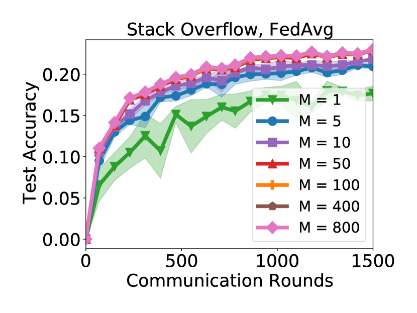
Figure 15: Average test accuracy of FedAvg versus the number of communication rounds, for various tasks and cohort sizes $M$.

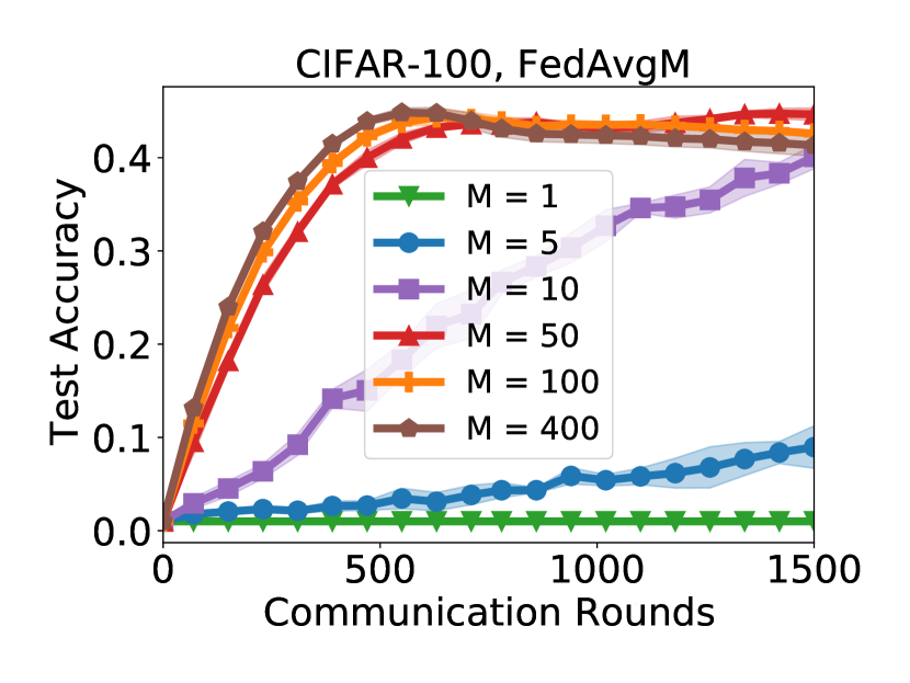
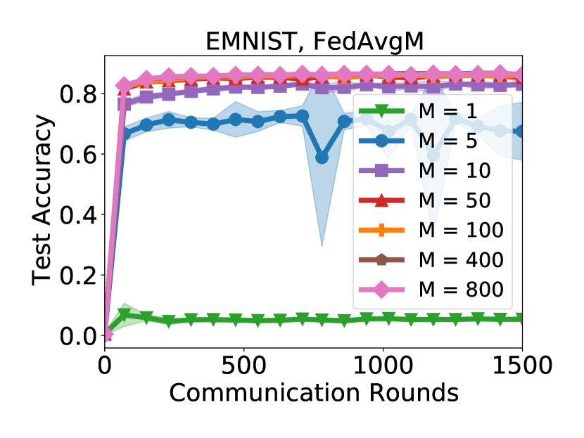
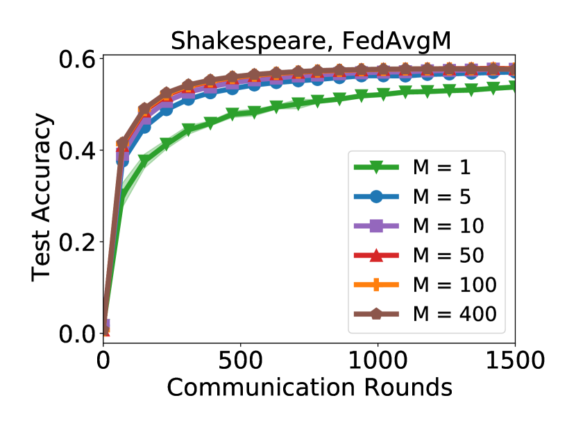
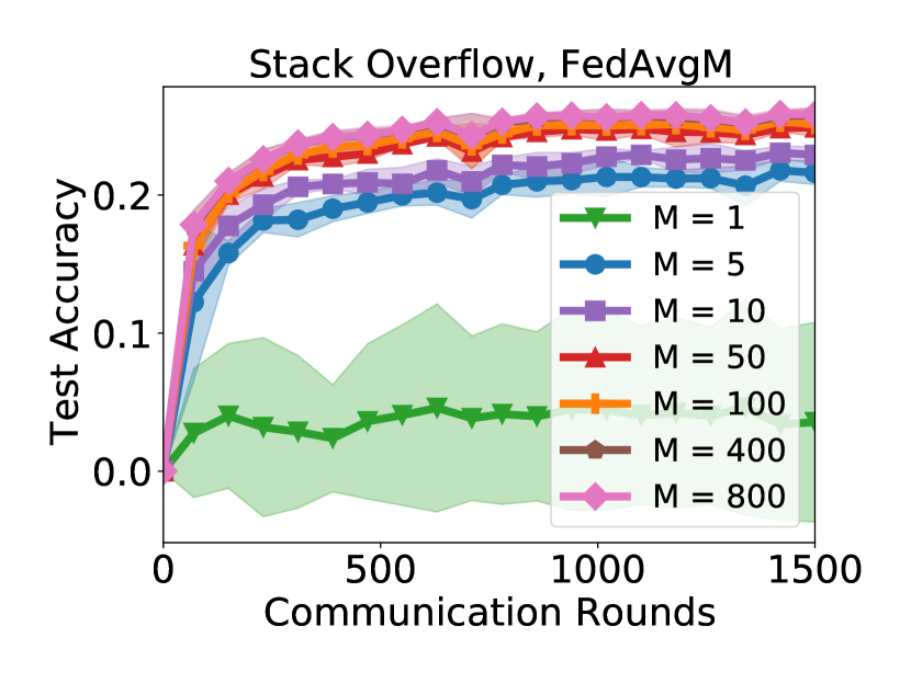
Figure 16: Average test accuracy of FedAvgM versus the number of communication rounds, for various tasks and cohort sizes $M$.

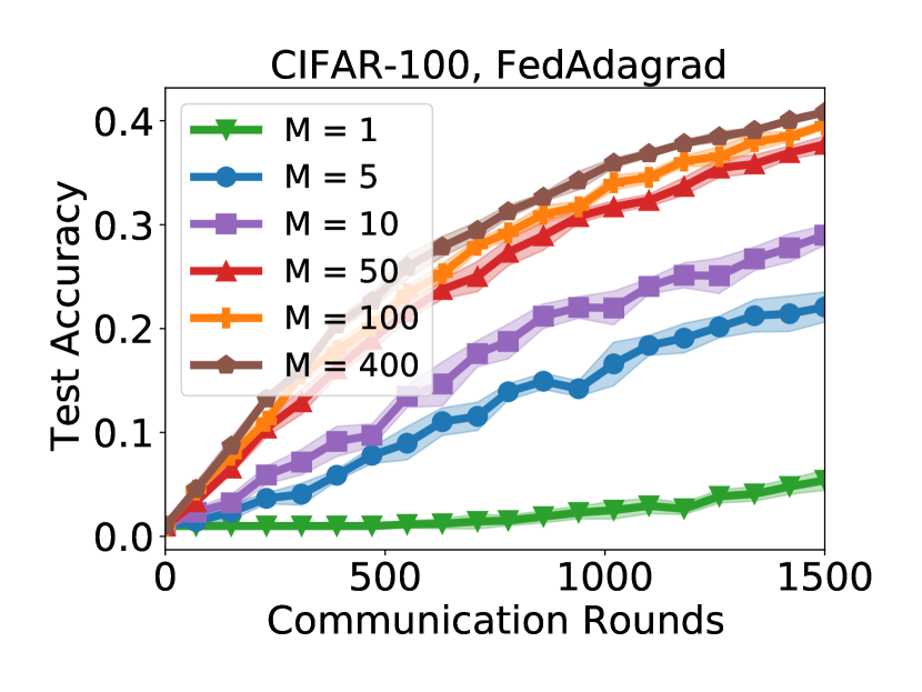
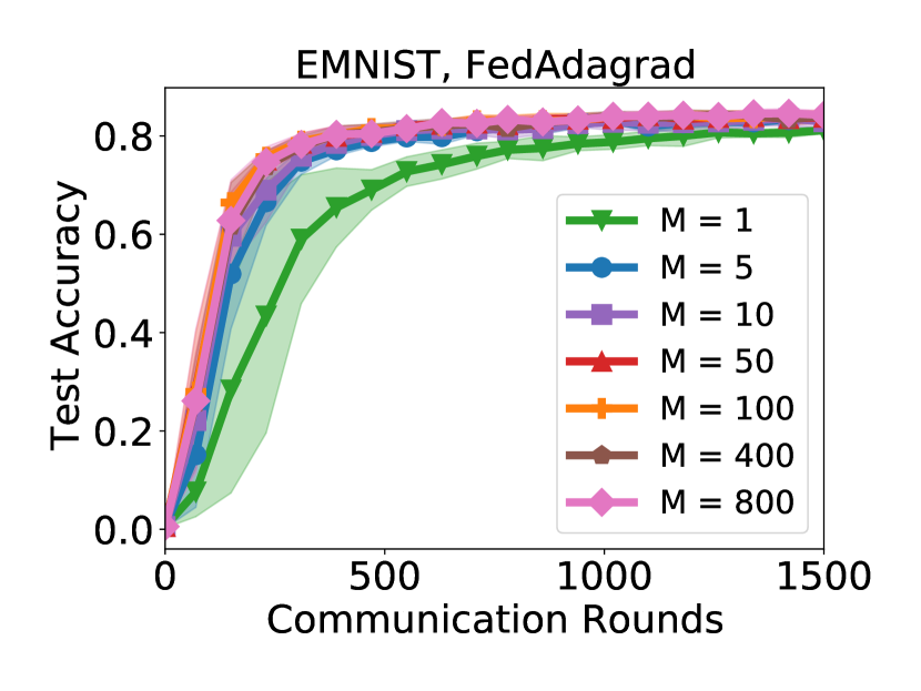
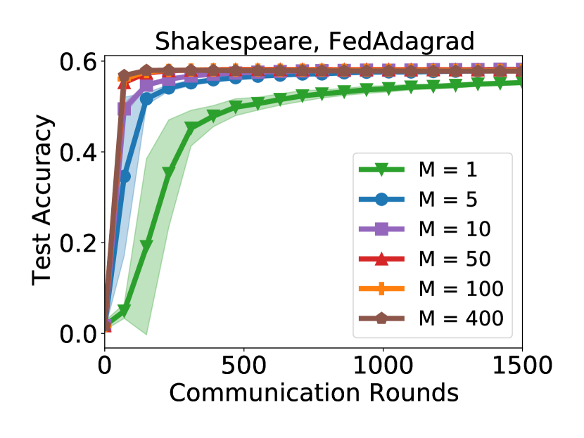
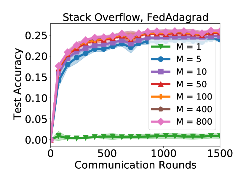
Figure 17: Average test accuracy of FedAdagrad versus the number of communication rounds, for various tasks and cohort sizes $M$.

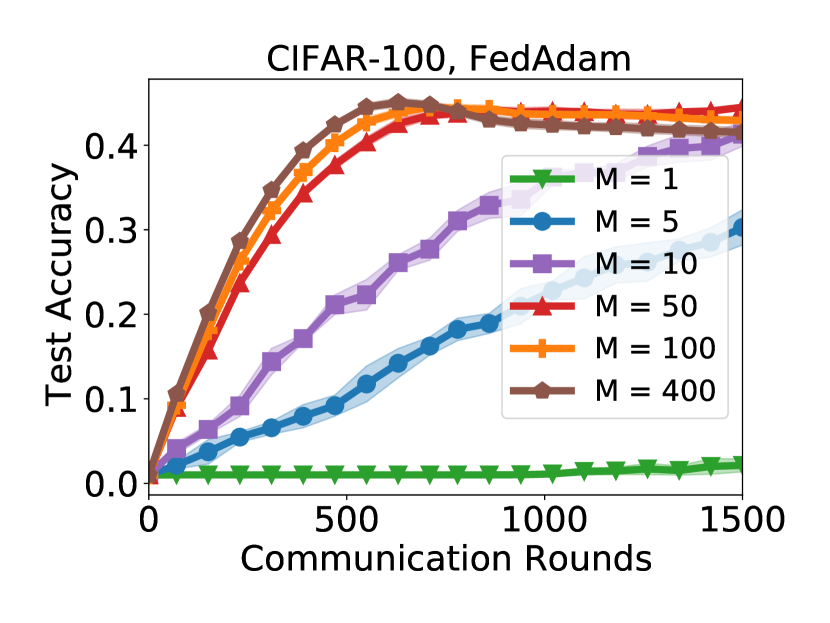
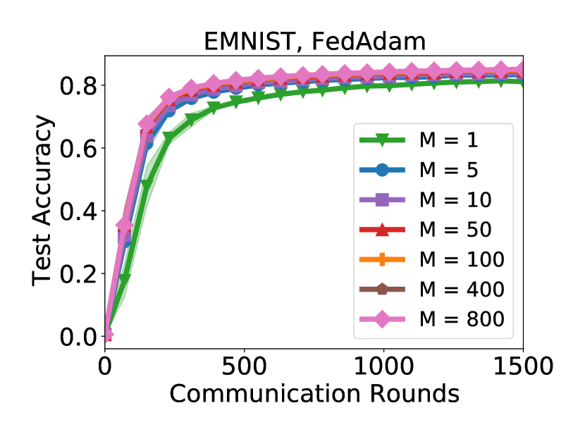
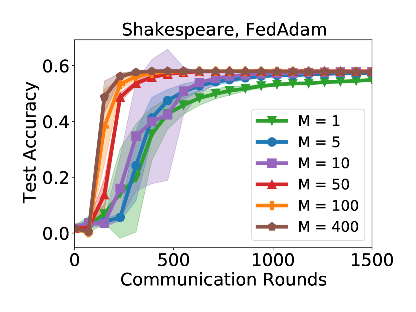
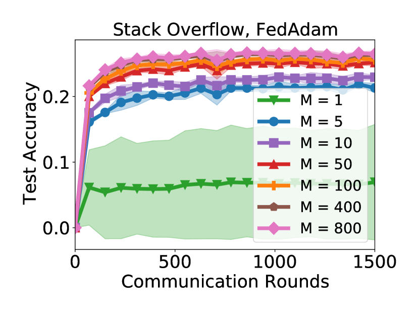
Figure 18: Average test accuracy of FedAdam versus the number of communication rounds, for various tasks and cohort sizes $M$.

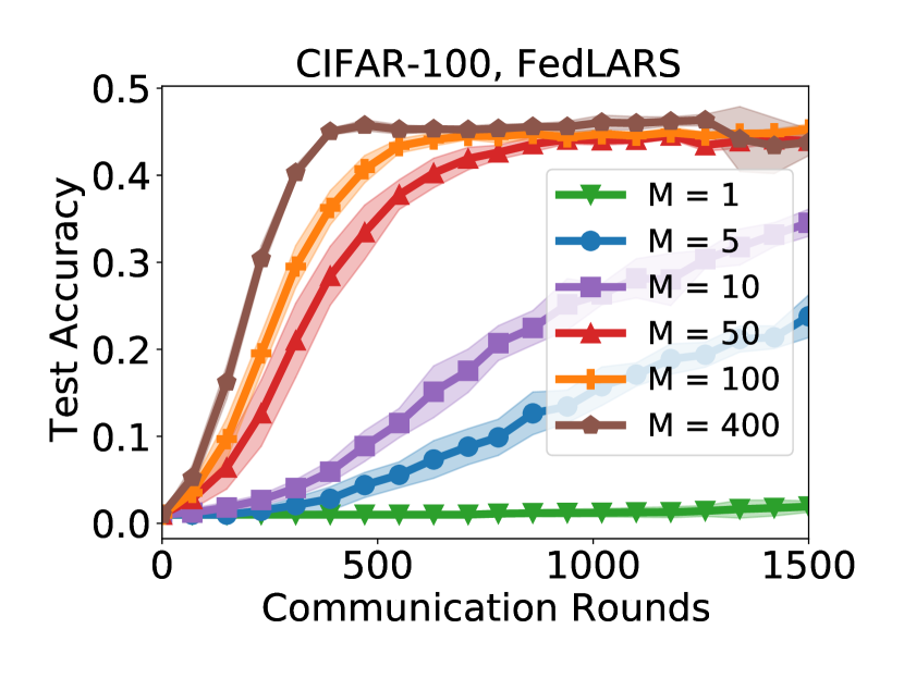
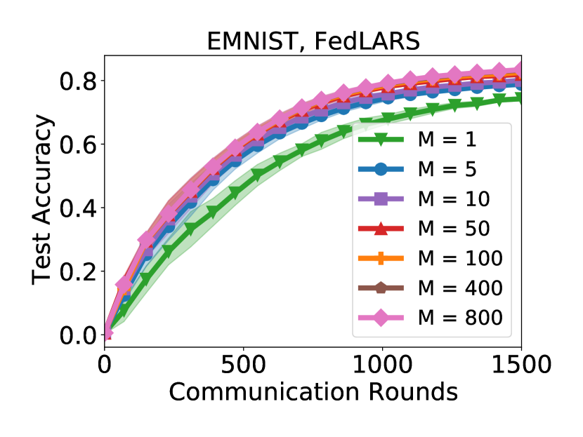
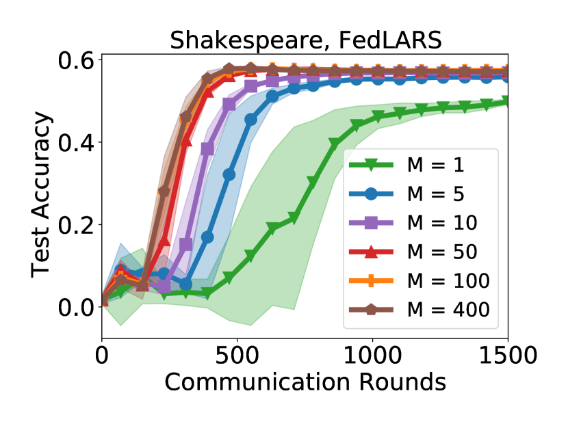
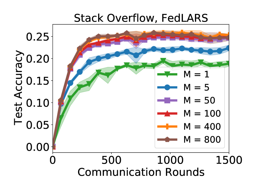
Figure 19: Average test accuracy of FedLARS versus the number of communication rounds, for various tasks and cohort sizes $M$.

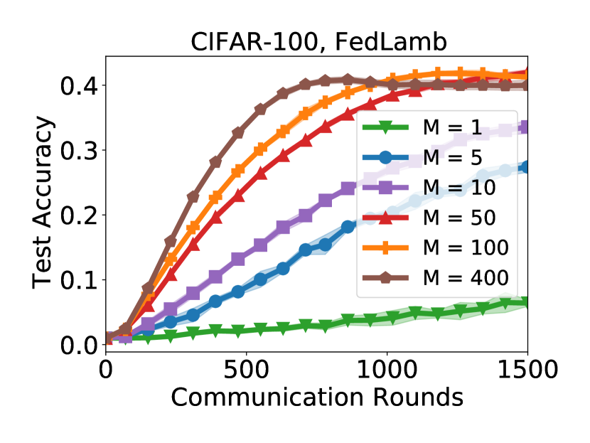
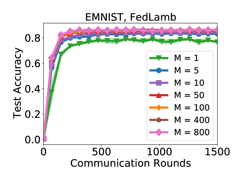
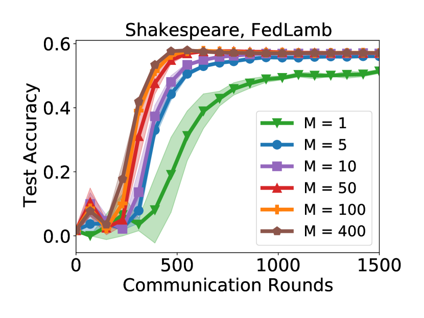
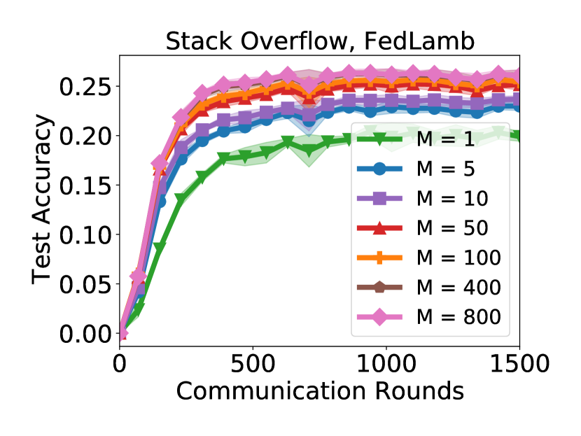
Figure 20: Average test accuracy of FedLamb versus the number of communication rounds, for various tasks and cohort sizes $M$.

B.2 Accuracy Versus Cohort Size

In this section, we showcase the train and test accuracy of various methods, as a function of the cohort size. The results are given in Figures 21 and 22, which correspond to the train and test accuracy, respectively. Both plots give the accuracy of FedAvg, FedAdam, FedAdagrad, FedLARS, and FedLamb as a function of the participation rate. That is, the percentage of training clients used in each cohort.

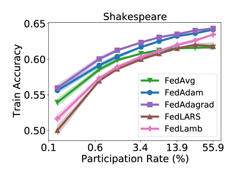
Figure 21: Train accuracy of FedAvg, FedAdam, FedAdagrad, FedLARS, and FedLamb after 1500 rounds, using varying cohort sizes and tasks. The $x$-axis denotes the percentage of training clients in each cohort.

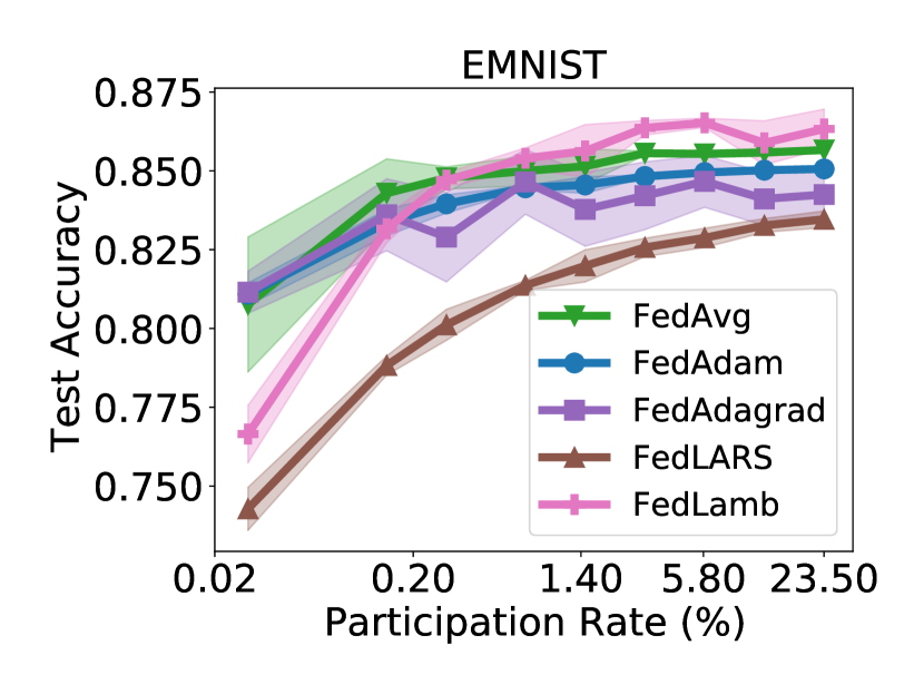
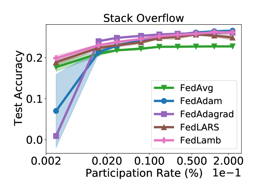
Figure 22: Test accuracy of FedAvg, FedAdam, FedAdagrad, FedLARS, and FedLamb after 1500 rounds, using varying cohort sizes and tasks. The $x$-axis denotes the percentage of training clients in each cohort.

B.3 Cohort Size Speedups

In this section, we attempt to see how much increasing the cohort size can speed up a federated algorithm. In particular, we plot the number of rounds needed to obtain a given accuracy threshold versus the cohort size. The results are given in Figures 23, 24, 25, 26, and 27. We see that in just about all cases, the speedups incurred by increasing the cohort size do not scale linearly. That being said, we still see that increasing the cohort size generally always leads to a reduction in the number of rounds needed to obtain a given test accuracy, and can lead to accuracy thresholds unobtainable by small-cohort training in communication-limited settings.

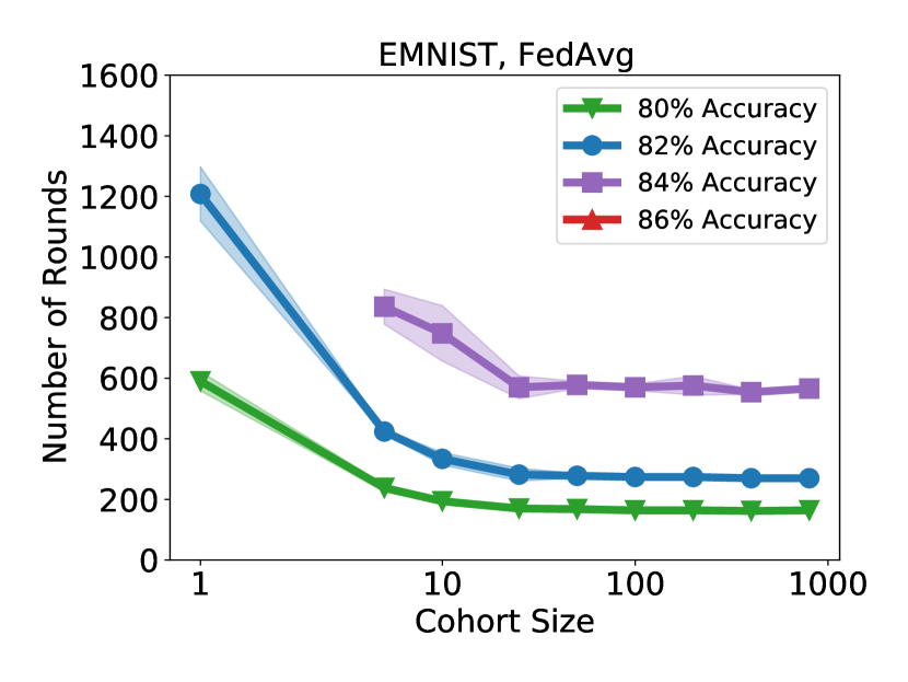
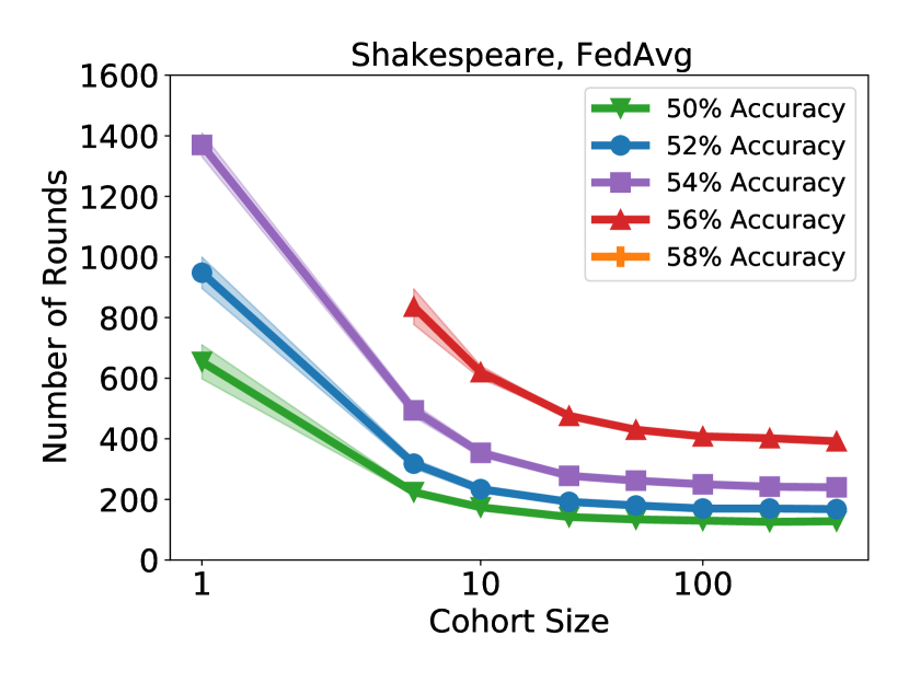
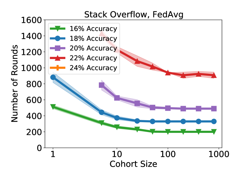
Figure 23: Number of communication rounds for FedAvg to obtain certain test accuracy thresholds. The $x$-axis denotes the cohort size.

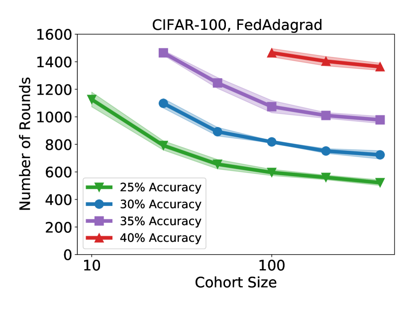
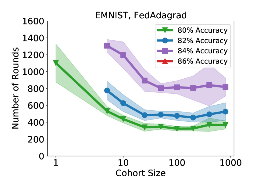
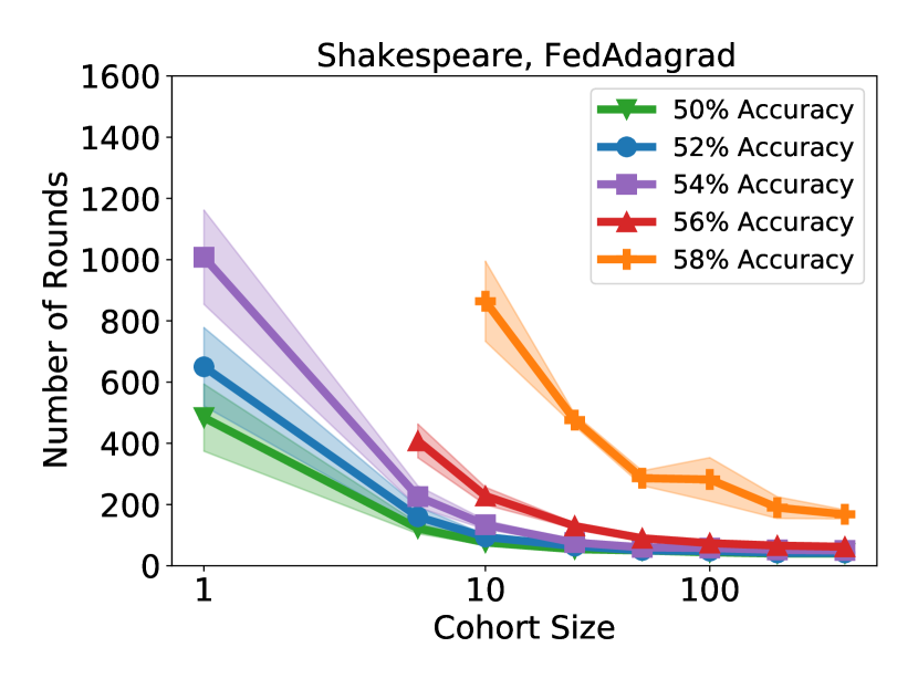
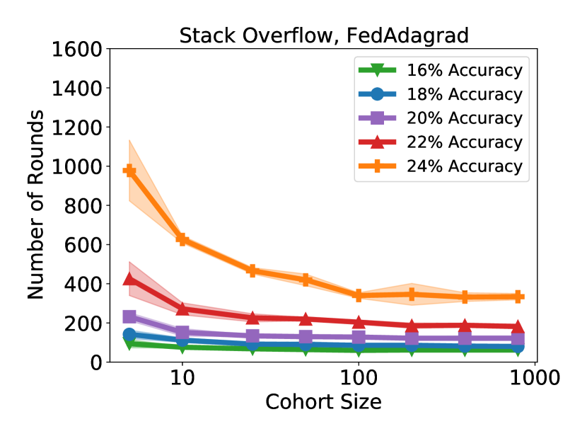
Figure 24: Number of communication rounds for FedAdagrad to obtain certain test accuracy thresholds. The $x$-axis denotes the cohort size.

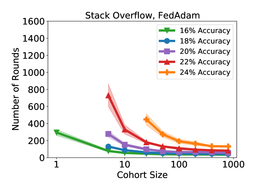
Figure 25: Number of communication rounds for FedAdam to obtain certain test accuracy thresholds. The $x$-axis denotes the cohort size.

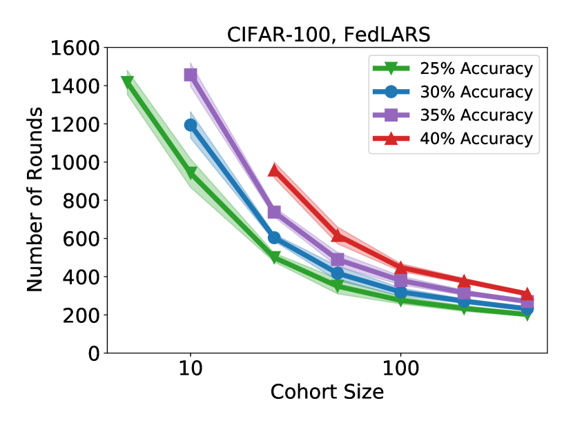
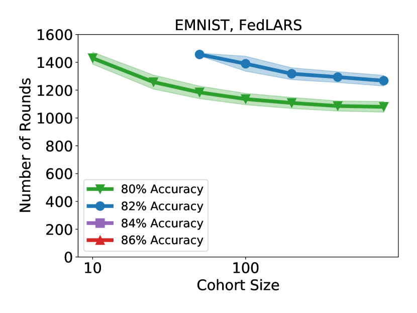
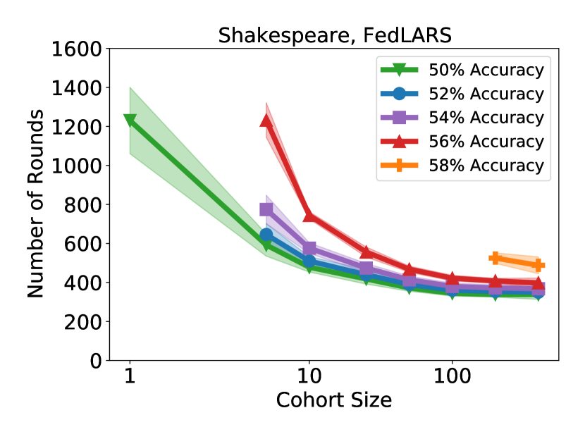
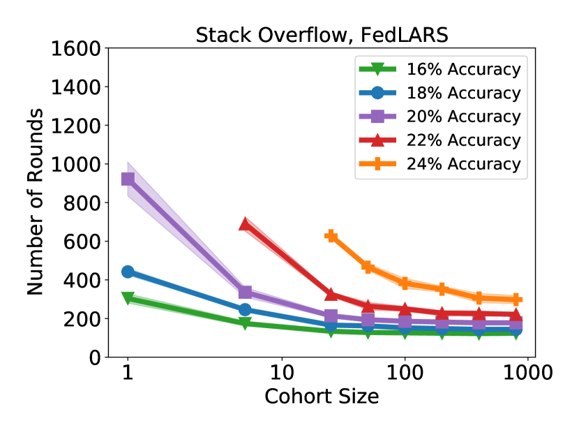
Figure 26: Number of communication rounds for FedLARS to obtain certain test accuracy thresholds. The $x$-axis denotes the cohort size.

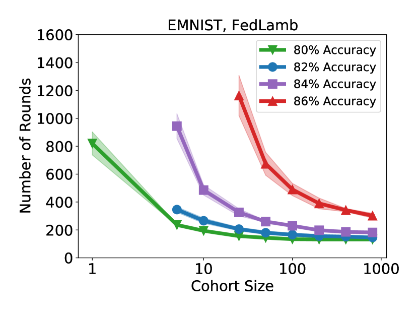
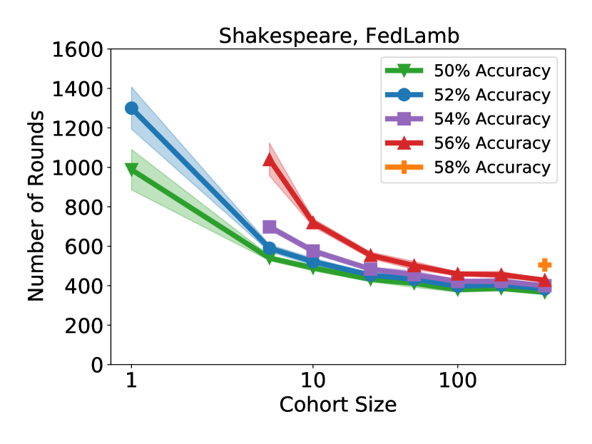
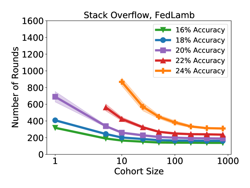
Figure 27: Number of communication rounds for FedLamb to obtain certain test accuracy thresholds. The $x$-axis denotes the cohort size.

While theory shows that in the worst-case, the cohort size leads to linear speedups, we find that this is generally not the case in practice.

B.4 Measures of Accuracy Across Clients

In this section, we expand on the fairness results in Section 3. In Tables 6, 7, 8, and 9, we present percentiles of accuracy of FedAdam across all test clients (after training for 1500 rounds, with varying cohort sizes and on varying tasks). For example, the 50th percentile of accuracy is the median accuracy of the learned model across all test clients.

The results show that in nearly all cases, the cohort size impacts all percentiles of accuracy in the same manner. For example, in Table 6, we see that a cohort size of $M=50$ is better than other cohort sizes, for all percentiles of test accuracy. Notably, this does not support the notion that larger cohorts learn more fair models. Instead, it seems that large cohorts can lead to generalization failures across all percentiles, as it does on CIFAR-100 and Shakespeare (Tables 6 and 8). However, this does not occur on EMNIST and Stack Overflow (Tables 7 and 9), which have many more train and test clients.

Table 6: Percentiles of accuracy across test clients for FedAdam on CIFAR-100 after 1500 communication rounds. We present the mean and standard deviation across 5 random trials, with the largest accuracy values for each percentile in bold.

Percentile	Cohort Size
	10	50	100	200	400
5	$27.0\pm 3.3$	$32.2\pm 1.1$	$30.6\pm 0.9$	$29.6\pm 1.1$	$29.0\pm 1.2$
25	$35.3\pm 1.5$	$39.0\pm 0.7$	$37.5\pm 0.9$	$37.2\pm 1.1$	$36.4\pm 1.1$
50	$41.1\pm 1.3$	$44.5\pm 0.5$	$43.1\pm 0.7$	$42.4\pm 0.5$	$41.6\pm 0.7$
75	$47.5\pm 1.1$	$50.1\pm 0.7$	$48.4\pm 0.5$	$47.2\pm 0.4$	$47.0\pm 1.0$
95	$54.2\pm 1.5$	$55.6\pm 1.5$	$54.6\pm 1.5$	$53.8\pm 1.3$	$53.6\pm 1.5$

Table 7: Percentiles of accuracy across test clients for FedAdam on EMNIST after 1500 communication rounds. We present the mean and standard deviation across 5 random trials, with the largest accuracy values for each percentile in bold.

Percentile	Cohort Size
	10	50	100	200	400	800
5	$61.9\pm 2.1$	$62.5\pm 2.4$	$64.3\pm 1.2$	$63.8\pm 1.4$	$64.3\pm 1.0$	$65.0\pm 0.9$
25	$77.3\pm 0.7$	$77.4\pm 1.4$	$77.9\pm 0.4$	$78.2\pm 0.4$	$78.6\pm 0.5$	$78.7\pm 0.3$
50	$84.5\pm 0.5$	$85.4\pm 0.5$	$85.9\pm 0.2$	$85.9\pm 0.2$	$86.1\pm 0.2$	$86.2\pm 0.1$
75	$91.2\pm 0.2$	$92.0\pm 0.1$	$92.0\pm 0.2$	$92.3\pm 0.1$	$92.3\pm 0.1$	$92.3\pm 0.0$
95	$100.0\pm 0.0$	$100.0\pm 0.0$	$100.0\pm 0.0$	$100.0\pm 0.0$	$100.0\pm 0.0$	$100.0\pm 0.0$

Table 8: Percentiles of accuracy across test clients for FedAdam on Shakespeare after 1500 communication rounds. We present the mean and standard deviation across 5 random trials, with the largest accuracy values for each percentile in bold.

Percentile	Cohort Size
	10	50	100	200	400
5	$39.9\pm 0.8$	$39.2\pm 1.8$	$39.4\pm 1.6$	$37.8\pm 0.7$	$38.6\pm 1.2$
25	$54.9\pm 0.1$	$55.0\pm 0.2$	$54.9\pm 0.2$	$54.9\pm 0.1$	$54.9\pm 0.2$
50	$58.3\pm 0.2$	$58.5\pm 0.2$	$58.5\pm 0.2$	$58.3\pm 0.1$	$58.4\pm 0.1$
75	$61.8\pm 0.2$	$62.4\pm 0.2$	$62.2\pm 0.2$	$62.1\pm 0.2$	$62.1\pm 0.3$
95	$70.9\pm 0.6$	$71.2\pm 0.6$	$71.2\pm 0.4$	$71.1\pm 0.2$	$71.1\pm 0.2$

Table 9: Percentiles of accuracy across test clients for FedAdam on Stack Overflow after 1500 communication rounds. We present the mean and standard deviation across 5 random trials, with the largest accuracy values for each percentile in bold.

Percentile	Cohort Size
	10	50	100	200	400	800
5	$16.7\pm 0.2$	$18.7\pm 0.2$	$19.1\pm 0.2$	$19.5\pm 0.1$	$19.8\pm 0.1$	$19.9\pm 0.1$
25	$21.0\pm 0.3$	$23.2\pm 0.2$	$23.6\pm 0.2$	$24.1\pm 0.1$	$24.4\pm 0.1$	$24.5\pm 0.1$
50	$23.5\pm 0.3$	$25.8\pm 0.2$	$26.3\pm 0.3$	$26.7\pm 0.1$	$27.0\pm 0.1$	$27.2\pm 0.1$
75	$26.1\pm 0.3$	$28.4\pm 0.2$	$29.0\pm 0.3$	$29.4\pm 0.1$	$29.7\pm 0.1$	$29.9\pm 0.1$
95	$30.8\pm 0.3$	$33.2\pm 0.2$	$33.7\pm 0.4$	$34.2\pm 0.1$	$34.6\pm 0.1$	$34.8\pm 0.1$

B.5 Simulating Straggler Effects

As shown in Section 3.5, large-cohort training methods seem to face data-efficiency issues, where training with large cohorts requires processing many more examples to reach accuracy thresholds than small-cohort training. While this is related to diminishing returns (Section 3.2) and occurs in large-batch training as well (Golmant et al., 2018), we highlight this issue due to its consequences in federated learning.

Unlike centralized learning, federated learning faces fundamental limits on parallelization. Since data cannot be shared, we typically cannot scale up to arbitrarily large cohort sizes. Instead, the parallelization is limited by the available training clients. In order to learn on a client’s local dataset, that client must actually perform the training on its examples. Unfortunately, since clients are often lightweight in cross-device settings (Kairouz et al., 2021), clients with many examples may require longer compute times, becoming stragglers in a given communication round. If an algorithm is data-inefficient, these straggler clients may have to participate many times throughout training, causing the overall runtime to be greater. In short, data inefficiency can dramatically slow down large-cohort training algorithms.

To exemplify this, we compute simulated runtimes of federated algorithms under a version of the probabilistic straggler model from (Lee et al., 2017). We model each client’s runtime as a random variable drawn from a shifted exponential distribution. Such models were found to be good models of runtimes for file queries in cloud storage systems (Liang and Kozat, 2014) and mini-batch SGD on distributed compute systems (Lee et al., 2017).

In our model, we assume that the time a client requires to perform local training is some constant proportional to the number of examples the client has, plus an exponential random variable. More formally, let $N_{k}$ denote the number of examples held by some client $k$, and let $X_{k}$ denote the amount of time required by client $k$ to perform their local training in Algorithm 1. Then we assume that there are constants $\alpha,\lambda>0$ such that

$$X_{k}-\alpha N_{k}\sim\text{Exp}\left(\frac{1}{\lambda N_{k}}\right).$$

Here $\lambda$ is the straggler parameter. Recall that if $X\sim\text{Exp}(1/\lambda)$, then $\mathbb{E}[X]=\lambda$. Therefore, we assume that the expected runtime of client $k$ equal $\alpha N$ plus some random variable whose expected value is $\lambda N$. Thus, larger $\lambda$ means larger expected client runtimes. By convention, we can also use $\lambda=0$ in which case $X_{k}=\alpha N_{k}$. For a given round $t$ of Algorithm 1, let $C_{t}$ denote the cohort sampled. Since Algorithm 1 requires all clients to finish before updating its global model, we model the runtime $Y_{t}$ of round $t$ as

$$Y_{t}=\max_{k\in C_{t}}\left\{X_{k}\right\}.$$

Thus, the round runtime is the maximum of $M$ shifted exponential random variables, where $M$ is the cohort size. Note that this only models the client computation time, not the server computation time or communication time. Using this model, we plot the simulated runtime of FedAvg on various tasks, for varying cohort sizes. For simplicity, we assume $\alpha=1$ in all experiments, and vary $\lambda$ over $\{0.1,1,10,100\}$. To showcase how much longer the runtime of large-cohort training may be, we present the simulated runtime, relative to $M=10$. For $a\in[0,1]$, we plot the ratio of how long it takes to reach a test accuracy of $a$ with a cohort size of $M$, versus how long it takes to reach $a$ with $M=10$. We give the results for CIFAR-100, EMNIST, Shakespeare, and Stack Overflow in Figures 28, 29, 30, 31, respectively.

When $\lambda$ is small, we see that larger cohorts can obtain higher test accuracy in a comparable amount of time to $M=10$. However, when $\lambda$ is large, large-cohort training may require anywhere from 5-10 times more client compute time. This is particularly important in cross-device settings with lightweight edge devices, as the straggler effect (which essentially increases with $\lambda$) may be larger. Note that we see particularly large increases in relative runtimes for smaller accuracy thresholds, which suggests that the dynamic cohort strategy from Section 5 may be useful in helping mitigate such issues.

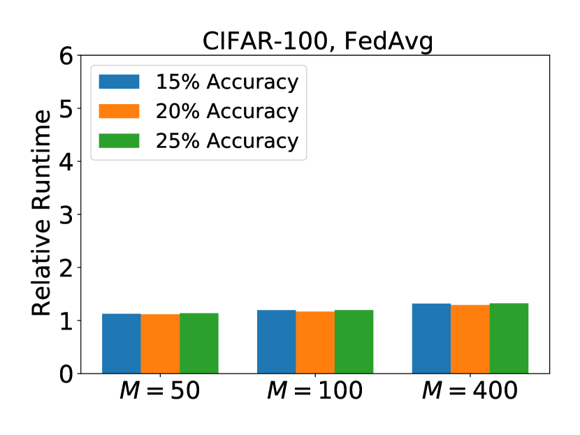
(a) $\lambda=0.1$

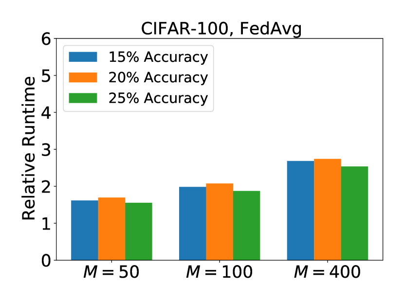
(b) $\lambda=1$

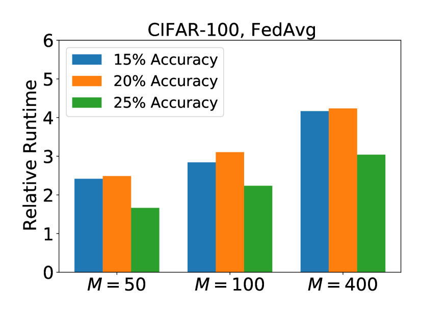
(c) $\lambda=10$

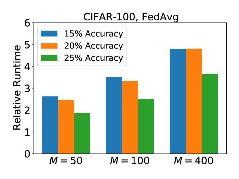
(d) $\lambda=100$

Figure 28: The relative amount of time required to reach given test accuracies on CIFAR-100 with varying cohort sizes. We present the ratio of the runtime needed for $M>10$ with respect to the time needed for $M=10$. Runtimes are simulated under a shifted exponential model with $\alpha=1$ and varying $\lambda$.

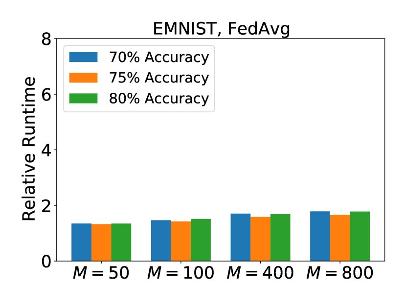
(a) $\lambda=0.1$

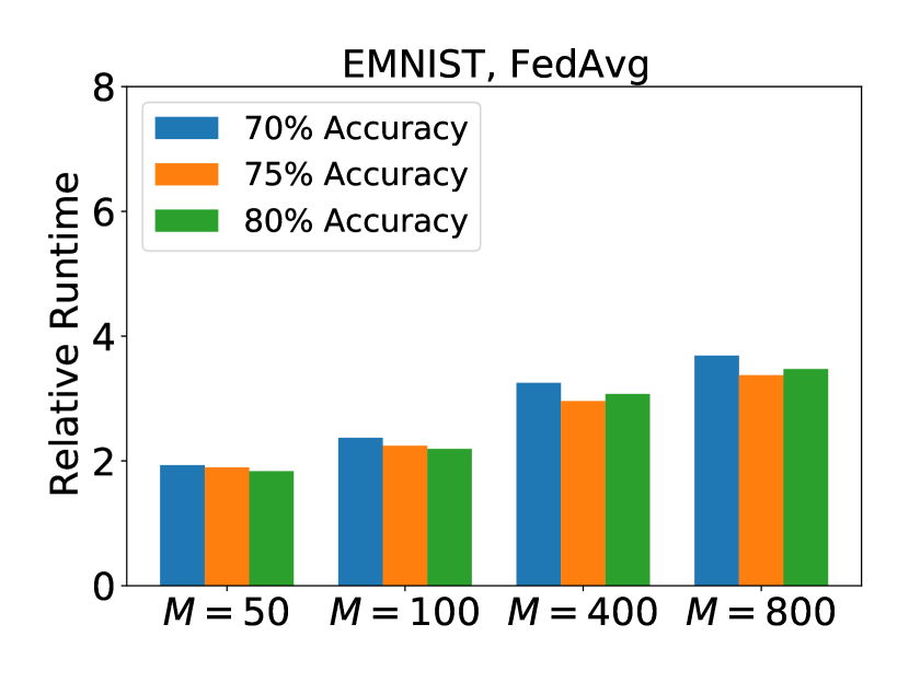
(b) $\lambda=1$

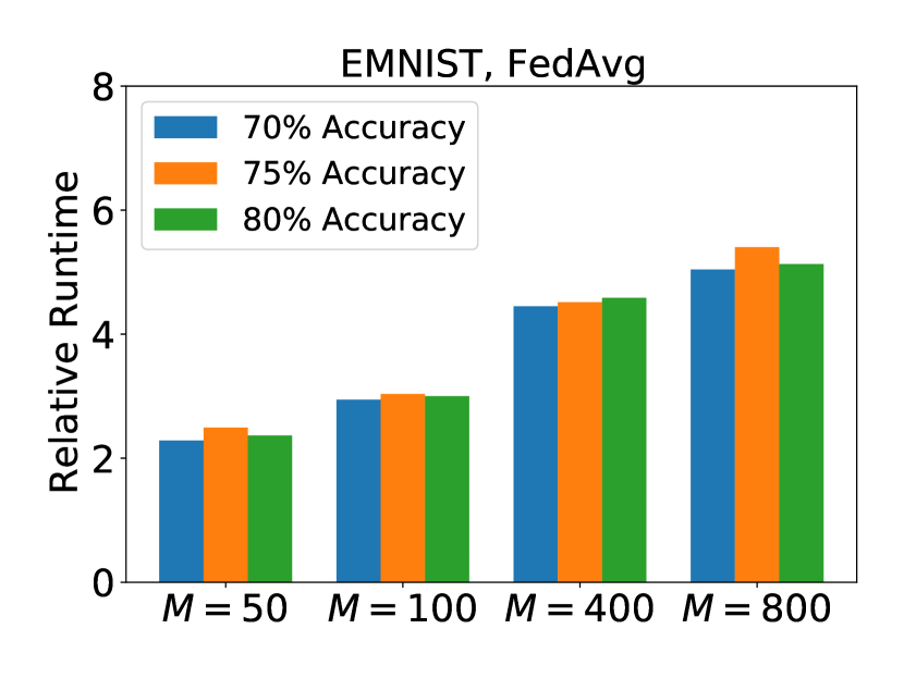
(c) $\lambda=10$

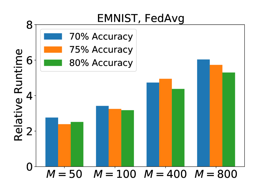
(d) $\lambda=100$

Figure 29: The relative amount of time required to reach given test accuracies on EMNIST with varying cohort sizes. We present the ratio of the runtime needed for $M>10$ with respect to the time needed for $M=10$. Runtimes are simulated under a shifted exponential model with $\alpha=1$ and varying $\lambda$.

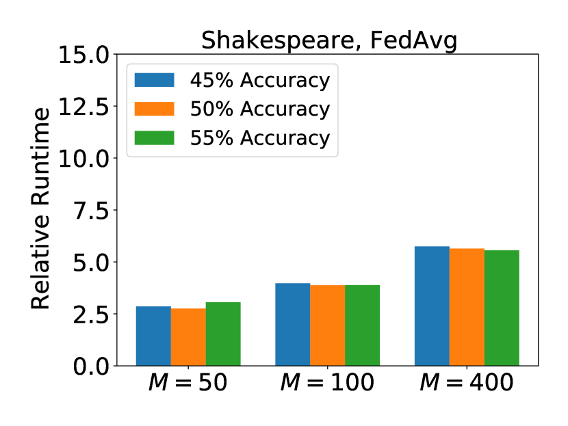
(a) $\lambda=0.1$

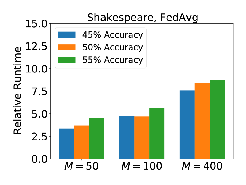
(b) $\lambda=1$

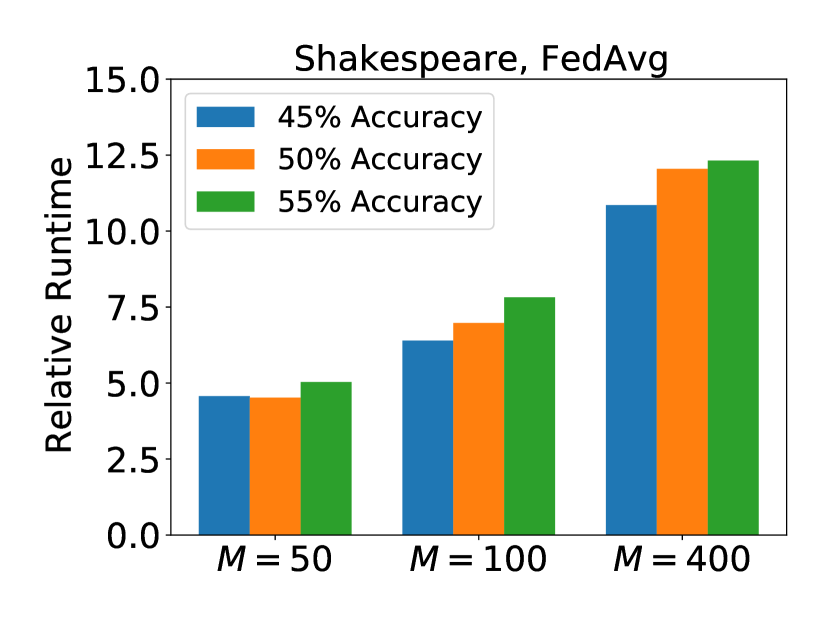
(c) $\lambda=10$

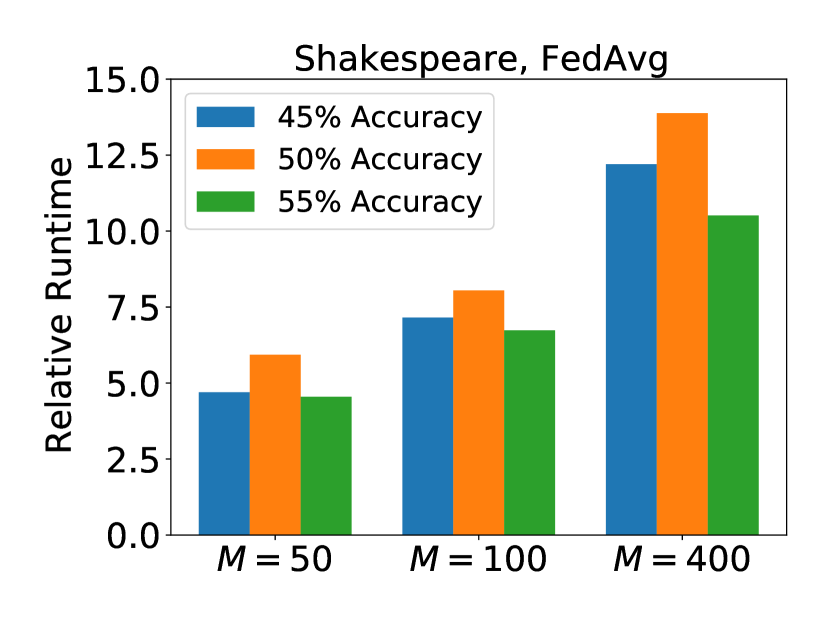
(d) $\lambda=100$

Figure 30: The relative amount of time required to reach given test accuracies on Shakespeare with varying cohort sizes. We present the ratio of the runtime needed for $M>10$ with respect to the time needed for $M=10$. Runtimes are simulated under a shifted exponential model with $\alpha=1$ and varying $\lambda$.

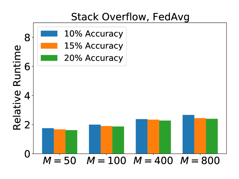
(a) $\lambda=0.1$

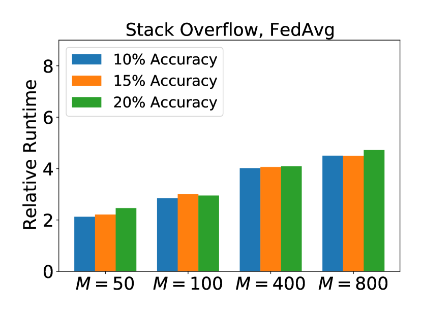
(b) $\lambda=1$

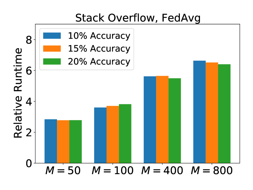
(c) $\lambda=10$

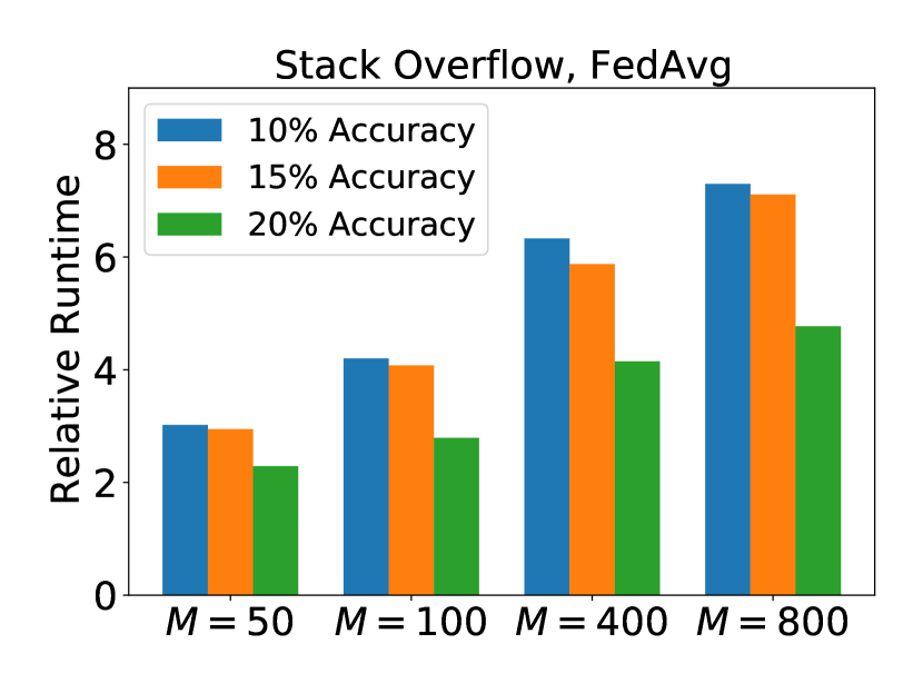
(d) $\lambda=100$

Figure 31: The relative amount of time required to reach given test accuracies on Stack Overflow with varying cohort sizes. We present the ratio of the runtime needed for $M>10$ with respect to the time needed for $M=10$. Runtimes are simulated under a shifted exponential model with $\alpha=1$ and varying $\lambda$.

B.6 Pseudo-Gradient Norms

In this section, we present the norm of the server pseudo-gradient $\Delta$ in Algorithm 1 with respect to the number of communication rounds. We do this for varying cohort sizes and tasks across 1500 communication rounds. All plots give the $\ell_{2}$ norm of $\Delta$. The results are given in Figures 32, 33, 34, 35, 36, 37, and 38. These gives the results for FedSGD, FedAvg, FedAvgM, FedAdagrad, FedAdam, FedLARS, and FedLamb (respectively).

We find that in nearly all cases, the results for FedSGD differ from all other algorithms. While there is significant overlap in the pseudo-gradient norm for FedSGD across all cohort sizes (Figure 32), any method that uses multiple local training steps generally does not see such behavior. The only notable counter-example is FedAdagrad on EMNIST (Figure 35). Otherwise, both non-adaptive and adaptive federated methods that use local training (such as FedAvg, FedAdam, and FedLamb) see similar behavior: The pseudo-gradient norm is effectively stratified by the cohort size. Larger cohort sizes lead to smaller pseudo-gradient norms, with little overlap. Moreover, as discussed in Section 4, we see that after enough communication rounds occur, the pseudo-gradient norm obeys an inverse square root scaling rule.

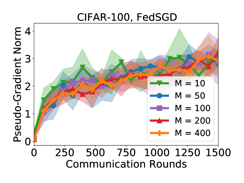
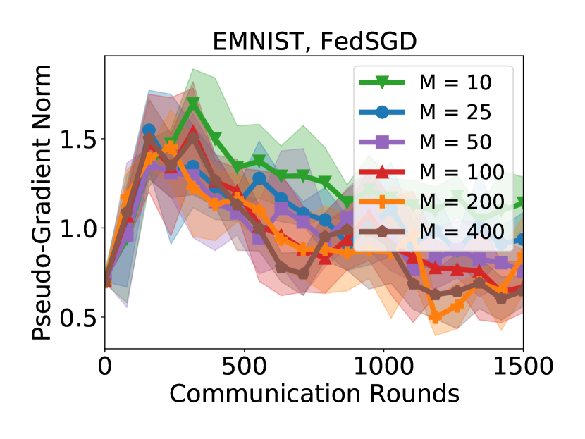
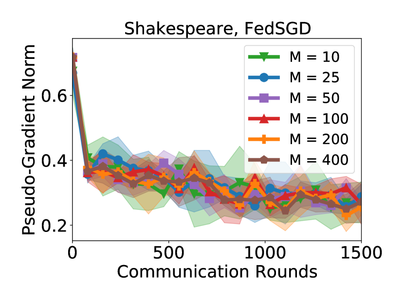
Figure 32: Average pseudo-gradient norm of FedSGD versus the number of communication rounds, for various tasks and cohort sizes $M$.

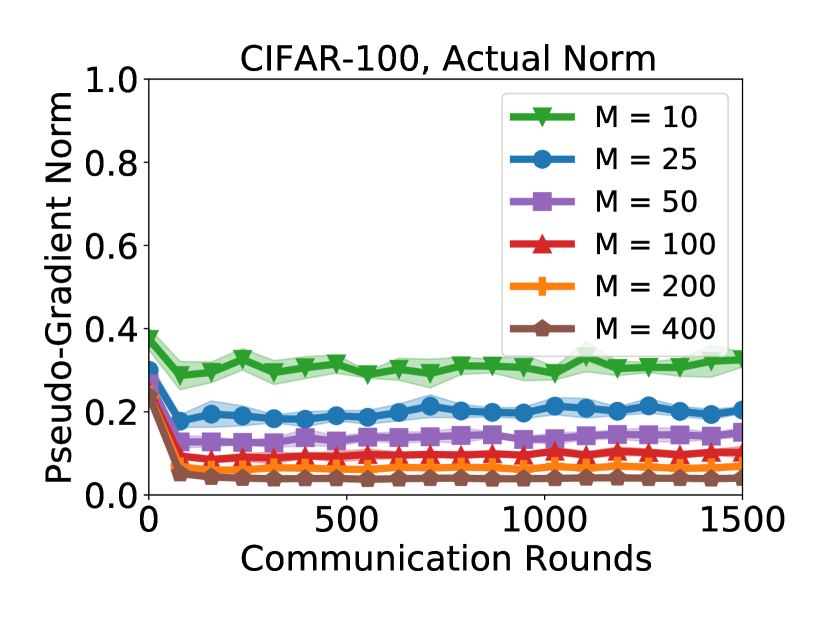
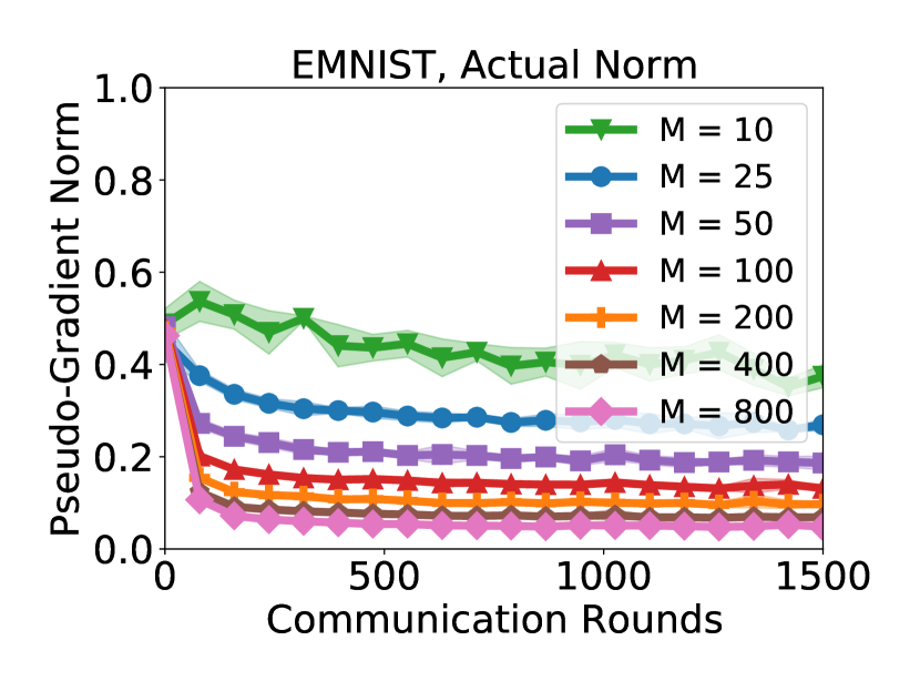
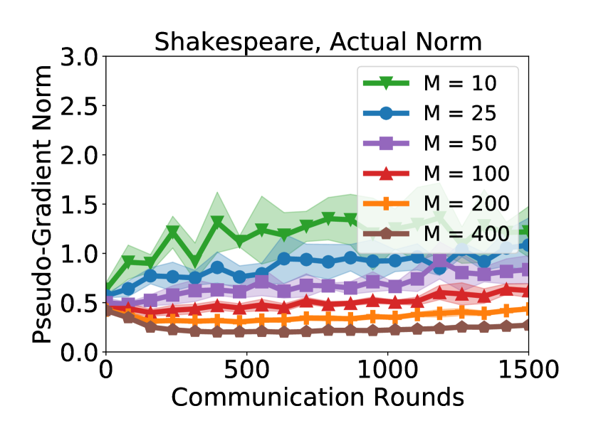
Figure 33: Average pseudo-gradient norm of FedAvg versus the number of communication rounds, for various tasks and cohort sizes $M$.

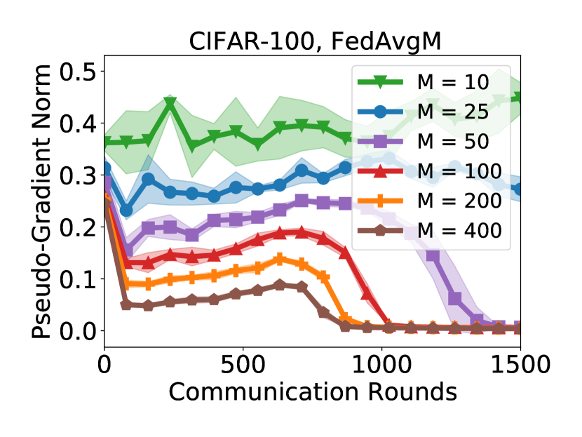
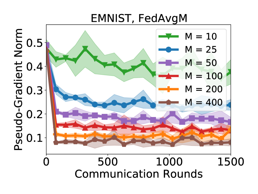
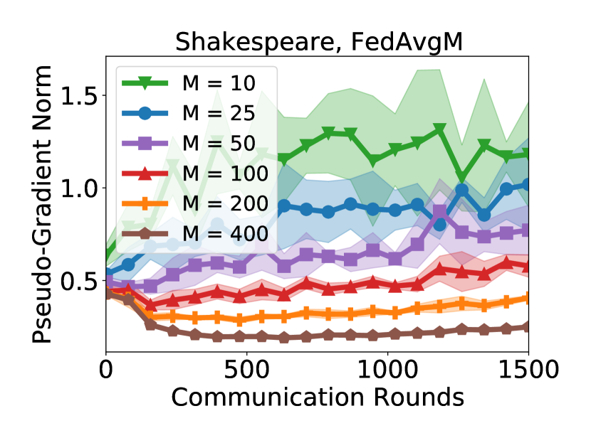
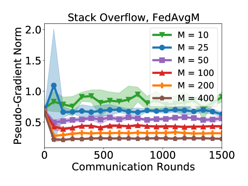
Figure 34: Average pseudo-gradient norm of FedAvgM versus the number of communication rounds, for various tasks and cohort sizes $M$.

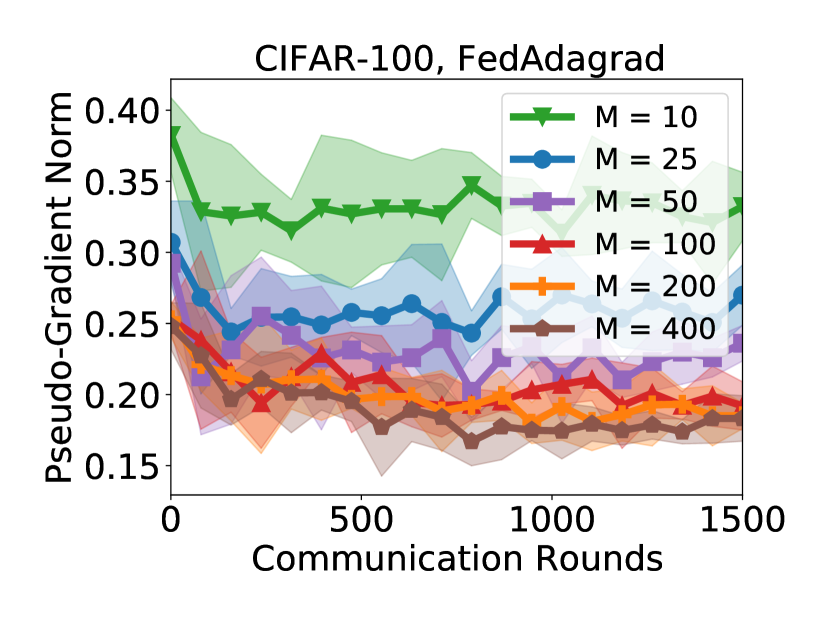
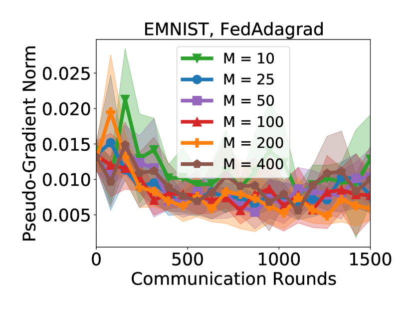
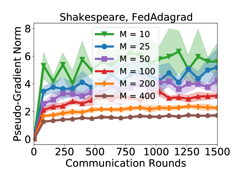
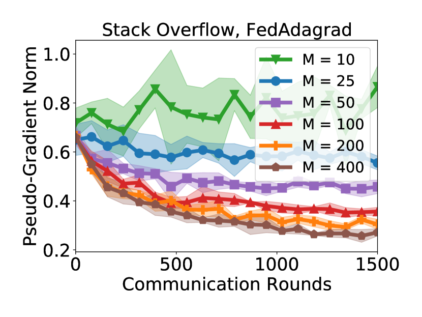
Figure 35: Average pseudo-gradient norm of FedAdagrad versus the number of communication rounds, for various tasks and cohort sizes $M$.

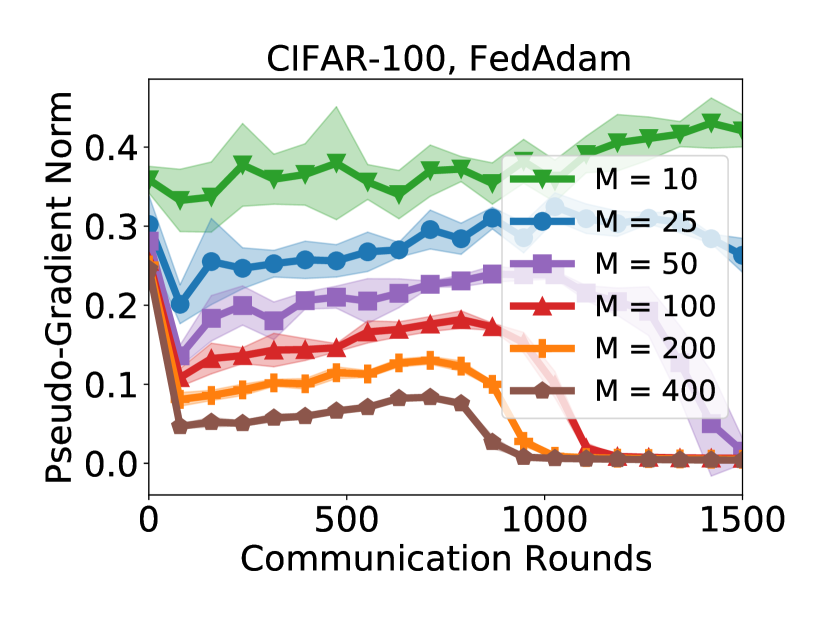
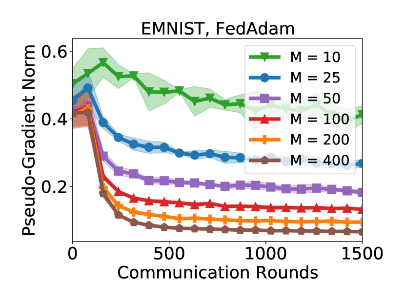
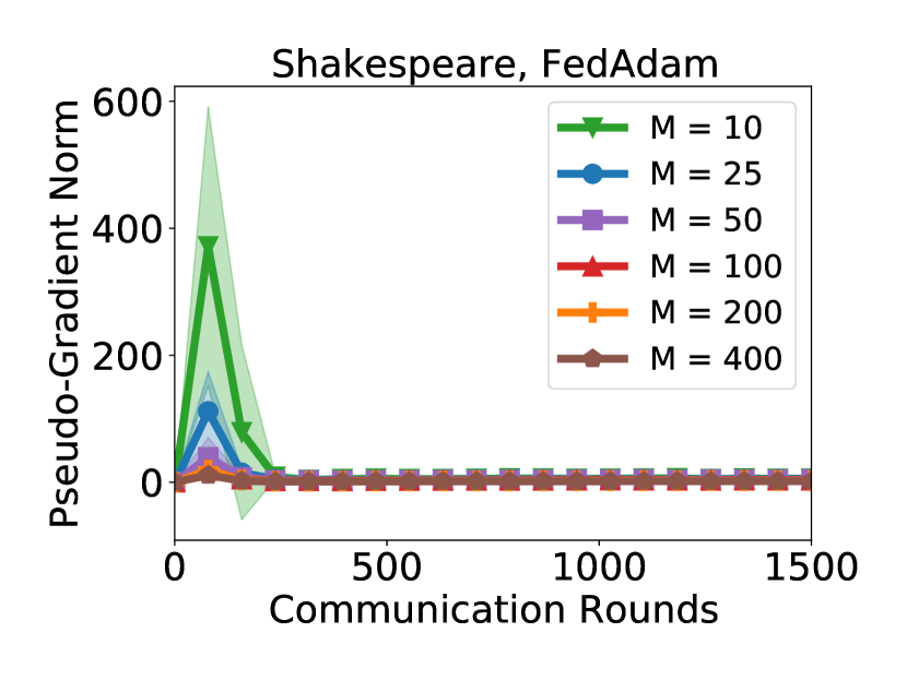
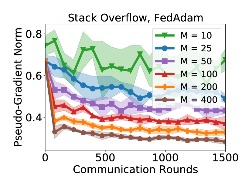
Figure 36: Average pseudo-gradient norm of FedAdam versus the number of communication rounds, for various tasks and cohort sizes $M$.

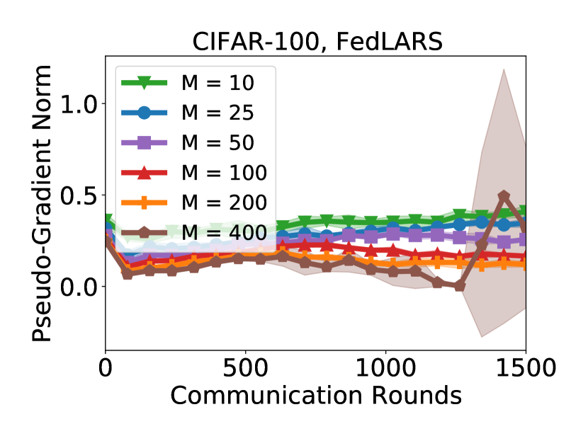
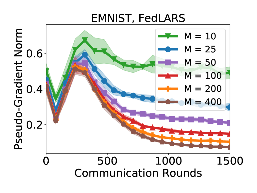
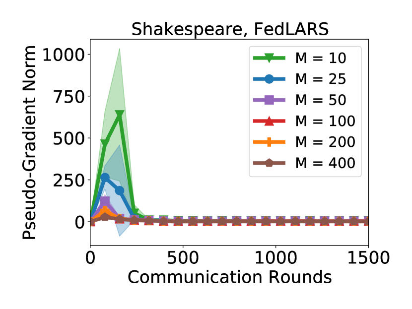
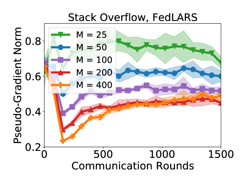
Figure 37: Average pseudo-gradient norm of FedLARS versus the number of communication rounds, for various tasks and cohort sizes $M$.

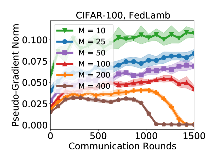
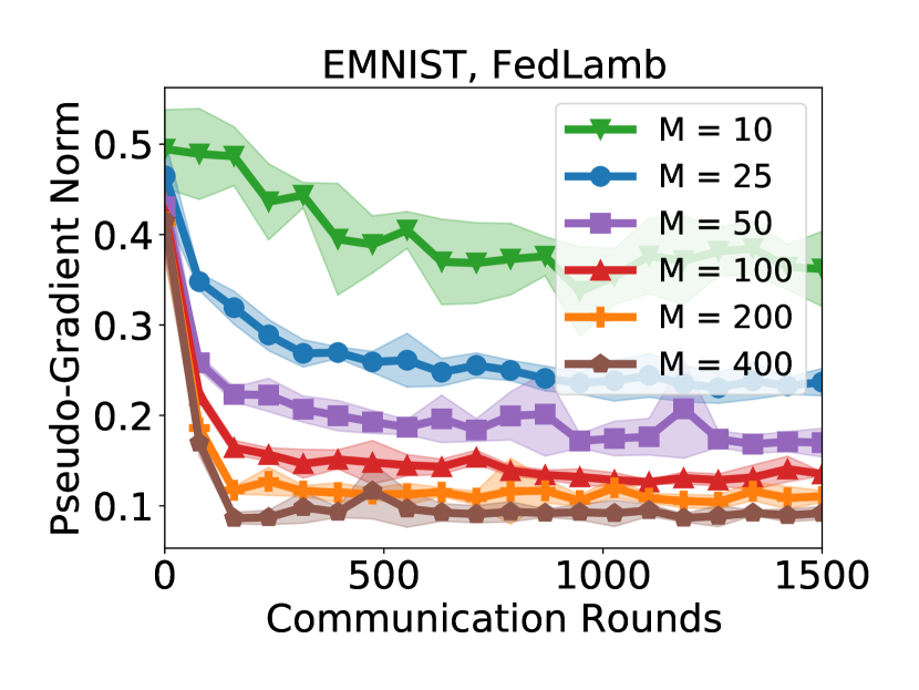
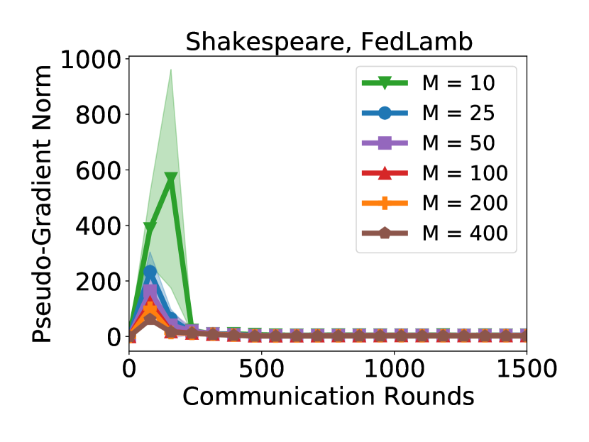
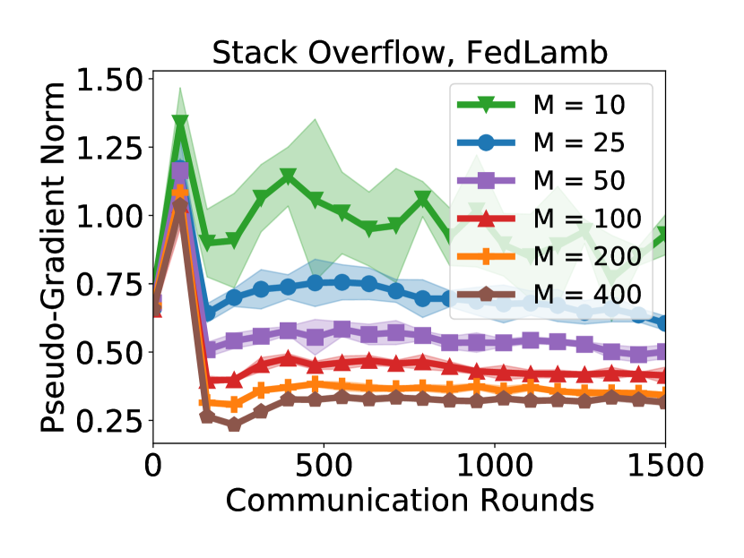
Figure 38: Average pseudo-gradient norm of FedLamb versus the number of communication rounds, for various tasks and cohort sizes $M$.

B.6.1 Cosine Similarity of Client Updates

Recall that in Section 4, we showed that for FedAvg, client updates are nearly orthogonal on the Stack Overflow task. In this section, we show that this holds across tasks. In Figure 39, we present the average cosine similarity between distinct clients in each training round, for FedAvg and FedSGD. Thus, given a cohort size $M$, at each round $t$ we compute $\binom{|M|}{2}$ cosine similarities between client updates, and take the average over all pairs. Formally, we compute, for each round $t$,

$$\theta_{t}:=\binom{|C_{t}|}{2}^{-1}\sum_{\begin{subarray}{c}i,j\in C_{t}\\ i\neq j\end{subarray}}\dfrac{\left\langle\Delta_{i}^{t},\Delta_{j}^{t}\right\rangle}{\|\Delta_{i}^{t}\|_{2}\|\Delta_{j}^{t}\|_{2}}$$ (5)

where $C_{t}$ is the cohort of sampled clients in round $t$, and $\Delta_{k}^{t}$ denotes the client update of client $k\in C_{t}$ (see Algorithm 1). Note that because we normalize, it does not matter whether we use clipping or not (Algorithm 2). The results for $\theta_{t}$ with cohort size $M=50$ are given in Figure 39.

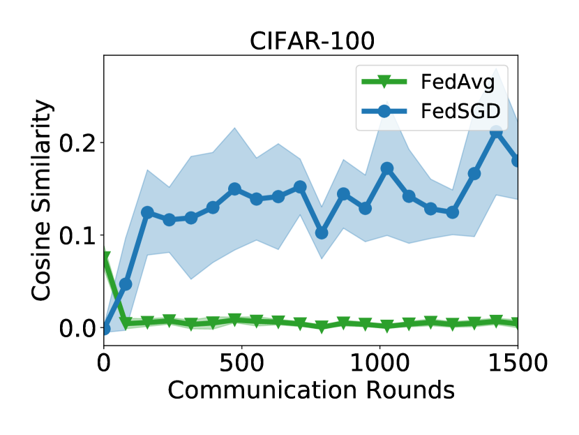
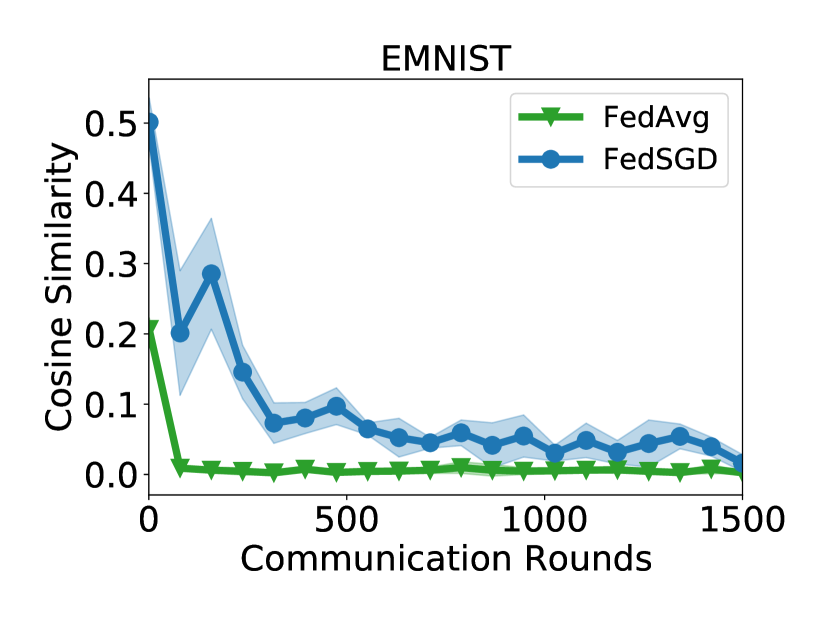
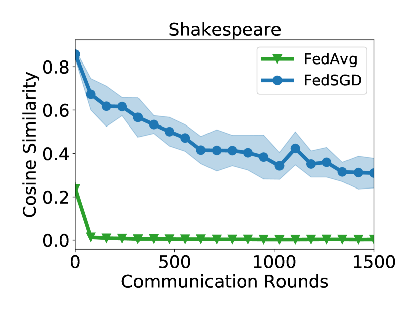
Figure 39: Average cosine similarity $\theta_{t}$ (as in (5)) between client updates $\Delta_{k}^{t}$ with respect to the number of communication rounds, for FedAvg on EMNIST with a cohort size of $M=50$.

We see that in all cases, after a small number of communication rounds, $\theta_{t}$ becomes close to zero for FedAvg. By contrast, $\theta_{t}$ is not nearly as small for FedSGD, especially in intermediate rounds. We note that for EMNIST, the cosine similarity for FedSGD approaches that of FedAvg as $T\to 1500$.

B.7 Server Learning Rate Scaling

In this section, we present our full results using the learning rate scaling methods proposed in Section 5. Recall that our methods increase the server learning rate $\eta_{s}$ in accordance with the cohort size. To do so, we fix a learning rate $\eta_{s}$ for some cohort size $M$. As in (3), for $M^{\prime}\geq M$, we use a server learning rate $\eta_{s}^{\prime}$

$$\eta_{s}^{\prime}=r\left(\frac{M^{\prime}}{M}\right)\eta_{s}$$

where $r:\mathbb{R}_{\geq 0}\to\mathbb{R}_{\geq 0}$ determines the scaling rate. In particular, we focus on $r(a)=\sqrt{a}$ (square root scaling) and $r(a)=a$ (linear scaling). These rules both can be viewed as federated analogs of learning rate scaling techniques used for large-batch training (Krizhevsky, 2014; Goyal et al., 2017). We use them with a federated version of the warmup technique proposed by Goyal et al. (2017), where we linearly increase the server learning rate from $0$ to $\eta_{s}^{\prime}$ over the first $W=100$ communication rounds.

Despite the historical precedent for the linear scaling rule (Goyal et al., 2017), we find that it leads to catastrophic training failures in the federated regime, even with adaptive clipping. To showcase this, we plot the accuracy of FedAvg on EMNIST with the linear scaling rule in Figure 40. We plot the test accuracy over time, averaged across 5 random trials, for various cohort sizes $M$. While $M=50,100$ see similar convergence as in Figure 15, for $M=200$, we saw one catastrophic training failure across all 5 trials. Using $M\geq 400$, we found that all trials resulted in catastrophic training failures. In short, linear scaling can be too aggressive in federated settings, potentially due to heterogeneity among clients (which intuitively requires some amount of conservatism in server model updates).

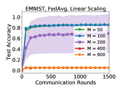
Figure 40: The test accuracy of FedAvg on EMNIST with the linear scaling rule, across 5 random trials. The mean accuracy is given in bold, with the standard deviation indicated by the pale region. We see that for $M=200$, there are a number of catastrophic training failures, while for $M\geq 400$, all trials experienced catastrophic training failures.

By contrast, the square root scaling rule did not lead to such training failures. We plot the training accuracy and test accuracy of FedAvg using the square root scaling rule in Figure 41. We plot this with respect to the cohort size, with and without the scaling rule. We see that the performance of the scaling rule is decidedly mixed. While it leads to significant improvements in training accuracy for CIFAR-100 and Shakespeare, it leads to only minor improvements (or a degradation in training accuracy) for EMNIST and Stack Overflow. Notably, while the training accuracy improvement also led to a test accuracy improvement for CIFAR-100, the same is not true for Shakespeare. In fact, the training benefits of the square root scaling there led to worse generalization across the board.

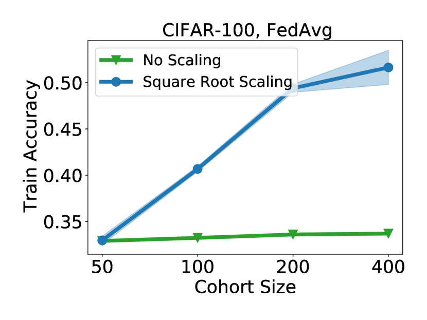
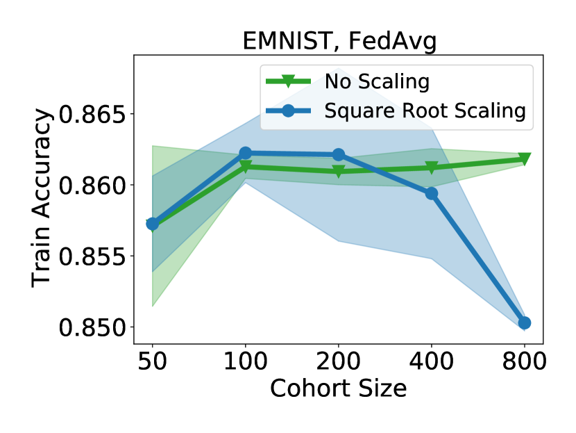
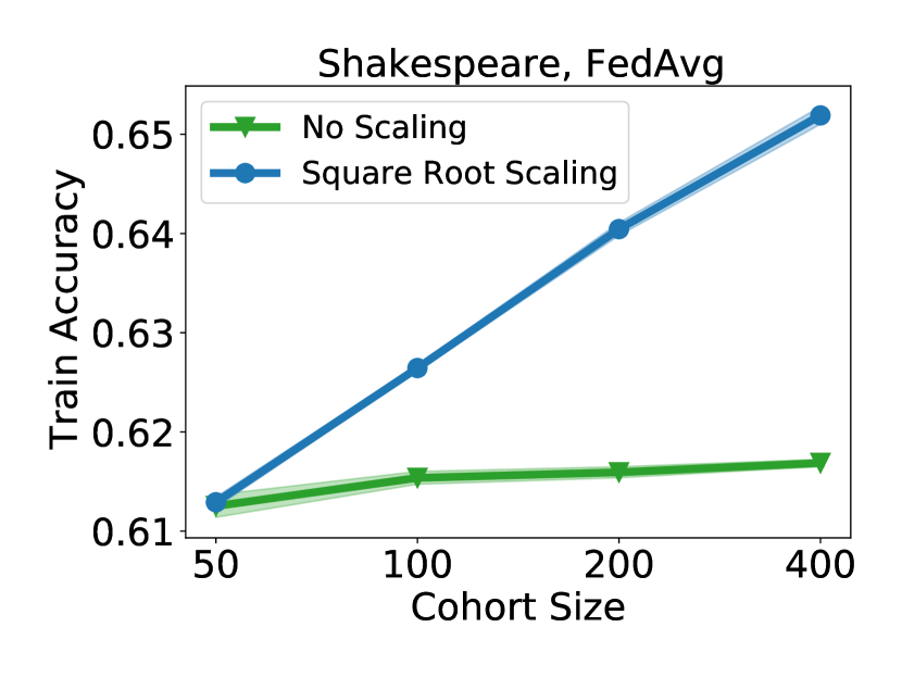
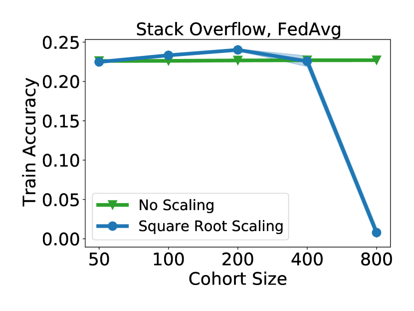
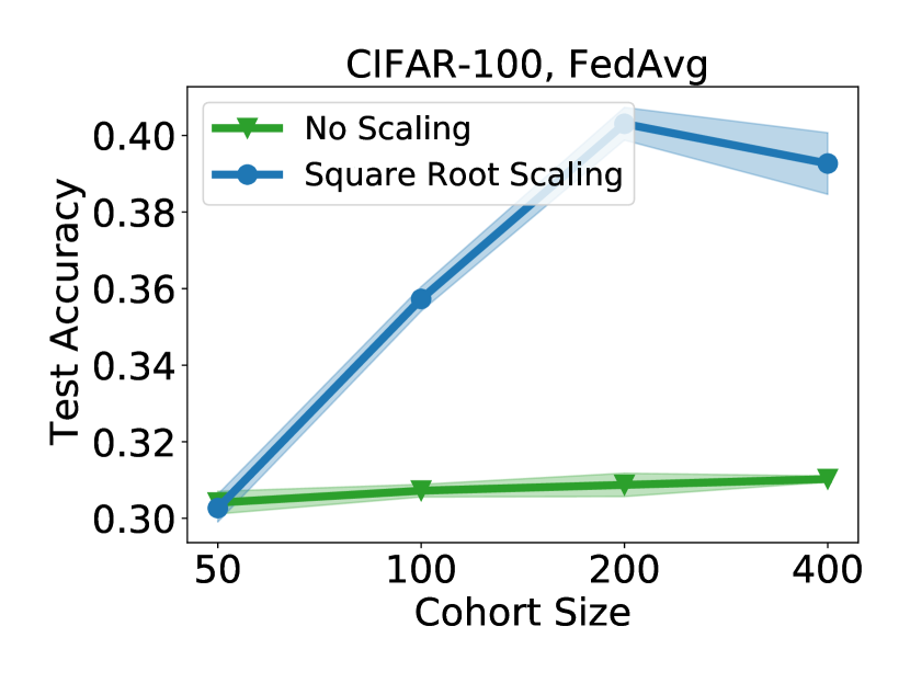
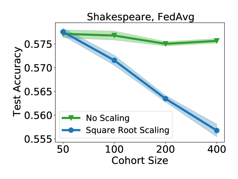
Figure 41: The train accuracy (top) and test accuracy (bottom) of FedAvg using square root scaling with warmup, versus no scaling, after training for 1500 communication rounds. Results are given for various cohort sizes and tasks

B.8 Dynamic Cohort Sizes

In this section, we plot the full results of using the dynamic cohort size strategy from Section 5. Recall that there, we use an analog of dynamic batch size methods for centralized learning, where the cohort size is increased over time. We specifically start with a cohort size of $M=50$, and double every 300 communication rounds. If doubling would ever make the cohort size larger than the number of training clients, we simply use the full set of training clients in a cohort.

We plot the test accuracy of FedAdam and FedAvg using the dynamic cohort size, as well as fixed cohort sizes of $M=50$ and $M=400$ (for CIFAR-100 and Shakespeare) or $M=800$. In Figure 42, the test accuracy is plotted with respect to the number of examples processed by the clients, in order to measure the data-efficiency of the various methods. We find that while the dynamic cohort strategy can help interpolate the data efficiency between small and large cohort sizes, obtaining the same data efficiency as $M=50$ for most accuracy thresholds, then transitioning to the data efficiency of larger $M$.

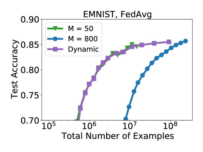
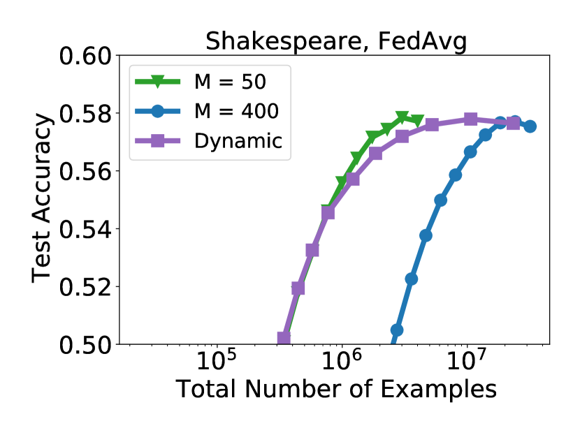
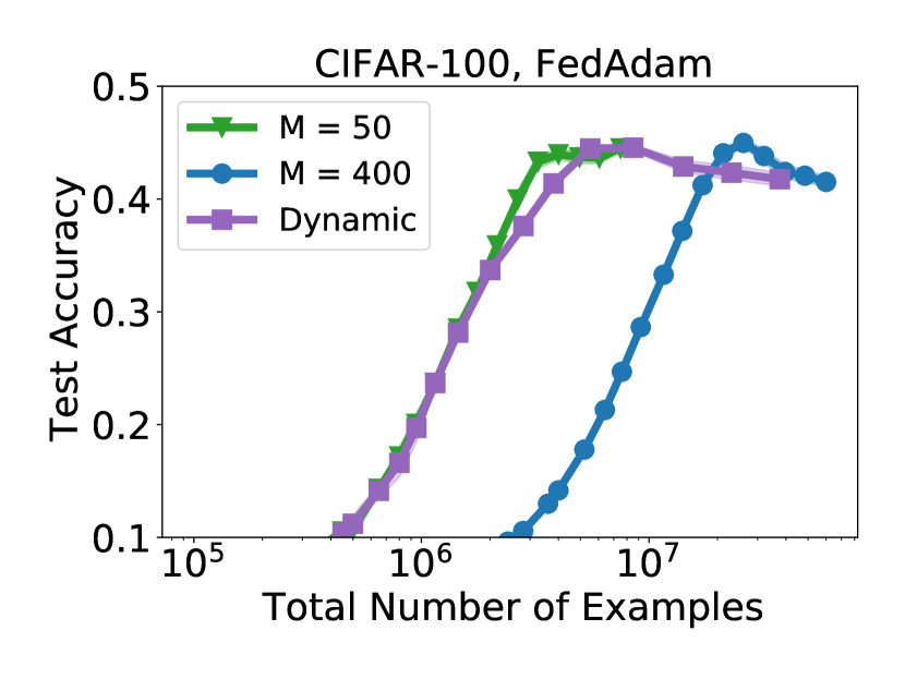
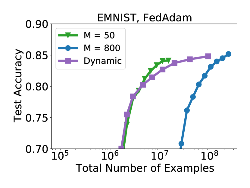
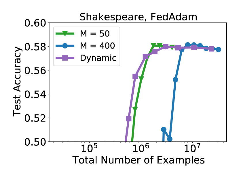
Figure 42: Test accuracy of FedAvg (top) and FedAdam (bottom) with respect to the total number of examples. Both algorithms are applied to various tasks, with various fixed cohort sizes, and the dynamically increasing cohort strategy.

In Figure 43, we plot the test accuracy of the methods discussed above with respect to the number of communication rounds, in order to better visualize the generalization behavior of the dynamic cohort strategy. We see that for FedAvg, there is little to no difference between the test accuracy for $M=50$ and $M=400$ or $M=800$, and that the dynamic cohort strategy generally lays in-between these two. This is partially a consequence of the diminishing returns discussed in Section 3.2. For FedAdam, we see that there are more returns to be had for increasing the cohort size. Moreover, we see that the dynamic cohort strategy typically begins at the accuracy level of $M=50$, and later matches that of the larger cohort. This can be beneficial such as in the case of Stack Overflow, or it can be detrimental as in the case of CIFAR-100, where we see that the dynamic cohort strategy faces the generalization issues in Section 3.3. Thus, we see that the dynamic cohort strategy can help improve the data efficiency of large cohort training, but cannot remedy issues of diminishing returns or generalization failures.

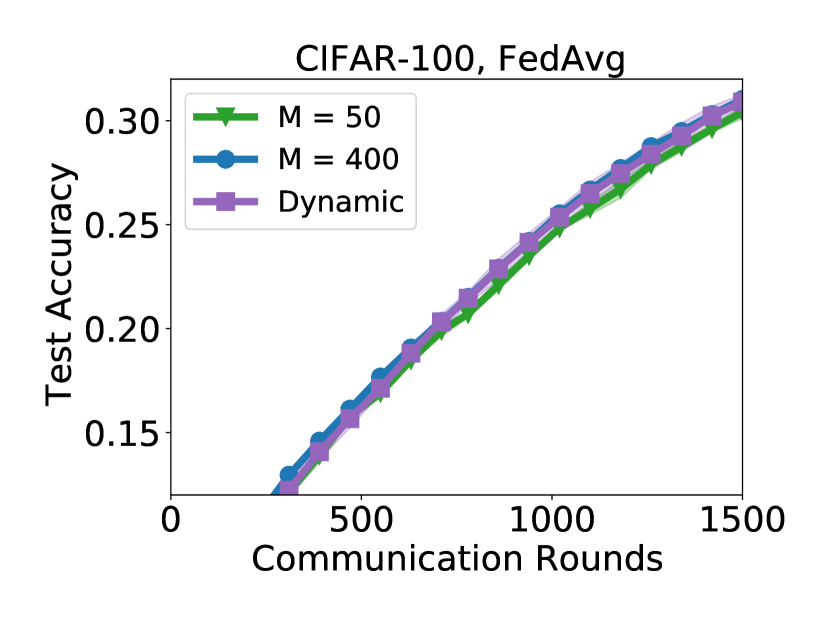
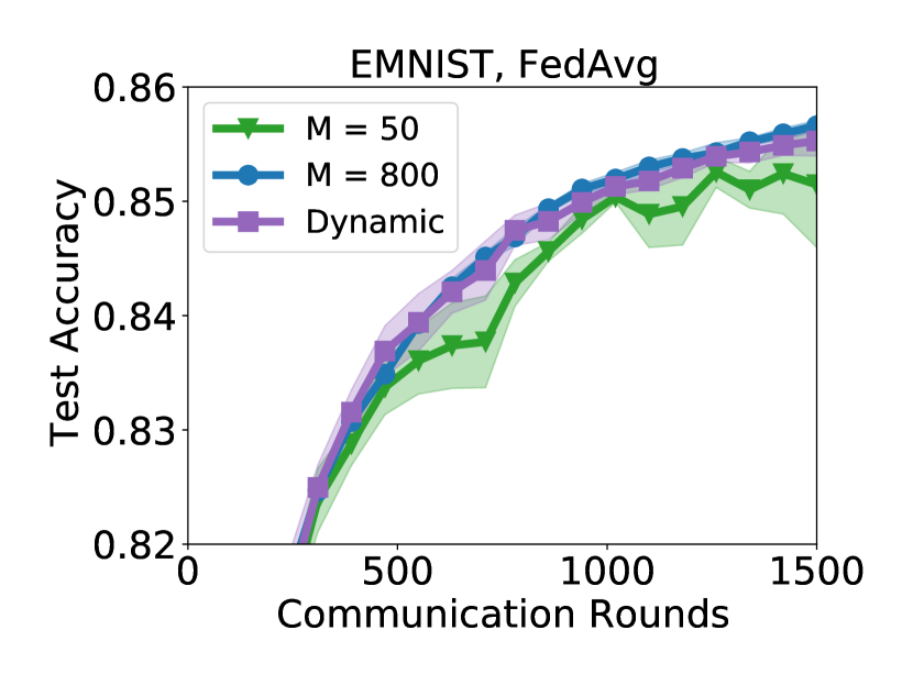
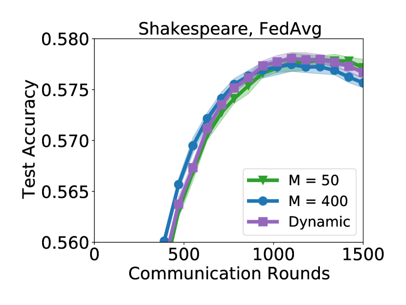
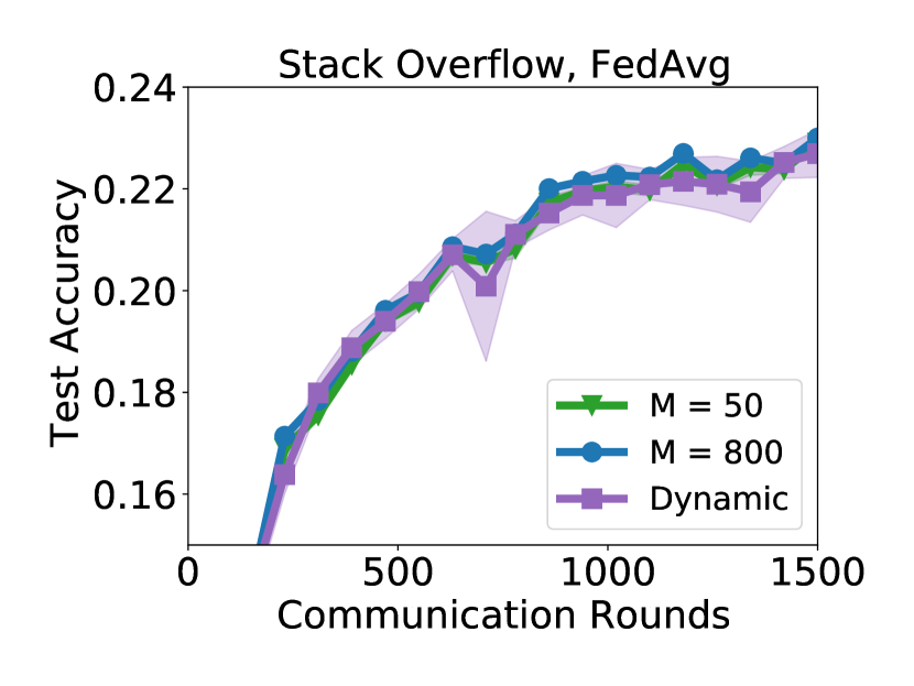
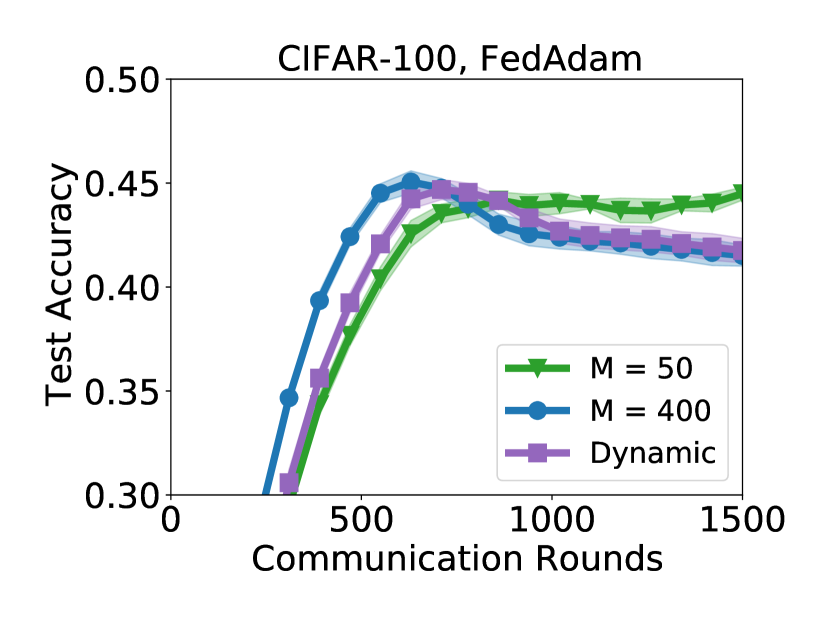
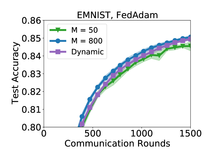
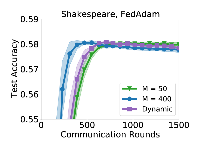
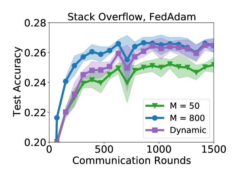
Figure 43: Test accuracy of FedAvg (top) and FedAdam (bottom) with respect to the total number of communication rounds. Both algorithms are applied to various tasks, with various fixed cohort sizes, and the dynamically increasing cohort strategy.

References

- Abadi et al. (2016) Martin Abadi, Andy Chu, Ian Goodfellow, H. Brendan McMahan, Ilya Mironov, Kunal Talwar, and Li Zhang. Deep learning with differential privacy. In Proceedings of the 2016 ACM SIGSAC Conference on Computer and Communications Security, page 308–318, 2016.
- Andrew et al. (2019) Galen Andrew, Om Thakkar, H Brendan McMahan, and Swaroop Ramaswamy. Differentially private learning with adaptive clipping. arXiv preprint arXiv:1905.03871, 2019.
- Authors (2019a) The TensorFlow Federated Authors. TensorFlow Federated Stack Overflow dataset, 2019a. URL https://www.tensorflow.org/federated/api_docs/python/tff/simulation/datasets/stackoverflow/load_data.
- Authors (2019b) The TFF Authors. TensorFlow Federated, 2019b. URL https://www.tensorflow.org/federated.
- Basu et al. (2019) Debraj Basu, Deepesh Data, Can Karakus, and Suhas Diggavi. Qsparse-local-SGD: Distributed SGD with quantization, sparsification and local computations. In Advances in Neural Information Processing Systems, 2019.
- Bittau et al. (2017) Andrea Bittau, Úlfar Erlingsson, Petros Maniatis, Ilya Mironov, Ananth Raghunathan, David Lie, Mitch Rudominer, Ushasree Kode, Julien Tinnes, and Bernhard Seefeld. PROCHLO: Strong privacy for analytics in the crowd. In Proceedings of the 26th Symposium on Operating Systems Principles, pages 441–459, 2017.
- Bonawitz et al. (2019) Keith Bonawitz, Hubert Eichner, Wolfgang Grieskamp, Dzmitry Huba, Alex Ingerman, Vladimir Ivanov, Chloé Kiddon, Jakub Konečný, Stefano Mazzocchi, Brendan McMahan, Timon Van Overveldt, David Petrou, Daniel Ramage, and Jason Roselander. Towards federated learning at scale: System design. In Proceedings of Machine Learning and Systems. Proceedings of MLSys, 2019.
- Caldas et al. (2018) Sebastian Caldas, Peter Wu, Tian Li, Jakub Konečný, H Brendan McMahan, Virginia Smith, and Ameet Talwalkar. LEAF: A benchmark for federated settings. arXiv preprint arXiv:1812.01097, 2018.
- Charles and Konečný (2021) Zachary Charles and Jakub Konečný. Convergence and accuracy trade-offs in federated learning and meta-learning. In Proceedings of The 24th International Conference on Artificial Intelligence and Statistics, 2021.
- Chen et al. (2020) Wenlin Chen, Samuel Horvath, and Peter Richtarik. Optimal client sampling for federated learning. arXiv preprint arXiv:2010.13723, 2020.
- Cheu et al. (2019) Albert Cheu, Adam Smith, Jonathan Ullman, David Zeber, and Maxim Zhilyaev. Distributed differential privacy via shuffling. In Annual International Conference on the Theory and Applications of Cryptographic Techniques, pages 375–403, 2019.
- Cho et al. (2020) Yae Jee Cho, Jianyu Wang, and Gauri Joshi. Client selection in federated learning: Convergence analysis and power-of-choice selection strategies. arXiv preprint arXiv:2010.01243, 2020.
- Cohen et al. (2017) Gregory Cohen, Saeed Afshar, Jonathan Tapson, and Andre Van Schaik. EMNIST: Extending MNIST to handwritten letters. In 2017 International Joint Conference on Neural Networks (IJCNN), pages 2921–2926. IEEE, 2017.
- Dean et al. (2012) Jeffrey Dean, Greg Corrado, Rajat Monga, Kai Chen, Matthieu Devin, Mark Mao, Marc’aurelio Ranzato, Andrew Senior, Paul Tucker, Ke Yang, Quoc Le, and Andrew Ng. Large scale distributed deep networks. In Advances in Neural Information Processing Systems, 2012.
- Duchi et al. (2011) John Duchi, Elad Hazan, and Yoram Singer. Adaptive subgradient methods for online learning and stochastic optimization. Journal of Machine Learning Research, 12(Jul):2121–2159, 2011.
- Erlingsson et al. (2020) Úlfar Erlingsson, Vitaly Feldman, Ilya Mironov, Ananth Raghunathan, Shuang Song, Kunal Talwar, and Abhradeep Thakurta. Encode, shuffle, analyze privacy revisited: Formalizations and empirical evaluation. arXiv preprint arXiv:2001.03618, 2020.
- Girgis et al. (2020) Antonious M Girgis, Deepesh Data, Suhas Diggavi, Peter Kairouz, and Ananda Theertha Suresh. Shuffled model of federated learning: Privacy, communication and accuracy trade-offs. arXiv preprint arXiv:2008.07180, 2020.
- Goetz et al. (2019) Jack Goetz, Kshitiz Malik, Duc Bui, Seungwhan Moon, Honglei Liu, and Anuj Kumar. Active federated learning. arXiv preprint arXiv:1909.12641, 2019.
- Golmant et al. (2018) Noah Golmant, Nikita Vemuri, Zhewei Yao, Vladimir Feinberg, Amir Gholami, Kai Rothauge, Michael W Mahoney, and Joseph Gonzalez. On the computational inefficiency of large batch sizes for stochastic gradient descent. arXiv preprint arXiv:1811.12941, 2018.
- Goyal et al. (2017) Priya Goyal, Piotr Dollár, Ross Girshick, Pieter Noordhuis, Lukasz Wesolowski, Aapo Kyrola, Andrew Tulloch, Yangqing Jia, and Kaiming He. Accurate, large minibatch SGD: Training ImageNet in 1 hour. arXiv preprint arXiv:1706.02677, 2017.
- He et al. (2016) Kaiming He, Xiangyu Zhang, Shaoqing Ren, and Jian Sun. Deep residual learning for image recognition. In Proceedings of the IEEE conference on computer vision and pattern recognition, pages 770–778, 2016.
- Hochreiter and Schmidhuber (1997) Sepp Hochreiter and Jürgen Schmidhuber. Long short-term memory. Neural Computation, 9(8):1735–1780, 1997.
- Hoffer et al. (2017) Elad Hoffer, Itay Hubara, and Daniel Soudry. Train longer, generalize better: closing the generalization gap in large batch training of neural networks. In Advances in Neural Information Processing Systems, 2017.
- Hsieh et al. (2020) Kevin Hsieh, Amar Phanishayee, Onur Mutlu, and Phillip Gibbons. The non-IID data quagmire of decentralized machine learning. In Proceedings of the 37th International Conference on Machine Learning, 2020.
- Hsu et al. (2019) Tzu-Ming Harry Hsu, Hang Qi, and Matthew Brown. Measuring the effects of non-identical data distribution for federated visual classification. arXiv preprint arXiv:1909.06335, 2019.
- Hu et al. (2020) Zeou Hu, Kiarash Shaloudegi, Guojun Zhang, and Yaoliang Yu. FedMGDA+: Federated learning meets multi-objective optimization. arXiv preprint arXiv:2006.11489, 2020.
- Kairouz et al. (2021) Peter Kairouz, H. Brendan McMahan, and contributors. Advances and open problems in federated learning. Foundations and Trends® in Machine Learning, 14(1), 2021. ISSN 1935-8237.
- Karimireddy et al. (2020a) Sai Praneeth Karimireddy, Martin Jaggi, Satyen Kale, Mehryar Mohri, Sashank J Reddi, Sebastian U Stich, and Ananda Theertha Suresh. Mime: Mimicking centralized stochastic algorithms in federated learning. arXiv preprint arXiv:2008.03606, 2020a.
- Karimireddy et al. (2020b) Sai Praneeth Karimireddy, Satyen Kale, Mehryar Mohri, Sashank Reddi, Sebastian Stich, and Ananda Theertha Suresh. SCAFFOLD: Stochastic controlled averaging for federated learning. In Proceedings of the 37th International Conference on Machine Learning, 2020b.
- Keskar et al. (2017) Nitish Shirish Keskar, Dheevatsa Mudigere, Jorge Nocedal, Mikhail Smelyanskiy, and Ping Tak Peter Tang. On large-batch training for deep learning: Generalization gap and sharp minima. In International Conference on Learning Representations, 2017.
- Khaled et al. (2019) Ahmed Khaled, Konstantin Mishchenko, and Peter Richtárik. First analysis of local GD on heterogeneous data. arXiv preprint arXiv:1909.04715, 2019.
- Khaled et al. (2020) Ahmed Khaled, Konstantin Mishchenko, and Peter Richtarik. Tighter theory for local SGD on identical and heterogeneous data. In Proceedings of the Twenty Third International Conference on Artificial Intelligence and Statistics, 2020.
- Kingma and Ba (2015) Diederik P. Kingma and Jimmy Ba. Adam: A method for stochastic optimization. In International Conference on Learning Representations, 2015.
- Konečnỳ et al. (2016) Jakub Konečnỳ, H Brendan McMahan, Daniel Ramage, and Peter Richtárik. Federated optimization: Distributed machine learning for on-device intelligence. arXiv preprint arXiv:1610.02527, 2016.
- Krizhevsky (2009) Alex Krizhevsky. Learning multiple layers of features from tiny images. Technical report, 2009.
- Krizhevsky (2014) Alex Krizhevsky. One weird trick for parallelizing convolutional neural networks. arXiv preprint arXiv:1404.5997, 2014.
- Laguel et al. (2021) Yassine Laguel, Krishna Pillutla, Jerôme Malick, and Zaid Harchaoui. A superquantile approach to federated learning with heterogeneous devices. In 2021 55th Annual Conference on Information Sciences and Systems (CISS), 2021.
- Lee et al. (2017) Kangwook Lee, Maximilian Lam, Ramtin Pedarsani, Dimitris Papailiopoulos, and Kannan Ramchandran. Speeding up distributed machine learning using codes. IEEE Transactions on Information Theory, 64(3):1514–1529, 2017.
- Li and Wang (2019) Daliang Li and Junpu Wang. FedMD: Heterogenous federated learning via model distillation. arXiv preprint arXiv:1910.03581, 2019.
- Li et al. (2019) Tian Li, Anit Kumar Sahu, Manzil Zaheer, Maziar Sanjabi, Ameet Talwalkar, and Virginia Smithy. FedDANE: A federated newton-type method. In 2019 53rd Asilomar Conference on Signals, Systems, and Computers, pages 1227–1231. IEEE, 2019.
- Li et al. (2020a) Tian Li, Anit Kumar Sahu, Ameet Talwalkar, and Virginia Smith. Federated learning: Challenges, methods, and future directions. IEEE Signal Processing Magazine, 37(3):50–60, 2020a.
- Li et al. (2020b) Tian Li, Anit Kumar Sahu, Manzil Zaheer, Maziar Sanjabi, Ameet Talwalkar, and Virginia Smith. Federated optimization in heterogeneous networks. In Proceedings of Machine Learning and Systems 2020, pages 429–450, 2020b.
- Li et al. (2020c) Tian Li, Maziar Sanjabi, Ahmad Beirami, and Virginia Smith. Fair resource allocation in federated learning. In International Conference on Learning Representations, 2020c.
- Li and McCallum (2006) Wei Li and Andrew McCallum. Pachinko allocation: DAG-structured mixture models of topic correlations. In Proceedings of the 23rd International Conference on Machine Learning, 2006.
- Liang and Kozat (2014) Guanfeng Liang and Ulaş C Kozat. Tofec: Achieving optimal throughput-delay trade-off of cloud storage using erasure codes. In IEEE INFOCOM 2014-IEEE Conference on Computer Communications, 2014.
- Lin et al. (2019) Tao Lin, Sebastian U Stich, Kumar Kshitij Patel, and Martin Jaggi. Don’t use large mini-batches, use local SGD. In International Conference on Learning Representations, 2019.
- Lin et al. (2020) Tao Lin, Lingjing Kong, Sebastian Stich, and Martin Jaggi. Extrapolation for large-batch training in deep learning. In Proceedings of the 37th International Conference on Machine Learning, 2020.
- Ma et al. (2018) Siyuan Ma, Raef Bassily, and Mikhail Belkin. The power of interpolation: Understanding the effectiveness of SGD in modern over-parametrized learning. In Proceedings of the 35th International Conference on Machine Learning, 2018.
- Malinovskiy et al. (2020) Grigory Malinovskiy, Dmitry Kovalev, Elnur Gasanov, Laurent Condat, and Peter Richtarik. From local SGD to local fixed-point methods for federated learning. In Proceedings of the 37th International Conference on Machine Learning, 2020.
- Masters and Luschi (2018) Dominic Masters and Carlo Luschi. Revisiting small batch training for deep neural networks. arXiv preprint arXiv:1804.07612, 2018.
- McCandlish et al. (2018) Sam McCandlish, Jared Kaplan, Dario Amodei, and OpenAI Dota Team. An empirical model of large-batch training. arXiv preprint arXiv:1812.06162, 2018.
- McMahan et al. (2017) Brendan McMahan, Eider Moore, Daniel Ramage, Seth Hampson, and Blaise Aguera y Arcas. Communication-efficient learning of deep networks from decentralized data. In Proceedings of the 20th International Conference on Artificial Intelligence and Statistics, volume 54, 2017.
- McMahan and Streeter (2010) H. Brendan McMahan and Matthew J. Streeter. Adaptive bound optimization for online convex optimization. In COLT The 23rd Conference on Learning Theory, 2010.
- McMahan et al. (2018) H. Brendan McMahan, Daniel Ramage, Kunal Talwar, and Li Zhang. Learning differentially private recurrent language models. In International Conference on Learning Representations, 2018.
- Mikolov et al. (2010) Tomáš Mikolov, Martin Karafiát, Lukáš Burget, Jan Černockỳ, and Sanjeev Khudanpur. Recurrent neural network based language model. In Eleventh Annual Conference of the International Speech Communication Association, 2010.
- Mohri et al. (2019) Mehryar Mohri, Gary Sivek, and Ananda Theertha Suresh. Agnostic federated learning. In Proceedings of the 36th International Conference on Machine Learning, 2019.
- Nacson et al. (2019) Mor Shpigel Nacson, Jason Lee, Suriya Gunasekar, Pedro Henrique Pamplona Savarese, Nathan Srebro, and Daniel Soudry. Convergence of gradient descent on separable data. In The 22nd International Conference on Artificial Intelligence and Statistics, 2019.
- Nishio and Yonetani (2019) Takayuki Nishio and Ryo Yonetani. Client selection for federated learning with heterogeneous resources in mobile edge. In IEEE International Conference on Communications (ICC), 2019.
- Pathak and Wainwright (2020) Reese Pathak and Martin J Wainwright. FedSplit: An algorithmic framework for fast federated optimization. In Advances in Neural Information Processing Systems, pages 7057–7066, 2020.
- Paulik et al. (2021) Matthias Paulik, Matt Seigel, Henry Mason, Dominic Telaar, Joris Kluivers, Rogier van Dalen, Chi Wai Lau, Luke Carlson, Filip Granqvist, Chris Vandevelde, et al. Federated evaluation and tuning for on-device personalization: System design & applications. arXiv preprint arXiv:2102.08503, 2021.
- Reddi et al. (2021) Sashank J. Reddi, Zachary Charles, Manzil Zaheer, Zachary Garrett, Keith Rush, Jakub Konečný, Sanjiv Kumar, and Hugh Brendan McMahan. Adaptive federated optimization. In International Conference on Learning Representations, 2021.
- Ribero and Vikalo (2020) Monica Ribero and Haris Vikalo. Communication-efficient federated learning via optimal client sampling. arXiv preprint arXiv:2007.15197, 2020.
- Shallue et al. (2019) Christopher J Shallue, Jaehoon Lee, Joseph Antognini, Jascha Sohl-Dickstein, Roy Frostig, and George E Dahl. Measuring the effects of data parallelism on neural network training. Journal of Machine Learning Research, 20:1–49, 2019.
- Shi et al. (2011) Elaine Shi, TH Hubert Chan, Eleanor Rieffel, Richard Chow, and Dawn Song. Privacy-preserving aggregation of time-series data. In Proc. NDSS, volume 2, pages 1–17, 2011.
- Smith et al. (2018) Samuel L. Smith, Pieter-Jan Kindermans, and Quoc V. Le. Don’t decay the learning rate, increase the batch size. In International Conference on Learning Representations, 2018.
- Wang et al. (2020) Hongyi Wang, Mikhail Yurochkin, Yuekai Sun, Dimitris Papailiopoulos, and Yasaman Khazaeni. Federated learning with matched averaging. In International Conference on Learning Representations, 2020.
- Wu and He (2018) Yuxin Wu and Kaiming He. Group normalization. In Proceedings of the European Conference on Computer Vision (ECCV), pages 3–19, 2018.
- Yang et al. (2021) Haibo Yang, Minghong Fang, and Jia Liu. Achieving linear speedup with partial worker participation in non-IID federated learning. In International Conference on Learning Representations, 2021.
- Yin et al. (2018) Dong Yin, Ashwin Pananjady, Max Lam, Dimitris Papailiopoulos, Kannan Ramchandran, and Peter Bartlett. Gradient diversity: a key ingredient for scalable distributed learning. In Proceedings of the Twenty-First International Conference on Artificial Intelligence and Statistics, 2018.
- You et al. (2017) Yang You, Igor Gitman, and Boris Ginsburg. Large batch training of convolutional networks. arXiv preprint arXiv:1708.03888, 2017.
- You et al. (2020) Yang You, Jing Li, Sashank Reddi, Jonathan Hseu, Sanjiv Kumar, Srinadh Bhojanapalli, Xiaodan Song, James Demmel, Kurt Keutzer, and Cho-Jui Hsieh. Large batch optimization for deep learning: Training bert in 76 minutes. In International Conference on Learning Representations, 2020.
- Zhang et al. (2020) Xinwei Zhang, Mingyi Hong, Sairaj Dhople, Wotao Yin, and Yang Liu. FedPD: A federated learning framework with optimal rates and adaptivity to non-IID data. arXiv preprint arXiv:2005.11418, 2020.