Tree-Values: selective inference for regression trees
Abstract
We consider conducting inference on the output of the Classification and Regression Tree (CART) [Breiman et al., 1984] algorithm. A naive approach to inference that does not account for the fact that the tree was estimated from the data will not achieve standard guarantees, such as Type 1 error rate control and nominal coverage. Thus, we propose a selective inference framework for conducting inference on a fitted CART tree. In a nutshell, we condition on the fact that the tree was estimated from the data. We propose a test for the difference in the mean response between a pair of terminal nodes that controls the selective Type 1 error rate, and a confidence interval for the mean response within a single terminal node that attains the nominal selective coverage. Efficient algorithms for computing the necessary conditioning sets are provided. We apply these methods in simulation and to a dataset involving the association between portion control interventions and caloric intake.
1 Introduction
Regression tree algorithms recursively partition covariate space using binary splits to obtain regions that are maximally homogeneous with respect to a continuous response. The Classification and Regression Tree (CART; Breiman et al. 1984) proposal, which involves growing a large tree and then pruning it back, is by far the most popular of these algorithms.
The regions defined by the splits in a fitted CART tree induce a piecewise constant regression model where the predicted response within each region is the mean of the observations in that region. CART is popular in large part because it is highly interpretable; someone without technical expertise can easily “read” the tree to make predictions, and to understand why a certain prediction is made. However, its interpretability belies the fact that CART trees are highly unstable: a small change to the training dataset can drastically change the structure of the fitted tree. In the absence of an established notion of statistical significance associated with a given split in the tree, it is hard for a practitioner to know whether they are interpreting signal or noise. In this paper, we use the framework of selective inference to fill this gap by providing a toolkit to conduct inference on hypotheses motivated by the output of the CART algorithm.
Given a CART tree, consider testing for a difference in the mean response of the regions resulting from a binary split. A very naive approach, such as a two-sample -test, that does not account for the fact that the regions were themselves estimated from the data will fail to control the selective Type 1 error rate: the probability of rejecting a true null hypothesis, given that we decided to test it [Fithian et al., 2014]. Similarly, a naive -interval for the mean response in a region will not attain nominal selective coverage: the probability that the interval covers the parameter, given that we chose to construct it.
In fact, approaches for conducting inference on the output of a regression tree are quite limited. Sample splitting involves fitting a CART tree using a subset of the observations, which will naturally lead to an inferior tree to the one resulting from all of the observations, and thus is unsatisfactory in many applied settings; see Athey and Imbens [2016]. Wager and Walther [2015] develop convergence guarantees for unpruned CART trees that can be leveraged to build confidence intervals for the mean response within a region; however, they do not provide finite-sample results and cannot accommodate pruning. Loh et al. [2016] and Loh et al. [2019] develop bootstrap calibration procedures that attempt to provide confidence intervals for the regions of a regression tree. In Appendix A, we show that this bootstrap calibration approach fails to provide intervals that achieve nominal coverage for the parameters of interest in this paper.
As an alternative to performing inference on a CART tree, one could turn to the conditional inference tree (CTree) framework of Hothorn et al. [2006]. This framework uses a different tree-growing algorithm than CART, and at each split tests for linear association between the split covariate and the response. As summarized in Loh [2014], the CTree framework alleviates issues with instability and variable selection bias associated with CART. Despite these advantages, CTree remains far less widely-used than CART. Furthermore, while CTree attaches a notion of statistical significance to each split in a tree, it does not directly allow for inference on the mean response within a region or the difference in mean response between two regions. Finally, while the CTree framework requires few assumptions, its inference is based on asymptotics.
In this paper, we introduce a finite-sample selective inference [Fithian et al., 2014] framework for the difference between the mean responses in two regions, and for the mean response in a single region, in a pruned or unpruned CART tree. We condition on the event that CART yields a particular set of regions, and thereby achieve selective Type 1 error rate control as well as nominal selective coverage.
The rest of this paper is organized as follows. In Section 2, we review the CART algorithm, and briefly define some key ideas in selective inference. In Section 3, we present our proposal for selective inference on the regions estimated via CART. We show that the necessary conditioning sets can be efficiently computed in Section 4. In Section 5 we compare our framework to sample splitting and CTree via simulation. In Section 6 we compare our framework to CTree on data from the Box Lunch Study. The discussion is in Section 7. Technical details are relegated to the supplementary materials.
2 Background
2.1 Notation for Regression Trees
Given covariates measured on each of observations , let denote the th order statistic of the th covariate, and define the half-spaces
| (1) |
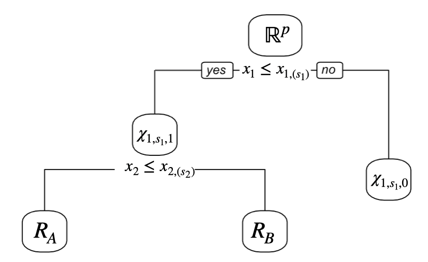
The following definitions are illustrated in Figure 1.
Definition 1 (Tree and Region).
Consider a set such that for all . Then is a tree if and only if (i) ; (ii) every element of equals for some , , , ; (iii) implies that for ; and (iv) for any . If and is a tree, then we refer to as a region.
We use the notation to refer to a particular tree. Definition 1 implies that any region is of the form , where for each , we have that , , and . We call the level of the region, and use the convention that the level of is .
Definition 2 (Siblings and Children).
Suppose that . Then and are siblings. Furthermore, they are the children of .
Definition 3 (Descendant and Ancestor).
If and , then is a descendant of , and is an ancestor of .
Definition 4 (Terminal Region).
A region without descendants is a terminal region.
We let denote the set of descendants of region in , and we let denote the subset of that are terminal regions.
Given a response vector , let , where is an indicator variable that equals if the event holds, and otherwise. Then, a tree induces the regression model . In other words, it predicts the response within each terminal region to be the mean of the observations in that region.
2.2 A Review of the CART Algorithm [Breiman et al., 1984]
The CART algorithm [Breiman et al., 1984] greedily searches for a tree that minimizes the sum of squared errors . It first grows a very large tree via recursive binary splits, starting with the full covariate space . To split a region , it selects the covariate and the split point to maximize the gain, defined as
| (2) |
Details are provided in Algorithm A1.
Once a very large tree has been grown, cost-complexity pruning is applied. We define the average per-region gain in sum-of-squared errors provided by the descendants of a region ,
| (3) |
Given a complexity parameter , if for some , then cost-complexity pruning removes ’s descendants from , turning into a terminal region. Details are in Algorithm A2, which involves the notion of a bottom-up ordering.
Definition 5 (Bottom-up ordering).
Let . Let be a permutation of the integers . Then is a bottom-up ordering of the regions in if, for all , if .
There are other equivalent formulations for cost-complexity pruning (see Proposition 7.2 in Ripley [1996]); the formulation in Algorithm A2 is convenient for establishing the results in this paper.
To summarize, the CART algorithm first applies Algorithm A1 to the initial region and the data to obtain an unpruned tree, which we call . It then applies Algorithm A2 to to obtain an optimally-pruned tree using complexity parameter , which we call .
Algorithm A1 (Growing a tree).
Grow(, )
| 1. If a stopping condition is met, return . |
| 2. Else return Grow(), Grow(, ), where |
Algorithm A2 (Cost-complexity pruning).
Parameter is a bottom-up ordering of the regions in .
Prune(, , , )
| 1. Let . Let be the number of regions in . |
| 2. For : |
| (a) Let be the th region in . |
| (b) Update as follows, where is defined in (3): |
| 3. Return . |
2.3 A Brief Overview of Selective Inference
Here, we provide a very brief overview of selective inference; see Fithian et al. [2014] or Taylor and Tibshirani [2015] for a more detailed treatment.
Consider conducting inference on a parameter . Classical approaches assume that we were already interested in conducting inference on before looking at our data. If, instead, our interest in was sparked by looking at our data, then inference must be performed with care: we must account for the fact that we “selected” based on the data [Fithian et al., 2014]. In this setting, interest focuses on a p-value such that the test for based on controls the selective Type 1 error rate, in the sense that
| (4) |
Also of interest are confidence intervals that achieve -selective coverage for the parameter , meaning that
| (5) |
Roughly speaking, the inferential guarantees in (4) and (5) can be achieved by defining p-values and confidence intervals that condition on the aspect of the data that led to the selection of . In recent years, a number of papers have taken this approach to perform selective inference on parameters selected from the data in the regression [Lee et al., 2016, Liu et al., 2018, Tian and Taylor, 2018, Tibshirani et al., 2016], clustering [Gao et al., 2020], and changepoint detection [Hyun et al., 2021, Jewell et al., 2022] settings.
3 The Selective Inference Framework for CART
3.1 Inference on a Pair of Sibling Regions
Throughout this paper, we assume that with known.
We let denote a fixed covariate matrix. Suppose that we apply CART with complexity parameter to a realization from to obtain . Given sibling regions and in , we define a contrast vector such that
| (6) |
and . Now, consider testing the null hypothesis of no difference in means between and , i.e. . This null hypothesis is of interest because and appeared as siblings in . A test based on a p-value of the form that does not account for this will not control the selective Type 1 error rate in (4).
To control the selective Type 1 error rate, we propose a p-value that conditions on the aspect of the data that led us to select ,
| (7) |
But (7) depends on a nuisance parameter, the portion of that is orthogonal to . To remove the dependence on this nuisance parameter, we condition on its sufficient statistic , where . The resulting p-value, or “tree-value”, is defined as
| (8) |
Results similar to Theorem 1 can be found in Jewell et al. [2022], Lee et al. [2016], Liu et al. [2018], and Tibshirani et al. [2016].
Theorem 1.
Proofs of all theoretical results are provided in the appendix. Theorem 1 says that given the set , we can compute the p-value in (8) using
| (11) |
where denotes the cumulative distribution function of the distribution truncated to the set . In Section 4, we provide an efficient approach for analytically characterizing the truncation set . To avoid numerical issues associated with the truncated normal distribution, we compute (11) using methods described in the supplement of Chen and Bien [2020]. Note that the proof of Theorem 1, and consequently the efficient computation of discussed in Section 4, relies on the assumption that .
We now consider inverting the test proposed in (8) to construct an equitailed confidence interval for that has -selective coverage (5), in the sense that
| (12) |
Proposition 1.
For any and any realization , the values and that satisfy
| (13) |
are unique, and achieves -selective coverage for .
3.2 Inference on a Single Region
Given a single region in a CART tree, we define the contrast vector such that
| (14) |
Then, . We now consider testing the null hypothesis for some fixed . Because our interest in this null hypothesis results from the fact that , we must condition on this event in defining the p-value. We define
| (15) |
and introduce the following theorem.
Theorem 2.
Theorem 2 and the resulting efficient computations in Section 4 rely on the assumption that .
We can also define a confidence interval for that attains nominal selective coverage.
Proposition 2.
For any and any realization , the values and that satisfy
| (17) |
are unique, and achieves -selective coverage for .
3.3 Intuition for the Conditioning Sets and
We first develop intuition for the set defined in (10). From Theorem 1,
Thus, is a perturbation of that exaggerates the difference between the observed sample mean responses of and if , and shrinks that difference if . The set quantifies the amount that we can shift the difference in sample mean responses between and while still producing a tree containing these sibling regions. The top row of Figure 2 displays , as a function of , in an example where .
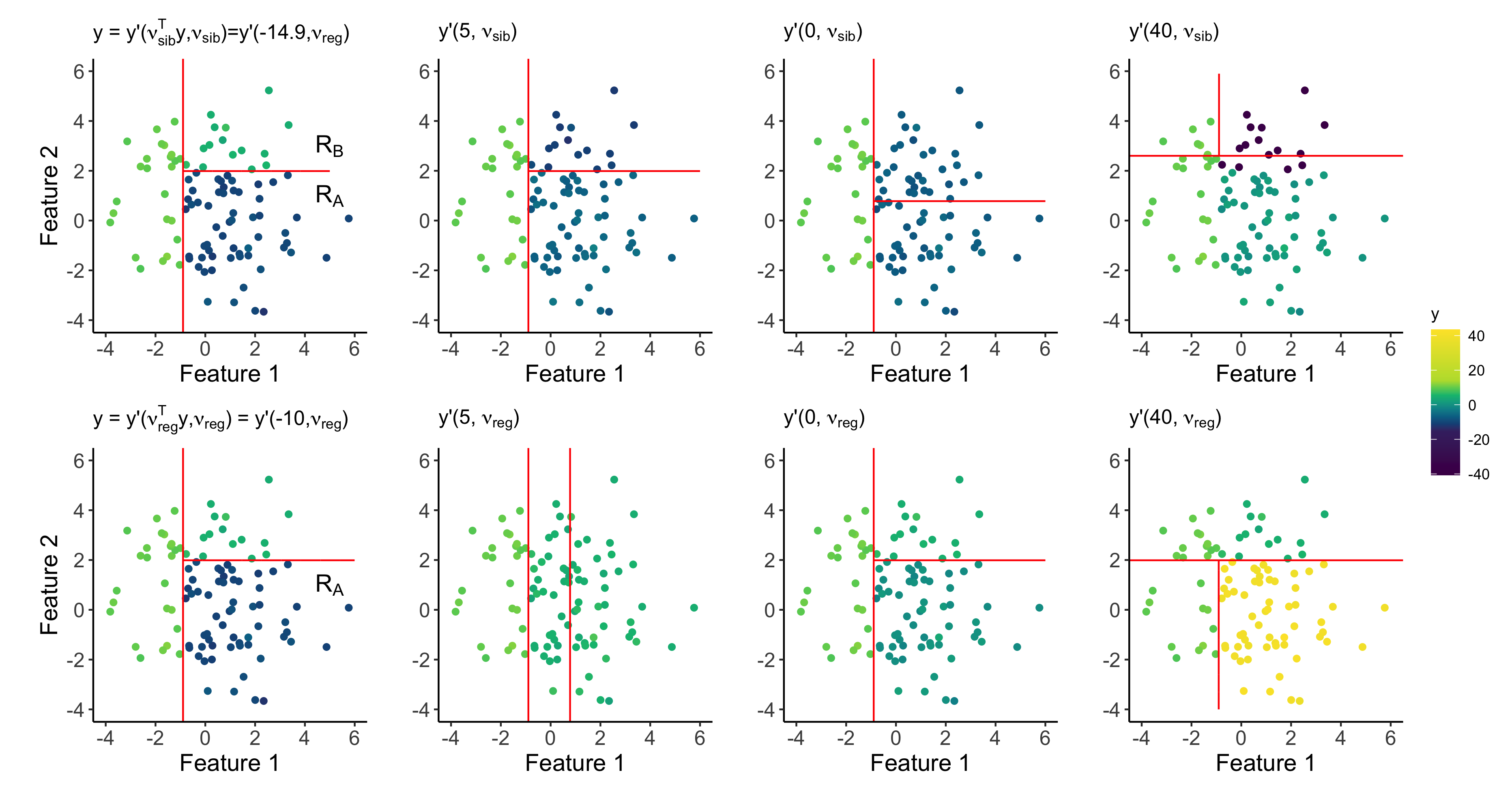
We next develop intuition for , defined in (16). Note that , where is defined in Theorem 2. Thus, shifts the responses of the observations in so that their sample mean equals , and leaves the others unchanged. The set quantifies the amount that we can exaggerate or shrink the sample mean response in region while still producing a tree that contains . The bottom row of Figure 2 displays as is varied, in an example with .
4 Computing the conditioning sets and
4.1 Recharacterizing the conditioning sets in terms of branches
We begin by introducing the concept of a branch.
Definition 6 (Branch).
A branch is an ordered sequence of triples such that , , and for . The branch induces a nested set of regions , where for , and .
For a branch and a vector , we define
| (18) |
For , we let denote the branch such that contains and all of its ancestors in .
Lemma 1.
Lemma 1 says that contains siblings and if and only if it contains the entire branch associated with in . However, Lemma 1 does not apply in the single region case: for defined in (14) and some , the fact that does not imply that . Instead, a result similar to Lemma 1 holds, involving permutations of the branch.
Definition 7 (Permutation of a branch).
Let denote the set of all permutations of . Given and a branch , we say that is a permutation of the branch .
Branch and its permutation induce the same region , but .
Lemma 2.
Let . Then if and only if there exists a such that . Thus, for in (16),
| (19) |
4.2 Computing in (18)
Throughout this section, we consider a vector and a branch , where may or may not be in . Recall from Definition 6 that induces the nested regions for , and . Throughout this section, our only requirement on and is the following condition.
Condition 1.
For defined in Theorem 1, and satisfy for and for some constants and .
To characterize in (18), recall that the CART algorithm in Section 2.2 involves growing a very large tree , and then pruning it. We first characterize the set
| (20) |
Proposition 3.
Recall the definition of in (2), and let Then,
Proposition 4 says that we can compute efficiently.
Proposition 4.
The set is defined by a quadratic inequality in . Furthermore, we can evaluate all of the sets , for , , , in operations. Intersecting these sets to obtain requires at most operations, and only operations if and is of the form in (6).
Noting that , it remains to characterize the set of such that is not removed during pruning. Recall that was defined in (3).
Proposition 5.
We explain how to compute a satisfying (21) when in the supplementary materials.
Proposition 6.
The set in (21) is the intersection of the solution sets of quadratic inequalities in . Given , the coefficients of these quadratics can be obtained in operations. After has been computed, intersecting it with these quadratic sets to obtain from (21) requires operations in general, and only operations if and from (6).
The results in this section have relied upon Condition 1. Indeed, this condition holds for branches and vectors that arise in characterizing the sets and .
Proposition 7.
Combining Lemma 1 with Propositions 3–7, we see that can be computed in operations.
However, computing is much more computationally intensive: by Lemma 2 and Propositions 3–7, it requires computing
for all permutations , for a total of operations. In Section 4.3, we discuss ways to avoid these calculations.
4.3 A Computationally-Efficient Alternative to
Lemma 2 suggests that carrying out
inference on a single region requires computing
for every . We now present a less computationally demanding alternative.
Proposition 8.
Let be a subset of the permutations in , i.e. . Define
The test based on controls the selective Type 1 error rate (4) for . Furthermore, , where .
Using the notation in Proposition 8, introduced in (15) equals . If we take , where is the identity permutation, then we arrive at
| (22) |
where . The set can be easily computed by Proposition 5.
Compared to (15), (22) conditions on an extra piece of information: the ancestors of . Thus, while (22) controls the selective Type 1 error rate, it may have lower power than (15) [Fithian et al., 2014]. Similarly, inverting (22) to form a confidence interval provides correct selective coverage, but may yield intervals that are wider than those in Proposition 2. Proposition 8 is motivated by a proposal by Lee et al. [2016] to condition on both the selected model (necessary information) and the signs of the selected variables (extra information) in the lasso setting, to gain computational efficiency at the possible expense of precision and power.
In Appendix F, we show through simulation that the loss in power associated with using (22) rather than (15) is negligible. Thus, in practice, we suggest using (22) for its computational efficiency. We use (22) for the remainder of this paper.
Furthermore, we can consider computing confidence intervals of the form rather than (17), where and satisfy
| (23) |
In Appendix F, we show that the confidence intervals resulting from (4.3) are not much wider than those resulting from (17). We therefore make use of confidence intervals of the form (4.3) in the remainder of this paper.
5 Simulation Study
5.1 Data Generating Mechanism
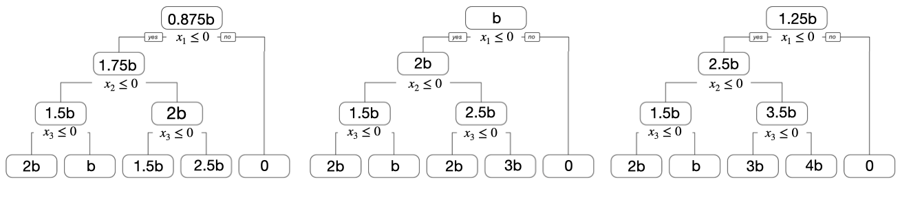
We simulate with , and with and . This vector defines a three-level tree, shown in Figure 3 for three values of .
5.2 Methods for Comparison
All CART trees are fit using the R package rpart [Therneau and Atkinson, 2019] with , a maximum level of three, and a minimum node size of one. We compare three approaches for conducting inference. (i) Selective -methods: Fit a CART tree to the data. For each split, test for a difference in means between the two sibling regions using (8), and compute the corresponding confidence interval in (13). Compute the confidence interval for the mean of each region using (4.3). (ii) Naive -methods: Fit a CART tree to the data. For each split, conduct a naive -test for the difference in means between the two sibling regions, and compute the corresponding naive -interval. Compute a naive -interval for each region’s mean. (iii) Sample splitting: Split the data into equally-sized training and test sets. Fit a CART tree to the training set. On the test set, conduct a naive -test for each split and compute a naive -interval for each split and each region. If a region has no test set observations, then we fail to reject the null hypothesis and fail to cover the parameter.
The conditional inference tree (CTree) framework of Hothorn et al. [2006] uses a different criterion than CART to perform binary splits. Within a region, it tests for linear association between each covariate and the response. The covariate with the smallest p-value for this linear association is selected as the split variable, and a Bonferroni corrected p-value that accounts for the number of covariates is reported in the final tree. Then, the split point is selected. If, after accounting for multiple testing, no variable has a p-value below a pre-specified significance level , then the recursion stops. While CTree’s p-values assess linear association and thus are not directly comparable to the p-values in (i)–(iii) above, it is the most popular framework currently available for determining if a regression tree split is statistically significant. Thus, we also evaluate the performance of (iv) CTree: Fit a CTree to all of the data using the R package partykit [Hothorn and Zeileis, 2015] with . For each split, record the p-value reported by partykit.
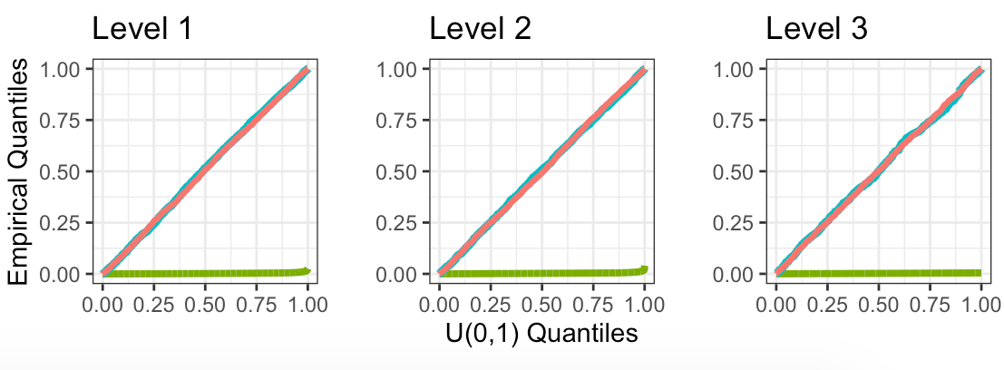
5.3 Uniform p-values under a Global Null
We generate datasets with , so that holds for all splits in all trees. Figure 4 displays the distributions of p-values across all splits in all fitted trees for the naive -test, sample splitting, and the selective -test. The selective -test and sample splitting achieve uniform p-values under the null, while the naive -test (which does not account for the fact that was obtained by applying CART to the same data used for testing) does not. CTree is omitted from the comparison: it creates a split only if the p-value is less than , and thus its p-values over the splits do not follow a Uniform(0,1) distribution.
5.4 Power
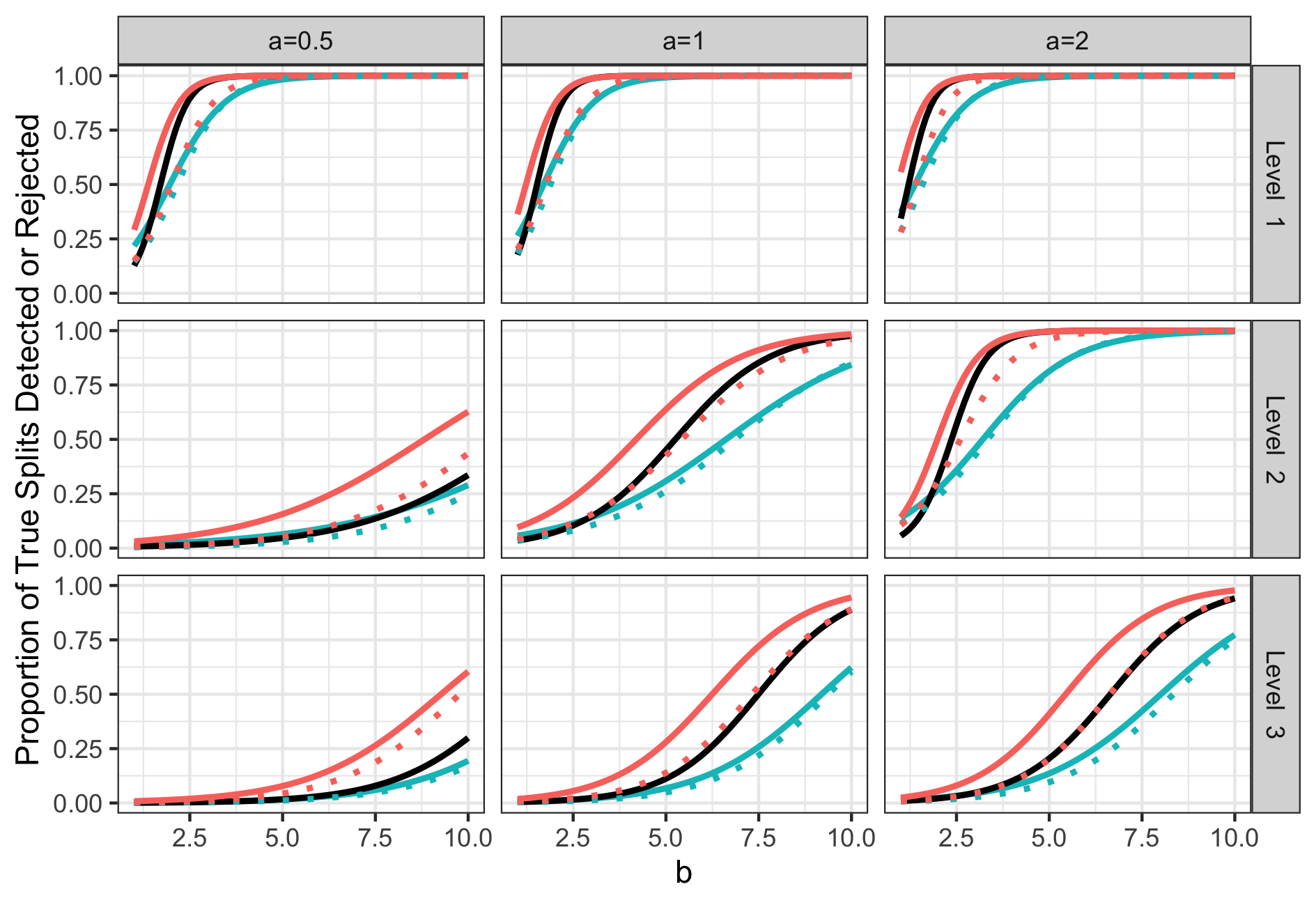
We generate 500 datasets for each , and evaluate the power of selective -tests, sample splitting, and CTree to reject the null hypothesis . As naive -tests do not control the Type 1 error rate (Figure 4), we do not evaluate their power. We consider two aspects of power: the probability that we detect a true split, and the probability that we reject the null hypothesis corresponding to a true split.
A contingency table indicating an observation’s involvement in a given true split and estimated split. The adjusted Rand index is computed using only the shaded cells Estimated Split In left region In right region In neither True Split In left region In right region In neither
Given a true split in Figure 3 and an estimated split, we construct the contingency table in Table 5.4, which indicates whether an observation is on the left-hand side, right-hand side, or not involved in the true split (rows) and the estimated split (columns). To quantify the agreement between the true and estimated splits, we compute the adjusted Rand index [Hubert and Arabie, 1985] associated with the contingency table corresponding to the shaded region in Table 5.4. For each true split, we identify the estimated split for which the adjusted Rand index is largest; if this index exceeds then this true split is “detected”. Given that a true split is detected, the associated null hypothesis is rejected if the corresponding -value is below . Figure 5 displays the proportion of true splits that are detected and rejected by each method.
As sample splitting fits a tree using only half of the data, it detects fewer true splits, and thus rejects the null hypothesis for fewer true splits, than the selective -test.
When is small, the difference in means between sibling regions at level two is small. Because CTree makes a split only if there is strong evidence of association at that level, it tends to build one-level trees, and thus fails to detect many true splits; by contrast, the selective Z-test (based on CART) successfully builds more three-level trees. Thus, when is small, the selective Z-test detects (and rejects) more true differences than CTree between regions at levels two and three.
5.5 Coverage of Confidence Intervals for and
We generate 500 datasets for each to evaluate the coverage of 95% confidence intervals constructed using naive -methods, selective -methods, and sample splitting. CTree is omitted from these comparisons because it does not provide confidence intervals. We say that the interval covers the truth if it contains , where is defined as in (6) (for a particular split) or (14) (for a particular region). Table 5.6 shows the proportion of each type of interval that covers the truth, aggregated across values of and . The selective -intervals attain correct coverage of 95%, while the naive -intervals do not.
It may come as a surprise that sample splitting does not attain correct coverage. Recall that from (6) or (14) is an -vector that contains entries for all observations in both the training set and the test set. Thus, involves the true mean among both training and test set observations in a given region or pair of regions. By contrast, sample splitting attains correct coverage for a different parameter involving the true means of only the test observations that fall within a given region or pair of regions.
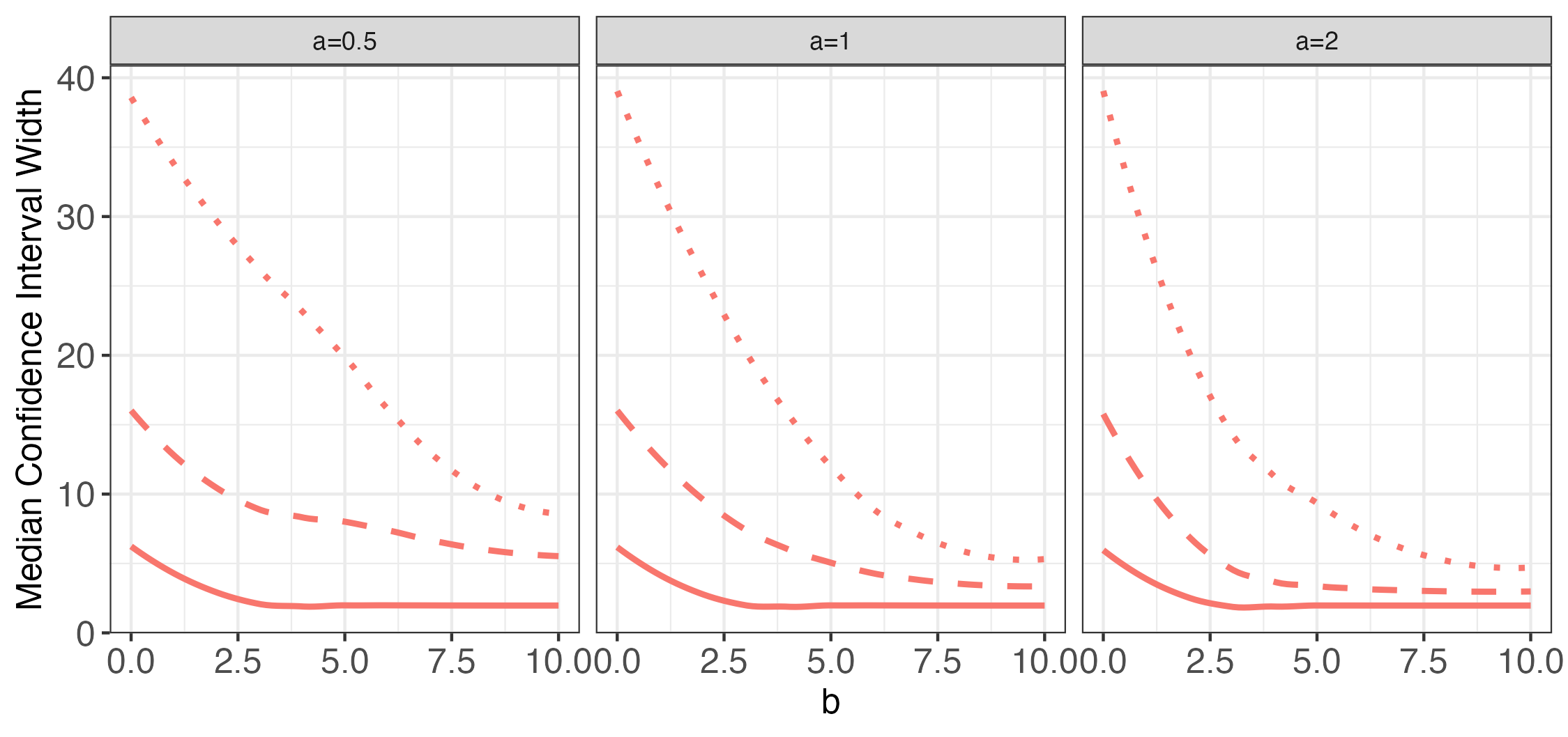
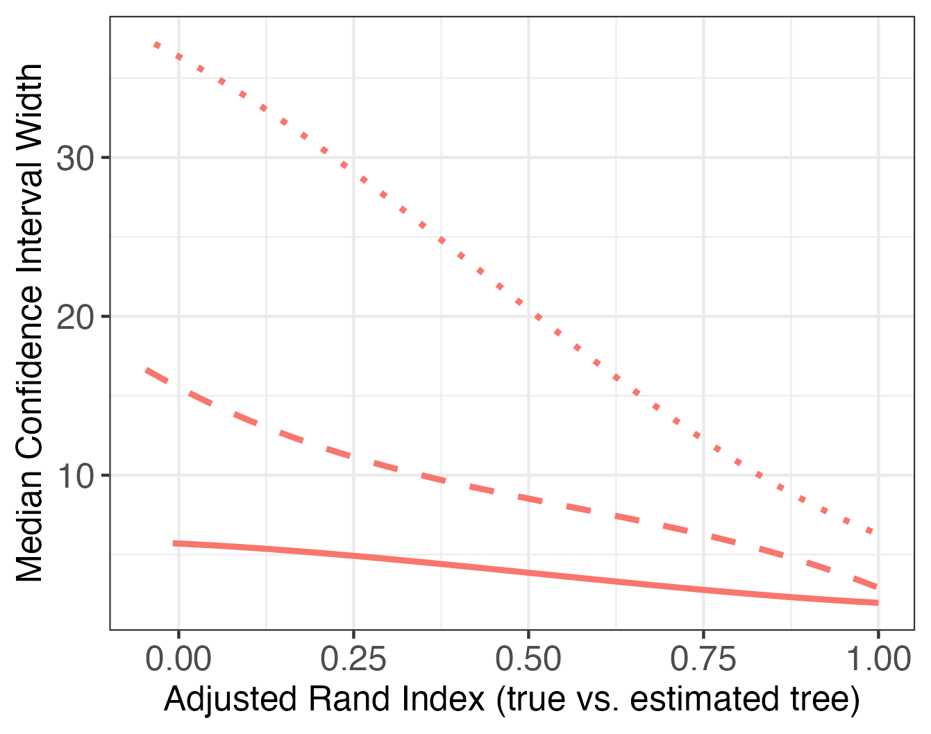
5.6 Width of Confidence Intervals
Figure 6(a) illustrates that our selective -intervals for can be extremely wide when is small, particularly for regions located at deeper levels in the tree. For each tree that we build and for levels 1, 2, and 3, we compute the adjusted Rand Index [Hubert and Arabie, 1985] between the true tree (truncated at the appropriate level) and the estimated tree (truncated at the same level). Figure 6(b) shows that our selective confidence intervals can be extremely wide when this adjusted Rand Index is small, particularly at deeper levels of the tree.
When is small and the adjusted Rand Index is small, the trees built by CART tend to be unstable, in the sense that small perturbations to the data affect the fitted tree. In this setting, the sample statistics fall very close to the boundary of the truncation set. See Kivaranovic and Leeb [2021] for a discussion of why wide confidence intervals can arise in these settings. The great width of our confidence intervals reflects the uncertainty about the mean response within each region due to the instability of the tree-fitting procedure.
Proportion of 95% confidence intervals containing the true parameter, aggregated over all trees fit to the 5,500 datasets generated with Parameter Parameter Level Selective Naive Sample Splitting Selective Naive Sample Splitting 1 0.951 0.889 0.918 0.948 0.834 0.915 2 0.950 0.645 0.921 0.951 0.410 0.917 3 0.951 0.711 0.921 0.950 0.550 0.921
(a) (b)
5.7 Results with Unknown
Thus far, we have assumed that is known. In this section, we compare the following three versions of the selective -methods that plug different values of into the truncated normal CDF when computing p-values and confidence intervals:
- 1.
-
2.
: We plug in , where .
-
3.
Let be the number of terminal regions in . We plug in , where is the predicted value for the th observation given by .
It is straightforward to show that , for any value of . Thus, we expect this estimate to lead to conservative inference. On the other hand, can be made arbitrarily small by making the fitted tree arbitrarily deep, and so we expect inference based on this estimate to be anti-conservative if the fitted CART tree is large.
Figure 7 shows the distribution of p-values from testing with the three versions of the selective -test under the data generating mechanism described in Section 5.1, with . In this setting, holds for all splits in all trees. We see almost no difference between the three versions of the selective -test. In this global null setting, . Furthermore, the empirical bias of is small because the trees we grow are not particularly large; as in the rest of Section 5, we build trees to a maximum depth of 3 and prune with .
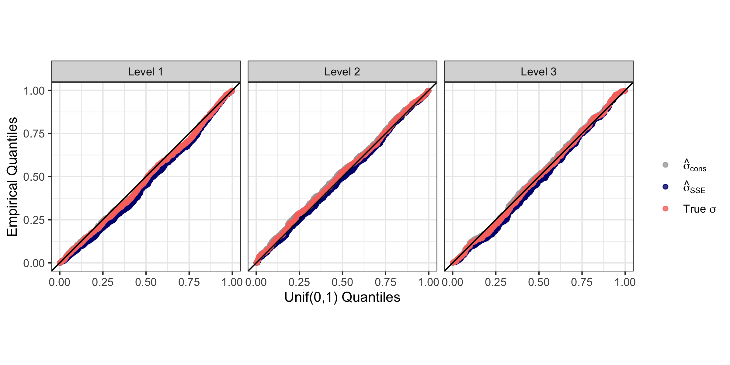
Figure 8 displays the proportion of true splits detected and the proportion of true splits detected and rejected, as defined in Section 5.4, for the three versions of the selective -test when data is generated as in Section 5.4. For simplicity, we only show the setting where . All three methods detect the same proportion of true splits, because they all perform inference on the same CART trees. The proportion of splits detected and rejected is very similar for and because is a very good estimator for in this setting. While performs reasonably when is small, it severely overestimates and thus has low power when is large.
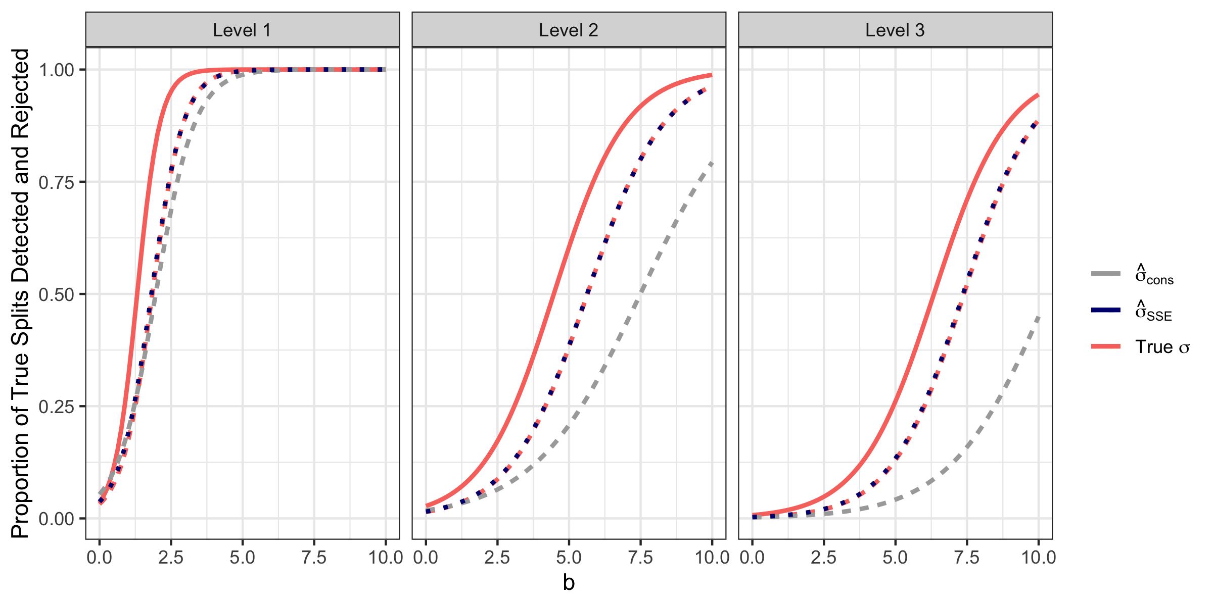
Table 1 displays confidence intervals for and for the three versions of the selective -intervals, where data is generated as in Section 5.5. As expected, leads to slight over-coverage and leads to slight under-coverage.
| Parameter | Parameter | |||||||
|---|---|---|---|---|---|---|---|---|
| Level | ||||||||
| 1 | 0.95 | 0.98 | 0.95 | 0.95 | 0.98 | 0.94 | ||
| 2 | 0.95 | 0.97 | 0.94 | 0.95 | 0.97 | 0.94 | ||
| 3 | 0.95 | 0.96 | 0.94 | 0.95 | 0.96 | 0.94 | ||
In this section, we have seen that when trees are not grown overly large, plugging in leads to approximate selective Type 1 error control, approximately correct selective coverage, and good power. Unfortunately, providing theoretical guarantees for our procedures when using would be quite difficult, as the estimator is anti-conservative and depends on the output of CART. Providing theoretical guarantees for our procedures under is more straightforward, using ideas from Gao et al. [2020], Chen and Witten [2022], and Tibshirani et al. [2018]. However, as shown in Figure 8, selective -tests based on can have very low power. One promising avenue of future work involves providing theoretical guarantees in the regression tree setting for estimators that are less conservative than .
6 An Application to the Box Lunch Study
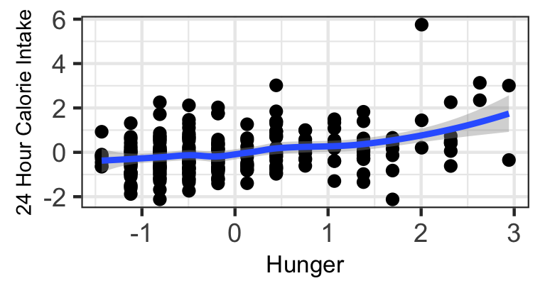
Venkatasubramaniam et al. [2017] compare CART and CTree [Hothorn et al., 2006] within the context of epidemiological studies. They conclude that CTree is preferable to CART because it provides p-values for each split, even though CART has higher predictive accuracy. Since our framework provides p-values for each split in a CART tree, we revisit their analysis of the Box Lunch Study, a clinical trial studying the impact of portion control interventions on 24-hour caloric intake. We consider
identifying subgroups of study participants with baseline differences in 24-hour caloric intake on the basis of scores from an
assessment that quantifies constructs such as hunger, liking, the relative reinforcement of food (rrvfood), and restraint (resteating).
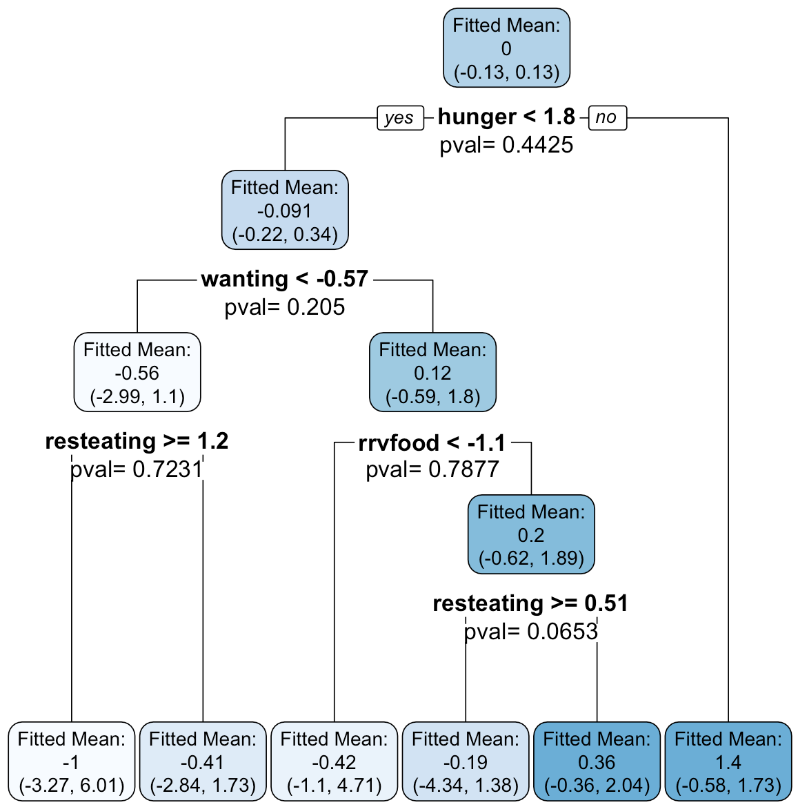
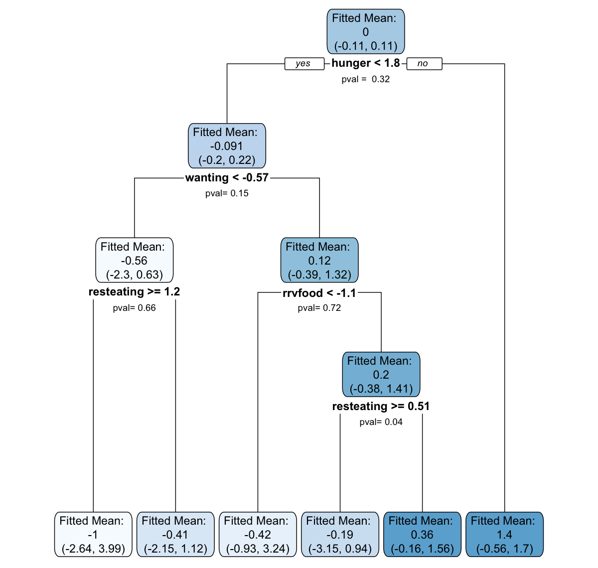
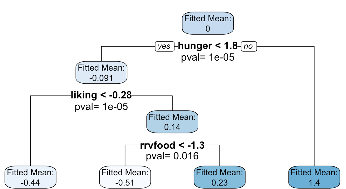
We exactly reproduce the trees presented in Figures 1 and 2 of Venkatasubramaniam et al. [2017] by building a CTree using partykit and a CART tree using rpart on the Box Lunch Study data provided in the R package visTree [Venkatasubramaniam and Wolfson, 2018]. We apply our selective inference framework to compute p-values (8) for each split in CART, and confidence intervals (4.3) for each region. In this section, we use , defined in Section 5.7, to estimate the error variance. The results are shown in Figure 9.
Both CART and CTree choose hunger1.8 as the first split. For this split, our selective -test reports a large p-value of 0.44, while CTree reports a p-value less than 0.001. The conflicting p-values are explained by the difference in null hypotheses. CTree finds strong evidence against the null of no linear association between hunger and caloric intake. By contrast, our selective framework for CART does not find strong evidence for a difference between mean caloric intake of participants with hunger1.8 and those with hunger1.8. We see from the bottom right of Figure 9 that while there is evidence of a linear relationship between hunger and caloric intake, there is less evidence of a difference in means across the particular split hunger1.8. Given that the goal of Venkatasubramaniam et al. [2017] is to “identify population subgroups that are relatively homogeneous with respect to an outcome”, the p-value resulting from our selective framework is more natural than the p-value output by CTree, since the former relates directly to the subgroups formed by the split, whereas the latter does not take into account the location of the split point. In general, the left-hand panel of Figure 9 shows that the subgroups of patients identified by CART are not significantly different from one another. This is an important finding that would be missed without our selective inference framework. Furthermore, unlike CTree, our framework provides confidence intervals for the mean response in each subgroup.
7 Discussion
Our framework relies on the assumption that , with known. In Section 5.7, we showed strong empirical performance when the variance is unknown and is estimated. In this section, we briefly comment on the assumptions of spherical variance and normally distributed data.
It natural to wonder whether the assumption that can be relaxed to the assumption that , with known. Following the work of Lee et al. [2016], the results in Section 3 extend to the setting where if we:
- 1.
-
2.
Replace all instances of the perturbation , defined in Theorem 1, with the perturbation
Unfortunately, the modified perturbation does not satisfy Condition 1 in Section 4.2 when , and so many of the results of Section 4 do not extend to this non-spherical setting. Future work could explore how to efficiently compute the conditioning set in this non-spherical setting.
Furthermore, our framework assumes a normally-distributed response variable. CART is commonly used for classification, survival [Segal, 1988], and treatment effect estimation in causal inference [Athey and Imbens, 2016]. While the idea of conditioning on a selection event to control the selective Type 1 error rate applies regardless of the distribution of the response, our Theorem 1 and Theorem 2, and the resulting computational results, relied on normality of . In the absence of this assumption, exactly characterizing the conditioning set and the distribution of the test statistic requires further investigation.
We show in Appendix G that our selective -tests approximately control the selective Type 1 error when the normality assumption is violated. Tian and Taylor [2017] and Tibshirani et al. [2018] establish conditions under which selective p-values for linear regression (derived under the assumption of normality) will be asymptotically uniformly distributed under non-normality. Thus suggests the possibility of developing asymptotic theory for our proposed selective -tests under violations of normality.
A reviewer pointed out similarities between the problem of testing significance of the first split in the tree and significance testing for a single changepoint, as in Bhattacharya [1994]. Building on this connection may provide an avenue for future work.
A software implementation of the methods in this paper is available in the R package treevalues, at https://github.com/anna-neufeld/treevalues.
Acknowledgements
Daniela Witten and Anna Neufeld were supported by the National Institutes of Health and the Simons Foundation. Lucy Gao was supported by the Natural Sciences and Engineering Research Council of Canada Discovery Grants program.
References
- Athey and Imbens [2016] Susan Athey and Guido Imbens. Recursive partitioning for heterogeneous causal effects. Proceedings of the National Academy of Sciences, 113(27):7353–7360, 2016.
- Bhattacharya [1994] PK Bhattacharya. Some aspects of change-point analysis. Lecture Notes-Monograph Series, pages 28–56, 1994.
- Bourgon [2009] Richard Bourgon. Overview of the intervals package, 2009. R Vignette, URL https://cran.r-project.org/web/packages/intervals/vignettes/intervals_overview.pdf.
- Breiman et al. [1984] Leo Breiman, Jerome Friedman, Charles J Stone, and Richard A Olshen. Classification and regression trees. CRC Press, 1984.
- Chen and Bien [2020] Shuxiao Chen and Jacob Bien. Valid inference corrected for outlier removal. Journal of Computational and Graphical Statistics, 29(2):323–334, 2020.
- Chen and Witten [2022] Yiqun T Chen and Daniela M Witten. Selective inference for k-means clustering. arXiv preprint arXiv:2203.15267, 2022.
- Fithian et al. [2014] William Fithian, Dennis Sun, and Jonathan Taylor. Optimal inference after model selection. arXiv preprint arXiv:1410.2597, 2014.
- Gao et al. [2020] Lucy L Gao, Jacob Bien, and Daniela Witten. Selective inference for hierarchical clustering. arXiv preprint arXiv:2012.02936, 2020.
- Hothorn and Zeileis [2015] Torsten Hothorn and Achim Zeileis. partykit: A modular toolkit for recursive partytioning in R. The Journal of Machine Learning Research, 16(1):3905–3909, 2015.
- Hothorn et al. [2006] Torsten Hothorn, Kurt Hornik, and Achim Zeileis. Unbiased recursive partitioning: A conditional inference framework. Journal of Computational and Graphical Statistics, 15(3):651–674, 2006.
- Hubert and Arabie [1985] Lawrence Hubert and Phipps Arabie. Comparing partitions. Journal of Classification, 2(1):193–218, 1985.
- Hyun et al. [2021] Sangwon Hyun, Kevin Z Lin, Max G’Sell, and Ryan J Tibshirani. Post-selection inference for changepoint detection algorithms with application to copy number variation data. Biometrics, pages 1–13, 2021.
- Jewell et al. [2022] Sean Jewell, Paul Fearnhead, and Daniela Witten. Testing for a change in mean after changepoint detection. Journal of the Royal Statistical Society, Series B, 2022.
- Kivaranovic and Leeb [2021] Danijel Kivaranovic and Hannes Leeb. On the length of post-model-selection confidence intervals conditional on polyhedral constraints. Journal of the American Statistical Association, 116(534):845–857, 2021.
- Lee et al. [2016] Jason D Lee, Dennis L Sun, Yuekai Sun, Jonathan E Taylor, et al. Exact post-selection inference, with application to the lasso. The Annals of Statistics, 44(3):907–927, 2016.
- Liu et al. [2018] Keli Liu, Jelena Markovic, and Robert Tibshirani. More powerful post-selection inference, with application to the lasso. arXiv preprint arXiv:1801.09037, 2018.
- Loh [2014] Wei-Yin Loh. Fifty years of classification and regression trees. International Statistical Review, 82(3):329–348, 2014.
- Loh et al. [2016] Wei-Yin Loh, Haoda Fu, Michael Man, Victoria Champion, and Menggang Yu. Identification of subgroups with differential treatment effects for longitudinal and multiresponse variables. Statistics in medicine, 35(26):4837–4855, 2016.
- Loh et al. [2019] Wei-Yin Loh, Michael Man, and Shuaicheng Wang. Subgroups from regression trees with adjustment for prognostic effects and postselection inference. Statistics in Medicine, 38(4):545–557, 2019.
- Ripley [1996] Brian D Ripley. Pattern recognition and neural networks. Cambridge University Press, 1996.
- Segal [1988] Mark Robert Segal. Regression trees for censored data. Biometrics, 44(1):35–47, 1988.
- Taylor and Tibshirani [2015] Jonathan Taylor and Robert J Tibshirani. Statistical learning and selective inference. Proceedings of the National Academy of Sciences, 112(25):7629–7634, 2015.
- Therneau and Atkinson [2019] Terry Therneau and Beth Atkinson. rpart: Recursive Partitioning and Regression Trees, 2019. R package version 4.1-15, available on CRAN.
- Tian and Taylor [2017] Xiaoying Tian and Jonathan Taylor. Asymptotics of selective inference. Scandinavian Journal of Statistics, 44(2):480–499, 2017.
- Tian and Taylor [2018] Xiaoying Tian and Jonathan Taylor. Selective inference with a randomized response. The Annals of Statistics, 46(2):679–710, 2018.
- Tibshirani et al. [2016] Ryan J Tibshirani, Jonathan Taylor, Richard Lockhart, and Robert Tibshirani. Exact post-selection inference for sequential regression procedures. Journal of the American Statistical Association, 111(514):600–620, 2016.
- Tibshirani et al. [2018] Ryan J Tibshirani, Alessandro Rinaldo, Rob Tibshirani, and Larry Wasserman. Uniform asymptotic inference and the bootstrap after model selection. The Annals of Statistics, 46(3):1255–1287, 2018.
- Venkatasubramaniam and Wolfson [2018] Ashwini Venkatasubramaniam and Julian Wolfson. visTree: Visualization of Subgroups for Decision Trees, 2018. R package version 0.8.1, available on CRAN.
- Venkatasubramaniam et al. [2017] Ashwini Venkatasubramaniam, Julian Wolfson, Nathan Mitchell, Timothy Barnes, Meghan JaKa, and Simone French. Decision trees in epidemiological research. Emerging Themes in Epidemiology, 14(1):11, 2017.
- Wager and Walther [2015] Stefan Wager and Guenther Walther. Adaptive concentration of regression trees, with application to random forests. arXiv preprint arXiv:1503.06388, 2015.
Appendix A Comparison to Loh et al. [2019]
Loh et al. [2016] and Loh et al. [2019] use regression trees to find subgroups of patients with similar treatment effects in clinical trials. They grow trees based on patient characteristics using a different algorithm than CART. Furthermore, they are interested in the mean treatment effect (which is a linear regression coefficient) within each terminal region of the tree, rather than the mean response within each region.
One of the goals of Loh et al. [2019] is to construct valid post-selection confidence intervals for the treatment effect within each terminal node. In this appendix, we show that their approach, when adapted to the setting of this paper, does not yield confidence intervals with nominal coverage.
The basic idea of Loh et al. [2019], instantiated to our setting, is as follows. Suppose that , and define the vector such that , as in (14). We know that the “naive” Z-interval does not achieve nominal coverage, meaning that
| (24) |
This is because the “multiplier” for the naive confidence interval, , is derived under the assumption that the region (or, equivalently, the vector ), is fixed, rather than a function of the data.
Loh et al. [2019] observe that there exists some such that
| (25) |
The value for for a given tree will depend on the number of split covariates , the number of data points , the depth of the tree, and the value of used for tree pruning, among other considerations. If we know how the data was generated, then we can check whether some value satisfies (25) as follows:
-
1.
Draw different simulated datasets from the same distribution (call this ) as the original data. For :
-
(a)
Build a tree using the simulated data , using the same procedure and the same settings as in Step 1, and denote it .
-
(b)
For each terminal region in the tree:
-
i.
Construct a naive -interval for the mean response in the region using .
-
ii.
Check if each interval contains , the true mean for this region .
-
i.
-
(a)
-
2.
Compute the fraction of intervals in 1(b) that contain .
-
3.
If this value is , then we have found the correct value of . If not, then we try a larger or smaller value of .
We test this procedure in a very simple simulation study. We generate data and for and . In this simple setting, the true mean response for every region in every fitted tree is . We carry out the procedure outlined above with . For two values of and for CART trees with 1, 2, and 3 levels, we create 1000 datasets and 1000 trees and report the empirical coverage of the intervals obtained using this ideal method, averaged over all nodes in all trees. The results, shown in Table 2, show that this ideal procedure procedure leads to intervals that achieve nominal coverage.
Unfortunately, this ideal procedure is practically infeasible, as it requires the user to know the true distribution of the data . Thus, in practice, Loh et al. [2019] propose replacing by , the empirical distribution of the original data. This amounts to replacing the simulated datasets in Step 2 with bootstrapped datasets, and checking whether the naive -intervals in Step 1(b) contain rather than .
We can see why this is problematic in a very simple setting where we fit a tree with depth 1. If all observations have mean , then a CART tree fit to a bootstrap sample of the data will nevertheless find regions and such that the sample mean value of within is negative and the sample mean value of within is positive. As and contain many overlapping observations, it is likely that the sample mean value of within is also negative and the sample mean value of within is also positive. In other words, because of the overlap between and , the within-region sample means of are closer to the within-region sample means of than they are to the within-region population means. Thus, when we calibrate to cover the mean values of within various regions, we end up with under-coverage of the true population mean, as shown in Table 2.
We see in Table 2 that our selective inference framework approach enables valid inference in this setting, whereas a bootstrap procedure modeled after Loh et al. [2019] does not.
| Loh (ideal) | Loh (bootstrap) | Selective CIs | ||||
|---|---|---|---|---|---|---|
| p | Tree depth | Coverage | Average | Coverage | Average | Coverage |
| 1 | 0.902 | 0.008 | 0.749 | 0.037 | 0.890 | |
| 2 | 2 | 0.905 | 0.004 | 0.695 | 0.038 | 0.904 |
| 3 | 0.900 | 0.005 | 0.660 | 0.047 | 0.895 | |
| 1 | 0.883 | 0.001 | 0.601 | 0.016 | 0.908 | |
| 20 | 2 | 0.900 | 0.00025 | 0.549 | 0.016 | 0.901 |
| 3 | 0.904 | 0.00015 | 0.543 | 0.022 | 0.905 | |
Appendix B Proofs for Section 3
B.1 Proof of Theorem 1
Let . We start by proving the first statement in Theorem 1:
This is a special case of Proposition 3 from Fithian et al. [2014]. It follows from the definition of in (8) that
Therefore, applying the law of total expectation yields
The second statement of Theorem 1 follows directly from the following result.
Lemma 3.
If , then the random variable has the following conditional distribution:
| (26) |
where is defined in (10) and denotes the distribution truncated to the set .
Proof.
The following holds for any .
where In the fourth line, the condition can be dropped because when , is independent of . Finally, since , (26) holds. ∎
B.2 Proof of Proposition 1
Theorem 6.1 from Lee et al. [2016] says that the truncated normal distribution has monotone likelihood ratio in the mean parameter. This guarantees that and in (13) are unique. Then, for and in (13), (26) in Lemma 3 guarantees that
| (27) |
Finally, we need to prove that (27) implies –selective coverage as defined in (12). Following Proposition 3 from Fithian et al. [2014], let be the random variable and let be its density. Then,
B.3 Proof of Theorem 2
We omit the proof of the first statement of Theorem 2, as it is similar to the proof of the first statement of Theorem 1 in Appendix B.1.
The second statement in Theorem 2 follows directly from the following result.
Lemma 4.
B.4 Proof of Proposition 2
The proof largely follows the proof of Proposition 1. The fact that the truncated normal distribution has monotone likelihood ratio (Theorem 6.1 of Lee et al. 2016) ensures that and defined in (17) are unique, and (28) in Lemma 4 implies that
The rest of the argument is as in the proof of Proposition 1.
Appendix C Proofs for Section 4.1
C.1 Proof of Lemma 1
We first state and prove the following lemma.
Lemma 5.
Proof.
We will now prove Lemma 1.
It follows from Definition 6 that if , then and are siblings in . This establishes the direction.
We will prove the direction by contradiction. Suppose that and are siblings in . Define , and define for . Assume that there exists such that and . We assume that any ties between splits that occur at Step 2 of Algorithm A1 are broken in the same way for and , and so this implies that there exists such that and
| (30) |
C.2 Proof of Lemma 2
Appendix D Proofs for Section 4.2
D.1 Proof of Proposition 3
Recall that and . Recall from (20) that , and that we define .
D.2 Proof of Proposition 4
Given a region , let denote the vector in such that the th element is . Let denote the orthogonal projection matrix onto the vector .
Lemma 6.
For any region , where
| (33) |
Furthermore, the matrix is positive semidefinite.
Proof.
For any region , Thus, from (2),
To see that is positive semidefinite, observe that, for any vector ,
∎
It follows from Lemma 6 that we can express each set from Proposition 3 as
| (34) |
We now use (34) to prove the first statement of Proposition 4.
Lemma 7.
Each set is defined by a quadratic inequality in .
Proposition 3 indicates that to compute from (20), we need to compute the coefficients of the quadratic for each , where , , and .
Lemma 8.
We can compute the coefficients and , defined in Lemma 7, for , , and , in operations.
Proof.
We compute the scalar and the vector in operations once at the start of the algorithm. We also sort each feature in operations per feature. We will now show that for the th level and the th feature, we can compute , and for all values of in operations.
The index appears in (37)–(39) only through , , and through inner products of vectors and with indicator vectors and . For simplicity, we assume that covariate is continuous, and thus the order statistics are unique.
Let be the index corresponding to the smallest value of . Then if observation is in , and is otherwise. Similarly, if observation is in , and is otherwise. Next, let be the index corresponding to the second smallest value of . Then if observation is in , and is equal to otherwise. We compute in the same manner. Each update is done in constant time. Continuing in this manner, computing the full set of quantities and for requires a single forward pass through the sorted values of , which takes operations. The same ideas can be applied to compute , , , and using constant time updates for each value of .
Thus, we can obtain all components of coefficients , and for a fixed and , and for all , in operations. These scalar components can be combined to obtain the coefficients in operations. Therefore, given the sorted features, we compute the coefficients in operations. ∎
Once the coefficients on the right hand side of (D.2) have been computed, we can compute in constant time via the quadratic equation: it is either a single interval or the union of two intervals. Finally, in general we can intersect intervals in operations [Bourgon, 2009]. The final claim of Proposition 4 involves the special case where and .
Lemma 9.
Suppose that from (6) and . (i) If , then for all and , there exist such that and . (ii) If , then for all and , there exist such that and . (iii) We can intersect all sets of the form in operations.
Proof.
This proof relies on the form of given in (D.2). To prove (i), note that when ,
The first equality follows directly from the definition of in (35). To see why the second equality holds, observe that , and without loss of generality assume that . Recall that the th element of is non-zero if and only if , and that the non-zero elements of sum to . Thus, and . Furthermore, the supports of and are non-overlapping, and so . Thus,
The final inequality follows because is positive semidefinite (Lemma 6).
Thus, when , is defined in (D.2) by a quadratic inequality with a non-negative quadratic coefficient. Thus, must be a single interval of the form . Furthermore, since , we know that . Therefore, , and so we conclude . This completes the proof of (i).
To prove (ii), we first prove that when the quadratic equation in defined in (D.2) has a non-positive quadratic coefficient. To see this, note that
| (40) |
The first equality follows from (35). The second follows from the definition of given in (33) and from the fact that because sums up all of the non-zero elements of , which sum to . The third equality follows because lies in ; projecting it onto this span yields itself. Noting that is itself a projection matrix, the fourth equality follows from the idempotence of projection matrices, and the inequality follows from the fact that for any projection matrix . Thus, when , the quadratic that defines has a non-positive quadratic coefficient.
Equality is attained in (40) if and only if . This can only happen if splitting on yields an identical partition of the data to splitting on . If this is the case, then from the definition of in Proposition 3, and so (ii) is satisfied with .
We now proceed to the setting where the inequality in (40) is strict. In this case, (D.2) implies that for and . To complete the proof of (ii), we must argue that and . Recall that the quadratic in (34) has the form . When , , because eliminates the contrast between and , so that the split on provides zero gain. So, when , the quadratic evaluates to , which is non-negative by Lemma 6. Thus, is defined by a downward facing quadratic that is non-negative when , and so the set has the form for .
To prove (iii), observe that (i) implies that , where is the maximum over all of the ’s, and is the minimum over all of the ’s. This can be computed in steps. Furthermore, (ii) implies that , where and are the minimum over all of the ’s and the maximum over all the ’s, respectively. This can be computed in steps. Thus, we can compute in operations. ∎
D.3 Proof of Proposition 5
To prove Proposition 5, we first propose a particular method of constructing an example of . We then show that (21) holds for this particular choice for . We conclude by evaluating the computational cost of computing such an example of , and by arguing that in the special case where , our example is equal to .
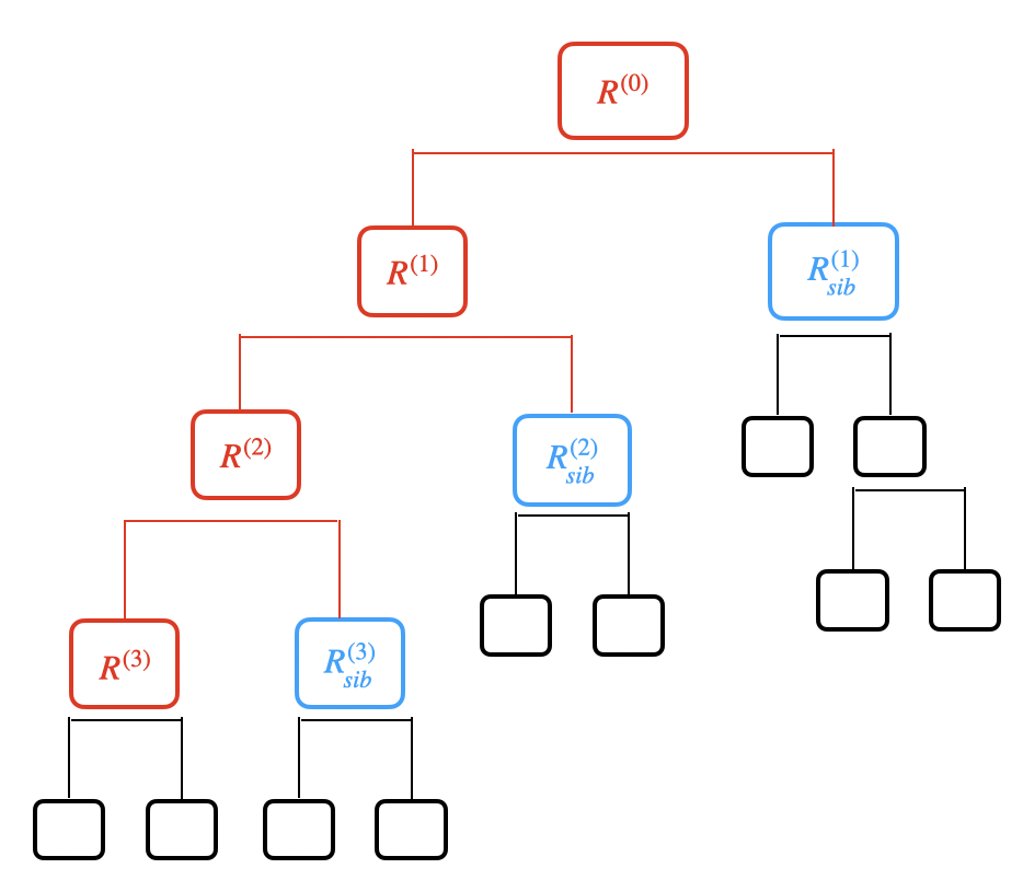
When Algorithm A2 is called with parameters , where is a bottom-up ordering of the nodes in , it computes a sequence of intermediate trees, . We use the notation , for , to denote the th of these intermediate trees. The following lemma helps build up to our proposed example of .
Lemma 10.
Let and . Then . Let be a bottom-up ordering of the regions in such that the last regions in the ordering are . Then .
Proof.
We first prove that , where . The fact that and implies two properties:
-
Property 1: and for by the definition of .
-
Property 2: and for , where . This follows from Property 1 and Definition 1.
Suppose that . Then must belong to one of these three cases, illustrated in Figure 10(a):
-
Case 1: such that . By Property 1, .
-
Case 2: such that . By Property 2, .
-
Case 3: , where either for some , or else . By Properties 1 and 2, . Condition 1 ensures that, for all and for some constants and ,
As constant shifts preserve within-node sums of squared errors, in each of these three scenarios, . Thus, .
Thus, if , then . This completes the argument that . Swapping the roles of and in this argument, we see that . This concludes the proof that .
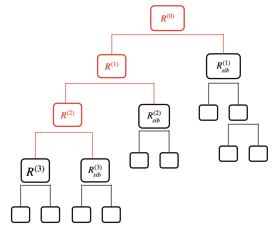
Because , it follows that any bottom-up ordering of the regions in is also a bottom-up ordering for the regions in . We next prove by induction that, if we choose a bottom-up ordering that places the regions in at the end of the ordering, then
| (41) |
for . It follows immediately from Algorithm A2 and the argument above that . Next, suppose that for some ,
| (42) |
and denote this tree with for brevity. We must prove that (41) holds. Let be the th region in and recall the assumption that the last regions in are . Since , this implies that . This means that either for or , meaning that is a black region in Figure 10(b). From Condition 1,
In any of the three cases illustrated in Figure 10, for defined in (3), . Combining this with (42) and Step 2(b) of Algorithm A2 yields (41). This completes the proof by induction.
∎
Since Lemma 10 guarantees that each leads to the same , we will refer to this tree as , will let be the number of regions in this tree, and will let be a bottom-up ordering of these regions that places in the last spots. We will further denote for any as , since Lemma 10 further tells us that this is the same for all . In what follows, we argue that if we let , where appears in the statement of Proposition 5, then (21) holds. In other words, we prove that , which always exists and is well-defined, is a valid example of .
Recall from (18) that . Lemma 10 says that for , we can rewrite as . So we can rewrite as
| (43) |
Furthermore, since (all of which are ancestors of ) are the last nodes in the ordering , we see that if and only if no pruning occurs during the last iterations of Step 2 in Algorithm A2. This means that we can characterize (43) as
| (44) |
Recall that for , is the th region in , and is an ancestor of . We next argue that we can rewrite (44) as
| (45) |
To begin, suppose that . As we are talking about a particular , for we will suppress the dependence of on its arguments and denote it with . The fact that means that
, which ensures that no pruning occurs at step , which in turn ensures that .
Combined with (45), this implies that
, which ensures that no pruning occurs at step , which in turn ensures that . Proceeding in this manner, by tracing through the last iterations of Step 2 of Algorithm A2, we see that satisfies , and so .
Next suppose that (45). Let
As is a minimum, we know that no pruning occurred during steps , and so . This implies that
can be rewritten as
. It then follows from Algorithm A2 that pruning occurs at step , which means that cannot possibly equal . Thus, .
Thus, if and only if .
Finally, Proposition 5 rewrites (45) with the indexing over changed to an indexing over , and plugging in . Therefore, is a valid example of .
To compute , we first select an arbitrary . We then apply Algorithm A1 to grow . We create a bottom-up ordering of the nodes in such that are at the end. Finally, we apply the first iterations of Algorithm A2 with arguments and to obtain . The worst case computational cost of CART (the combined Algorithm A1 and Algorithm A2) is .
In the special case that , we have that because and . In this case, suppose that we carry out the process described in the previous paragraph by selecting . As , it is clear from Algorithm A2 that no pruning occurs during the last iterations of Step 2 in Algorithm A2 applied to arguments and . Therefore, the process from the previous paragraph returns the optimally pruned . Thus, when , we can simply plug in , which has already been built, for in (21).
D.4 Proof of Proposition 6
We first show that we can express
| (46) |
as the solution set of a quadratic inequality in for , where was defined in (3). Because only the numerator of depends on , it will be useful to introduce the following concise notation:
| (47) |
We begin with the following lemma.
Lemma 11.
Suppose that region in has children and . Then, , where is defined in (2).
Proof.
The result follows from adding and subtracting and in (47) and noting that . ∎
Recall that and that . Lemma 12 follows from Lemma 11 and the fact that, due to the form of the vector , there are many regions for which does not depend on .
Lemma 12.
For any , we can decompose as
where is the sibling of in .
Proof.
We can now write (46) as
| (49) |
where the functions and were defined in (35) in Appendix D.2, and where
is a constant that does not depend on . The first equality simply applies the definitions of and . The second equality follows from Lemma 12 and moving terms that do not depend on to the right-hand-side. The third equality follows from plugging in notation from Appendix D.2 and defining the constant for convenience. Thus, (46) is quadratic inequality in . We now just need to argue that its coefficients can be obtained efficiently.
We need to compute the coefficients in (49) for . The quantities , , and for were already computed while computing . To get the coefficients for the left hand side of (49) for each , we simply need to compute partial sums of these quantities, which takes operations. As we are assuming that we have access to , computing requires operations. Therefore, computing takes operations. By storing partial sums during the computation of , we can subsequently obtain for in constant time.
We have now seen that we can obtain the coefficients needed to express (46) as a quadratic function of for in total operations. Once we have these quantities, we can compute each set of the form (46) in constant time using the quadratic equation.
It remains to compute
| (50) |
Recall from Proposition 3 that is the intersection of quadratic sets. Thus, in the worst case, has disjoint components, and so this final intersection involves components. Thus, we can compute in operations [Bourgon, 2009].
The following lemma explains why, similar to Proposition 4, computation time can be reduced in the special case where and .
Lemma 13.
When , the
set
has the form , where . Therefore, we can compute as
in operations. Furthermore, we can compute (50) in constant time.
Proof.
Thus, when and , we can rewrite (49) with all of the terms corresponding to for moved into the constant on the right-hand-side. This lets us rewrite (49) as where is an updated constant that does not depend on .
To prove that has the form for , first recall from Lemma 6 that is a quadratic function of . It then suffices to show that this quadratic has a non-negative second derivative and achieves its minimum when . The second derivative of this quadratic is , which is non-negative by Lemma 6. From Lemma 6, is non-negative. It equals when , because when then .
Intersecting sets of the form for only takes operations, because we simply need to identify the minimum and maximum . Finally, Lemma 9 ensures that has at most two disjoint intervals, and so the final intersection with takes only operations. ∎
D.5 Proof of Proposition 7
Appendix E Proofs for Section 4.3
E.1 Proof of Proposition 8
As stated in Proposition 8, let
First, we will show that the test based on controls the selective Type 1 error rate, defined in (4); this is a special case of Proposition 3 from Fithian et al. [2014].
Define , , and
. Recall that the test
of based on controls the selective Type 1 error rate if, for all , . By construction,
Let . An argument similar to that of Lemma 2 indicates that . The law of total expectation then yields
Thus, the test based on controls the selective Type 1 error rate. We omit the proof that can be computed as
for , as the proof is similar to the proof of Theorem 1.
Appendix F Effect of Using the Computationally Efficient Alternative in Section 4.3
In this section, we investigate the effect of using from (22) rather than from (15) on power. We also investigate the effect of using (4.3) rather than (17) on the width of confidence intervals for .
We generate data as described in Section 5.1, but for simplicity we restrict our attention to the case where (corresponding to the center panel of Figure 3).
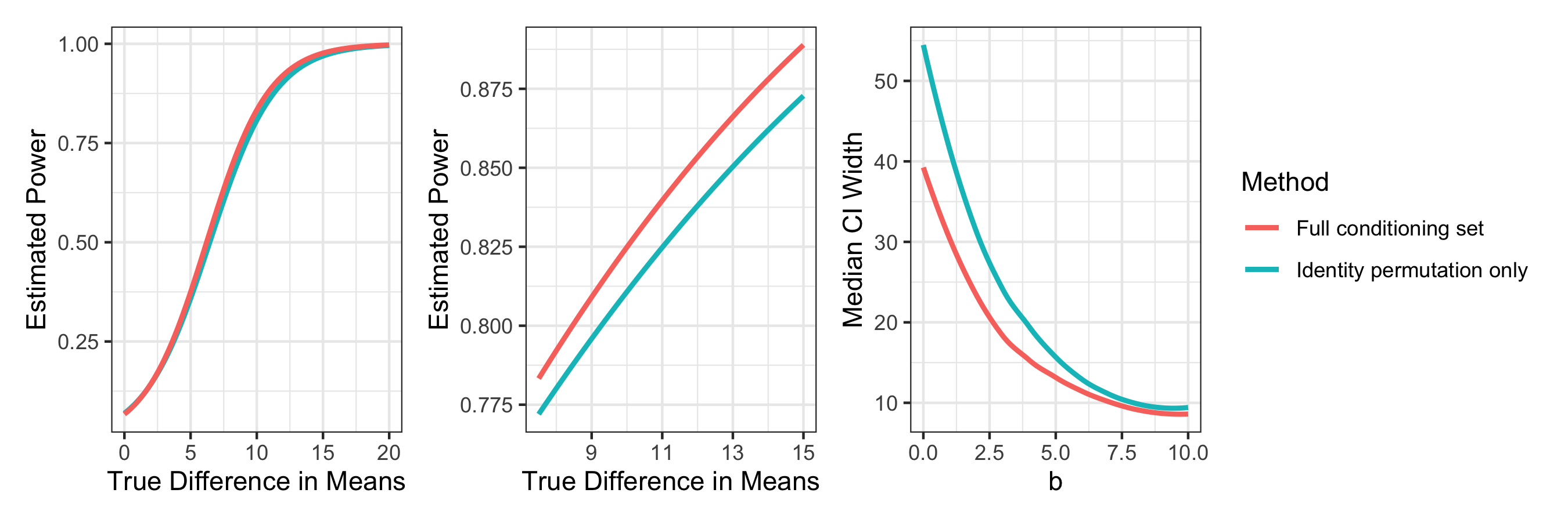
For each tree that we build, we consider (a) testing and (b) constructing a confidence interval for , for each region appearing at the third level of the tree. For each test, we compare the test that uses the full conditioning set (i.e. that uses from (15)) to the test that uses the identity permutation only (i.e. that uses from (22)). For each interval, we compare the method that uses the full conditioning set (i.e. (17)) to the method that uses the identity permutation only (i.e. (4.3)). The results are displayed in Figure 11.
The left panel of Figure 11 shows that the power loss resulting from using (22) instead of (15) is negligible. In fact, we need to zoom in on the left panel, as shown in the center panel, to see any separation between the power curves. We see in the center panel that power is lower when (22) is used, though we emphasize that the differences in power are extremely small.
We see in the right panel of Figure 11 that the computationally efficient conditioning set has a more noticeable impact on the median width of our confidence intervals. As expected, the confidence intervals are narrower when we use the full conditioning set (i.e. (17)). However, this difference is most noticeable when is small. When is small, in which case the confidence intervals are wide even when the full conditioning set is used. Thus, the amount of precision lost overall by constructing confidence intervals using the identity permutation only (i.e. (4.3)) is not of practical importance.
Based on these results, we recommend using the identity permutation in practice, because it is the most computationally efficient choice and does not meaningfully reduce power or precision compared to the full conditioning set.
Appendix G Robustness to Non-Normality
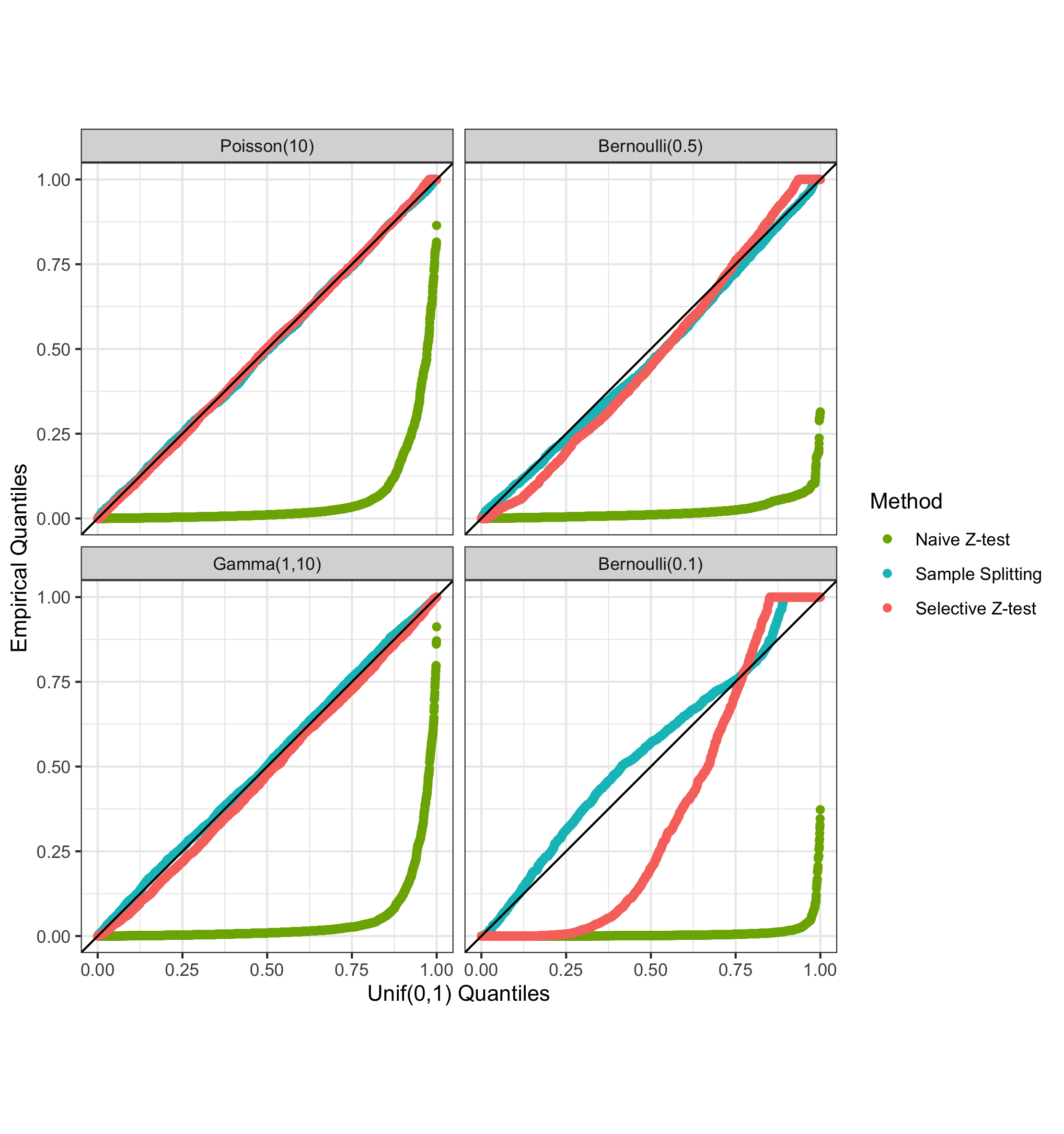
In this section, we explore the performance of the selective -test under a global null when the normality assumption on is violated. For four choices of cumulative distribution function , we generate such that all observations have the same expected value. We set , and we grow trees to a maximum depth of . We plug in as an estimate of , as it does not make sense to assume known variance for distributions with a mean-variance relationship. Figure 12 displays quantile-quantile plots of the p-values for testing , using the test in (8).
Figure 12 shows that despite the fact that our proposed selective inference framework was derived under a normality assumption, it yields approximately uniformly distributed p-values for Poisson(10), Bernoulli(0.5), and Gamma(1,10) data. We suspect that this is because is approximately independent of for these distributions (see the proof of Theorem 1 in Appendix B). In the case of Bernoulli(0.1) data, which represents a particularly extreme violation of the normality assumption, the p-values from our selective -test are not uniformly distributed. As mentioned in Section 7, future work could involve characterizing conditions for under which our selective -tests will approximately control the selective Type 1 error.
Appendix H Alternate Box Lunch Study Analysis
Figure 13 is the same as the left panel of Figure 9, but the selective -inference is carried out with , from Section 5.7, rather than . The takeaways presented in Section 6 do not change.