Non-Autoregressive Electron Redistribution Modeling for Reaction Prediction

Abstract

Reliably predicting the products of chemical reactions presents a fundamental challenge in synthetic chemistry. Existing machine learning approaches typically produce a reaction product by sequentially forming its subparts or intermediate molecules. Such autoregressive methods, however, not only require a pre-defined order for the incremental construction but preclude the use of parallel decoding for efficient computation. To address these issues, we devise a non-autoregressive learning paradigm that predicts reaction in one shot. Leveraging the fact that chemical reactions can be described as a redistribution of electrons in molecules, we formulate a reaction as an arbitrary electron flow and predict it with a novel multi-pointer decoding network. Experiments on the USPTO-MIT dataset show that, our approach has established a new state-of-the-art top-1 accuracy and achieves at least 27 times inference speedup over the state-of-the-art methods. Also, our predictions are easier for chemists to interpret owing to predicting the electron flows.

1 Introduction

Reaction prediction (Corey & Wipke, 1969), which aims to predict the resulting chemical outcomes from given reactants and reagents, is a fundamental problem in computational chemistry. Reliably predicting such outcomes enables chemists to analyze the feasibility of chemical reactions and design optimal synthesis routes for target molecules, which is of crucial importance for synthesis planning, drug discovery, and material invention. Nevertheless, reaction prediction has remained a foundational challenge owing to the fact that a typical reaction may involve nearly 100 atoms (Jin et al., 2017), which makes fully exploring all possible transformations intractable.

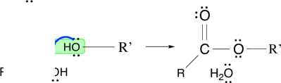
Figure 1: Illustrationof the electron movements in a reaction, where lines represent single covalent bonds (each comprising 2 shared electrons) and a pair of dots representing a lone pair. Each pair of curly arrows show the movement of one electron pair, which results in the bond broken (red curly arrow) and bond formed (blue curly arrow) in the reaction. Such electron redistribution yields the formation and breaking of chemical bonds that change the reactant (left) into product (right). Our approach here aims to model all the movements of electron pairs (i.e., curly arrays) in one shot.

Recently, profound successes have been achieved by applying machine learning to cope with the aforementioned challenge in reaction prediction (Jin et al., 2017; Struble et al., 2020; Shi et al., 2020). For example, (Schwaller et al., 2018, 2019) formulate reaction prediction as a problem of sequence translation by representing molecules as SMILES strings, and Transformer based architecture is used for the translation. More advanced methods (Coley et al., 2019; Do et al., 2019; Sacha et al., 2020) represent molecules as graphs and formulate reaction prediction as iterative graph transformation process. Generally, these methods generate subparts or intermediate molecules of a reaction product in a sequential fashion, through leveraging successive decoding steps.

Despite their dramatic successes, these state-of-the-art end-to-end methods have a major shortcoming, thus hindering their wider applications. That is, these strategies embrace an autoregressive decoding procedure, which produces reaction subparts or intermediate molecule graphs sequentially, each conditioning on previously generated ones. Although autoregressive models can model the dependency between the sequential subparts, there is no unambiguous principle way of linearizing the sequence of steps for constructing a molecular graph, and one failed step in such successive procedure could invalidate the entire synthesis outcomes. Furthermore, such iterative generations hinder parallel decoding for efficient computation.

To cope with the aforementioned limitations, we propose a novel framework for reaction prediction, which predicts reaction outcomes in one shot. We leverage the fact that chemical reactions can be described as a redistribution of electrons in molecules. As illustrated in Figure 2, such electron movement results in the formation and breaking of chemical bonds that convert the reactants into product molecules (Herges, 2015). We here aim to model the simultaneous electron flows in reactants, as such predicting the reaction product is a byproduct of capturing the electron rearrangement in the reactants. In a nutshell, we first formulate an edge in a molecular graph as a pair of shared electrons (i.e., a covalent bond) and bond transformations as electron flows. We then propose a novel electron flow principle to describe arbitrary and parallel electron flows in molecules. We further implement this principle based on the conditional variational autoencoder framework (Sohn et al., 2015) with a novel multi-pointer decoding network to model the incoming and outgoing electron movement probabilities for each atom. This results in modeling arbitrary, non-linear electron flows and simultaneous graph transformations for reaction prediction, hence forming reaction products in one shot. Also, our method possesses beneficial interpretability through showing how the reactants react via the reactivities of electrons. We refer to this model as Non-autoregressive Electron Redistribution Framework (NERF).

We evaluate our model using the benchmarking USPTO-MIT dataset. Our empirical studies show that our approach has established a new state-of-the-art top-1 accuracy. Moreover, our method achieves at least 27 times faster for inference over the state-of-the-art approaches. Our experiments also indicate that the latent variables introduced in our method enable the generation of diverse multi-modal outputs, resulting in top-k accuracy comparable to its autoregressive counterparts. We also demonstrate that due to the prediction of electron flows, our reaction predictions are easier for chemists to interpret.

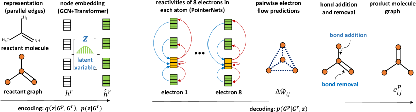
Figure 2: Framework of NERF. The left-bottom depicts the parallel edges in our graph representation $G^{r}$. Encoder is on the left: the node embeddings are generated by a conditional variational auto-encoder CVAE (Sohn et al., 2015). Decoder is on the right: the node embeddings leverage a set of directional PointerNets (Vinyals et al., 2015) to use attention weights to estimate the flow of electron pairs between all the atom pairs in the reaction simultaneously. These electron flows thus reflect the changes of edges and then can be converted into the addition and removal of edges in the reactant molecule to form the product molecule $G^{p}$ (right).

2 Related Work

Data-driven reaction prediction approaches have historically relied on reaction templates, which define sub-graph matching rules for similar organic reactions. Products are generated by first mapping reactants to a set of templates and then applying the pre-defined transformations encoded in the selected templates (Segler & Waller, 2017a, b; Wei et al., 2016), optionally followed by a re-ranking step (Coley et al., 2017). Despite their successful application to synthesis planning, these methods suffer from poor generalization on unseen molecular structures owing to the use of rigidly-defined templates to describe how different chemical substructures may react.

To overcome the limitation of template-based approaches, various template-free methods (Jin et al., 2017; Kayala & Baldi, 2011; Bradshaw et al., 2018; Jin et al., 2017; Coley et al., 2019; Schwaller et al., 2018, 2019; Qian et al., 2020) have recently been introduced. For example, two-stage learning methods have been introduced to achieve promising results (Jin et al., 2017; Qian et al., 2020). One downside of these approaches is that they involve multi-stage learning and cannot be optimized end-to-end. To this end, most state-of-the-art strategies typically embrace an end-to-end, template-free learning paradigm. For example, Schwaller et al. (2018, 2019) leverage a sequence-to-sequence framework to translate SMILES (Weininger, 1988) representations of reactant graphs to those of product graphs. (Bradshaw et al., 2018; Do et al., 2019; Sacha et al., 2020) formulated reaction prediction as a sequence of graph transformations on molecule graph. Such autoregressive methods, however, not only require a pre-defined order for the incremental construction but also hinder parallel decoding for efficient computation. Our strategy overcomes these challenges by embracing a non-autoregressive learning paradigm to generate reaction products in one shot, enabling end-to-end training with parallel decoding for efficient computation.

To the best of our knowledge, our approach is the first attempt to modeling electron flows for non-autoregressive chemical reaction prediction. The only work we are aware of on predicting molecule electron flow is  (Bradshaw et al., 2018). Nevertheless, their approach is limited to a subclass of chemical reactions with “linear” electron flows in an autoregressive format. In contrast, our strategy predicts electron redistribution in one shot. It embraces an arbitrary electron flow principle to capture the parallel electron movement, thus the simultaneous bond making and breaking, in reactant molecules.

3 The Non-Autoregressive Electron Redistribution Framework

In this paper, we formulate the chemical reaction prediction task as a simultaneous electron redistribution problem. We solve this problem by predicting electron flows around each atom in parallel with a conditional variational autoencoder. Specifically, we first employ a graph neural network to encode the reactant graphs, where multiple covalent bonds between atom pairs are represented by parallel binary edges –each depicts two electrons that are shared between the atom pair. In the decoder, the goal is to model the incoming and outgoing electron movement probabilities for each atom (i.e., graph node) in the reactants. Finally, the electron reactivities of the reactants are converted into the addition and removal of edges in the reactant graphs, forming the reaction products. The proposed framework is depicted in Figure 2, and will be discussed in detail next.

3.1 Notation and Problem Formulation

Molecule Graph with Parallel Edges We represent a set of organic molecules as an undirected graph $G=(V,E,f)$, where $V$ and $E$ denote the set of heavy atoms (excluding hydrogen) and bonds, respectively. Each node $v_{i}\in V$ is associated with a fixed-length feature vector ${f_{i}}$, each dimension of which corresponds to a certain property of the atom $v_{i}$ such as atom type or formal electric charge. Unlike previous work where different bond orders are represented by one edge with different features or labels, our method treats different bonds as multiple parallel binary edges, e.g., a double bond is represented as two parallel binary edges (see far left of Figure 2).

Chemical Reaction as Electron Redistribution In this paper, a chemical reaction is described as a pair of molecular graphs $(G^{r},G^{p})$, where $G^{r}=(V,E^{r},f^{r})$ is the set of reactants and $G^{p}=(V,E^{p},f^{p})$ the products we aim to predict. Note that, these two share the same set of nodes $V$. From the chemistry perspective, chemical reactions can be defined as a redistribution of electrons in molecules (Herges, 1994a). In other words, the forming of $E^{p}$ can be described as the rearrangement of electrons in $E^{r}$, which reflects the addition or removal of edges in $E^{r}$ and hence the forming of the products $E^{p}$.

Edge Change as Electron Flow in Molecule From a chemistry perspective, each covalent single bond in organic (carbon-based) molecules represents two electrons that are shared between the atom pair that the bond connects. See illustration in Figure 2. In this paper, we denote $e_{ij}$ ($\geq 0$ and $\in E$) as the number of binary edges (i.e., shared electron pairs) between nodes $v_{i}$ and $v_{j}$, ($v_{i}\in V,v_{j}\in V$), i.e. the number of electrons of atom $i$ that are shared with atom $j$. To this end, we allow self-loops in $G$ and let $e_{ii}$ denote the number of lone pairs in atom $i$ (illustrated as a dot pair around an atom in Figure 2), namely valence electrons that are not shared with other atoms.

From this perspective, an edge change in a molecule is caused by a valence electron’s reactivity. It can form a new bond by sharing with another atom (or form a lone pair through coupling with a sibling atom of its own), or break an existing bond by withdrawing the sharing. Also, based on a chemical rule of thumb known as the Octet Rule, valence electrons that are active in reactions and form bonds is typically no larger than 8. This motivates our aim of modeling the incoming and outgoing electron movement probabilities of each of the 8 valence electrons in each atom during reaction. Consequently, such electron flows reflect the change of edge number before and after the reaction for each atom pair ($i$, $j$), ($v_{i},v_{j}\in V$), namely

$$\Delta e_{ij}=e_{ij}^{p}-e_{ij}^{r}.$$ (1)

In other words, through capturing the reactivity probabilities of the 8 valence electrons in each atom, we can approximating $\Delta e_{ij}$ directly. By doing this, our method can simultaneously access all the edge changes in the reactant molecule, thus produce the reaction products in one shot. Such non-autoreggressive nature distinguishes our strategy from previous work in  (Bradshaw et al., 2018), which can only handle a subclass of chemical reactions that have linear electron flows only.

3.2 The Conditional Variational AutoEncoder Framework

Our goal is to model the probability of product graphs $G^{p}$ conditioning on the reactant graphs $G^{r}$, i.e., $P(G^{p}|G^{r})$. To model the uncertainty of reaction, we introduce a latent variable $z$ and base the whole model on the conditional variational auto-encoder framework (Sohn et al., 2015). For training, we aim to maximize the log-likelihood of each training example, i.e., $\log P(G^{p}|G^{r})$. In practice, it is usually computational intractable to maximize the likelihood $\log P(G^{p}|G^{r})$, and a common approach is to maximize an evidence-lower bound (ELBO) of the log-likelihood as below:

$$\log p(G^{p}|G^{r})\geq{\mathrm{E}}_{q(z|G^{p},G^{r})}[\log p(G^{p}|G^{r},z)]-$$ (2)

$$KL(q(z|G^{p},G^{r})||p(z|G^{r})),$$

where $q(z|G^{p},G^{r})$ is an encoder which defines the variational distribution of the true posterior distribution $p(z|G^{p},G^{r})$, $p(z|G^{r})$ is the prior distribution of the latent variable $z$, and $p(G^{p}|G^{r},z)$ is the decoder. To optimize the lower-bound, we can use the reparametrization trick introduced in the variational auto-encoder (Kingma & Welling, 2013). Next, we will introduce our encoder and decoder respectively.

3.2.1 Encoder

As each reactant is represented as a graph, a natural choice is to encode the atoms of the whole reactants with graph neural networks (Schlichtkrull et al., 2018; Rong et al., 2020), which have been widely studied to learn representations of different kinds of graphs. Let $k$ $\in\mathbb{N}$ be the embedding dimension and $h^{r(l)}_{i}\in\mathbb{R}^{k\times 1}$ the node embeddings of the $i^{th}$ atom at the $l^{th}$ layer computed by the GCN $(h^{r(0)}_{i}=f_{i})$.

At the $l^{th}$ layer, each node $i$ first aggregates the messages from its neighboring nodes, namely $n\in\mathcal{N}_{i}$:

$$m_{i}^{r(l)}=\text{RELU}(W^{(l)}\cdot\text{SUM}\{h_{u}^{r(l-1)}|u\in\mathcal{N}_{i}\}),$$ (3)

where $W^{(l)}\in\mathbb{R}^{k\times k}$ is the trainable weight matrix. The aggregated messages are further combined with the node representation itself by simply taking the summation, yielding a new node representation:

$$h_{i}^{r(l)}=m_{i}^{r(l)}+h_{i}^{r(l-1)}.$$ (4)

As graph convolutional networks only capture the local dependency between atoms, to further model the long-range dependency between atoms, we further apply a Transformer Encoder (Vaswani et al., 2017) on top of the atom representations learned by GCNs, similar to (Rong et al., 2020):

$$h^{r}=\text{Transformer-Encoder}(h^{r(L)}),$$ (5)

where $h^{r(L)}$ are the atom representations in the final layer of the GCN, and $h^{r}$ are the final atom representations of reactants. Similarly, we encode the product graphs with the same neural encoder, obtaining the atom embeddings $h^{p}$ for each atom in $G^{p}$.

Once we have the representations for the reactant and product graphs $h^{r}$ and $h^{p}$, we then use them to define our variational distribution $q(z|G^{p},G^{r})$. Specifically, we first pass the $h^{r}$ and $h^{p}$ through a Transformer-Decoder to compute the cross attention between $h^{r}$ and $h^{p}$. This Transformer-Decoder takes $h^{p}$ as the input sequence of the first decoder layer and $h^{r}$ as the last output sequence of the encoder. Essentially, the atom representations of product graphs $h^{p}$ are treated as memory, and the atom representations of reactants $h^{r}$ are treated as queries, which are updated by attending to $h^{p}$. After that, a mean pooling is further applied to all the atom representations of the reactants, yielding a global representation $h^{z}$ of the reaction:

$$h^{z}=\text{MEAN(Transformer-Decoder}(h^{r},h^{p})).$$ (6)

Next, a fully connected layer with ReLU activation is further applied to $h^{z}$ to define the mean and variance of the latent variable:

$$\mu=W_{\mu}\text{ReLU}(h^{z})+b_{\mu},$$ (7)

$$\text{log}\sigma=W_{\sigma}\text{ReLU}(h^{z})+b_{\sigma}.$$

where $W_{\mu},W_{\sigma}\in\mathbb{R}^{k\times k}$ and $b_{\mu},b_{\sigma}\in\mathbb{R}^{k\times 1}$ are trainable parameters. Therefore, the variational distribution is defined as $q(z|G^{p},G^{r})=\text{Normal}(\mu,\sigma)$. For the prior distribution $p(z|G^{r})$, we simply assume it is a simple standard Gaussian distribution, which does not depend on $G^{r}$.

3.2.2 Decoder

Next, we introduce how to decode the product graph $G^{p}$ based on the latent variable $z$ and the reactant graphs $G^{r}$, i.e., $p(G^{p}|G^{r},z)$. As introduced previously, since the atoms are exactly the same between $G^{r}$ and $G^{p}$, we need to generate the edge difference between the two sets of graphs. We first generate a new set of atom representations for the reactant graphs (denoted as $\hat{h}^{r}$) by taking the summation of each atom representation $h_{i}^{r}$ and the latent variable $z$, followed by a global transformation through a Transformer encoder layer:

$$\hat{h}^{r}_{i}=h^{r}_{i}+z,$$ (8)

$$\hat{h}^{r}=\text{Transformer-Encoder}(\hat{h}^{r}).$$ (9)

Next, these embeddings are then used to generate the edge numbers $e_{ij}^{p}$ for each atom pair ($i$, $j$) in the products. Recall from Section 3.1 that, in order to predict the product graphs, we simply need to model each atom’s electrons activities. According to the Octet Rule as discussed in  3.1, the number of active valence electrons in an atom is typically at most 8, and the reactivity of each electron includes either forming a new bond or breaking an existing bond with another atom (including the atom itself). We here attain this goal by modeling the bond formation and breaking probabilities associating to each electron in each atom using a set of PointerNets (Vinyals et al., 2015).

PointerNet is proposed for selecting an item from a set of items using attention mechanism. In our setting, for each electron of an atom $i$ in reactants $G^{r}$, PointerNet can compute the attentions between atom $i$ and all the atoms in $G^{r}$ (including $i$). The attentions are calculated through a softmax function, thus each of those attention weights can be interpreted as a probability. That is, through the attention weights, a PointerNet provides us the probabilities of atom $i$ initiating an electron flow with all the atoms in the graph.

Consequently, for each electron $d$, we deploy two PointNets: one capturing its probability (denoted $w^{+d}$) of bond formation and another the probability (denoted $w^{-d}$) of bond breaking. We denote these two types of PointerNet as BondFormation and BondBeaking PointerNets, respectively. That is, in total our model has 8 BondFormation PointerNets and 8 BondBeaking PointerNets, and all the 16 PointerNets are shared among all the atoms in the reactants. Formally, give a set of nodes $\hat{h}^{r}$ in the reactants $G^{r}$, a PointerNet can compute an attention weight to reflect the probability of an electron flow from atom $i$ to any atom $j$ in $G^{r}$:

$$w_{ij}^{(+d)}=\text{PointerNet}_{d}^{+}(\hat{h}^{r},i,j),d\in{1,2,\cdots,8}$$ (10)

$$w_{ij}^{(-d)}=\text{PointerNet}_{d}^{-}(\hat{h}^{r},i,j),d\in{1,2,\cdots,8}$$ (11)

where $w_{ij}^{(+d)},w_{ij}^{(-d)}\in[0,1]$.

With the attentions computed by the 16 PointerNets, the overall electron reactivity for an atom pair ($i$, $j$) then can be approximated by calculating the difference between the summation of the 8 BondFormation attentions and that of the 8 BondBreaking attentions:

$$\Delta\tilde{w}_{ij}=\sum_{d=1}^{8}w^{(+d)}_{ij}-\sum_{d=1}^{8}w^{(-d)}_{ij}.$$ (12)

Here, the first and second summations represent the additions and the removals of edges, respectively. Doing so, $\Delta\tilde{w}_{ij}$ thus reflects the change of edge number between the atom pair ($i$, $j$). Next, we then add it to the existing number of edges, i.e., $e^{r}_{ij}$, resulting in the new edge number $\hat{e}_{ij}$ between the atom pair ($i$,$j$):

$$\hat{e}_{ij}=e^{r}_{ij}+\Delta\tilde{w}_{ij}.$$ (13)

Finally, we define our likelihood function as:

$$\log p(G^{p}|G^{r},z) =\sum_{(i,j)\in E^{p}}\log p(e_{ij}^{p}|G^{r},z)$$ (14)

$$\propto-\sum_{(i,j)\in E^{p}}(e_{ij}^{p}-\hat{e}_{ij})^{2}.$$

Generation In practice, given a set of reactant graphs $G^{r}$, to generate the product graphs, $\hat{e}_{ij}$ is rounded to the closest integer to obtain the edge number between the atom pair, namely $e^{p}_{ij}$ :

$$e_{ij}^{p}=\text{round}(\text{min}(\hat{e}_{ij},\hat{e}_{ji})).$$ (15)

Doing so, we then have the resulting modified graph $G^{p}$. During evaluation, a reaction is correctly predicted if the ground truth product is a subgraph of our prediction $G^{p}$ (more detailed illustration will be presented in Figure 5 in the Experiment section).

3.3 Atom Feature Construction and Prediction

We assign each graph node (i.e., atom) with a unique identifier as its positional embedding (You et al., 2019). This ensures that atoms in different chemical environments have distinct node representations. The input features of atoms include atom type, charge, aromaticity, segment embedding and positional embedding. There is no edge feature in our model.

Our proposed NERF framework can easily incorporate domain knowledge owing to the fact that each atom has its own embedding $h^{r}$. In addition to predicting the edge changes in the reactants, our model can naturally leverage the atom embedding $h^{r}$ to predict an atom’s other properties such as its electron charges, aromatic property and chirality.

To this end, we pass the atom embedding $h^{r}_{i}$ through a MLP layer to generate the predicted probabilities of this atom’s aromatic property. Such prediction thus can help us to recover the aromatic bonds, which are typically described as alternating single and double bonds, in the resulting product graphs.

4 Experimental Studies

Table 1: Top-k accuracy on USPTO-MIT; Best results in bold. We also show if the comparison model can be parallelly trained in an end-to-end fashion. ^† indicates that the results were copied from its published paper. The bracket indicates the method’s learning taxonomy: “combinatorial” for parallel optimization, “graph” for graph translation, and “sequence” for an auto-regressive generation.

Accuracies(%)
Model Name(scheme)	Top-1	Top-2	Top-3	Top-5	parallel	end-to-end
WLDN† (combinatorial)	79.6	-	87.7	89.2	$\checkmark$	$\times$
GTPN †( graph)	83.2	-	86.0	86.5	$\times$	$\checkmark$
Transformer-base † ( sequence)	88.8	92.6	93.7	94.4	$\times$	$\checkmark$
MEGAN†(graph)	89.3	92.7	94.4	95.6	$\times$	$\checkmark$
Transformer-augmented †( sequence)	90.4	93.7	94.6	95.3	$\times$	$\checkmark$
Symbolic† (combinatorial)	90.4	93.2	94.1	95.0	$\checkmark$	$\times$
NERF	90.7$\bf{\pm{0.03}}$	92.3$\pm{0.22}$	93.3$\pm{0.15}$	93.7$\pm{0.17}$	$\checkmark$	$\checkmark$

Table 2: Computation speedup (compared with Transformer)

Model Name	Wall-time	Latency	Speedup
Transformer (b=5)	9min	448ms	1 $\times$
MEGAN (b=10)	31.5min	144ms	0.29 $\times$
Symbolic	$>$7h	1130ms	0.02 $\times$
NERF	20s	17ms	27$\times$

4.1 Experiment Setup

Dataset

Most of the publicly available reaction datasets are derived from the patent mining work of Lowe (Lowe, 2012), where the chemical reactions are described using a text-based representation called SMILES and RDKit library (Landrum, 2016) is used to transform the SMILES strings into molecule graphs. We evaluate our model using the popular benchmarking USPTO-MIT dataset. This dataset was created by Jin et al. (2017) by removing duplicate and erroneous reactions from Lowe (2012)’s original data and filtering to those with contiguous reaction centers. The resulting dataset has about 480K samples and has been widely used for benchmarking (Schwaller et al., 2018; Jin et al., 2017; Do et al., 2019; Bradshaw et al., 2018; Schwaller et al., 2019).

Data Prepossessing For the USPTO-MIT dataset, we empirically observe that the change of binary edges does not exceed 4. We, therefore, reduce the number of PointerNets deployed, as described in Equation 12, from 8 to 4. That is, in this implementation, we only use 4 BondFormation and 4 BondBreaking PointerNets. In addition, we observe that although the computational cost is insensitive to the number of PointerNets, increasing the number of PointerNets from 4 to 8 had no accuracy benefit; on the other hand, performance degraded while decreasing the number of PointerNets below 4. Also, for this dataset, there are 0.3% of reactions do not satisfy this implementation’s settings. Hence, we exclude these reactants from both training and testing, and then just subtract our predictve accuracy on the remaining reactants by 0.3% as our model’s final accuracy. For the node features, we follow literature for the construction. Additionally, we include the formal charge and aromatic bond property as part of our atom feature. Also, we add an extra atom feature distinguishing reactant from reagent. We do so by following the filtering process as in (Schwaller et al., 2019).

Model Configuration We implement NERF using Pytorch (Paszke et al., 2019). Both the Transformer-encoder and Transformer-decoder contain 6 self-attention layers with 8 attention heads as in the original Transformer configuration. The node embedding dimension is 256 and the dimension of the latent representation is 64. The model is optimized with AdamW (Kingma & Ba, 2014) optimizer at learning rate $10^{-4}$ with linear warmup and linear learning rate decay. We train the models for 100 epochs with a batch size of 128 using two Nvidia V100 GPUs (took about 3 days).

Evaluation Metrics Similar to (Jin et al., 2017), we use top-k exact SMILES string match accuracy as our evaluation metric, which is the percentage of reactions that have the ground-truth product in the top-k predicted molecules sets. Following previous works, our experiments choose $k$ from $\{1,2,3,5\}$.

Generating Multimodal Outputs To draw (approximate) the top-k samples from our method efficiently, we sample $m$ latent vectors ($m\geq k$) at increasing temperatures and take the first $k$ different predictions as an approximation to the top-k predictions. Specifically, at temperature $T\in\mathbb{N}$, the latent vector is drawn from $N(\textbf{0},T*\textbf{I})$. Using a temperature higher than 1 improves sampling efficiency by increasing diversity and therefore reducing duplicate samples.

We use the $k$ different samples drawn at the lowest temperature for the approximation of the top-k samples since samples drawn at high temperatures tend to be noisier and less credible. We find this sampling works well in practice, and provides a lower bound of the real top-k accuracy.

Comparison Baselines We evaluate the proposed approach using the following six baselines.

• WLDN (Jin et al., 2017) is a two-stage approach built upon Weisfeiler-Lehman Network, which first identifies a set of reaction centers, enumerates all possible bond configurations, and then ranks them.

• GTPN (Do et al., 2019) treats a chemical reaction as a sequence of graph transformations and employs reinforcement learning to learn a policy network for such transformations.

• Transformer-base (Schwaller et al., 2019) leverages the power of Transformer (Vaswani et al., 2017) to predict SMILES strings of product graphs.

• Transformer-augmented (Schwaller et al., 2019) leverages the data augmentation of SMILES strings to boost the performance of Transformer-base.

• MEGAN (Sacha et al., 2020) models chemical reactions as a sequence of graph edits, and learns to predict the sequence autoregressively.

• Symbolic (Qian et al., 2020) integrates symbolic inference with the help of chemical rules into neural networks.

We here compare with a variety of strategies including methods deploying parallel optimization, graph translation, and sequential reaction generation, as indicated by the text in the brackets in Table 1.

4.2 Predictive Accuracy

Table 1 presents the predictive accuracy obtained by the testing models on the USPTO-MIT task.

Results in Table 1 indicate that, our method outperformed all the comparison baselines in terms of top-1 accuracy, establishing a new state-of-the-art top-1 accuracy of 90.7% for the USPTO-MIT task. As can be seen in Table 1, NERF outperformed Transformer-base and MEGAN by 1.9% and 1.4%, respectively. Promisingly, our approach also outperformed the two-stage optimization method with logic inference, i.e., Symbolic, and the Transformer-augmented strategy, which leverages data augmentation to boost its accuracy from 88.8% obtained by its non-augmented version, i.e., Transformer-base.

When considering the top-2, top-3 and top-5 accuracy. The NERF performed on par with the state-of-the-art methods, with the worse accuracy on the Top-5 case.

We also conducted a statistical significance testing for Table 1. We ran our models with 5 random seeds. Since the variance of baseline models was not available, we conducted One Sample T-test instead of Paired T-test against the Transformer model (SOTA, 90.4%). Our T-test indicates that our model’s superior top-1 accuracy was statistically significant (the p-value was smaller than $10^{-5}$).

4.3 Computation Speed-up

We evaluate the computational cost of the comparison baselines with two evaluation metrics: Latency and Wall-time. Latency measures time needed to generate the prediction for a single test sample. The Wall-time pictures a more practical evaluation for modern batch-based neural models. It measures the time needed for all the testing samples, taking into the fact that batch-based testing is further affected by data parallelism, e.g., GPU acceleration and CPU multi-core process.

We compare the Wall-time and Latency for inference with the state-of-the-art machine translation based model Molecular Transformer, graph translation model MEGAN, and rule based model Symbolic.

All models are evaluated on a single Nvidia V100 GPU and a Intel(R) Xeon(R) CPU E5-2690 v4 @ 2.60GHz with 28 cores. As the Transformer and MEGAN relies on a beam search to find the most probable prediction, the beam size $b$ is a hyper-parameter that determines the trade off between the accuracy and computational efficiency. We show results of Transformer for $b=5$, the default setting for top-5 inference, as further increasing $b$ leads to only marginal improvement in accuracy. Likewise, for MEGAN we set $b=10$. All experiments uses the maximal possible batch size that fits in the GPU memory (32GB). We do not include the time spent on loading/saving, preprocessing and postprocessing the data. More specifically, for MEGAN and Transformer, we only count the time spent on beam search. For our model, we count the time spent on computing the forward pass. For Symbolic, we count the time spent on Gurobi sampling. Results are presented in Table 2.

Table 2 indicates that our method achieved at least 27 times inference speed-up when compared to the comparison models. For example, the Transformer took 9 minutes for the Wall-time and MEGAN and Symbolic took over 31 minutes and 7 hours respectively, while our strategy finished the reaction generations in just 20 seconds. Also, for the Latency, all the three comparison baselines require over 100ms, yet our strategy needs only 17ms. As shown in the last column of Table 2, our method achieves at least 27 times speedup over the Transformer models in terms of Wall-time.

Table 3: Accuracy (%) on individual reaction topology. Best results are in bold.

	Linear	Branch	Cyclic
Sample dist.	73.7%	16.9%	0.5%
ELECTRO	87.0	N/A	N/A
Symbolic	92.5	83.2	68.0
Transformer-base	89.8	80.0	66.5
Transformer-augmented	91.4	82.5	74.9
NERF	92.2	85.1	71.4

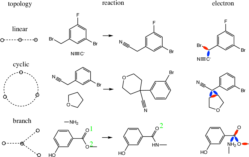
Figure 3: Different reaction topology (left) and reaction products generated by our method (middle), where the green numbers distinguish different oxide atoms. On the right, the blue lines denote new bonds formed, and the red lines denote bonds broken.

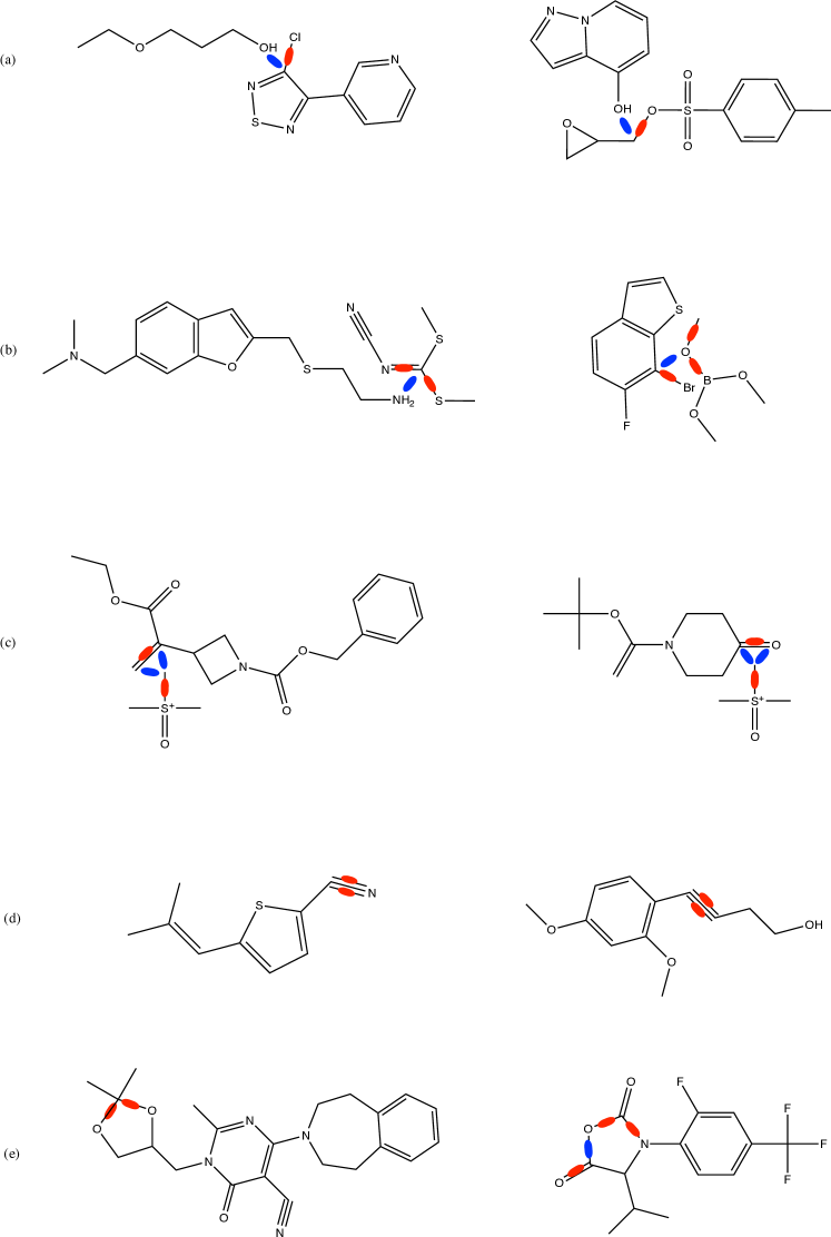
Figure 4: Extra examples of our reaction topology. (a)(b)(c)(d)(e) are samples with reaction centers (Jin et al., 2017) of linear, branch, cyclic, parallel and multi topology respectively. The red edges are bonds broken while blue edges denote bonds formed.

4.4 Accuracy on Individual Topology

In addition to the overall accuracy, we also examined our model’s performance on different types of reaction topology.

Herges (1994b) considers three types of reaction topology, namely Linear, Cyclic, Complex for the full USTPO dataset as an organizing principle for the known reactions. Nevertheless, for the USTPO-MIT dataset, this will result in extremely imbalanced categories with over 99% of samples falling into the Linear topology. Inspired by the topology used in (Bradshaw et al., 2018), we select three types of representative topology, namely Single-Linear (73% of total samples), Branch (tree-structured, with 17% of total samples) and Cyclic (cyclic and complex reactions with 0.5% yet important samples) (illustrated in the left of Figure  3).

We compare our method with the Transformer (both base and augmented versions), Symbolic, and ELECTRO (Bradshaw et al., 2018). Results in Table 3 show that our model achieved superior or performed on par with the four comparison baselines on all the three types of topology. For example, our method achieved the best accuracy on the Linear, Branch, and Cyclic, except obtaining slightly lower accuracy than that of Symbolic on Linear and that of Transformer-augmented on Cyclic. On the other hand, the ELECTRO performed the worst on the Linear topology, while Symbolic achieved the best on Linear type but lower accuracy on the Branch and Cyclic. Also, although Transformer-augmented obtained the highest accuracy on the Cyclic, but it obtained lower accuracy than our method on the other two categories, namely Linear and Branch. These results suggest that our method performs well over all the individual topology types.

4.5 Topology and Prediction Visualization

Figure 3 visualizes some generated reaction products that follow the three types of topology as described above. The left column of Figure 3 depicts the three types of topology, namely Linear, Cyclic, and Branch. The middle two columns show the reaction of transforming reactant on the left to the product on the right, which is correctly predicted by our method. The right column of the figure presents the corresponding electron flows captured by our model during the reactions, where the blue lines denote new bonds formed and the red lines denote bond broken.

Figure 3 indicates that our model can not only predict reactions from various types of topology, but also clearly show the electron flows that result in the final reaction products.

In Figure 4, we also depict additional cases of our model predictions. In addition to the aforementioned three topology, we here also list parallel and multi topology, covering all of our taxonomy. Parallel topology refers to the reactions where there are parallel edges breaking or forming, and Multi are those with multiple reaction centers, each representing a series of bond forming and breaking.

4.6 Interpretability

Bradshaw et al. (2018) show intuitive interpretability of their model due to the prediction of mechanism. Since our model embraces predicting the pseudo-mechanism, namely the electron flows during the reactions, our predictions are also easy for chemists to interpret.

Figure 5: A reaction correctly predicted by our model. Our model predicts the direction and the number of electron flows, which are denoted by arrow pushing and real values respectively. These predictions clearly show what caused the bond making and breaking during the reaction, thus it is much easier for chemists to interpret. The product in the green box is the ground truth, which is predicted correctly, and we also predicted the byproducts (in the purple box) at the same time when generating the whole predicted graph $\hat{G}^{p}$.

Figure 5 shows a reaction with non-linear topology predicted by our model, where the green box is the ground truth, which is predicted by our model correctly. Note that, our method also predicted the byproducts (shown in purple box) at the same time when generating the whole predicted graph $\hat{G}^{p}$.

Figure 5 shows that our model correctly predicted the bond formation (in blue) and bond breaking (in red). This is explained by the predicted number next to the pushing array, indicating the predicted edge change $\hat{e}_{ij}$ as discussed in Equation 13. Recall from Section 3.2.2 that by rounding $\hat{e}_{ij}$ to discrete values $\hat{e}^{p}_{ij}$, as described in Equation 15, we obtain the bond changes.

It is worth noting that our model predicts the electron re-distribution around all atoms in the reactants. Hence, it infers side products. Note that the byproduct drawn as dimethylsulfoxide (DMSO) does not appear in the ground truth record for this reaction, as the dataset only contains “major” reaction products. Byproducts are all speculative and predicted without any labeled training examples. To this end, following literature, we do not evaluate the side products.

5 Conclusion and Future Work

We formulated chemical reaction as a simultaneous electron redistribution problem and solved it with a novel multi-pointer decoding network. This results in the first non-autoregressive electron flow model for reaction prediction, which captures the simultaneous bond making and breaking in molecules in one shot. We empirically verified that our method achieved superior top-1 accuracy and at least 27 times inference speedup over the state-of-the-art methods.

Possessing superior predictive performance, parallel computation, and intuitive interpretability makes our strategy NERF an appealing solution to practical learning problems involving chemical reactions.

In the future, we will investigate the potential of applying our framework to more complicated settings such as stereochemistry.

6 Acknowledgements

This project was supported by the Natural Sciences and Engineering Research Council (NSERC) Discovery Grant, the Canada CIFAR AI Chair Program, collaboration grants between Microsoft Research and Mila, Samsung Electronics Co., Ldt., Amazon Faculty Research Award, Tencent AI Lab Rhino-Bird Gift Fund and a NRC Collaborative R&D Project (AI4D-CORE-06). This project was also partially funded by IVADO Fundamental Research Project grant PRF2019-3583139727.

References

- Bradshaw et al. (2018) Bradshaw, J., Kusner, M. J., Paige, B., Segler, M. H., and Hernández-Lobato, J. M. A generative model for electron paths. arXiv preprint arXiv:1805.10970, 2018.
- Coley et al. (2017) Coley, C. W., Barzilay, R., Jaakkola, T. S., Green, W. H., and Jensen, K. F. Prediction of organic reaction outcomes using machine learning. ACS central science, 3(5):434–443, 2017.
- Coley et al. (2019) Coley, C. W., Jin, W., Rogers, L., Jamison, T. F., Jaakkola, T. S., Green, W. H., Barzilay, R., and Jensen, K. F. A graph-convolutional neural network model for the prediction of chemical reactivity. Chemical science, 10(2):370–377, 2019.
- Corey & Wipke (1969) Corey, E. and Wipke, W. T. Computer-assisted design of complex organic syntheses. Science, 166(3902):178–192, 1969.
- Do et al. (2019) Do, K., Tran, T., and Venkatesh, S. Graph transformation policy network for chemical reaction prediction. pp. 750–760, 07 2019. doi: 10.1145/3292500.3330958.
- Herges (1994a) Herges, R. Coarctate transition states: the discovery of a reaction principle. Journal of Chemical Information and Computer Sciences, 34(1):91–102, 1994a.
- Herges (1994b) Herges, R. Coarctate transition states: the discovery of a reaction principle. Journal of Chemical Information and Computer Sciences, 34(1):91–102, 1994b.
- Herges (2015) Herges, R. Coarctate and pseudocoarctate reactions, stereochemical rules. The Journal of organic chemistry, 80, 09 2015. doi: 10.1021/acs.joc.5b01959.
- Jin et al. (2017) Jin, W., Coley, C. W., Barzilay, R., and Jaakkola, T. Predicting organic reaction outcomes with weisfeiler-lehman network. Advances in Neural Information Processing Systems, 2017-December(Nips):2608–2617, 2017. ISSN 10495258.
- Kayala & Baldi (2011) Kayala, M. A. and Baldi, P. F. A machine learning approach to predict chemical reactions. In Shawe-Taylor, J., Zemel, R. S., Bartlett, P. L., Pereira, F., and Weinberger, K. Q. (eds.), Advances in Neural Information Processing Systems 24, pp. 747–755. 2011.
- Kingma & Ba (2014) Kingma, D. P. and Ba, J. Adam: A method for stochastic optimization. arXiv preprint arXiv:1412.6980, 2014.
- Kingma & Welling (2013) Kingma, D. P. and Welling, M. Auto-Encoding Variational Bayes. arXiv e-prints, art. arXiv:1312.6114, December 2013.
- Landrum (2016) Landrum, G. Rdkit: Open-source cheminformatics software, 2016.
- Lowe (2012) Lowe, D. M. Extraction of chemical structures and reactions from the literature. 2012.
- Paszke et al. (2019) Paszke, A., Gross, S., Massa, F., Lerer, A., Bradbury, J., Chanan, G., Killeen, T., Lin, Z., Gimelshein, N., Antiga, L., et al. Pytorch: An imperative style, high-performance deep learning library. In Advances in Neural Information Processing Systems, pp. 8024–8035, 2019.
- Qian et al. (2020) Qian, W. W., Russell, N. T., Simons, C. L., Luo, Y., Burke, M. D., and Peng, J. Integrating deep neural networks and symbolic inference for organic reactivity prediction. 2020.
- Rong et al. (2020) Rong, Y., Bian, Y., Xu, T., Xie, W., Wei, Y., Huang, W., and Huang, J. Grover: Self-supervised message passing transformer on large-scale molecular data, 2020.
- Sacha et al. (2020) Sacha, M., Błaż, M., Byrski, P., Włodarczyk-Pruszyński, P., and Jastrzebski, S. Molecule edit graph attention network: Modeling chemical reactions as sequences of graph edits, 2020.
- Schlichtkrull et al. (2018) Schlichtkrull, M., Kipf, T. N., Bloem, P., Van Den Berg, R., Titov, I., and Welling, M. Modeling relational data with graph convolutional networks. In European Semantic Web Conference, pp. 593–607. Springer, 2018.
- Schwaller et al. (2018) Schwaller, P., Gaudin, T., Lanyi, D., Bekas, C., and Laino, T. “found in translation”: predicting outcomes of complex organic chemistry reactions using neural sequence-to-sequence models. Chemical science, 9(28):6091–6098, 2018.
- Schwaller et al. (2019) Schwaller, P., Laino, T., Gaudin, T., Bolgar, P., Hunter, C. A., Bekas, C., and Lee, A. A. Molecular transformer: A model for uncertainty-calibrated chemical reaction prediction. ACS Central Science, 5(9):1572–1583, 2019.
- Segler & Waller (2017a) Segler, M. H. and Waller, M. P. Modelling chemical reasoning to predict and invent reactions. Chemistry–A European Journal, 23(25):6118–6128, 2017a.
- Segler & Waller (2017b) Segler, M. H. and Waller, M. P. Neural-symbolic machine learning for retrosynthesis and reaction prediction. Chemistry–A European Journal, 23(25):5966–5971, 2017b.
- Shi et al. (2020) Shi, C., Xu, M., Guo, H., Zhang, M., and Tang, J. A graph to graphs framework for retrosynthesis prediction. In ICML, pp. 8818–8827, 2020.
- Sohn et al. (2015) Sohn, K., Lee, H., and Yan, X. Learning structured output representation using deep conditional generative models. pp. 3483–3491, 2015.
- Struble et al. (2020) Struble, T. J., Alvarez, J. C., Brown, S. P., Chytil, M., Cisar, J., DesJarlais, R. L., Engkvist, O., Frank, S. A., Greve, D. R., Griffin, D. J., Hou, X., Johannes, J. W., Kreatsoulas, C., Lahue, B., Mathea, M., Mogk, G., Nicolaou, C. A., Palmer, A. D., Price, D. J., Robinson, R. I., Salentin, S., Xing, L., Jaakkola, T., Green, W. H., Barzilay, R., Coley, C. W., and Jensen, K. F. Current and future roles of artificial intelligence in medicinal chemistry synthesis. Journal of Medicinal Chemistry, 63(16):8667–8682, 2020.
- Vaswani et al. (2017) Vaswani, A., Shazeer, N., Parmar, N., Uszkoreit, J., Jones, L., Gomez, A. N., Kaiser, L. u., and Polosukhin, I. Attention is all you need. In Guyon, I., Luxburg, U. V., Bengio, S., Wallach, H., Fergus, R., Vishwanathan, S., and Garnett, R. (eds.), Advances in Neural Information Processing Systems 30, pp. 5998–6008. Curran Associates, Inc., 2017.
- Vinyals et al. (2015) Vinyals, O., Fortunato, M., and Jaitly, N. Pointer networks. In Advances in neural information processing systems, pp. 2692–2700, 2015.
- Wei et al. (2016) Wei, J. N., Duvenaud, D., and Aspuru-Guzik, A. Neural networks for the prediction of organic chemistry reactions. ACS central science, 2(10):725–732, 2016.
- Weininger (1988) Weininger, D. Smiles, a chemical language and information system. 1. introduction to methodology and encoding rules. Journal of chemical information and computer sciences, 28(1):31–36, 1988.
- You et al. (2019) You, J., Ying, R., and Leskovec, J. Position-aware graph neural networks, 2019.