Embracing Uncertainty in “Small Data” Problems: Estimating Earthquakes from Historical Anecdotes

Abstract

Improving understanding of current seismic risk is often dependent on developing a more complete characterization of earthquakes that have occurred in the past, and in particular before the development of modern sensing equipment in the middle of the twentieth century. However, accounts of such events are typically anecdotal in nature, limiting efforts to model them to more heuristic approaches. To address this shortfall, we develop a framework based in Bayesian inference to provide a more rigorous methodology for estimating pre-instrumental earthquakes. By directly modeling accounts of resultant tsunamis via probability distributions, the framework allows practitioners to make principled estimates of key characteristics (e.g., magnitude and location) of historical earthquakes. To illustrate this idea, we apply the methodology to the estimation of an earthquake in Eastern Indonesia in the mid 19th century, the source of which is currently the subject of considerable debate in the geological community. The approach taken here gives evidence that even “small data” that is limited in scope and extremely uncertain can still be used to yield information on past seismic events. Moreover, sensitivity bounds indicate that the results obtained here are robust despite the inherent uncertainty in the observations.

Keywords: Bayesian inference, Estimation of historical events, Tsunami modeling, Seismic risk assessment, Uncertainty quantification, Sensitivity analysis.
MSC2020: 62P35, 86A22

1 Introduction

The geologically recent mega-thrust earthquakes and giant tsunamis in Indonesia (2004) and Japan (2011) as well as the seismic catastrophes in Haiti (2010) and China (2008) each occurred in regions previously mapped as having “low” seismic hazard. One reason for this is because hazard assessments relied largely on instrumental data only available since the mid-1900s [58]. Historical records and geological evidence of seismic events exist in each of these regions, but they were not adequately accounted for due to the uncertainty that is inherent to such data sources [42]. For example, tsunami deposits were documented on the Sendai Plain before the 2011 Japan mega-thrust earthquake [39], but were not considered in risk assessments, such as the retrofitting of the nuclear power plant. These recent seismic and tsunami disasters motivate us to push beyond the geologically limited time window of instrumentally recorded earthquakes to find new ways of quantifying unconventional data sources for earthquake locations and magnitudes.

Resilience to tsunamis and other seismic hazards requires learning from what has happened in the past – incorporating all available data and records (even from uncertain sources) – and thereby reducing the negative impact of future events through more comprehensive hazards education and preparedness strategies [64]. While evidence of previous earthquake and tsunami events can be found in the geological record, such as deposits left by previous tsunami events [60], damage to coral reefs [38, 16], and sediment cores of turbidites [21], much information on past events is available in the form of textual accounts in historical records such as the recently translated Wichmann catalog [68, 69, 26] and other sources [51, 4, 41, 49] for Indonesia, North and South America (see [56, 11, 32] for example), and many other locations in Asia and throughout the world. Issues and concerns about the accuracy and validity of historical records illustrate a shift from the question “can we quantify what happened?” to “can we make a principled estimate of the uncertainties around what happened?”.

While developing rigorous and reproducible estimates of historical events from textual and anecdotal accounts presents a number of obvious challenges, recent efforts to do so illustrate both the promise of these data sources as well as the imperative of incorporating all available historical data into the modern understanding of seismic risk. For example the western Sunda Arc experienced the great Sumatran earthquake and Indian Ocean tsunami of 2004, which claimed more lives than any other tsunami in recorded history [2]. Most of the world was surprised by the event because it had been forty years since an earthquake or tsunami of that magnitude had occurred anywhere on Earth, and much longer since one had happened in a densely populated area like Indonesia. However, several studies prior to the event used historical and geological records to identify the seismic risk in this region [43, 19, 25, 70, 24]. (Several studies since have also identified evidence of large tsunamis in the region – see, for example, [38, 47, 54].) Unfortunately, due to the uncertain nature of historical accounts, these studies did not quantify or provide uncertainties for their predictions and hence their results were not actively incorporated into hazard assessments for the region. In addition, this scientific research did not move “downstream” very far, and did nothing to increase resiliency to tsunami hazards in the Indian Ocean region as most of those in harm’s way did not know what a tsunami was, let alone that they were at extreme risk for one [31].

In effect, in a field awash with “big” data – modern automated instrumentation – reconstructions of seismic and tsunami events from historical accounts failed to have a direct impact on forecasting and mitigation efforts because they relied on data that was “small,” i.e., sparse, highly uncertain, centuries old, and in some cases textual or anecdotal in nature. In addition, the methods used to infer the causative event were largely ad-hoc, so the resulting inference to characterize previous events and hence the prediction of future events was necessarily qualitative. This is useful to indicate the potential for a seismic hazard, but is of little quantitative use for policy decisions relevant to hazard assessment. It is therefore desirable to develop a more rigorous and reproducible methodology that can both leverage the promise of these historical data to provide new insights about seismic history, informing understanding of the current status of elastic strain accumulation of the relevant faults, while also being honest about what it cannot tell us due to the inherently uncertain nature of the data.

In this paper, we apply the Bayesian approach to inverse problems [30, 59, 17] to address this issue. A Bayesian framework is a natural fit because the chief problem we face is uncertainty in the data; the resulting posterior distribution will therefore provide estimates of the most likely values of, but also the uncertainties that surround, the seismic parameters we would like to estimate, e.g., the magnitude and location of the historical earthquake in question. Here the numerical resolution of partial differential equations (PDEs) describing tsunami wave propagation provides a “forward map” which can be “inverted” starting from our historical data to develop the posterior distribution. While the Bayesian framework has been used in the past to address problems in seismicity (see [7, 36, 20] for a few examples), our study is the first that we know of to apply the approach to inference of pre-instrumental events. Our focus here is on an initial case study concerning the reconstruction of the 1852 Banda arc earthquake and tsunami in Indonesia detailed in the recently translated Wichmann catalog of earthquakes [26, 69] and from contemporary newspaper accounts [61]. We refer the reader to [52], which describes the approach to estimating the 1852 event from a more geological perspective, as well as to the graduate thesis [53].

The rest of the article is organized as follows: Section 2 describes the dataset that we will use, its limitations, and the associated challenges of drawing conclusions from it. In Section 3, we detail how we adapt the Bayesian framework to the problem. In Section 4, we outline how we apply the approach to the 1852 Banda Arc earthquake and tsunami. Section 5 describes the results of the inference for the 1852 event and bounds on the sensitivity and uncertainty of our analysis. Section 6 outlines conclusions of geological relevance for the 1852 event, how the methodology can be applied to other problems, and related paths for future research.

2 The Data: Historical Accounts of Tsunamis

In this section, we describe the kinds of data that will be used to infer characteristics of historical earthquakes and some of the challenges associated with doing so. We focus on textual accounts, although analogous (if perhaps less severe) interpretation issues arise with geological data such as disrupted turbidites, coral uplifts, and tsunami deposits. In particular, geological evidence of past seismic events is less uncertain, but the monetary cost of obtaining such data is prohibitive. As an example for the textual accounts, the two volumes of Arthur Wichmann’s The Earthquakes of the Indian Archipelago [68, 69] document nearly 350 years of observations of earthquakes and tsunamis for the entire Indonesian region. The observations were mostly compiled from Dutch records kept by the Dutch East India Company of Indonesia. Seismic events are included that reach west to east from the Cocos Islands to New Guinea, and north to south from Bangladesh to Timor. Although the catalogue is cited in some tsunami and earthquake literature [57, 44], it remained largely unknown to the scientific community until its translation to English and interpretation of what faults may have produced these events [26].

The Wichmann catalog documents 61 earthquakes and 36 tsunamis in the Indonesian region between 1538 and 1877. Most of these events caused damage over a broad region, and are associated with years of temporal and spatial clustering of earthquakes. However, there has not been a major shallow earthquake ($Mw\geq 8$) in Java and eastern Indonesia for the past 160 years. During this time of relative quiescence, enough tectonic strain energy has accumulated across several active faults to cause major earthquake and tsunami events reminiscent of those documented in the Wichmann catalog. The disaster potential of these events is much greater now than in the past due to an exponential growth in population and urbanization in coastal regions destroyed by past events.

2.1 The 1852 Tsunami and Historical Observations

1852, November 26, 7:40. At Banda Neira, barely had the ground been calm for a quarter of an hour when the flood wave crashed in …The water rose to the roofs of the storehouses …and reached the base of the hill on which Fort Belgica is built on.

Figure 1: An excerpt from the Wichmann catalog for the 1852 tsunami and earthquake.

The gigantic earthquake and tsunami of 1852 is perhaps the largest recorded historic seismic event of its kind in eastern Indonesia [15]. The main shock of the earthquake took place between 7 a.m. and 8 a.m. on November 26, 1852. Later that day, 9 aftershocks were felt. Aftershocks happened daily for the next 8 days and occasionally in the following months and years. For context, a map of the region is shown in Figure 2.

Figure 1 shows an excerpt from the Wichmann catalog entry for the 1852 tsunami with observations in Banda Neira, a small island in the Banda Sea west of Papua New Guinea. The account provides clear descriptors, such as locations, arrival times, wave heights, and inundation lengths that can be used to characterize the tsunami and infer the earthquake that might have caused it. Moreover, because historical observations of the tsunamis were observed in multiple, often geographically-dispersed locations (Banda Neira being just one of several for the 1852 event), even uncertain observations can be “triangulated” to provide more certain estimates of earthquake size and location.

At the same time, the excerpt also demonstrates some of the challenges associated with doing such an inference in a rigorous way: Given that these measurements were taken well before the modern era of automated and sophisticated sensing, how accurate are they? What does water rising to rooftops tell us about the event? In the next section, we describe past attempts in the natural hazards community to use observations like those above to estimate historical earthquakes.

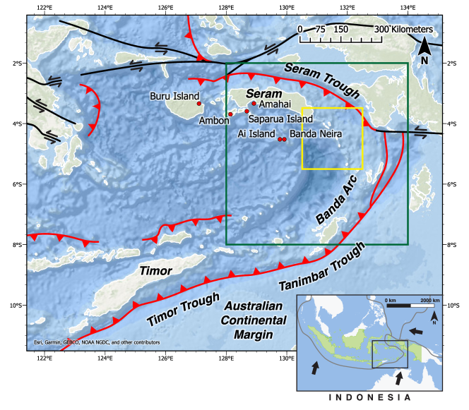
Figure 2: The seismic and geologic setting for the 1852 event. Convergent/transvergent plate boundaries are in red/black. The green rectangle indicates the region that is depicted in Figure 6. The yellow rectangle is where the posterior distribution concentrates. Locations where observations of the tsunami are used in the inversion process are labeled and indicated by a red dot.

2.2 Past Approaches to Historical Inference

Previous efforts to reconstruct pre-instrumental earthquakes have varied from a focus on the use of geological evidence (see [40, 55, 29, 38] for example) to the use of historically recorded (but not instrumental) accounts [46, 6, 35, 26, 50, 15, 23, 9, 48] as well as some combination of the two types of uncertain data (see [37] for one example). Most of these efforts, particularly those directed toward using historical records, have relied on a combination of physical intuition and a restricted number of forward simulations to match the observational data. Qualitative comparisons are then made to the historical (or geological) record, and a heuristic choice is made as to the “best” forward simulation that fits the data.

Past attempts have been made to reconstruct the earthquake that produced the 1852 tsunami using observations from the Wichmann catalog in particular. In [15], for example, the Wichmann observations were converted into estimates of wave heights, arrival times, and onshore wave runups. Nine “reasonable” candidate earthquakes were then constructed and simulated using a numerical model of tsunami propagation. The numerical results and Wichmann text were then qualitatively compared to determine which candidate event provided the “best” match, which then was declared the most likely source. This analysis indicated that the source of the 1852 event was an earthquake on the Tanimbar trough exceeding 8.4 Mw.

This approach, however, is laced with subjective judgments, particularly in terms of (i) how such uncertain observations are converted into numerical estimates (ii) which candidate earthquake sources are chosen and (iii) what constitutes the best match. Taken together, these concerns make the results difficult to justify or reproduce. Meanwhile, interpreting observations like those in Figure 1 as a single number representing arrival time or wave height is clearly too simplistic. So while such investigations have significantly improved our understanding of the historical seismicity of different regions, with modern computational resources and recent advances in algorithmic techniques, we propose a more principled approach to model observational error and incorporate it into the inversion process.

3 Bayesian Inference and Likelihood Modeling

Our approach to leveraging the data described in Section 2 in a more principled and systematic fashion involves introducing a Bayesian framework [17, 30, 10, 63], which provides a rigorous, statistical methodology for converting uncertain outputs into probabilistic estimates of model parameters. We note that while we use the earthquake example described above as a motivating example, the framework described in this section is applicable to any problem where the “data” is “small” and/or highly uncertain. In what follows, we denote the model parameters characterizing the seismic event of interest by $\mathbf{u}$, the “data” by $\mathbf{y}$, the prior measure by $p_{0}$, the forward model $\mathcal{G}$ from model parameters (e.g., earthquake magnitude and location) to observables (e.g., tsunami wave height), the likelihood by $L(\mathbf{u};\mathbf{y})\propto p(\mathbf{y}|\mathbf{u})$, and the posterior measure by $p_{post}$. See the references above for definitions of these quantities. Bayes’ Theorem provides an explicit expression for $p_{post}$ as

$$p_{post}(\mathbf{u})\propto L(\mathbf{u};\mathbf{y})p_{0}(\mathbf{u}).$$ (1)

Most critically, the Bayesian approach incorporates uncertainty at all levels of the inverse problem, an essential feature given that the data in this case clearly does not provide enough information to fully specify the model parameters – we hope that it will tell us something about the parameters, but expect that it will necessarily not tell us everything.

3.1 Likelihood Modeling

In this section, we outline our procedure for modeling noisy or anecdotal data via the likelihood. While the tsunami observations described in Section 2 provide a motivating example, the approach described here could be applied to any problem where the data has similar issues of being so ill-defined as to be anecdotal. Application to the tsunami problem is described in detail in Section 3.2 and Section 4.3.

To model the data $\mathbf{y}$ from anecdotal observations like those described in Section 2, we adopt a data augmentation approach (see, e.g., [62, 1, 65, 28]) and introduce an auxiliary variable $\mathbf{w}$ representing additional, unobserved data. Then the likelihood is given by

$$L(\mathbf{u};\mathbf{y}) \propto p(\mathbf{y}|\mathbf{u})=\int p(\mathbf{y}|\mathbf{w},\mathbf{u})p(\mathbf{w}|\mathbf{u})\,d\mathbf{w}.$$ (2)

Here, for our augmentation variable $\mathbf{w}$ we use the true value of the output (e.g., $w_{i}$ might be the true wave height while $y_{i}$ is the observed value of the wave height) and assume that uncertainty in the true value is independent of $\mathbf{u}$ so that $p(\mathbf{y}|\mathbf{w},\mathbf{u})=p(\mathbf{y}|\mathbf{w})$. In this context, we incorporate information from the anecdotal data by directly modeling $p(\mathbf{y}|\mathbf{w})$ as a function of $\mathbf{w}$ via a fixed probability density function $p_{l}(\mathbf{w})$ and assume

$$p_{l}(\mathbf{w})\propto p(\mathbf{y}|\mathbf{w}).$$ (3)

From a practical standpoint, this strategy leverages the fact that the unexpressed integration constant in (3) does not feature in the posterior distribution (1):

$$p_{post}(\mathbf{u})=\frac{\left(\int p(\mathbf{y}|\mathbf{w})p(\mathbf{w}|\mathbf{u})\,d\mathbf{w}\right)p_{0}(\mathbf{u})}{\int\left(\int p(\mathbf{y}|\mathbf{w})p(\mathbf{w}|\mathbf{u})\,d\mathbf{w}\right)p_{0}(\mathbf{u})d\mathbf{u}}=\frac{\left(\int p_{l}(\mathbf{w})p(\mathbf{w}|\mathbf{u})\,d\mathbf{w}\right)p_{0}(\mathbf{u})}{\int\left(\int p_{l}(\mathbf{w})p(\mathbf{w}|\mathbf{u})\,d\mathbf{w}\right)p_{0}(\mathbf{u})d\mathbf{u}}\,.$$

From a philosophical standpoint, this strategy represents an application of the likelihood principle [14, 8], insofar as it allocates higher values of $p_{l}(\cdot)$ for $\mathbf{w}$ that better ‘match’ the data as quantified by the function $p(\mathbf{y}|\mathbf{w})$. Section 4.3 discusses the specification of $p_{l}(\cdot)$ for tsunami characteristics.

Meanwhile, we require that true observations $\mathbf{w}$ match the forward map $\mathcal{G}(\mathbf{u})$, so we define

$$p(\mathbf{w}|\mathbf{u}) =\delta(\mathbf{w}-\mathcal{G}(\mathbf{u})),$$ (4)

where $\delta$ is the Dirac distribution centered at zero. Then plugging (3) and (4) into (2) yields

$$L(\mathbf{u};\mathbf{y}) \propto\int p_{l}(\mathbf{w})\delta(\mathbf{w}-\mathcal{G}(\mathbf{u}))\,d\mathbf{w}=p_{l}(\mathcal{G}(\mathbf{u})).$$ (5)

Remark 3.1.

If we assume the data model $\mathbf{y}=\mathbf{w}+\eta$ for additive observational noise $\eta\perp\mathbf{u}$ and $\mathbf{w}=\mathcal{G}(\mathbf{u})$ for some $\mathbf{u}$, then, denoting the probability density of $\eta$ by $p_{\eta}$, $\mathbf{w}$ has density $p_{l}(\mathbf{w}):=p_{\eta}(\mathbf{y}-\mathbf{w})$ and we have via (5)

$$L(\mathbf{u};\mathbf{y})=p_{\eta}(\mathbf{y}-\mathcal{G}(\mathbf{u})),$$ (6)

which is a popular likelihood used in Bayesian inverse problems; see, e.g., [30, Section 3.2.1] or [10, Section 1.1]. Thus, (3) is a generalization where the structure of the observational noise is left in a more implicit form.

Of course, the choice of the observation distribution $p_{l}$ in (3) is subjective, as any interpretation of the historical records described in Section 2 must be. However, the approach outlined above represents a clear improvement over the modeling of the historical data outlined in Section 2.2 in at least two ways:

• By using probability distributions rather than single values, the methodology more clearly encapsulates the uncertainty associated with the observations.

• Modeling assumptions are explicitly specified and incorporated into the methodology so that the results are rigorous and reproducible.

One might interpret the direct modeling of the likelihood distribution as repeating the approach from Section 2.2 a large number of times, with the observation distribution $p_{l}(\mathbf{w})$ representing the probability that a given modeler might interpret the observation as representing the true value $\mathbf{w}$.

In any case this represents a fruitful paradigm shift from the usual Bayesian inversion framework by allowing more direct application to problems where observational signals and noise are inextricably intertwined. A practitioner can simply model what the observations tell them via $p_{l}$ in (3) and then proceed with the usual Bayesian inference using the likelihood in (5). A direct extension of the current work would be to implement this approach for other types of geological evidence such as coral uplift, sediment cores, and disrupted turbidites, but the overall framework can be leveraged by problems outside of seismic inversion as well.

3.2 Example: Application to Banda Neira

In this section, we walk through our approach to modeling the historical account described in Figure 1 for the 1852 tsunami in Banda Neira. The record includes observations of arrival time (the time interval between shaking and the arrival of the first tsunami wave), wave height (the vertical height of the wave above sea level), and inundation length (the distance that the wave reached onshore). We identify observation distributions for each observation type as follows:

• Arrival time. The text in this case states “barely had the ground been calm for a quarter of an hour when the flood wave crashed in.” This clearly implies using 15 minutes as the anticipated arrival time of the wave at Banda Neira. However, it is noted in other locations that the shaking lasted for at least 5 minutes, while the computational model used in the forward model here assumes an instantaneous rupture. Hence we build into the observation distribution a skew toward longer times with a mean of 15 minutes. This is done with a skew-normal distribution with a mean of 15 minutes, standard deviation of 5 minutes, and skew parameter 2.

• Wave height. As noted above, the historical account says “the water rose to the roofs of the storehouses.” Assuming standard construction for the time period for the homes (and storehouses), we can assume the water rose at least 4 meters above standard flood levels, as most buildings of the time were built on stilts and had steep, vaulted roofs. Based on the regular storm activity in the region we can expect that with high tide, and normal seasonal storm surge, the standard flood level was also approximately 2 meters in this region. This leads us to select a normally distributed observation distribution for wave height with a mean of $6.5m$ and standard deviation of $1.5m$, allowing for reasonable probability of wave heights in the range from $3m$ to $9m$.

• Inundation length. Here the account states that the water “reached the base of the hill on which Fort Belgica is built.” To quantify the wave reaching the base of the hill, we measured the distance from 20 randomly selected points along the beach to the edge of said hill in arcGIS (https://www.arcgis.com/). The mean of these measurements was 185 meters, with a standard deviation of roughly 65 meters. Thus we choose a normal distribution with those parameters. Without more detailed information about the coastline, and a direct idea of the direction of the traveling wave, we could not be more precise with regard to the inundation.

The observation distributions for other accounts of the 1852 tsunami and assembly of these individual distributions into a full observation distribution and likelihood are described in Section 4.3.

4 Application to the 1852 Banda Sea Earthquake and Tsunami

As noted in Section 3, Bayesian inference requires two inputs: (i) the prior distribution and (ii) the likelihood distribution, which in our application consists of a forward model composed with an observation distribution. In addition, we need a numerical method to estimate key quantities from the posterior measure. In this section, we describe how each of these components was developed for the problem of estimating the earthquake that caused the 1852 Banda Sea tsunami.

4.1 Earthquake Parameterization and Prior Distribution

To conduct Bayesian inference, we need to define a set of model parameters to estimate. The canonical parameterization of an earthquake is the nine-parameter Okada model [45], which describes the earthquake rupture as a sliding rectangular prism describing the location (latitude, longitude, depth), orientation (strike, rake, dip), and size/magnitude (length, width, slip) of the rupture. However, in practice these parameters are often highly correlated – for example, the rectangle typically has a certain range of aspect ratios, rake is near $90\degree$ for most subduction zone events (like that considered in this setting), and depth, strike, and dip can mostly be determined from latitude and longitude for major subduction zones via available instrumental data. Also, while a justifiable prior on the size parameters would be complicated to assemble, they can be estimated from earthquake magnitude, which famously follows the Gutenberg-Richter (exponential) distribution. With all of these considerations in mind, we settled on a reparameterization of the Okada model consisting of the following six parameters: (1) latitude, (2) longitude, (3) depth offset (the difference in depth from the expected depth of the subduction interface given the latitude-longitude location), (4) magnitude, and (5-6) $\Delta\log$ length and $\Delta\log$ width (a logarithmically scaled difference in length and width from the expected values for the given magnitude).

The prior distributions on latitude, longitude, and depth offsets were determined from the Slab2 dataset [27] which incorporates modern instrumental data to map out major subduction zones globally. The prior distribution on magnitude was taken from the Gutenberg-Richter distribution, truncated to reasonable maximum (9.5) and minimum (6.5) values. The priors on $\Delta\log$ length and $\Delta\log$ width were taken to be normal distributions with mean zero and standard deviation computed from historical earthquake data cataloged in [66] and from recent major events from the global USGS dataset. For further details on development of the prior distributions including geophysical considerations, we refer the reader to [52] (see also [53]). The resulting prior distributions are summarized in Table 1. The prior on latitude and longitude is shown in the left-hand plot on Figure 6 while the priors for the remaining four parameters are shown in green in Figure 5. We note that the prior distributions on the magnitude, $\Delta\log$ length and $\Delta\log$ width are universally applicable to other earthquakes, whereas the prior distributions on the latitude, longitude and depth offset, while derived from the Slab2 dataset, are specific to the subduction zone in question.

Table 1: Prior distributions for the 1852 Banda Arc earthquake

Parameter name(s)	Kind	Distribution Parameters
Latitude & longitude	Pre-image of truncated normal via depth	$\mu=$ 30km, $\sigma=$ 5km, $(a,b)=$ (2.5km,50km)
Depth offset	Normal	$\mu=0$, $\sigma=$ 5km
Magnitude	Truncated exponential	$\lambda=.5$, $(a,b)=$ (6.5,9.5)
$\Delta\log L$	Normal	$\mu=0$, $\sigma=.188$
$\Delta\log W$	Normal	$\mu=0$, $\sigma=.172$

4.2 Forward Model

In Bayesian estimation, the forward model $\mathcal{G}$ takes in model parameters and outputs observables. For the earthquake estimation problem the forward model maps the earthquake parameters described in Section 4.1, modeling the resulting seafloor deformation via the Okada model [45], and then simulating tsunami generation and propagation to produce wave arrival times, wave heights, and inundation lengths. This is accomplished using the GeoClaw software package [33, 34, 22, 3]. GeoClaw computes the seafloor deformation and then simulates the tsunami via a finite-volume solver for the nonlinear shallow water partial differential equations. Approximating the posterior distribution required running the forward model thousands of times, so that implementing GeoClaw for this problem required developing a software package to automate setting it up and running it as well as several steps to carefully optimize its performance. In addition, because the events under consideration were large and the faults in the region are not rectangular (see Figure 2), approximation via a single rectangle (the default Okada model) was not physically accurate. To compensate an algorithm was developed to split the event into multiple rectangles oriented along the fault lines. Accurate tsunami simulation also required substantial effort to find and integrate data from several sources to develop more refined bathymetric data (i.e., seafloor topography) for the study region. Additional details on the many geophysical considerations in each of these steps can be found in [52, 53].

4.3 Observation Distributions and Likelihood

In Section 3.2, we provided a detailed description of our process in developing the observation distribution for historical accounts of the 1852 tsunami for observations in Banda Neira. We had usable accounts for this tsunami in eight other locations; at one (as in Banda Neira) we could estimate first wave arrival time, maximum shoreline wave height, and maximum inundation length, while at the other seven locations we could estimate only maximum wave height. This resulted in 13 total observations; the resulting observation distributions $p_{l}^{(j)},j=1,\dots,13$ are shown in Figure 3. Each was constructed in a very similar manner to that described above for Banda Neira. We note that the current investigation has assigned each observation to a single latitude-longitude location based on the historical record. Such a specific assignment is reasonable only if the likelihood distributions are sufficiently wide to account for bathymetric and model dependent resolution differences along the coastline which is a reasonable assumption, although certainly not one that is guaranteed. In future studies we will address this issue by weighting the wave heights and arrival times from a collection of nearby locations.

The total observation distribution $p_{l}$ used to define the likelihood in (5) is computed as the product of these individual observational distributions, i.e.,

$$p_{l}(\tilde{\mathbf{y}})=\Pi_{j=1}^{13}p_{l}^{(j)}(\tilde{\mathbf{y}}).$$ (7)

under the assumption that the error in each observation is independent of the others. Critically, this does not assume that the observations themselves are independent of one another, as the observations are connected via the forward model – if the wave height is high in one location, for example, it is likely to be high at all locations as the earthquake is likely larger than average. We only assume that the mistakes made by individual observers, or equivalently our (mis)interpretation of the written record for each observation, are independent. This is still somewhat questionable if, for example, observers tend to systematically over- or underestimate the size of a wave. In an attempt to mitigate these concerns, we rely only on observations with some quantifiable measurements. Moreover a more complicated construction of the total likelihood is not justifiable from the lack of detailed observations we have to work with, so we have chosen to take the most simplified approach without making additional assumptions about the structure of the likelihood.

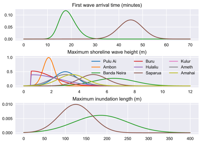
Figure 3: 1852 Banda arc tsunami observation densities $p_{l}^{(j)}$ for the 13 observations at 9 locations. Each observation density represents an interpretation of the Wichmann catalog description. The same color scheme is used for all 3 types of observations, but only Banda Neira and Saparua included wave arrival time and inundation length.

4.4 Posterior Sampling via Markov Chain Monte Carlo

As noted in Section 3, the outcome of Bayesian inference is the posterior probability distribution. Computing this distribution in practice requires computing the normalization constant $Z$ in (1), an integral that can be difficult to evaluate in practice. We therefore seek to draw samples from the posterior distribution using Markov Chain Monte Carlo (MCMC) methods. Because we did not have an adjoint solver for this PDE-based forward map, gradient-based methods like Hamiltonian Monte Carlo were not available. We therefore employed random walk-style Metropolis-Hastings MCMC; a diagonal covariance structure was used for the proposal kernel with the step size in each of the six parameters tuned to approximate the optimal acceptance rate of roughly $0.23$ [17, Section 12.2]. The final standard deviations for the random walk proposal kernel are given in the GitHub repository (see Section 6). Chains, particularly when initialized in different regions of the parameter space, sometimes got stuck in places with low posterior probability. We therefore conducted periodic importance-style resampling according to posterior probability (see [12]); this resampling does not maintain invariance with respect to the posterior measure, but provides a mechanism to “jump” trapped samples from poorly-performing regions of the parameter space to regions given more weight by the posterior distribution. To minimize any bias from the resampling steps, the approximate posterior was ultimately assembled from samples collected after a suitable burn in period following the last resampling step (see Section 5.1). The resulting algorithm is summarized in Algorithm 1.

Algorithm 1 (MCMC as Applied to the 1852 Banda Sea Tsunami Problem)

1:Choose number of chains $M$, resampling rate $N$, proposal covariance $C$, and initial parameters $\mathbf{u}_{0}^{(i)},i=1,\dots,M$.

2:for $k\geq 0$ do

3:     for $i=1,\dots,M$ do

4:         Propose $\tilde{\mathbf{u}}^{(i)}=\mathbf{u}_{k}^{(i)}+\eta,\eta\sim N(0,C)$

5:         Run Geoclaw to compute likelihood $L(\tilde{\mathbf{u}}^{(i)};\mathbf{y})$ according to (5) and (7).

6:         Compute un-normalized posterior $p_{post}(\tilde{\mathbf{u}}^{(i)})$ from (1).

7:         Set $\mathbf{u}_{k+1}^{(i)}:=\tilde{\mathbf{u}}^{(i)}$ with probability $\min\{1,p_{post}(\tilde{\mathbf{u}}^{(i)})/p_{post}(\mathbf{u}_{k}^{(i)})\}$.

8:         Otherwise take $\mathbf{u}_{k+1}^{(i)}:=\mathbf{u}_{k}^{(i)}$.      

9:     If $k\mod N=0$, resample $\mathbf{u}_{k}^{(i)}\sim\Sigma_{j}p_{post}(\mathbf{u}_{k}^{(j)})\delta\left(\mathbf{u}_{k}^{(j)}\right)/\Sigma_{l}p_{post}(\mathbf{u}_{k}^{(l)}),i=1,\dots,M$.

10:     $k\to k+1$.

5 Results for the 1852 event

In this section, we describe the results of the Bayesian inference of the 1852 Banda Arc earthquake and tsunami using the approach described in Section 4. We first outline behavior of the MCMC chains (Section 5.1), then in Section 5.2 we describe the structure of the computed posterior distribution and some conclusions of geological significance that can be drawn from it. Finally, we provide some results on the sensitivity of the posterior distribution to the choice of likelihood function in Section 5.3.

5.1 Sampling and Convergence

To ensure that all viable seismic events were considered, we initialized 14 MCMC chains at locations around the Banda arc with initial magnitudes of either $8.5$ or $9.0$ Mw. Additional chains were initialized at $8.0$ Mw; however, these were quickly discarded as they consistently failed to generate a sufficiently large wave to reach all of the observation points (Figure 2) and therefore produced likelihoods of zero probability. Each chain was initialized with the other sample parameters (depth offset etc.) set to zero. Each of the 14 chains was run for 24,000 samples, for a total of 336,000 samples. These samples were computed using the computational resources available through BYU’s Office of Research Computing, consuming a total of nearly 200,000 core-hours in all.

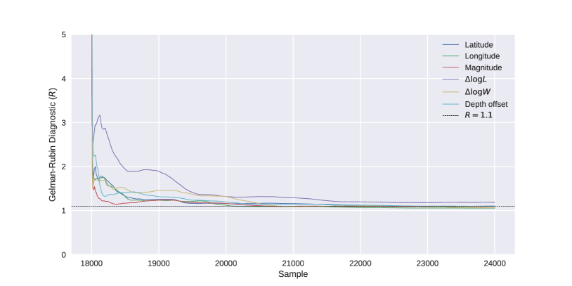
Figure 9: The Gelman-Rubin diagnostic $\hat{R}$ for each of the six sampling parameters.

About two thirds of the chains converged from their disparate initial conditions to a similar region in the parameter space that ultimately represented the bulk of the posterior distribution. However, the remaining third of the chains became trapped by geographic barriers in a region of parameter space with much lower posterior probability (roughly $\exp(-5)$ to $\exp(-10)$ times the probability of the samples in the first region). For this reason, as noted in Section 4.4, after 6,000 samples we resampled the chains using importance sampling to give each a chance to jump to regions of higher probability. Resampling was conducted twice more at samples 12,000 and 18,000. However, the range of posterior values was much smaller at the second two resampling steps and so resampling had a less pronounced impact. Since the resampling adds a small amount of bias to the posterior once the samples are in equilibrium, these latter two resampling steps were in retrospect probably not warranted. To minimize their effect, we therefore use only the last 5,000 steps from each chain (assuming a 1,000 sample ”burn in” after the last resampling), making a dataset of 70,000 samples from which we approximate the posterior distribution. The results of the sampling are shown in Figure 9; the figure shows 100-sample rolling averages across all chains (blue) plus or minus their standard deviations (black) for each parameter as well as the points at which resampling was done (red) and the samples included in the final approximate posterior (green). The figure shows the large jumps associated with the first resampling, smaller jumps at the second resampling, and almost no effect in the third resampling; the chains appear to have reached approximate equilibrium by about midway through the sampling so that the final 5,000 samples should provide a good representation of the posterior measure as a whole. To check this, we compute the Gelman-Rubin diagnostic $\hat{R}$ from [18, 5, 17] for each of the six parameters; to ensure that the resampling does not unduly bias the results, we compute the diagnostic using the $6,000$ samples from after the last resampling step. Each of the six parameters have $\hat{R}<1.2$ (all but one is below $1.1$), a common criterion indicating convergence, see, e.g. [5]. A plot of $\hat{R}$ is shown in Appendix A.

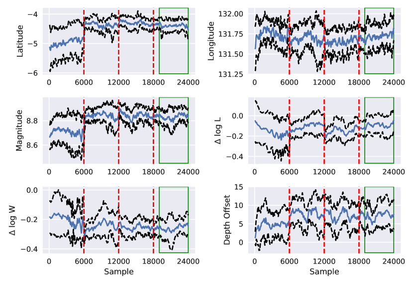
Figure 4: MCMC sampling by parameter. 100-sample rolling averages across all chains are shown in blue. Black lines show the rolling averages $\pm$ their standard deviations. Resampling points are marked with red lines. The green box shows samples used in the final computed posterior.

5.2 Posterior Structure

The resulting approximate posterior structure shows that, even though the individual observations were highly uncertain, taken together they provide strong evidence for several conclusions of geophysical significance. First, as shown in Figure 5, the 1852 earthquake was likely very large, with magnitude greater than 8.5 Mw. This is because the tsunami modeling consistently – over hundreds of thousands of trials – indicated that an earthquake would need to be at least this large to generate observable waves at each of the nine observation locations. This is an important conclusion because no earthquake of this magnitude has been recorded in the Banda Sea during the period of instrumental data (since approximately 1950). Second, as shown in Figure 6, while the prior distribution considered events all along the Banda Arc, the observations imply that the centroid for the 1852 earthquake likely occurred in a narrow region near 4.5°S, 131.5°E, which is situated in a shallow part of the subduction interface. This is the “triangulation effect” – because the observations were in different locations, the different wave heights and arrival times allowed the model to constrain the location of the event even though each observation was highly uncertain if considered individually.

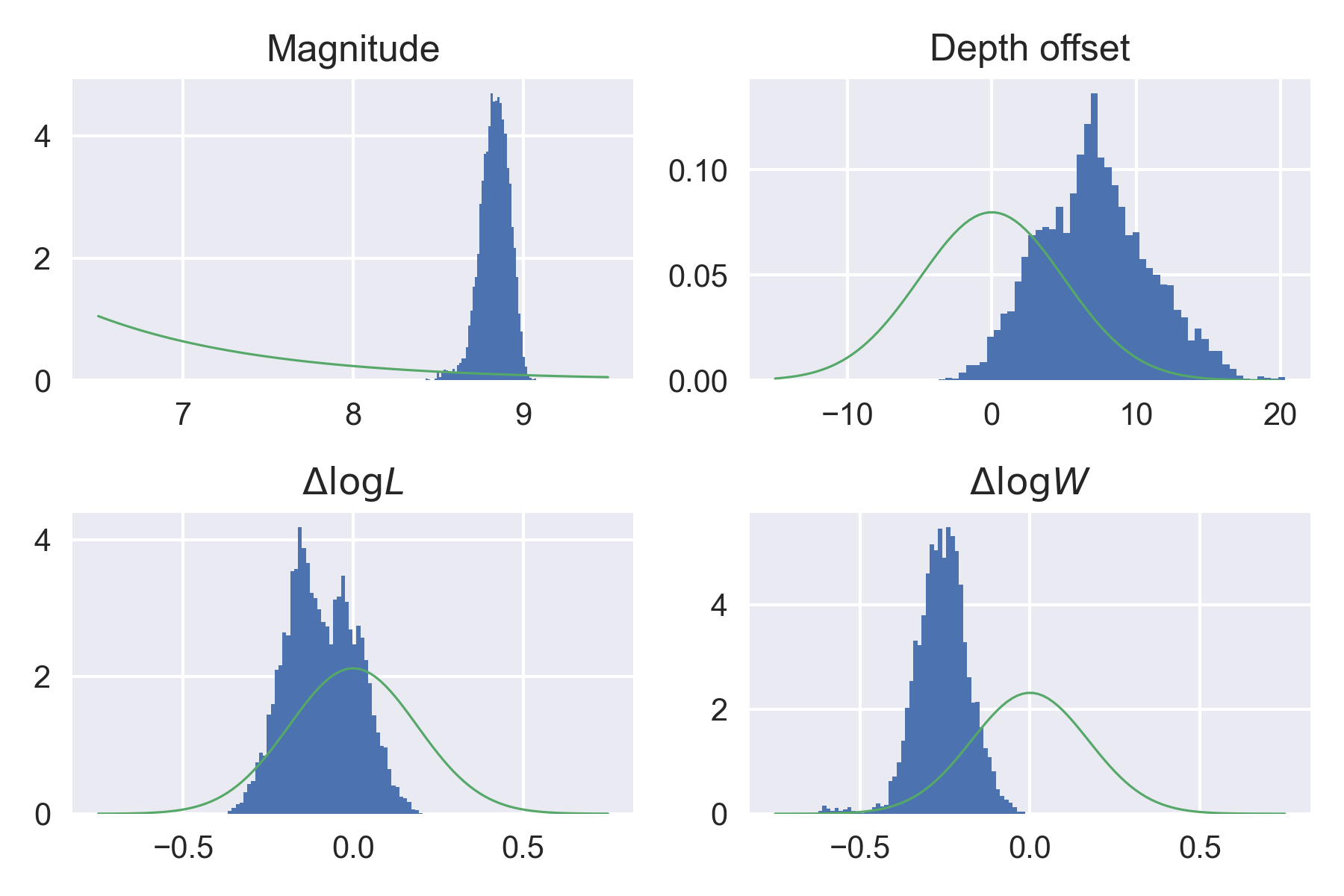
Figure 5: Magnitude, depth offset, $\Delta\log L$, and $\Delta\log W$ posterior histograms and associated prior distribution densities (green).

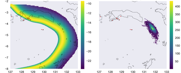
Figure 6: Centroid latitude/longitude for the prior (left) and posterior (right) distributions, showing concentration in a narrow region of the Banda arc. Observation locations in red.

Insight into the behavior of the model can be gleaned from the posterior predictive distributions shown in Figure 7. These distributions are the histograms of the observables associated with the posterior distribution. Overlaid on the plots are the observation distributions as well as the observables associated with the approximate maximum a posteriori (MAP) and maximum likelihood estimator (MLE) points of the distribution (the maxima among the posterior samples). The match or mismatch between the histograms and the observation distributions show where the model was able to match the observations well, and where it was not. The histograms can also be interpreted as predictions of what communities in these locations might be expected to experience – the wave heights, arrival times, and inundations – should a similar event happen in the future. For instance, if an event of this magnitude occurred in the same location on the Banda arc, we anticipate a wave of approximately $2.5m$ to reach the populous city of Ambon (approximately 300,000 people). For those living in the bay of Ambon, this is a potentially powerful tool for probabilistic hazard assessment.

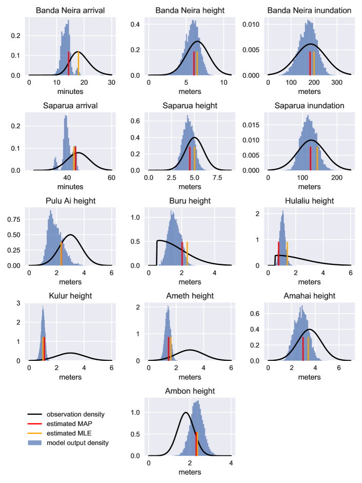
Figure 7: Model output compared to observation distributions. The blue histograms represent the forward model outputs corresponding to the posterior distribution. The black curves are the observation densities assigned to each observation. The model outputs corresponding to the estimated maximum a posteriori (MAP) point and maximum likelihood estimate (MLE) are marked with red and orange lines, respectively.

5.3 Error Bounds and Sensitivity

Given the necessarily uncertain process of interpreting textual records as probability distributions, it would be natural to question how sensitive the results are to different choices of the observation distribution. To allay some of these concerns, in this section we estimate upper and lower bounds on the potential error in the posterior distribution due to the choice of likelihood. That is, whereas Section 5.2 presents estimates of and uncertainty in the earthquake parameters as a result of the uncertain data (historical accounts), here we investigate the sensitivity of those estimates with respect to changes in our likelihood model in particular changes in the observational probability distributions.

To do so, we use three theoretical results from [13], which provides various bounds on estimates derived from probability distributions as those distributions are perturbed. First, we use a second order estimate for the relative entropy (Kullback–Leibler divergence) $\mathcal{R}$ between a distribution $P^{\theta}$ and its perturbation $P^{\theta+v}$ (see [13, Equation 2.35]):

$$\mathcal{R}(P^{\theta+v}||P^{\theta})=\frac{1}{2}v^{T}\mathcal{I}\left(P^{\theta}\right)v+\mathcal{O}\left(|v|^{3}\right),$$ (8)

where $\mathcal{I}$ is the Fisher information matrix (FIM). From [13] we also use upper and lower bounds for the difference in expected value of an observable between the original and perturbed distributions; these bounds are shown below in (9). Finally, from [13] we use bounds on the sensitivity of estimates of observables due to perturbations in a distribution; this relationship is shown in (10). Throughout, expected values are approximated using Monte Carlo integration on the posterior samples described in Section 5.

To define the perturbations that we consider, we begin by parameterizing the observation distributions $p_{l}$ shown in Figure 3. To do so, we fix the structure of the choice of $p_{l}$ – e.g., if the distribution is normal in Figure 3 we continue to use a normal distribution – and let the parameters, denoted by $\theta$, be the parameters characterizing that distribution, e.g., the mean and variance for a normal distribution. A full parameterization of the posterior measure in this way requires 29 parameters; a full list is shown in Table 2.

Table 2 also shows our first set of sensitivity estimates. First, for each $\theta$ parameter we list the associated Fisher information (the diagonal element of the FIM). The definition of the FIM and a derivation for the posterior (1) are given in Appendix B. Because the differences in Fisher information for absolute changes in parameter values are largely driven by units (e.g., meters for wave height vs. minutes for arrival time), the Fisher information values presented in the table are computed for the relative change in each parameter value. Second, we present the relative entropy (Kullback–Leibler divergence) $\mathcal{R}$ associated with a $10\%$ shift in each parameter computed from (8). That is, for $P^{\theta}$ we use the original posterior distribution shown in Section 5.2; for the perturbation $v$ for the $i^{\text{th}}$ row in the table we set $v_{i}=0.1\theta_{i}$ and $v_{j}=0,j\neq i$. Finally, the last column in Table 2 lists the first singular vector of the FIM, which is the combination of perturbations of the observation parameters that produce the largest relative entropy – effectively the “worst-case” perturbation. The results show that the most sensitive parameters of the observation distributions are the means of the arrival times at Saparua and Banda Neira. These two parameters seem to be the most sensitive because they are the only two arrival time measurements, so their values seem to provide the most “triangulation” information about earthquake location and magnitude.

Table 2: Observation distribution parameters, associated Fisher Information values, relative entropy according to (8) associated with a 10% relative perturbation, and the first (most sensitive) singular vector of the Fisher information matrix.

Name	Observation	Distribution	Parameter ($\theta$)	Value	FI	$\mathcal{R}~{}10\%$	Sing. Vec.
Pulu Ai	height	normal	mean	3	5.934	0.030	-0.151
Pulu Ai	height	normal	std	0.8	2.505	0.013	0.087
Ambon	height	normal	mean	1.8	12.370	0.062	0.364
Ambon	height	normal	std	0.4	5.220	0.026	0.216
Banda Neira	arrival	skewnorm	mean	15	14.082	0.070	0.447
Banda Neira	arrival	skewnorm	std	5	1.950	0.010	-0.148
Banda Neira	arrival	skewnorm	a	2	1.339	0.007	0.132
Banda Neira	height	normal	mean	6.5	7.525	0.038	-0.014
Banda Neira	height	normal	std	1.5	0.884	0.004	-0.006
Banda Neira	inundation	normal	mean	185	2.663	0.013	-0.010
Banda Neira	inundation	normal	std	65	0.272	0.001	-0.006
Buru	height	chi	mu	0.5	0.006	0.000	0.009
Buru	height	chi	sigma	1.5	0.122	0.001	0.035
Buru	height	chi	dof	1.01	0.142	0.001	0.040
Hulaliu	height	chi	mu	0.5	0.001	0.000	0.000
Hulaliu	height	chi	sigma	2	0.003	0.000	-0.000
Hulaliu	height	chi	dof	1.01	0.185	0.001	0.002
Saparua	arrival	normal	mean	45	19.264	0.096	0.716
Saparua	arrival	normal	std	5	1.280	0.006	-0.163
Saparua	height	normal	mean	5	9.085	0.045	0.009
Saparua	height	normal	std	1	0.869	0.004	-0.005
Saparua	inundation	normal	mean	125	2.905	0.015	0.005
Saparua	inundation	normal	std	40	0.178	0.001	-0.003
Kulur	height	normal	mean	3	0.199	0.001	0.038
Kulur	height	normal	std	1	0.362	0.002	-0.050
Ameth	height	normal	mean	3	0.351	0.002	0.043
Ameth	height	normal	std	1	0.409	0.002	-0.046
Amahai	height	normal	mean	3.5	4.107	0.021	0.014
Amahai	height	normal	std	1	0.784	0.004	-0.001

To gauge the effect of such perturbations on estimates of earthquake characteristics, we use the following bound on the expected value of an observable $f$ with respect to model $Q$ in terms of the values of $f$ according to model $P$ from [13, Equation 2.11]:

$$\sup_{c>0} \left(-\frac{1}{c}\log\mathbb{E}_{P}\left[e^{-c(f-\mathbb{E}_{P}[f])}\right]-\frac{1}{c}\mathcal{R}(Q||P)\right)$$ (9)

$$\qquad\leq\mathbb{E}_{Q}[f]-\mathbb{E}_{P}[f]\leq\inf_{c>0}\left(\frac{1}{c}\log\mathbb{E}_{P}\left[e^{c(f-\mathbb{E}_{P}[f])}\right]+\frac{1}{c}\mathcal{R}(Q||P)\right).$$

Here $\mathbb{E}_{P}$ and $\mathbb{E}_{Q}$ are the expected values according to $P$ and $Q$, respectively, and $Q$ is assumed to be absolutely continuous with respect to $P$ (that is, $P(A)=0\implies Q(A)=0$ for any event $A$). By letting $P$ be the posterior measure, we can estimate the uncertainty in observables with respect to other similar measures/models $Q$.

The expressions inside the $\sup$ and $\inf$ in (9) can be differentiated to find the value of $c$ that provides the optimal bound for a given value of $\mathcal{R}(Q||P)$. When $f$ is bounded, the equations also give a global upper and lower bound $\mathbb{E}_{Q}[f]$. Details of these derivations and a plot of the resulting bounds in terms of $\mathcal{R}(Q||P)$ are reserved for Appendix C.

By combining these bounds with (8) (by setting $Q=P^{\theta+v}$), we can estimate bounds on our estimates of earthquake parameters for perturbations of observation distributions. To model the worst-case scenario, we assume a perturbation in the direction of the first singular vector of $\mathcal{I}$ (the last column in Table 2); this perturbation, which is primarily made up of changes to the arrival times in Banda Neira and Saparua, will produce the largest sensitivity for a given norm $\|v\|_{2}$. The resulting bounds are shown in Figure 8.

We see that even for relatively large perturbations, we get relatively narrow bounds on posterior estimates. For example, even with a 25% perturbation in the most sensitive direction, the expected value of magnitude according to the perturbed posterior distribution would be between 8.7 and 9.0 – a very large earthquake in any case. These narrow bounds are an encouraging sign that the posterior measure is robust to small changes in the choice of observation distributions – i.e., that our Bayesian approach is quite robust to the way that we formulated our likelihood function. (One caveat: As the size of the perturbation grows, the approximation in (8) may break down. In this case, we refer the reader to Figure 10, where the $x$-axis is in terms of relative entropy taken directly from (9).)

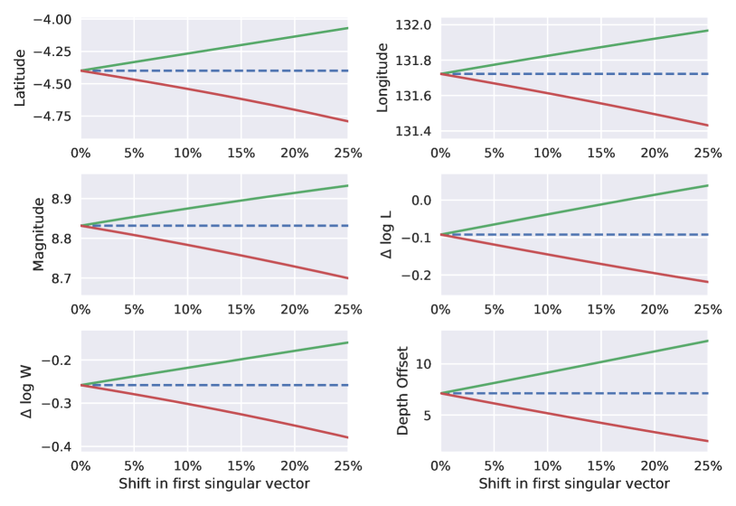
Figure 8: Bounds on mean parameter values in terms of relative perturbation in the first singular vector of the Fisher information matrix (see the last column of Table 2). Upper and lower bounds are in green and red, respectively. The posterior mean is in blue.

Finally, [13, Equation 2.39] gives bounds on the sensitivity of estimates of observables due to changes in the likelihood (perturbations in $\theta$):

$$\left|S_{f,v}\left(P^{\theta}\right)\right|\leq\sqrt{\mathbb{V}_{P^{\theta}}(f)}\sqrt{v^{T}\mathcal{I}\left(P^{\theta}\right)v}.$$ (10)

Here $f$ is an observable, which we will consider to be our six earthquake parameters, $\mathbb{V}$ denotes variance, and the sensitivity bound $S_{f,v}$ is the approximate derivative of $\mathbb{E}_{P^{\theta}}[f]$ with respect to perturbation of $\theta$ in the direction of $v$. Equation 10 shows that the greatest sensitivity will occur when the perturbation $v$ heavily weights likelihood parameters $\theta$ that most affect the posterior (the second term) and when earthquake parameters $f$ have the most uncertainty in the posterior (the first term). To estimate the worst-case scenario, we again assume here that the perturbation $v$ is along the first singular vector of $\mathcal{I}$. The sensitivity bounds associated with a $10\%$ relative perturbation in this direction are presented in Table 3. Among earthquake parameters, the greatest sensitivities were associated with depth offset because, as shown in Figure 5, it had the widest distribution according to the posterior measure. This also indicates that depth offset is the least certain inferred parameter for this earthquake, as opposed to the small sensitivity for the magnitude and $\Delta\log L$ and $\Delta\log W$ which indicate that the inferred values of these three parameters representing the size of the earthquake are quite certain.

Table 3: Posterior variance and sensitivity bound according to (10) by earthquake parameter. Sensitivity bound is for relative perturbation of $10\%$ in the direction of the first (worst-case) singular vector of the Fisher Information matrix.

Parameter	Variance	Sensitivity Bound
Latitude	0.066	0.135
Longitude	0.040	0.105
Magnitude	0.008	0.046
$\Delta$ log L	0.011	0.054
$\Delta$ log W	0.006	0.041
Depth Offset	14.483	1.997

6 Discussion

Methodology. The results for the 1852 Banda Arc earthquake and tsunami show the promise of the described methodology: even though the historical accounts of the tsunami are textual in nature and therefore individually prone to much uncertainty, it nevertheless appears that taken together they can be used to determine key characteristics of the causal earthquake. The approach is similar to the “ad hoc” approach described in Section 2.2, but with a more reproducible and rigorous set of assumptions, a more comprehensive coverage of possible events via automation, and a more clear characterization of uncertainty on the results. The strategy outlined in Section 3.1 can readily be applied to any number of historical seismic events, but also any other problem of inverting from textual accounts similar in nature to those described in Section 2 or any other historical or other data that is similarly “small” – sparse and riddled with uncertainty, so long as a reasonably believable forward model is available with parameters on which we can formulate a suitable prior distribution.

Software Package. To fully document the methodology and ease application to additional historical seismic events, the approach described in this paper has been packaged into a Python library called tsunamibayes. The package is open-source and available on GitHub: https://github.com/jpw37/tsunamibayes. Since each historical scenario may have a unique interpretation as a Bayesian inference problem – e.g., different parameters/priors, modified/generalized forward model, additional types of observations – the core code of the module does not assume particular features, but rather provides a suite of tools that can be recombined or modified to suit the needs of the user. A further description of the software package is available in [53, Chapter 7]. Datasets for this research are available in these in-text data citation references: [67].

Future Work. Any reconstruction of historical events is going to beg the question “How do we know if the result is right?” In particular, for the Bayesian approach described here, there is inherent uncertainty in the likelihood distributions stemming from the historical record. One avenue of future research will therefore be to supplement the theoretical results presented in Section 5.3 with a numerical study of the robustness of the posterior to changing interpretations of the likelihood. A second effort will validate the approach by using it to “reconstruct” a modern event for which the truth is known from instrumental data and plentiful newspaper and historical accounts are available. Finally, there are a number of methodological refinements, e.g., to the sampling approach, that might yield faster or better resolved results, and there are dozens of other historical earthquakes of interest in the Wichmann catalog ready for reconstruction that will improve modern understanding of seismic risk.

Appendix A Plot of Gelman-Rubin Diagnostic

In this appendix we show a plot of the Gelman-Rubin diagnostic $\hat{R}$ for MCMC convergence; see the discussion in Section 5.1.

Appendix B Derivation of the Fisher Information Matrix

In this appendix we derive the Fisher Information Matrix (FIM) $\mathcal{I}$ associated with a parameterization of the posterior measure given in (1). The FIM associated with parameter $\theta$ is given by

$$\mathcal{I}(P^{(\theta)})=\int\nabla_{\theta}\log p^{(\theta)}(x)\left(\nabla_{\theta}\log p^{(\theta)}(x)\right)^{T}P^{(\theta)}(dx)$$ (11)

where $P^{(\theta)}$ is the posterior measure and $p^{(\theta)}$ its associated density given by (see (1) and (5))

$$p_{post}^{(\theta)}(x)dx=\frac{1}{Z^{(\theta)}}p_{0}^{(\theta)}(x)p_{l}^{(\theta)}\left(\mathcal{G}(x)\right)dx.$$

Since the focus of this paper is on modeling of historical observations via observation distributions, we will focus on the case where $\theta$ describes the observation distributions. In this case, we have

$$\mathcal{I}_{ij}(P^{(\theta)})=\mathrm{Cov}_{P^{(\theta)}}\left[\frac{\partial}{\partial\theta_{i}}\Phi^{(\theta)},\frac{\partial}{\partial\theta_{j}}\Phi^{(\theta)}\right]$$

where $\mathrm{Cov}_{P^{(\theta)}}$ is the covariance according to the posterior and $\Phi^{(\theta)}$ is the negative log-likelihood given by

$$\Phi^{(\theta)}(x) :=-\log p_{l}^{(\theta)}\left(\mathcal{G}(x)\right).$$

Thus, to compute the FIM, we compute the derivative of $\Phi^{(\theta)}$ with respect to each observation parameter (the “score”) and then compute the covariance of each pair of scores, which we approximate using the observations associated with the approximate posterior samples generated as described in Section 5. Since the individual distributions making up $p_{l}$ are assumed to be independent as described in Section 4.3, the derivatives can be computed separately for each observation distribution. We now consider each type of observation distribution listed in Table 2.

Normal Distribution

For a normal distribution with mean $\mu$ and standard deviation $\sigma$, we have

$$\Phi^{(\theta)}(x)=\frac{1}{2\sigma^{2}}\left[\mathcal{G}(x)-\mu\right]^{2}+\ln\sigma+\frac{1}{2}\ln(2\pi)$$

Then the derivatives with respect to parameters $\mu$ and $\sigma$ are given by:

$$\frac{\partial}{\partial\mu}\Phi^{(\theta)}(x) =-\frac{1}{\sigma^{2}}\left[\mathcal{G}(x)-\mu\right]$$

$$\frac{\partial}{\partial\sigma}\Phi^{(\theta)}(x) =-\frac{1}{\sigma^{3}}\left[\mathcal{G}(x)-\mu\right]^{2}+\frac{1}{\sigma}.$$

Skew-Norm Distribution

For a skew-normal distribution with location $\mu$, scale $\sigma$, and skew $a$, we have

$$\Phi(x) =\frac{1}{2}\tilde{x}(x)^{2}+\ln\sigma+\frac{1}{2}\ln(2\pi)-\ln\left[1+\text{erf}\left(z(x)\right)\right]$$

where erf is the error function and $\tilde{x},z$ are given by

$$\tilde{x}(x) :=\frac{\mathcal{G}(x)-\mu}{\sigma}\quad\text{and}\quad z(x):=\frac{a\tilde{x}(x)}{\sqrt{2}}.$$

Then the derivative with respect to $z$ and $\tilde{x}$ are given by

$$\frac{\partial}{\partial z}\Phi(x) =-\frac{2}{\sqrt{\pi}}\frac{e^{-z(x)^{2}}}{1+\text{erf}\left(z(x)\right)}$$

$$\frac{\partial}{\partial\tilde{x}}\Phi(x) =\frac{\partial}{\partial\tilde{x}}\Phi(x)+\frac{\partial\Phi}{\partial z}(x)\frac{\partial z}{\partial\tilde{x}}(x)=\tilde{x}(x)-\sqrt{\frac{2}{\pi}}a\frac{e^{-z(x)^{2}}}{1+\text{erf}\left(z(x)\right)},$$

so that the derivatives with respect to parameters $a$, $\mu$, and $\sigma$ are

$$\frac{\partial}{\partial a}\Phi(x) =\frac{\partial\Phi}{\partial z}(x)\frac{\partial z}{\partial a}(x)=-\sqrt{\frac{2}{\pi}}\tilde{x}(x)\frac{e^{-z(x)^{2}}}{1+\text{erf}\left(z(x)\right)}$$

$$\frac{\partial}{\partial\mu}\Phi(x) =\frac{\partial\Phi}{\partial\tilde{x}}(x)\frac{\partial\tilde{x}}{\partial\mu}(x)=-\frac{1}{\sigma}\left[\tilde{x}(x)-\sqrt{\frac{2}{\pi}}a\frac{e^{-z(x)^{2}}}{1+\text{erf}\left(z(x)\right)}\right]$$

$$\frac{\partial}{\partial\sigma}\Phi(x) =\frac{\partial}{\partial\sigma}\Phi(x)+\frac{\partial\Phi}{\partial\tilde{x}}(x)\frac{\partial\tilde{x}}{\partial\sigma}(x)=\frac{1}{\sigma}\left[1-\tilde{x}(x)^{2}+\frac{2z(x)}{\sqrt{\pi}}\frac{e^{-z(x)^{2}}}{1+\text{erf}\left(z(x)\right)}\right].$$

Chi Distribution

For the Chi distribution with location $\mu$, scale $\sigma$, and degrees of freedom $k$, we have

$$\Phi(x) =\frac{1}{2}\tilde{x}(x)^{2}+\ln\sigma+\left(\frac{k}{2}-1\right)\ln 2+\ln\Gamma\left(k/2\right)-(k-1)\ln\tilde{x}(x),$$

where $\Gamma$ is the gamma function and $\tilde{x}$ is given by

$$\tilde{x}(x):=\frac{\mathcal{G}_{i}(x)-\mu}{\sigma}.$$

The derivative with respect to $\tilde{x}$ is given by

$$\frac{\partial\Phi}{\partial\tilde{x}}(x) =\tilde{x}(x)-(k-1)\tilde{x}(x)^{-1}.$$

Then the derivatives with respect to parameters $\mu$, $\sigma$, and $k$ are given by

$$\frac{\partial\Phi}{\partial\mu}(x) =\frac{\partial\Phi}{\partial\tilde{x}}\frac{\partial\tilde{x}}{\partial\mu}=-\frac{1}{\sigma}\left(\tilde{x}(x)-(k-1)\tilde{x}(x)^{-1}\right)$$

$$\frac{\partial\Phi}{\partial\sigma}(x) =\frac{\partial\Phi}{\partial\sigma}+\frac{\partial\Phi}{\partial\tilde{x}}\frac{\partial\tilde{x}}{\partial\sigma}=-\frac{1}{\sigma}\left(\tilde{x}(x)^{2}-k\right).$$

$$\frac{\partial\Phi}{\partial k}(x) =\frac{1}{2}\ln 2+\frac{1}{2}\psi\left(k/2\right)-\ln\tilde{x}(x)$$

where $\psi$ is the digamma function.

Appendix C Derivation of Bounds in Terms of Relative Entropy

In this section, we derive from (9) more explicit bounds on $\mathbb{E}_{Q}[f]$ – first in terms of $\mathcal{R}(Q||P)$ and then independent of $\mathcal{R}(Q||P)$. These bounds were used to generate Figure 10, below, which shows the bounds on estimates of parameters of the 1852 Banda Arc earthquake in terms of $\mathcal{R}(Q||P)$. These bounds were then combined with the estimate from (8) to produce the plots in terms of relative parameter value changes shown in Figure 8.

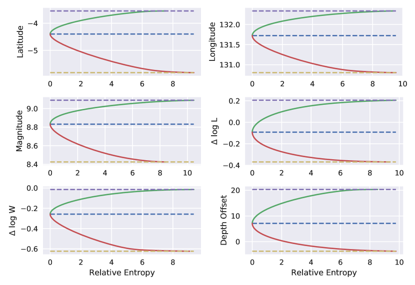
Figure 10: Bounds on mean parameter values by relative entropy from computed posterior. Upper and lower bounds are in green and red, respectively. The posterior mean is in blue and the estimated uniform upper and lower bounds are in purple and yellow, respectively.

C.1 Optimal Bound for a Given $\mathcal{R}(Q||P)$

Here we derive a relationship between the relative entropy $\mathcal{R}(Q||P)$ and the $c<\infty$ for which the bounds given by (9) are achieved. Here, we assume that such a $c$ exists; the case where the supremum/infimum are achieved as $c\to\infty$ is discussed in the next subsection. Denoting $\tilde{f}=f-\mathbb{E}_{P}[f]$ and differentiating the right hand side of (9) with respect to $c$ and setting equal to zero yields that the infimum of the upper bound is achieved when $c$ satisfies

$$\mathcal{R}(Q||P) =c\frac{\mathbb{E}_{P}\left[\tilde{f}e^{c\tilde{f}}\right]}{\mathbb{E}_{P}\left[e^{c\tilde{f}}\right]}-\log\mathbb{E}_{P}\left[e^{c\tilde{f}}\right]=c\frac{E_{2}(f,c)}{E_{1}(f,c)}-\log E_{1}(f,c)$$ (12)

and similarly for the lower bound $c$ must satisfy

$$\mathcal{R}(Q||P) =-c\frac{\mathbb{E}_{P}\left[\tilde{f}e^{-c\tilde{f}}\right]}{\mathbb{E}_{P}\left[e^{-c\tilde{f}}\right]}-\log\mathbb{E}_{P}\left[e^{-c\tilde{f}}\right]=-c\frac{E_{2}(f,-c)}{E_{1}(f,-c)}-\log E_{1}(f,-c)$$ (13)

where to simplify notation we have defined

$$E_{1}(f,c)=\mathbb{E}_{P}\left[e^{c\tilde{f}}\right]\quad\text{and}\quad E_{2}(f,c)=\mathbb{E}_{P}\left[\tilde{f}e^{c\tilde{f}}\right].$$

Denoting the $c$ achieving these upper and lower bounds by $c_{+}$ and $c_{-}$, respectively, and plugging these values back into (9) yields the bounds

$$\frac{E_{2}(f,-c_{-})}{E_{1}(f,-c_{-})}\leq\mathbb{E}_{Q}[f]-\mathbb{E}_{P}[f]\leq\frac{E_{2}(f,c_{+})}{E_{1}(f,c_{+})}.$$ (14)

It is not clear how to invert (12) and (13) to find the optimal $c$ for a given $\mathcal{R}(Q||P)$, so to generate Figure 10 (and, by extension, Figure 8) we generate a list of $c$ values, plug them into (12) to find the $\mathcal{R}(Q||P)$ for which they achieve the optimal upper bound and into (14) to compute the associated upper bounds (analogously for the lower bounds), and plot those values against each other.

C.2 Bounds Independent of $\mathcal{R}(Q||P)$

In this section, we consider the case where the bounds in (9) are achieved as $c\to\infty$, i.e., are independent of $\mathcal{R}(Q||P)$. From (9), we have for any $Q\ll P$

$$\mathbb{E}_{Q}[f]-\mathbb{E}_{P}[f] \leq\sup_{c>0}\frac{1}{c}\log\mathbb{E}_{P}\left[e^{c(f-\mathbb{E}_{P}[f])}\right]+\frac{1}{c}\mathcal{R}(Q||P).$$

Then clearly if

$$U:=\lim_{c\to\infty}\frac{1}{c}\log\mathbb{E}_{P}\left[e^{c(f-\mathbb{E}_{P}[f])}\right]<\infty,$$ (15)

then for any $Q\ll P$ we have

$$\mathbb{E}_{Q}[f]-\mathbb{E}_{P}[f] \leq\lim_{c\to\infty}\left\{\frac{1}{c}\log\mathbb{E}_{P}\left[e^{c(f-\mathbb{E}_{P}[f])}\right]+\frac{1}{c}\mathcal{R}(Q||P)\right\}=U.$$

Finally, we note that since the logarithm and exponential are continuous, we have

$$U =\lim_{c\to\infty}\frac{1}{c}\log\mathbb{E}_{P}\left[e^{c(f-\mathbb{E}_{P}[f])}\right]=\lim_{c\to\infty}\log\left(\mathbb{E}_{P}\left[e^{c(f-\mathbb{E}_{P}[f])}\right]\right)^{1/c}$$

$$=\log\lim_{c\to\infty}\left(\mathbb{E}_{P}\left[e^{c(f-\mathbb{E}_{P}[f])}\right]\right)^{1/c}=\log\left\|e^{f-\mathbb{E}_{P}[f]}\right\|_{\infty}=\mathrm{sup\,ess}_{P}[f]-\mathbb{E}_{P}[f]$$

An analogous relationship will hold for the lower bound. Thus if $f$ is an essentially bounded random variable according to $P$, we have the following bound for any $Q\ll P$:

$$\mathrm{inf\,ess}_{P}[f]\leq\mathbb{E}_{Q}[f]\leq\mathrm{sup\,ess}_{P}[f].$$

Funding Information

JAK was partially supported by NSF Grant DMS-2108791. JPW was partially supported by the Simons Foundation travel grant under 586788. NEGH was partially supported by NSF Grants DMS-1816551 and DMS-2108790. AJH was supported by NIH grant K25 AI153816, NSF grant DMS 2152774 and a generous gift from the Karen Toffler Charitable Trust. JPW and RH would like to thank the Office of Research and Creative Activities at BYU for supporting several of the students’ efforts on this project through a Mentoring Environment Grant, as well as generous support from the College of Physical and Mathematical Sciences and the Mathematics and Geology Departments. We also acknowledge the visionary support of Geoscientists Without Borders.

Justin Krometis
National Security Institute
Virginia Tech
Web: https://krometis.github.io/
Email: jkrometis@vt.edu

Jared P. Whitehead
Department of Mathematics
Brigham Young University
Email: whitehead@mathematics.byu.edu

Ron Harris
Department of Geology
Brigham Young University
Email: rharris@byu.edu

Hayden Ringer
Department of Mathematics
Virginia Tech
Web: https://sites.google.com/view/hringer/home
Email: hringer@vt.edu

Nathan E. Glatt-Holtz
Department of Mathematics
Tulane University
Web: http://www.math.tulane.edu/~negh/
Email: negh@tulane.edu

Andrew Holbrook
Department of Biostatistics
UCLA
Web: https://andrewjholbrook.github.io/
Email: aholbroo@g.ucla.edu

References

- [1] James H Albert and Siddhartha Chib. Bayesian analysis of binary and polychotomous response data. Journal of the American statistical Association, 88(422):669–679, 1993.
- [2] B. Barber. Tsunami relief. Technical report, US Agency for International Development, 2005.
- [3] M. J. Berger, D. L. George, R. J. LeVeque, and K. T. Mandli. The GeoClaw software for depth-averaged flows with adaptive refinement. Advances in Water Resources, 34(9):1195–1206, 2011.
- [4] P. Bergsma. Aardbevingen in den indischen archipel gedurende het jaar 1867. Natuurkundig Tijdschrift Voor Nederlandsch-Indië, 30:478–485, 1868.
- [5] Stephen P. Brooks and Andrew Gelman. General Methods for Monitoring Convergence of Iterative Simulations. Journal of Computational and Graphical Statistics, 7(4):434–455, December 1998.
- [6] E Bryant, Grant Walsh, and Dallas Abbott. Cosmogenic mega-tsunami in the Australia region: are they supported by Aboriginal and Maori legends? Geological Society, London, Special Publications, 273(1):203–214, 2007.
- [7] Tan Bui-Thanh, Omar Ghattas, James Martin, and Georg Stadler. A computational framework for infinite-dimensional bayesian inverse problems part i: The linearized case, with application to global seismic inversion. SIAM Journal on Scientific Computing, 35(6):A2494–A2523, 2013.
- [8] George Casella and Roger L Berger. Statistical inference. Cengage Learning, 2021.
- [9] P. R. Cummins, I. R. Pranantyo, J. M. Pownall, J. D. Griffin, I. Meilano, and S. Zhao. Earthquakes and tsunamis caused by low-angle normal faulting in the banda sea, indonesia. Nature Geoscience, 13(4):312–318, 2020.
- [10] M. Dashti and A. M. Stuart. The Bayesian approach to inverse problems. Handbook of Uncertainty Quantification, pages 311–428, 2017.
- [11] A Molina del Villar. 19th century earthquakes in mexico: Three cases, three comparative studies. Annals of Geophysics, 47(2-3), 2004.
- [12] Arnaud Doucet, Nando De Freitas, and Neil Gordon. Sequential Monte Carlo methods in practice. Springer, 2001.
- [13] P. Dupuis, M. A. Katsoulakis, Y. Pantazis, and P. Plechác. Path-space information bounds for uncertainty quantification and sensitivity analysis of stochastic dynamics. SIAM/ASA Journal on Uncertainty Quantification, 4(1):80–111, 2016.
- [14] Ronald A Fisher. On the mathematical foundations of theoretical statistics. Philosophical transactions of the Royal Society of London. Series A, containing papers of a mathematical or physical character, 222(594-604):309–368, 1922.
- [15] T. L. Fisher and R. A. Harris. Reconstruction of 1852 Banda Arc megathrust earthquake and tsunami. Natural Hazards, 83(1):667–689, 2016.
- [16] M. K. Gagan, S. M. Sosdian, H. Scott-Gagan, K. Sieh, W. S. Hantoro, D. H. Natawidjaja, R. W. Briggs, B. W. Suwargadi, and H. Rifai. Coral 13c/12c records of vertical seafloor displacement during megathrust earthquakes west of sumatra. Earth and Planetary Science Letters, 432:461–471, 2015.
- [17] A. Gelman, J. B. Carlin, H. S. Stern, and D. B. Rubin. Bayesian data analysis, volume 2. Taylor & Francis, 2014.
- [18] A. Gelman, D. B. Rubin, et al. Inference from iterative simulation using multiple sequences. Statistical Science, 7(4):457–472, 1992.
- [19] R. Ghose and K. Oike. Characteristics of seismicity distribution along the sunda arc: some new observations. 1988.
- [20] Loïc Giraldi, Olivier P Le Maître, Kyle T Mandli, Clint N Dawson, Ibrahim Hoteit, and Omar M Knio. Bayesian inference of earthquake parameters from buoy data using a polynomial chaos-based surrogate. Computational Geosciences, 21(4):683–699, 2017.
- [21] C. Goldfinger, C. H. Nelson, J. E. Johnson, and Shipboard Scientific Party. Holocene earthquake records from the cascadia subduction zone and northern san andreas fault based on precise dating of offshore turbidites. Annual Review of Earth and Planetary Sciences, 31(1):555–577, 2003.
- [22] F. I. González, R. J. LeVeque, P. Chamberlain, B. Hirai, J. Varkovitzky, and D. L. George. Validation of the geoclaw model. In NTHMP MMS Tsunami Inundation Model Validation Workshop. GeoClaw Tsunami Modeling Group, 2011.
- [23] J. Griffin, N. Nguyen, P. Cummins, and A. Cipta. Historical Earthquakes of the Eastern Sunda Arc: Source Mechanisms and Intensity-Based Testing of Indonesia’s National Seismic Hazard Assessment. Bulletin of the Seismological Society of America, 109, 12 2018.
- [24] R. A. Harris. Who’s Next? Assessing vulnerability to geophysical hazards in densely populated regions of Indonesia. Bridges, Fall:14–17, 2002.
- [25] R. A. Harris, K. Donaldson, and C. Prasetyadi. Geophysical disaster mitigation in indonesia using gis. Buletin Teknologi Mineral, 5:2–10, 1997.
- [26] R. A. Harris and J. Major. Waves of destruction in the East Indies: the Wichmann catalogue of earthquakes and tsunami in the Indonesian region from 1538 to 1877. Geological Society, London, Special Publications, 441:SP441–2, 2016.
- [27] G. P. Hayes, G. L. Moore, D. E. Portner, M. Hearne, H. Flamme, M. Furtney, and G. M. Smoczyk. Slab2, a comprehensive subduction zone geometry model. Science, 362(6410):58–61, 2018. Slab2 GitHub: https://github.com/usgs/slab2, data download: https://www.sciencebase.gov/catalog/item/5aa1b00ee4b0b1c392e86467.
- [28] Andrew J. Holbrook, Xiang Ji, and Marc A. Suchard. Bayesian mitigation of spatial coarsening for a Hawkes model applied to gunfire, wildfire and viral contagion. The Annals of Applied Statistics, 16(1):573–595, March 2022.
- [29] Kruawun Jankaew, Brian F Atwater, Yuki Sawai, Montri Choowong, Thasinee Charoentitirat, Maria E Martin, and Amy Prendergast. Medieval forewarning of the 2004 Indian Ocean tsunami in Thailand. Nature, 455(7217):1228, 2008.
- [30] J. Kaipio and E. Somersalo. Statistical and computational inverse problems, volume 160 of Applied Mathematical Sciences. Springer Science & Business Media, 2005.
- [31] K. Kay. Devastating 2004 tsunami cleared the way for better infrastructure in indonesia? Public Broadcasting System, 2014.
- [32] R. L. Kovach and R. L. Kovach. Early earthquakes of the Americas. Cambridge University Press, 2004.
- [33] R. J. LeVeque and D. L. George. High-resolution finite volume methods for the shallow water equations with bathymetry and dry states. In Advanced numerical models for simulating tsunami waves and runup, pages 43–73. World Scientific, 2008.
- [34] R. J. LeVeque, D. L. George, and M. J. Berger. Tsunami modelling with adaptively refined finite volume methods. Acta Numerica, 20:211–289, 2011.
- [35] Z. Y. C. Liu and R. A. Harris. Discovery of possible mega-thrust earthquake along the Seram Trough from records of 1629 tsunami in eastern Indonesian region. Natural Hazards, 72:1311–1328, 2014.
- [36] James Martin, Lucas C Wilcox, Carsten Burstedde, and Omar Ghattas. A stochastic newton mcmc method for large-scale statistical inverse problems with application to seismic inversion. SIAM Journal on Scientific Computing, 34(3):A1460–A1487, 2012.
- [37] S. S. Martin, L. Li, E. A. Okal, J. Morin, A. E. G. Tetteroo, A. D. Switzer, and K. E. Sieh. Reassessment of the 1907 Sumatra ”Tsunami Earthquake” Based on Macroseismic, Seismological, and Tsunami Observations, and Modeling. Pure and Applied Geophysics, 2019.
- [38] A. J. Meltzner, K. Sieh, H.-W. Chiang, C.-C. Shen, B. W. Suwargadi, D. H. Natawidjaja, B. E. Philibosian, R. W. Briggs, and J. Galetzka. Coral evidence for earthquake recurrence and an AD 1390–1455 cluster at the south end of the 2004 Aceh–Andaman rupture. Journal of Geophysical Research: Solid Earth, 115(B10), 2010.
- [39] K Minoura, F Imamura, D Sugawara, Y Kono, and T Iwashita. The 869 jogan tsunami deposit and recurrence interval of large-scale tsunami on the pacific coast of northeast japan. Journal of Natural Disaster Science, 23(2):83–88, 2001.
- [40] K. Monecke, W. Finger, D. Klarer, W. Kongko, B. G. McAdoo, A. L. Moore, and S. U. Sudrajat. A 1,000-year sediment record of tsunami recurrence in northern Sumatra. Nature, 455(7217):1232, 2008.
- [41] R. M. W. Musson. A provisional catalogue of historical earthquakes in indonesia. British Geological Survey, 2012.
- [42] R. M. W. Musson and M. J. Jiménez. Macroseismic estimation of earthquake parameters. NERIES project report, Module NA4, Deliverable D, 3, 2008.
- [43] KR Newcomb and WR McCann. Seismic history and seismotectonics of the sunda arc. Journal of Geophysical Research: Solid Earth, 92(B1):421–439, 1987.
- [44] KR Newcomb and WR McCann. Seismic history and seismotectonics of the Sunda Arc. Journal of Geophysical Research: Solid Earth, 92(B1):421–439, 1987.
- [45] Y. Okada. Surface deformation due to shear and tensile faults in a half-space. Bulletin of the seismological society of America, 75(4):1135–1154, 1985.
- [46] Emile A Okal and Dominique Reymond. The mechanism of great banda sea earthquake of 1 february 1938: applying the method of preliminary determination of focal mechanism to a historical event. earth and planetary science letters, 216(1-2):1–15, 2003.
- [47] B. Philibosian, K. Sieh, J.-P. Avouac, D. H. Natawidjaja, H.-W. Chiang, C.-C. Wu, C.-C. Shen, M. R. Daryono, H. Perfettini, B. W. Suwargadi, et al. Earthquake supercycles on the mentawai segment of the sunda megathrust in the seventeenth century and earlier. Journal of Geophysical Research: Solid Earth, 122(1):642–676, 2017.
- [48] I. R. Pranantyo and P. R. Cummins. The 1674 ambon tsunami: Extreme run-up caused by an earthquake-triggered landslide. Pure and Applied Geophysics, 177(3):1639–1657, 2020.
- [49] A. Reid. Historical evidence for major tsunamis in the java subduction zone. Asia Research Institute Working Paper Series, pages 1–9, 2012.
- [50] Anthony Reid. Two hitherto unknown Indonesian tsunamis of the seventeenth century: Probabilities and context. Journal of Southeast Asian Studies, 47(1):88–108, 2016.
- [51] C. G. C. Reinwardt. Reis naar het oostelijk gedeelte van den indischen archipel, in het jaar 1821. 1858.
- [52] Hayden Ringer, Jared P Whitehead, Justin Krometis, Ronald A Harris, Nathan Glatt-Holtz, Spencer Giddens, Claire Ashcraft, Garret Carver, Adam Robertson, McKay Harward, et al. Methodological reconstruction of historical seismic events from anecdotal accounts of destructive tsunamis: a case study for the great 1852 banda arc mega-thrust earthquake and tsunami. Journal of Geophysical Research, 2021.
- [53] Hayden J. Ringer. A method for reconstructing historical destructive earthquakes using bayesian inference. Master’s thesis, Brigham Young University, 2020.
- [54] C. M. Rubin, B. P. Horton, K. Sieh, J. E. Pilarczyk, P. Daly, N. Ismail, and A. C. Parnell. Highly variable recurrence of tsunamis in the 7,400 years before the 2004 indian ocean tsunami. Nature communications, 8:16019, 2017.
- [55] K. Sieh, D. H. Natawidjaja, A. J. Meltzner, C.-C. Shen, H. Cheng, K.-S. Li, B. W. Suwargadi, J. Galetzka, B. Philibosian, and R. L. Edwards. Earthquake supercycles inferred from sea-level changes recorded in the corals of west Sumatra. Science, 322(5908):1674–1678, 2008.
- [56] S. K. Singh, L. Astiz, and J. Havskov. Seismic gaps and recurrence periods of large earthquakes along the mexican subduction zone: a reexamination. Bulletin of the Seismological Society of America, 71(3):827–843, 1981.
- [57] SL Soloviev and Ch N Go. Catalog of tsunamis in western coast of the Pacific Ocean. Academy of Sciences, USSR, Izdat. Nauka, pages 1–130, 1974.
- [58] S. Stein, R. J. Geller, and M. Liu. Why earthquake hazard maps often fail and what to do about it. Tectonophysics, 562:1–25, 2012.
- [59] A. M. Stuart. Inverse problems: a Bayesian perspective. Acta Numerica, 19:451–559, 2010.
- [60] H. Sulaeman, R. A. Harris, P. Putra, S. Hall, I. Rafliana, and C. Prasetyadi. Megathrust Earthquakes Along The Java Trench: Discovery Of Possible Tsunami Deposits In The Lesser Sunda Islands, Indonesia. Geological Society of America Abstracts with Programs, 49(6), 2017.
- [61] Jacob Swart. Verhandelingen en Berigten Betrekkelijk het Zeewegen en de Zeevaartkunde (English: Treatises and Reports Related to the Seaways and Nautical Sciences). 13:257–274, 1853.
- [62] Martin A. Tanner and Wing Hung Wong. The Calculation of Posterior Distributions by Data Augmentation. Journal of the American Statistical Association, 82(398):528–540, June 1987.
- [63] A. Tarantola. Inverse Problem Theory and Methods for Model Parameter Estimation. SIAM, 2005.
- [64] UNISDR. Global assessment report on disaster risk reduction. United Nations International Strategy for Disaster Reduction Secretariat, 2009.
- [65] David A Van Dyk and Xiao-Li Meng. The art of data augmentation. Journal of Computational and Graphical Statistics, 10(1):1–50, 2001.
- [66] Donald L Wells and Kevin J Coppersmith. New empirical relationships among magnitude, rupture length, rupture width, rupture area, and surface displacement. Bulletin of the seismological Society of America, 84(4):974–1002, 1994.
- [67] Jared P. Whitehead. tsunamibayes: 1852 paper submission, October 2020.
- [68] A. Wichmann. The earthquakes of the Indian archipelago to 1857. Verhandl. Koninkl. Akad. van Wetenschappen, 2nd sec, 20(4):1–193, 1918.
- [69] A. Wichmann. The earthquakes of the Indian archipelago from 1858 to 1877. Verhandl. Koninkl. Akad. van Wetenschappen, 2nd sec, 22(5):1–209, 1922.
- [70] J. Zachariasen, K. Sieh, F. W. Taylor, R. L. Edwards, and W. S. Hantoro. Submergence and uplift associated with the giant 1833 sumatran subduction earthquake: Evidence from coral microatolls. Journal of Geophysical Research: Solid Earth, 104(B1):895–919, 1999.