Interaction effects in Graphene in a weak magnetic field

Abstract

A weak perpendicular magnetic field, $B$, breaks the chiral symmetry of each valley in the electron spectrum of graphene, preserving the overall chiral symmetry in the Brillouin zone. We explore the consequences of this symmetry breaking for the interaction effects in graphene. In particular, we demonstrate that the electron-electron interaction lifetime acquires an anomalous $B$-dependence. Also, the ballistic zero-bias anomaly, $\delta\nu(\omega)$, where $\omega$ is the energy measured from the Fermi level, emerges at a weak $B$ and has the form $\delta\nu(B)\sim B^{2}/\omega^{2}$. Temperature dependence of the magnetic-field corrections to the thermodynamic characteristics of graphene is also anomalous. We discuss experimental manifestations of the effects predicted. The microscopic origin of the $B$-field sensitivity is an extra phase acquired by the electron wave-function resulting from the chirality-induced pseudospin precession.

Introduction. Electron spectrum in graphene possesses a chiral (pseudo-spin) structureSemenoff (1984); Katsnelson et al. (2006). Two pseudospin projections are identified with two points, $K$ and $K^{\prime}$, of the Brillouin zone near which the spectrum is characterized by a massless Dirac dispersion. Numerous consequences of the Dirac spectrum of graphene for the disorder and interaction effects were established, see e.g. Refs. Altland, 2006; Aleiner and Efetov, 2006; Tse et al., 2008; Castro Neto et al., 2009; Das Sarma et al., 2011; Kotov et al., 2012; Semenoff, 2012; Nandkishore et al., 2012; Dutreix et al., 2019; Agarwal and Mishchenko, 2020; Maiti and Sedrakyan, 2019; Pack et al., 2020; Leeb et al., 2021; Sbierski et al., 2021; Guo et al., 2021; Bouaziz et al., 2021; Rostami and Cappelluti, 2021; Narozhny et al., 2021.

One distinctive feature of the graphene bandstructure is the absence of backscattering from the impurities. This feature is a consequence of orthogonality of the spinors corresponding to the wave vectors ${\bf k}$ and $-{\bf k}$. In turn, the absence of backscattering leads to the suppression of the oscillations of electron density (Friedel oscillationsFriedel (1952)) created by an impurity in graphene.Chen and Raikh (1999); Cheianov and Fal’ko (2006) In the ballistic regimeRudin et al. (1997); Zala et al. (2001a, b, c), electron scattering from individual impurities dressed by the Friedel oscillations is responsible for a zero-bias anomaly $\propto\ln\omega$ in conventional 2D electron gas. Here $\omega$ is the energy measured from the Fermi level and the condition $\omega\tau\gg 1$, where $\tau$ is the elastic scattering time, is implied. Fast decay of the Friedel oscillations suggests that zero-bias anomaly in graphene is absent.Nomura and MacDonald (2007); Cheianov and Fal’ko (2006) More detailed studyMariani et al. (2007) indicated that it is the Hartree correction which is absent in graphene, while the Fock correction, originating from the forward scattering, is still present.

In the absence of impurities, electron-electron interactions in 2D electron gas cause non-analytic correctionsGiuliani and Quinn (1982); Jungwirth and MacDonald (1996); Zheng and Das Sarma (1996); Chubukov and Maslov (2003) to the self-energy, $\Sigma(\omega)$. At low temperatures, $T\ll\omega$, the imaginary part of self-energy has the form $\tau_{ee}(\omega)^{-1}\sim(\omega^{2}/E_{F})\ln(E_{F}/\omega)$, where $E_{F}$ is the Fermi energy. Correspondingly, the real part of self-energy behaves as $\text{Re}\Sigma(\omega)\sim\omega^{2}\text{sgn}(\omega)$. At finite $T$, interactions cause a correction to the specific heatMisawa (1999); Coffey and Bedell (1993) $\delta C(T)\propto T^{2}$. Microscopically, the above corrections emerge in the random-phase approximation. Their derivation is so general that it is natural to expect that, in doped graphene, the interaction corrections have the same Fermi-liquid form.Das Sarma et al. (2007)

In the present letter, we identify the interaction effects specific to graphene. These effects emerge in the presence of a weak magnetic field. Their origin is the field-induced lifting of chiral symmetry in $K$ and $K^{\prime}$ valleys of graphene while preserving the overall symmetry. To capture these effects, one should go beyond the random-phase approximation.

With regard to ballistic zero-bias anomaly, lifting of the chiral symmetry in the field, $B$, gives rise to the contribution $\propto B^{2}/\omega^{2}$, which can be even stronger than the zero-field contribution.Mariani et al. (2007) A formal difference between the calculations of the ballistic zero-bias anomaly in electron gas with parabolic spectrum and in graphene is that the Green functions, which enter into the calculation, have a matrix structure in graphene. Without this matrix structure, the $B$-sensitive contributions to the tunnel conductance cancel out.

A natural energy scale imposed by the field, $B$, in graphene is $\omega_{0}=v_{F}/R_{L}$, where $R_{L}\propto B^{-1}$ is the Larmour radius. Quantization of the energy levels can be neglected for $\omega\gg\omega_{0}$. We show that the $B$-dependent correction to the thermodynamic characteristics of the clean graphene can be conveniently expressed in terms of $\omega_{0}$. Namely, the corrections to the imaginary and real parts of self-energy behave as $\text{Im}\left[\Sigma(\omega,B)-\Sigma(\omega,0)\right]\sim\omega_{0}^{2}E_{F}^{-1}\ln(\omega/T)$ and $\text{Re}\left[\Sigma(\omega,B)-\Sigma(\omega,0)\right]\sim\omega_{0}^{2}E_{F}^{-1}\text{sgn}(\omega)$, respectively. On the basis of these results we draw the consequences for observables. Namely, we show that the $B$-dependent correction to the specific heat is temperature-independent in a wide temperature interval.

Electrons in a weak magnetic field. The Hamiltonian of monolayer graphene which incorporates the $B$ field in the Landau gauge reads

$$\hat{H}_{B}=v_{F}\left[(p_{x}-eBy)\hat{\Sigma}_{x}+p_{y}\hat{\Sigma}_{y}\right].$$ (1)

Here $v_{F}$ is the Fermi velocity. Here $\hat{r}=\mathbf{r}/r$, ${\boldsymbol{\Sigma}}=(\Sigma_{x},\Sigma_{y})$ and $\Sigma_{x}=\hat{\tau}_{z}\otimes\hat{\sigma}_{x}$, $\Sigma_{y}=\hat{\tau}_{z}\otimes\hat{\sigma}_{y}$. The Pauli matrices $\hat{\sigma}_{i}$ act in the space of $A$ and $B$ sublattices of the honeycomb lattice and $\hat{\tau}$ is the Pauli matrix distinguishing between two Dirac points in Graphene. Diagonalizing the Hamiltonian, one finds that the linear spectrum is transformed into a non-uniform ladders of spectrum, $\sqrt{2n}v_{F}/l$. Here $n\geq 0$ and $l=\sqrt{\hbar/eB}$ is the magnetic length. Under a weak field, the spectrum around the Fermi level, $E_{F}$, can be linearized as $\sqrt{2n}v_{F}/l\simeq E_{F}+(n-N_{F})v_{F}(k_{F}l^{2})^{-1}$, where $N_{F}=(k_{F}l)^{2}/2$. This yields the expression for the effective cyclotron frequency $\omega_{0}=v_{F}(k_{F}l^{2})^{-1}$.

The Feynman propagator of free Dirac electrons is known to possess a non-trivial matrix structure. Namely, in the absence of magnetic field, the propagator in the real space is given by Mariani et al. (2007)

$$G_{\omega}(\mathbf{r})=\frac{k_{F}}{2v_{F}}\sqrt{\frac{1}{2k_{F}r}}e^{i\text{sgn}(\omega)\Phi_{0}(r)}M_{0},$$ (2)

where the phase $\Phi_{0}(r)=k_{F}r+{\omega r}/v_{F}+\pi/4$ and the matrix $M_{0}$ is given by $M_{0}=\left(\text{sgn}(\omega)+i(2k_{F}r)^{-1}\right)\hat{r}\cdot\mathbf{\Sigma}+\hat{I}$. Here $\hat{r}=\mathbf{r}/r$, ${\boldsymbol{\Sigma}}=(\Sigma_{x},\Sigma_{y})$ and $\hat{I}$ is the identity matrix. This matrix structure reflects the chiral symmetry of electrons: fast decay of the Friedel oscillationsCheianov and Fal’ko (2006) and the absence of a zero-bias anomalyMariani et al. (2007) are the consequences of this matrix form.

Presence of magnetic field modifies the gauge-invariant part of the electron propagator by breaking the chiral symmetry of the electrons in the vicinity of the Dirac point. Field-induced modification of Eq. 2 amounts to the changes of $\Phi_{0}(r)$ and $M_{0}(r)$. The phase $\Phi_{0}$ becomes $\Phi=\Phi_{0}-r^{3}/(24k_{F}l^{4})$, which is due to the curving of the semiclassical trajectorySedrakyan et al. (2007); Sedrakyan and Raikh (2008a, b) in a weak field. In graphene, due to the matrix structure of the Hamiltonian, the identity matrix, $\hat{I}$, in $M_{0}$ transforms into a new 4-dimensional field-dependent matrix. This matrix contains $\hat{\Sigma}_{z}$, and thus, does not commute with $M_{0}$. This is because $M_{0}$ contains the matrices $\hat{\Sigma}_{x,y}$. Here $\hat{\Sigma}_{z}=\hat{\sigma}_{z}\otimes\hat{\tau}_{0}$, where $\tau_{0}$ is a $2\times 2$ unit matrix.

Specific form of the matrix, $M$, is the following

$$M(\mathbf{r},\text{sgn}(\omega))\simeq M_{0}-i\text{sgn}(\omega)\varphi(r)\hat{\Sigma}_{z}-\frac{\varphi(r)^{2}}{2}\hat{I},$$ (3)

where $\varphi(r)=\omega_{0}r/(2v_{F})$ is half of the angle corresponding to the arc of the Larmour circle with length $r$. Eq. (3) applies in the domain $k^{-1}_{F}<r<k_{F}l^{2}=R_{L}$.

The pseudospin structure of the term $\sim\varphi(r)\hat{\Sigma}_{z}$ in the propagator, while preserving the chiral symmetry of the systemSemenoff (1984); Wang et al. (2021), reflects the field-induced breaking thereof around a single Dirac cone. see Fig. 1 for a graphical representation of this effect.

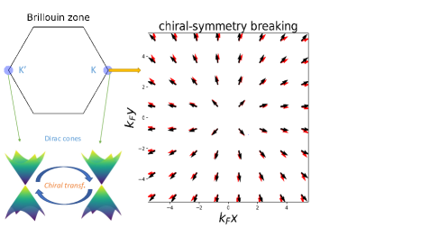
Figure 1: (Color online) The left panel depicts the Brillouin zone of graphene. Around the $K$ and $K^{\prime}$ valleys, the spectrum is Dirac-like, supporting low-energy Hamiltonians $\hat{H}_{K}$ and $\hat{H}_{K^{\prime}}$ that are connected via a chiral transformation, $H_{K}=\hat{\sigma}_{z}H_{K^{\prime}}\hat{\sigma}_{z}$. The right panel depicts the vector field $\mathbf{v}_{K}(\mathbf{r})$ (for definition, see the footnotefoo ), at $K$-valley. The dark (black) vectors field represents the $\mathbf{v}_{K}(\mathbf{r})$ at zero magnetic field. The grey (red) vector field is the $\mathbf{v}_{K}(\mathbf{r})$ at a weak but non-zero magnetic field. Here we take $\omega_{0}/(2E_{F})=0.07$. The figure shows the chiral symmetry of the state at $B=0$. At finite $B$, the chiral-symmetry in one valley is broken. In the leading approximation, the angle between two vector fields is proportional to $\varphi(r)$. Importantly, the chiral transformation leads to the relation, $\mathbf{v}_{K^{\prime}}(\mathbf{r})=\mathbf{v}_{K}(-\mathbf{r})$, manifesting the chiral symmetry of the whole system.

In general, the ballistic correction to the density of states is given by two diagrams shown in Figs. 2a and  2b, which provide comparable contributions. However, as shown in Ref. Mariani et al., 2007, in graphene the Fock diagram dominates over the Hartree diagram in the absence of magnetic field. This is a consequence of the suppressed backscattering. We showapp that the weak magnetic field does not change the picture, namely the Fock diagram is still dominating. We will thus focus on the sensitivity of the Fock diagram to a weak magnetic field.

We start with a matrix generalization of the analytical expressions for the Fock diagram, Fig. 2a. For this purpose, we consider a non-magnetic impurity causing a perturbation $\hat{u}\delta(\mathbf{r})$ and the screened interaction potential, $U(\mathbf{r})$, with a radius $\sim k_{F}^{-1}$. The corresponding expression reads

$$\delta G_{\omega}(\mathbf{r},\mathbf{r})= \int d{\bf r}_{1}d{\bf r}_{2}G_{\omega}(\mathbf{r},\mathbf{r}_{1})H_{\text{F}}(\mathbf{r}_{1},\mathbf{r}_{2})G_{\omega}(\mathbf{r}_{2},\mathbf{0})$$ (4)

$$\times\hat{u}G_{\omega}(\mathbf{0},\mathbf{r})+\left(\hat{u}\leftrightarrow H_{\text{F}}\right).$$

Here $G_{\omega}$ is the free Feynman propagator of the Dirac electrons between the position of impurity ${\bf r}=0$ and the point r), while $H_{F}$ stands for nonlocal Fock potential

$$H_{F}=\frac{i}{2\pi}\int d\Omega G_{\omega+\Omega}(\mathbf{r}_{1},\mathbf{0})\hat{u}G_{\omega+\Omega}(0,\mathbf{r}_{2})U(\mathbf{r_{1}}-\mathbf{r}_{2}).$$ (5)

The interaction correction to the local density of states, $\delta\nu_{\omega}({\bf r})$, is related to the retarded Green’s function as $\delta\nu_{\omega}({\bf r})=-\frac{2}{\pi}\text{Tr~{}Im}~{}\delta G_{\omega}({\bf r},{\bf r}).$

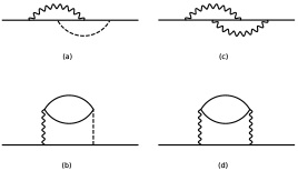
Figure 2: Diagrams for the corrections to the Green function. Solid lines represent the Feynman propagators. Wavy lines represent the electron-electron interactions. (a) represents the Fock diagram involving a single-impurity scattering. It yields a leading contribution to the $B^{2}$ ballistic zero-bias anomaly. (b) represents a Hartree diagram involving a single-impurity scattering. It is insensitive to a weak magnetic field. (c) and (d) represent, respectively, the Fock and Hartree diagrams for the $B^{2}$ correction to the electron lifetime. Unlike the Hartee diagram, which is the first diagram of the RPA sequence, diagram (c) yields an anomalous temperature dependence.

The structure of Eqs. (4), (5) suggests that $\delta\nu_{\omega}({\bf r})$ contains the product of $4\times 4$ matrices. In the semiclassical limit, all trajectories ${\bf r}\rightarrow{\bf r}_{1}\rightarrow{\bf r}_{2}\rightarrow 0\rightarrow{\bf r}$ contributing to $\delta G$ are close to a straight line. With screened Coulomb potential being point-like, the Fock diagram involves the following product of the $M$-matrices

$$F\equiv\text{tr}\left[\hat{u}M(\mathbf{r},+)M(-\mathbf{r},-)\hat{u}M(\mathbf{r},-)M(-\mathbf{r},+)\right].$$ (6)

For a qualitative discussion, let us choose $\hat{u}$ in the form of a scalar, $u_{0}\hat{I}$. Then the leading field-dependent term emerges as a coefficient in front of the product of the projection operators $\text{tr}\left[\hat{\Sigma}_{z}\hat{\Sigma}_{x/y}\hat{\Sigma}_{z}\hat{\Sigma}_{x/y}\right]$. Since the term $\hat{\Sigma}_{z}$ appears in the matrix $M$ in combination with $\varphi(r)$, we have $F\propto\varphi^{2}(r)$. With the help of the commutation relations for ${\hat{\Sigma}_{x}}$, ${\hat{\Sigma}_{y}}$, and ${\hat{\Sigma}_{z}}$, it is easy to check that $\text{tr}\left[\hat{\Sigma}_{z}\hat{\Sigma}_{x/y}\hat{\Sigma}_{z}\hat{\Sigma}_{x/y}\right]=-\text{tr}\left[I\right]$, i.e. it is nonzero. An estimate for $F$ is $\sim u_{0}^{2}\varphi^{2}(r)\sim u_{0}^{2}\omega_{0}^{2}r^{2}/v_{F}^{2}$. With characteristic $r$ being $v_{F}/\omega$, this estimate translates into $u_{0}^{2}\omega_{0}^{2}/\omega^{2}$. Below we examine a number of observables having the structure similar to Eq. (4).

Emerging zero-bias anomaly. For the scalar impurity scattering, $\hat{u}=u_{0}\hat{I}$, there is no zero-bias anomaly in graphene.Mariani et al. (2007) To convert the above estimate for $F$ into the $B$-dependent correction to the density of states, we perform the spatial averaging of Eq. (4), which generates the impurity concentration, $n_{i}$. Final result reads

$$\frac{\delta\nu_{\omega}(B)-\delta\nu_{\omega}(0)}{\nu_{F}}\simeq\frac{\lambda_{0}n_{i}u_{0}^{2}}{8\pi v^{2}_{F}}\frac{\omega_{0}^{2}}{\omega^{2}},$$ (7)

where $\lambda_{0}=k_{F}U_{0}/(2\pi v_{F})$ stands for dimensionless interaction parameter, $U_{0}$ is the interaction potential with zero momentum transfer and $\nu_{F}=k_{F}/(\pi v_{F})$.

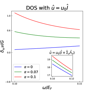
Figure 3: (Color online) Plot (a) and the inset illustrate the energy dependence of the interaction correction to the density of states. Three curves correspond to the three values of the dimensionless magnetic field $\alpha=(k_{F}l)^{-2}$. Plot (a) is for the scalar impurity with magnitude $\hat{u}=u_{0}\hat{I}$. The correction, $\delta\nu$, is measured in the units of $G=\nu_{F}n_{i}(u_{0}/2v_{F})^{2}\lambda_{0}/2\pi$. Note that for $\alpha=0$ the zero-bias anomaly is absent, so that $\delta\nu$ is a smooth function of energy, $\omega$, measured from the Fermi level. In the low-energy regime, $\omega/E_{F}<\sqrt{\alpha}$, the $B$-dependent anomalous term in $\delta\nu$ dominates and behaves as $\sim\alpha^{2}E^{2}_{F}/\omega^{2}$. The inset of Plot (a) is for the impurity-induced perturbation For this perturbation, zero-bias anomaly exists even in the absence of magnetic field. The magnetic contribution yields only a small correction to the logarithmic $\delta\nu$.

The most general form of the point-like perturbation, $\hat{u}$, consistent with time-reversal symmetry is $\hat{u}=u_{0}\hat{I}+\sum_{s,l=x,y,z}u_{sl}\Sigma_{s}\Lambda_{l}$. Here $\Lambda_{x,y}=\hat{\tau}_{x,y}\otimes\hat{\sigma}_{z},\Lambda_{z}=\hat{\tau}_{z}\otimes\hat{\sigma}_{0}$. The remaining nine types of the disorder can be incorporated into Eq. 7 by replacing $u^{2}_{0}$ by $t=u_{0}^{2}-\sum_{l}u^{2}_{zl}$.

The result Eq. 7 was obtained under the assumptions $\omega\tau\gg 1$ and $\omega\gg\omega_{0}$ which ensure the ballistic regime and the irrelevance of the Landau quantization, respectively.

Emergence of a zero-bias anomaly in graphene in the presence of magnetic field manifests itself in the local density of states (DOS), $\delta\nu_{\omega}(\mathbf{r},B)=-2\pi^{-1}\text{ tr}\left[\text{Im }G_{R}(\mathbf{r},\mathbf{r},\omega)\right]$. Evaluation of Eq. (4) yields

$$\frac{\delta\nu_{\omega}(\mathbf{r},B)-\delta\nu_{\omega}(\mathbf{r},0)}{\nu_{F}}\simeq\frac{\lambda_{0}t\omega_{0}^{2}}{(2\pi v_{F}^{2})^{2}}\cos\frac{\omega r}{v_{F}}.$$ (8)

Note that, unlike the $B=0$ case,Mariani et al. (2007) the interaction correction Eq. (8) is isotropic. The most dramatic difference between Eq. (8) and the $B=0$ result is that the zero-field correction falls off as $1/r^{2}$, while the amplitude of oscillations in Eq. (8) does not depend on $r$. Naturally, the fall-off starts from the distances $r\gtrsim R_{L}=v_{F}/\omega_{0}$, where Eq. (8) does not apply. Technically, the extra factor $r^{2}$ comes from $\varphi^{2}(r)$ in the factor $F$. In relation to the local DOS, we would like to point out that it can be measured experimentally using the scanning tunneling microscopy (STM)Marchini et al. (2007); Li et al. (2009).

Quasi-particle lifetime. Energy dependence of electron-electron scattering rate, $\tau_{ee}^{-1}$, in doped graphene is $\omega^{2}\ln\left(E_{F}/\omega\right)$, as in a regular Fermi liquid.Das Sarma et al. (2007) This dependence emerges already in the lowest order of the perturbation theory. Corresponding diagram is illustrated in Fig. 2. Subsequent summation of the higher-order diagrams within the random-phase approximation (RPA) modifies the prefactor in $\tau_{ee}^{-1}$. Equally, the calculations leading to non-analytic interaction correctionsChubukov and Maslov (2003) apply to the doped graphene. With regard to the magnetic field dependence of $\tau_{ee}^{-1}$, it appears that, similarly to the zero-bias anomaly, the leading $B$-dependence originates from the Fock diagram on Fig. 2c, which is beyond the RPA.

The result for the correction, $\delta\tau_{ee}^{-1}(B)$, depends on the ratio $\omega/T$. In the low-$T$ limit, $\omega\gg T$, this correction reads

$$\delta\tau_{ee}^{-1}(B)\simeq\frac{\lambda_{0}\lambda_{2k_{F}}\omega_{0}^{2}}{2\pi E_{F}}\ln\Big{(}\frac{|\omega|}{\Delta}\Big{)},~{}~{}|\omega|\gg T,$$ (9)

where $\lambda_{2k_{F}}=k_{F}U_{2k_{F}}/(2\pi v_{F})$, $\Delta=\text{max}\{T,\tau^{-1}_{ee}\}$. The relative magnitude of the correction is essentially $\left(\omega_{0}/\omega\right)^{2}$ and, similarly to the zero-bias anomaly, it originates from the magnetic phase $\hat{\Sigma}_{z}\varphi(r)$ of the propagator in Feynman diagrams.

In the high-temperature limit, $T\gg\omega$, evaluation of the $B$-dependent correction to the diagram Fig. 2c yields

$$\delta\tau_{ee}^{-1}(B)\simeq-\ln(2)\frac{\lambda_{0}\lambda_{2k_{F}}\omega_{0}^{2}}{2\pi E_{F}},~{}~{}T\gg|\omega|.$$ (10)

Note that the correction is $T$-independent, but it exists on the background of the $T^{2}$ main term.

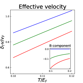
Figure 4: (Color online) In plot the temperature-dependent interaction correction to the effective velocity, $\delta_{T}v^{*}=v_{T}^{*}(B)-v_{T=0}^{*}(B)$ is shown. The inset shows the $B$-dependent component of the effective velocity, $\delta_{T}v^{*}(B)-\delta_{T}v^{*}(0)$. This part behaves as an inverse temperature, $\sim\alpha^{2}E_{F}/T$.

Effective velocity and specific heat. In the doped graphene, as in 2D electron gas, the effective velocity of quasi-particles, $v^{*}$, and specific heat, $C_{v}$, are expected to acquire interaction correctionsChubukov and Maslov (2003); Das Sarma et al. (2007); app . These corrections scale as $\delta v^{*}\propto T$ and $\delta C_{v}\propto T^{2}$, respectively. Both anomalies originate from the non-analytic corrections to the quasi-particle lifetime Chubukov and Maslov (2003). Here we trace how the $\omega_{0}^{2}$-corrections specific for graphene manifest themselves in $v^{*}$ and $C_{v}$. The question of interest is the temperature dependence of these corrections. We found that the correction to $v^{*}$ behaves as $\omega_{0}^{2}/T$, while the correction to $C_{v}$ is $\propto\omega_{0}^{2}/v_{F}^{2}$ and is $T$-independent. Both originate from $\omega_{0}^{2}$ correction to the lifetime given by Eqs. 9 and  10.

Another ingredient required to find the $B$-dependent corrections to $v^{*}$ and $C_{v}$ is the electron spectrum renormalized by the interactions. The corresponding $\omega_{0}^{2}$-correction comes from the Fock diagram Fig. 2c

$$\text{Re}[\Sigma(\omega,B)-\Sigma(\omega,0)]\simeq-\frac{\lambda_{0}\lambda_{2k_{F}}\omega_{0}^{2}}{16E_{F}}\times\left\{\begin{array}[]{cc}\text{sgn}(\omega),&\text{$|\omega|\gg T$}\\ \omega/(2T),&\text{$|\omega|\ll T$}.\\ \end{array}\right.$$ (13)

The above correction can, in principle, be measured using the Angle-resolved photoemission spectroscopy (ARPES)Lv et al. (2019) from the analysis of the constant energy mapsMucha-Kruczyński et al. (2008) at different values of $B$.

In the limit $T\gg\omega$, the renormalized spectrum Eq. 13 leads to the following correction to the effective velocity of quasi-particles $v=v_{F}/\left(1-\partial_{\omega}\text{Re}\Sigma|_{\omega=0}\right)$,app

$$\frac{v(B)-v(0)}{v_{F}}\simeq-\frac{\lambda_{0}\lambda_{2k_{F}}\omega_{0}^{2}}{32E^{2}_{F}}\frac{E_{F}}{T}.$$ (15)

Note that $v(0)$ contains a non-magnetic interaction correction which is linear in $T$. On the contrary, the $B$-dependent correction is $\propto T^{-1}$. This feature is illustrated in Fig. 4 for several values of $B$. Since the thermodynamical potential, $\Omega$, involves the summation over energies of quasi-particles near the Fermi level, the energy correction in Eq. 13 has non-trivial implications for thermodynamics. Here we consider the specific heat per unit volume, $C_{v}=V^{-1}\partial\Omega/\partial T$, where $V$ is the volume of system. The result for specific heatapp in the limit $T\gg\omega_{0}$ is the following,

$$\delta C_{v}(B)-\delta C_{v}(0)\simeq-\frac{\lambda_{0}\lambda_{2k_{F}}\omega_{0}^{2}}{8\pi v_{F}^{2}},$$ (16)

where $\delta C_{v}(B)$ is the interaction correction to the specific heat. Note that $\delta C_{v}(0)$ contains the conventional $T^{2}$ term, specific for 2D Fermi liquid. We find that the field-dependent correction to $\delta C_{v}$ is a $T$-independent. In the absence of electron-phonon interactions, the field-dependent correction exists in a parametrically large interval of temperatures, $\omega_{0}<T<E_{F}$. Eq. 16 can be verified experimentally by measuring the specific heat of graphene in a comprehensive Raman optothermal methodLi et al. (2017).

Conclusion. Our main finding is that, for two-dimensional Dirac electrons, application of a weak magnetic field enhances significantly the many-body effects. This is unlike the conventional 2D electron gas. The reason for this is the pseudospin-dependent magnetic correction in Dirac electron propagators, $\sim\hat{\Sigma}_{z}\varphi(r)$. For many-body effects to unfold, the energy, $\omega$, measured from the Fermi level should exceed $\omega_{0}=v_{F}(k_{F}l^{2})^{-1}$, which is the inter-Landau-level distance at the Fermi level. We have only considered the low-temperature properties of interacting electrons in the doped graphene, so that the interaction with phononsSedrakyan et al. (2021); Faugeras et al. (2010) can be neglected.

Our predictions for observables given by Eqs. 9-16 and by Eq. 7 all emerge as a result of evaluation of the Fock diagrams illustrated in Figs. 2a, 2c. It is nontrivial that, while these diagrams are not leading and even do not belong to the RPA sequence, they are responsible for the sensitivity to a weak magnetic field. Importantly, the higher-order diagrams,while leading to the renormalization of the interaction vertex, do not modify thepredicted $\omega,T$-dependencies.

Other origin of the $B$-dependence of the interaction effects is either spin via the Zeeman splitting coming from spin or or the orbital effect via the curving of the electron trajectories in magnetic field. We have checkedapp that these two mechanisms lead to the $B$-dependent corrections which are sub-leading compared to the ones originating from the pseudospin-dependent phase of Dirac propagators.

Finally, we emphasize that our results apply for the doped graphene, where the Fermi energy is far away from the neutrality. The condition $\omega\gg\omega_{0}$ in the present letter is automatically violated at neutrality. The question about $\nu=0$ Landau level is interesting and remains openKharitonov (2012); Goerbig (2011).

Acknowledgements. The research was supported by startup funds from the University of Massachusetts, Amherst (K.W. and T.A.S.), and by the Department of Energy, Office of Basic Energy Sciences, Grant No. DE-FG02-06ER46313 (M.E.R.).

Supplemental Material: Interaction effects in Graphene in a weak magnetic field

I Dirac propagator in the presence of a weak magnetic field

This section provides a derivation of the Dirac propagator for the $K$-valley using the operator formalism. In the presence of magnetic field, the spectrum of the Dirac electrons transforms into the ladders of Landau levels. The level positions are given by $\omega_{n}=\sqrt{2n}v_{F}/l$, where $v_{F}$ is the Fermi velocity and $l$ is the magnetic length. The corresponding wavefunctions in the $K$-valley are given by $\psi_{n,k_{x}}(\mathbf{z})=\frac{1}{\sqrt{2}}\Big{(}\varphi_{n-1,k_{x}}(\mathbf{z}),-\varphi_{n,k_{x}}(\mathbf{z})\Big{)}$, where $\varphi_{n,k_{x}}(\mathbf{z})$ is the wavefunction of $n^{\text{th}}$ Landau level of the 2D electrons.

To calculate the propagator, it is sufficient to consider the group of levels around $E_{F}$. Then the definition of the propagator leads to the following starting expression:

$$G_{K}^{s,s^{\prime}}(\mathbf{z},\mathbf{z^{\prime}};\omega)\simeq\int\frac{dk_{x}}{2\pi}\sum_{n}\psi^{s}_{n,k_{x}}(\mathbf{z})\psi^{s^{\prime},*}_{n,k_{x}}(\mathbf{z^{\prime}})\times\frac{1}{\omega-\omega_{n}+i\delta\Theta(\omega-E_{F})}.$$ (S1)

Here $\mathbf{z}=(x,y)$, $\mathbf{z}^{\prime}=(x^{\prime},y^{\prime})$, while the indices $s$ and $s^{\prime}$ taking the values $s,s^{\prime}=\pm$ refer to the $A/B$ sublattices.

The off-diagonal propagators could be expressed in terms of diagonal ones via the following expression $G^{s,s^{\prime}}_{K}(\mathbf{z},\mathbf{z^{\prime}},\omega)=\frac{l^{2}\omega{p}_{s^{\prime}}}{v_{F}r^{2}}\left[G^{11}_{K}(\mathbf{z},\mathbf{z^{\prime}},\omega)-G^{22}_{K}(\mathbf{z},\mathbf{z^{\prime}},\omega)\right]$ with $\tilde{p}_{\pm}={\pm(y-y^{\prime})-i(x-x^{\prime})}$. Thus, we focus on the summation over the Landau levels for diagonal propagators. Upon substituting the expression of $\psi_{n,k_{x}}(\mathbf{x})$ and variable change $n\rightarrow n-(s+1)/2$, we obtain

$$G_{K}^{s,s}(\mathbf{x},\mathbf{x^{\prime}};\omega)\simeq\frac{1}{2}\int\frac{dk_{x}}{2\pi}\sum_{n}\varphi_{n,k_{x}}(\mathbf{x})\varphi^{*}_{n,k_{x}}(\mathbf{x^{\prime}})\frac{1}{\omega-\omega_{n+(s+1)/2}}.$$ (S2)

Next we expand $\omega_{n+(s+1)/2}=\sqrt{2n+(s+1)}v_{F}/l$ around the Fermi energy and find

$$\omega_{n+(s+1)/2}\simeq E_{F}\Big{(}1+\frac{s}{2k_{F}^{2}l^{2}}\Big{)}+(\delta n+1/2)\frac{E_{F}}{k_{F}^{2}l^{2}}.$$

Here we introduce an effective Fermi energy $E_{F}(1+s(2k_{F}^{2}l^{2})^{-1})$ and effective cyclotron frequency $\omega_{0}=E_{F}/k_{F}^{2}l^{2}$. Subsequently, the effective Fermi energy introduces an effective momentum as $k_{F}^{s,s}=E^{s}_{F}/v_{F}$. One readily finds: $k_{s,s}=k_{F}^{s,s}(1+s(2k_{F}^{2}l^{2})^{-1})$.

The effective momentum in the off-diagonal Green functions is exactly the Fermi momentum. Thus, we can keep the off-diagonal propagators the same as the ones without magnetic field. The diagonal Dirac propagators can be identified with the 2D electron gas propagator with the effective momentum $k_{F}^{s,s}$. Upon the use of the expression of the propagator of the 2D electron gasSedrakyan et al. (2007), one finds

$$G(\mathbf{z},\mathbf{z}^{\prime};\omega)\simeq e^{-i\chi}I(\mathbf{z}-\mathbf{z}^{\prime};\omega)\hat{M}(\mathbf{z}-\mathbf{z}^{\prime};\text{sgn}(\omega)),$$ (S3)

where $I(\mathbf{z}-\mathbf{z}^{\prime};\omega)=\frac{1}{2v_{F}}\sqrt{\frac{k_{F}}{2\pi r}}\exp i\text{sgn}(\omega)\left(k_{F}r+\frac{\omega}{v_{F}}r+\frac{\pi}{4}-\frac{r^{3}}{24k_{F}l^{4}}\right).$ Here $r=|\mathbf{z}-\mathbf{z^{\prime}}|$, $\chi=(x-x^{\prime})(y+y^{\prime})/(2l^{2})$ describe the breaking of the translational invariance. The matrix reads as

$${M}\left(\mathbf{r};\text{sgn}(\omega)\right) \simeq \Big{(}\text{sgn}(\omega)+\frac{i}{2k_{F}r}\Big{)}\hat{r}\cdot\boldsymbol{\Sigma}+\exp\Big{\{}-i\text{sgn}(\omega)\varphi(r)\hat{\Sigma}_{z}\Big{\}},$$ (S4)

where $\hat{r}=\mathbf{r}/r$, $\Sigma_{x,y}=\sigma_{x,y}\otimes\tau_{z}$, $\varphi(r)=r/(2k_{F}l^{2})$ and $\Sigma_{z}=\sigma_{z}\otimes\tau_{0}$. Here $\sigma$ acts on the pseudo-spin space and $\tau$ acts on the valleys. Expanding the exponents up to $\varphi^{2}$, one recovers the expression of Eq. (2) from the main text. The result in Eq. S4 applies when $k^{-1}_{F}<r<k_{F}l^{2}$.

II Hartree v.s. Fock diagrams

In the main-text, we argue that Fock diagram (which is a non-RPA diagram) gives leading field-dependent corrections while Hartree diagram contribution is subleading. This property comes from the fact that the back-scattering, which is the relevant process for the Hartree diagram, is suppressed in the graphene. Here we provide a detailed calculation when one consider quasi-particle lifetime. For other physical quantities (e.g. )

• When one use Hartree diagram to evaluate the quasi-particle life- time, one needs to consider the product of two dynamical polarization operator. The species with $2k_{F}$ momentum transfer in the Hartree diagram contains the following product of matrices

  $$H\equiv\text{tr}\left[M(\mathbf{r},+)M(-\mathbf{r},+)\right]\times\text{tr}\left[M(\mathbf{r},-)M(-\mathbf{r},-)\right].$$ (S5)

  Using $M$ in Eq. S4, one could recover the following equation

  $$\text{tr}\left[M(\mathbf{r},s)M(-\mathbf{r},s)\right]=4\Big{(}-1-i\frac{s}{k_{F}r}+\cos\varphi(r)\Big{)}\simeq-4\Big{(}i\frac{s}{k_{F}r}+\frac{\varphi(r)^{2}}{2}\Big{)}$$ (S6)

  Note that the cancellation of leading term in $-1+\cos\varphi$ is the result of the suppression of the back-scattering (and then the faster decaying term $1/(k_{F}r)$ plays a important role in graphene). One may put Eq. S6 into Eq. S5 and obtain

  $$H\simeq 16\Big{(}\frac{i}{k_{F}r}+\frac{\varphi(r)^{2}}{2}\Big{)}\Big{(}-\frac{i}{k_{F}r}+\frac{\varphi(r)^{2}}{2}\Big{)}$$ (S7)

  One can clearly observe that the crossing term, which is proportional to $\varphi^{2}(\propto B^{2})$, vanishes. Even if the crossing term does not vanish, the extra decaying power $r^{-1}$ in Eq. S6 makes the cross term in Hartree’s contribution sub-leading compared to Fock’s one, which will be calculated below.

• In the Fock diagram, the forward scattering becomes the relevant process. The following product of matrices is involved

  $$F\equiv\text{tr}\left[M(\mathbf{r},+)M(-\mathbf{r},-)M(\mathbf{r},-)M(-\mathbf{r},+)\right].$$ (S8)

  Using $M$ in Eq. S4, one could recover the following equation

  $$M(\mathbf{r},+)M(-\mathbf{r},-)=2\Big{(}1+\hat{r}\cdot\boldsymbol{\Sigma}\exp\{i\varphi(r)\Sigma_{z}\}\Big{)}$$ (S9)

  Then put the equation above into $F$ and one obtains

  $$F=16\Big{(}1-\cos\varphi(r)\Big{)}\simeq 8\varphi(r)^{2}$$ (S10)

  Thus one could observe that $F$ in Eq. S10 give stronger contribution than $H$ in Eq. S7.

III Derivation of the DOS

We start from the standard expression for the density of states, $\nu(\omega;B)$, in terms of the retarded Green function

$$\nu(\omega;B)=-\frac{2}{\pi}\int d^{2}r\textbf{Im}\textbf{tr}G_{R}(\mathbf{r},\mathbf{r};\omega).$$ (S11)

In the ballistic regime, the interaction correction to $\nu(\omega;B)$ is given by the Fock and the Hartree diagrams depicted in Figs. 2a and 2c, respectively. Specifics of graphene is the absence of the backscattering. As a result, the Hartree diagram, which is dominated by the backscattering, does not lead to the zero-bias anomaly. Analytical expression for the Fock diagram reads

$$\delta_{f}G(\mathbf{r},\mathbf{r};\omega)\simeq i2U\int d^{2}r_{1}\int_{-E_{F}}^{-\omega}\frac{d\Omega_{1}}{2\pi}G(\mathbf{r},\mathbf{r}_{1};\omega)G(\mathbf{r}_{1},0;\omega+\Omega_{1})$$

$$\times\hat{u}G(0,\mathbf{r}_{1};\omega+\Omega_{1})G(\mathbf{r}_{1},0;\omega)\hat{u}G(0,\mathbf{r};\omega).$$ (S12)

Here we consider the touching potential. Thus the interaction potential in momentum space is uniform, namely, a single number $U$. In Eq. (III) we assume that $\omega$ is positive and use the Green function, $G$, instead of $G_{R}$.

Spatial averaging of $\delta_{f}G(r,r)$ is accomplished with the help of the following identity

$$\int d^{2}rG(0,\mathbf{r};\omega)G(\mathbf{r},\mathbf{r}_{1};\omega)=-\partial_{\omega}G(0,\mathbf{r}_{1};\omega).$$ (S13)

Another simplification comes from the fact that the distances contributing to the integral Eq. (III) are large, so that the Green function can be replaced by the semiclassical asymptote

$$\partial_{\omega}G(0,\mathbf{r}_{1};\omega)\simeq i\text{sgn}(\omega)\frac{r_{1}}{v_{F}}G(0,\mathbf{r}_{1};\omega).$$ (S14)

Subsequent steps are in line with the calculation in Phys. Rev. B 76, 165402 (2007). They involve substituting the asymptotic expressions for the Green functions into $\delta_{f}\nu(\omega;B)$, calculating the product of matrices entering the Green functions and integrating out the intermediate frequency $\Omega_{1}$. As a result, the expression for $\delta_{f}\nu(\omega;B)$ simplifies to

$$\delta_{f}\nu(\omega;B) = -2n_{i}U_{0}\textbf{Re}\int d\theta dr_{1}\frac{k^{2}_{F}}{32\pi^{4}v^{4}_{F}}\frac{1}{r_{1}}e^{2i\omega r_{1}/v_{F}}\times\textbf{tr}(\hat{u}^{2}-\hat{\Sigma}(\psi)\hat{u}\hat{\Sigma}(\bar{\psi})\hat{u}),$$ (S15)

where $n_{i}$ is the impurity concentration. In Eq. (S15) the angle $\theta$ is the angular coordinate of $\mathbf{r}_{1}$, while the angles $\psi,\bar{\psi}$ are defined as

$$\psi=\theta+\varphi(r_{1}),\quad\bar{\psi}=\theta-\varphi(r_{1}).$$ (S16)

Finally, the function $\hat{\Sigma}$ is expressed via $\psi$, $\bar{\psi}$ as follows

$$\hat{\Sigma}(\psi)=(\cos\psi,\sin\psi)\cdot(\hat{\Sigma}_{x},\hat{\Sigma}_{y}).$$ (S17)

Eq. (S15) illustrates how the magnetic phase, $\varphi(r_{1})$, from the electron propagator enters the interaction correction to the density of states.

To explore the magnetic field dependence, we analyze the intermediate integral

$$\int\frac{d\theta}{2\pi}\textbf{tr}(\hat{u}^{2}-\Sigma(\psi)\hat{u}\Sigma(\bar{\psi})\hat{u})\simeq 4\sum_{l=x,y,z}(2u^{2}_{zl}+u^{2}_{yl}+u^{2}_{xl})+t\frac{2r_{1}^{2}}{k_{F}^{4}l^{4}}.$$ (S18)

Here $t=u^{2}-\sum_{l}u^{2}_{zl}$. From the above expression, one concludes that only the scalar potentials, including $u,u_{zz},u_{zx}$ and $u_{zy}$, are sensitive to the magnetic field. Defining a dimensionless variable $x=2\omega r_{1}/v_{F}$, we cast the magnetic-field correction in the form of a single integral over $x$

$$\frac{\delta_{f}\nu(\omega;B)-\delta_{f}\nu(\omega;0)}{\nu_{F}}=-\frac{k_{F}U_{0}}{v_{F}}\frac{t}{16\pi^{2}v^{2}_{F}v}\frac{\omega_{0}^{2}}{\omega^{2}}\int_{2\omega/E_{F}}^{2\omega/\omega_{0}}xe^{-\epsilon x}\cos xdx.$$ (S19)

Here $\epsilon$ is introduced as a cutoff. In the limit $\omega_{0}\ll\omega\ll E_{F}$, we get

$$\frac{\delta_{f}\nu(\omega;B)-\delta_{f}\nu(\omega;0)}{\nu_{F}}\simeq n_{i}\frac{k_{F}U_{0}}{v_{F}}\frac{t}{16\pi^{2}v^{2}_{F}}\frac{\omega_{0}^{2}}{\omega^{2}}.$$ (S20)

We thus arrive to Eq. (8) of the main text.

IV Self-energy calculation at finite temperature

In this section, we provide a detailed calculation of the self-energy at finite temperature. The diagrams we consider are shown in Fig. 2 of the main text. The calculation presented here is performed for a single spin. At finite temperature, the asymptotic expression for the propagator reads

$$G(\mathbf{z},\mathbf{z}^{\prime};i\omega_{n})\simeq e^{-i\chi}I(\mathbf{z}-\mathbf{z}^{\prime};i\omega_{n})\hat{M}(\mathbf{z}-\mathbf{z}^{\prime};\text{sgn}(n)),$$ (S21)

where $i\omega_{n}$ is the fermionic Matsubara frequency. The function $\chi$ is defined by Eq. (S3).

IV.1 Hartree and Fock diagrams

In the coordinate space, the Hartree and Fock corrections to the self-energy are, respectively, given by the summation over bosonic Matsubara frequencies

$$\Sigma_{\text{Hartree}}(\mathbf{x}_{1},\mathbf{x}_{2};i\omega_{n}) \simeq -TU^{2}\sum_{i\nu_{m}}G(\mathbf{x}_{1},\mathbf{x}_{2},i\omega_{n}-i\nu_{m})\Pi(\mathbf{x}_{2}-\mathbf{x}_{1},i\nu_{m}),$$ (S22)

$$\Sigma_{\text{Fock}}(\mathbf{x}_{1},\mathbf{x}_{2};i\omega_{n}) \simeq T^{2}U^{2}\sum_{i\nu_{m},i\nu_{l}}G(\mathbf{x}_{1},\mathbf{x}_{2};i\omega_{n}-i\nu_{m})G(\mathbf{x}_{2},\mathbf{x}_{1};i\omega_{n}-i\nu_{m}-i\nu_{l})G(\mathbf{x}_{1},\mathbf{x}_{2};,i\omega_{n}-i\nu_{l}).$$

Here $U$ is the short-ranged interaction potential (touching potential) in momentum space, $\nu_{m}=2\pi Tm$ and $\Pi(\mathbf{x}_{2}-\mathbf{x}_{1},i\nu_{m})$ is the polarization operator. Since the chiral structure of graphene suppresses the backscattering process, we focus on the zero-momentum species of polarization operator $\Pi_{0}$,

$$\Pi_{0}(\mathbf{x_{2}},\mathbf{x_{1}};i\nu_{m}) = \frac{k_{F}^{2}}{2\pi^{2}v_{F}^{2}}\frac{1}{k_{F}r}|\nu_{m}|e^{-|\nu_{m}|r/v_{F}}.$$ (S23)

Here we introduced $r=|\mathbf{x_{2}}-\mathbf{x_{1}}|$. Further, we consider quasi-particles characterized by index $\nu$ ($\nu$ is characterized by the momentum for a free particle in the absence of the $B$-field and the Landau level index in the presence of the magnetic field). Then the self-energy is defined by

$$\Sigma(\nu,i\omega_{n})=\textbf{tr}\int d^{2}x_{1}d^{2}x_{2}A(\mathbf{x}_{2},\mathbf{x}_{1},\nu)\Sigma(\mathbf{x}_{1},\mathbf{x}_{2},i\omega_{n})/\Big{(}Vk_{F}/2\pi v_{F}\Big{)},$$ (S24)

where $A$ is the spectral function of electrons in the absence of interaction and $V$ is the volume of the system. The spectral function is defined from by $A=-(2\pi i)^{-1}(G_{R}-G_{A})$. Here $G_{R/A}$ are the retarded/advanced non-interacting Green functions. Taking an analytic continuation $i\omega_{n}\rightarrow\omega+i\delta$ (consider the case with $\omega>0$) and separating the on-shell singularity, we obtain

$$\Sigma_{\text{Hartree}}(\omega+i\delta)\simeq i\Big{(}\frac{k_{F}U}{v_{F}}\Big{)}^{2}\frac{T}{2\pi^{2}E_{F}}\int\frac{e^{-\delta r/v_{F}}dr}{r}\Bigg{[}\frac{\pi T}{\sinh^{2}(2\pi Tr/v_{F})}-$$

$$\frac{e^{i2\omega r/v_{F}}}{\sinh(2\pi Tr/v_{F})}\Big{(}-i\omega+\frac{\pi T}{\tanh(2\pi Tr/v_{F})}\Big{)}\Bigg{]},$$

and

$$\Sigma_{\text{Fock}}(\omega+i\delta) \simeq -i\Big{(}\frac{k_{F}U}{v_{F}}\Big{)}^{2}\frac{T}{2\pi^{2}E_{F}}\int dr\frac{e^{-\delta r/v_{F}}\sin^{2}\varphi(r)}{r}\Bigg{[}\frac{\pi T}{\sinh^{2}(2\pi Tr/v_{F})}-$$ (S25)

$$\frac{e^{i2\omega r/v_{F}}}{\sinh(2\pi Tr/v_{F})}\Big{(}-i\omega+\frac{\pi T}{\tanh(2\pi Tr/v_{F})}\Big{)}\Bigg{]}.$$

IV.2 $T/\omega\ll 1$

For small $T/\omega\ll 1$, the $\Sigma_{\text{Hartree}}$ is simplified to

$$\Sigma_{\text{Hartree}}(\omega+i\delta)\simeq i\Big{(}\frac{k_{F}U}{v_{F}}\Big{)}^{2}\frac{1}{4\pi^{3}}\int dr\frac{e^{-\delta r/v_{F}}dr}{k_{F}r^{2}}\Bigg{[}\frac{v_{F}}{2r}-e^{i2\omega r/v_{F}}\Big{(}-i\omega+\frac{v_{F}}{2r}\Big{)}\Bigg{]},$$ (S26)

and the $\Sigma_{\text{Fock}}$ becomes

$$\Sigma_{\text{Fock}}(\omega+i\delta)\simeq-i\Big{(}\frac{k_{F}U}{v_{F}}\Big{)}^{2}\frac{1}{4\pi^{3}}\int dr\frac{e^{-\delta r/v_{F}}dr}{k_{F}r^{2}}\Bigg{[}\frac{v_{F}}{2r}-e^{i2\omega r/v_{F}}\Big{(}-i\omega+\frac{v_{F}}{2r}\Big{)}\Bigg{]}\sin^{2}\varphi(r).$$

• Quasiparticle lifetime. Here we calculate the imaginary part of the self-energy and find the expression for the lifetime. Defining dimensionless quantity $x=2\omega r/v_{F}$, we write $\Sigma_{\text{Hartree}}(\omega+i\delta)$ as

  $$\textbf{Im}\Sigma_{\text{Hartree}}(\omega+i\delta)\simeq\Big{(}\frac{k_{F}U}{v_{F}}\Big{)}^{2}\frac{\omega^{2}}{2\pi^{3}E_{F}}\int^{+\infty}_{2\omega/E_{F}}dx\Big{(}\frac{1}{x^{3}}[1-\cos x]-\frac{1}{x^{2}}\sin x\Big{)}.$$ (S27)

  The leading term in the integral $\int^{+\infty}_{2\omega/E_{F}}dx\Big{(}\frac{1}{x^{3}}[1-\cos x]-\frac{1}{x^{2}}\sin x\Big{)}$ is $2^{-1}\log(2\omega/E_{F})$. Thus one obtains $\textbf{Im}\Sigma_{\text{Hartree}}(\omega+i\delta)\simeq\Big{(}\frac{k_{F}U}{v_{F}}\Big{)}^{2}\frac{\omega^{2}}{4\pi^{3}E_{F}}\log(2\omega/E_{F})$, which is the typical behavior of the lifetime of 2D Fermi liquids. The scattering rate $\delta=-\tau^{-1}_{\text{ee}}/2$ is estimated by the RPA diagrams which give the leading contribution to the lifetime of quasi-particles. Now we study the $B$-dependence of the lifetime. We consider the weak magnetic field such that the mean free path is smaller than the Lamour radius ($\delta>\omega_{0}$). Consider two cases.

  The first case is $T\ll\tau^{-1}_{\text{ee}}$. In this limit, the temperature is an irrelevant scale and the RPA lifetime dominates. We obtain the following equation fo the field-dependent self-energy term:

  $$\textbf{Im}\Sigma_{\text{Fock}}(\omega+i\delta)\simeq-\Big{(}\frac{k_{F}U}{v_{F}}\Big{)}^{2}\frac{\omega_{0}^{2}}{16\pi^{3}E_{F}}\int^{+\infty}_{2\omega/E_{F}}\frac{e^{-\epsilon x}dx}{x}\Big{[}1-\cos x\Big{]}.$$ (S28)

  Here $\epsilon=\delta/2\omega$. The leading term in the integral $\int^{+\infty}_{2\omega/E_{F}}\frac{e^{-\epsilon x}dx}{x}\Big{[}1-\cos x\Big{]}$ giving $\log(2\omega\tau_{\text{ee}})$.

  The second case is $T\gg\tau^{-1}_{\text{ee}}$. In this limit, the temperature enters under the logarithm replacing the inverse lifetime there. Using the relation $\tau^{-1}=-2\textbf{Im}\Sigma$, the similar calculation yields the expression for lifetime given by Eq. 9 of the main-text.

• Spectrum. The real part of the self-energy gives a correction to the spectrum of quasi-particles. Thus here we compute $\textbf{Re}\Sigma_{\text{Hartree}}$ and $\textbf{Re}\Sigma_{\text{Fock}}$

  $$\textbf{Re}\Sigma_{\text{Hartree}}(\omega+i\delta)\simeq\Big{(}\frac{k_{F}U}{v_{F}}\Big{)}^{2}\frac{1}{2\pi^{3}}\frac{\omega^{2}}{E_{F}}\int_{2\omega/E_{F}}^{+\infty}dx\Big{[}-\frac{1}{x^{2}}\cos x+\frac{1}{x^{3}}\sin x\Big{]}.$$ (S29)

  The leading term in integral $\int_{2\omega/E_{F}}^{+\infty}dx\Big{[}-\frac{1}{x^{2}}\cos x+\frac{1}{x^{3}}\sin x\Big{]}$ is simply a constant, given by $\pi/4$. Thus this leads to $\textbf{Re}\Sigma_{\text{Hartree}}(\omega+i\delta)\simeq\Big{(}\frac{k_{F}U_{0}}{v_{F}}\Big{)}^{2}\frac{1}{8\pi^{2}}\frac{\omega^{2}}{E_{F}}$ and

  $$\textbf{Re}\Sigma_{\text{Fock}}(\omega+i\delta)\simeq\Big{(}\frac{k_{F}U}{v_{F}}\Big{)}^{2}\frac{1}{32\pi^{3}}\frac{\omega^{2}_{0}}{E_{F}}\int_{2\omega/E_{F}}^{\omega/\omega_{0}}dxe^{-\epsilon x}\Big{(}\cos x-\frac{1}{x}\sin x\Big{)}.$$

  Then we extend the integral from $0$ to $\infty$, since $\omega/E_{F}\ll 1$ and $\epsilon\omega/\omega_{0}\gg 1$. This yields

  $$\textbf{Re}\Sigma_{\text{Fock}}(\omega)\simeq-\Big{(}\frac{k_{F}U}{v_{F}}\Big{)}^{2}\frac{1}{(8\pi)^{2}}\frac{\omega^{2}_{0}}{E_{F}}.$$ (S30)

  The expression is valid when $\tau_{\text{ee}}^{-1}(\omega)>\omega_{0}$. This introduces the correction to the quasi-particle spectrum in the low temperature limit, shown in Eq. 11. If one considers $\omega<0$, one will restore a $\text{sgn}(\omega)$ to Eq. S15.

IV.3 $T/\omega\gg 1$

In case of large $T/\omega\gg 1$, the temperature is a relevant scale.

• Lifetime. Here we compute the imaginary part of the self-energy to find the quasiparticle lifetime. Defining dimensionless variable $x=\pi Tr/v_{F}$, we write $\Sigma_{\text{Hartree}}(\omega)$ as

  $$\textbf{Im}\Sigma_{\text{Hartree}}\simeq-\Big{(}\frac{k_{F}U}{v_{F}}\Big{)}^{2}\frac{T^{2}}{4\pi E_{F}}\int^{+\infty}_{\pi T/E_{F}}\frac{dx}{x}\frac{1}{\cosh^{2}x}.$$ (S31)

  The integral $\int^{+\infty}_{\pi T/E_{F}}\frac{dx}{x}\frac{1}{\cosh^{2}x}$ is equal to $\log(E_{F}/\pi T)+c+O(T/E_{F})$. Here $c$ is a constant. Thus we find $\textbf{Im}\Sigma_{\text{Hartree}}\simeq\Big{(}\frac{k_{F}U_{0}}{v_{F}}\Big{)}^{2}\frac{T^{2}}{4\pi E_{F}}\log(\pi T/E_{F})$, a typical result for 2D Fermi-liquids. Meanwhile, one could write $\Sigma_{\text{Fock}}(\omega)$ as

  $$\textbf{Im}\Sigma_{\text{Fock}} \simeq \Big{(}\frac{k_{F}U}{v_{F}}\Big{)}^{2}\frac{1}{4\pi^{3}}\frac{\omega^{2}_{0}}{4E_{F}}\int_{\pi T/E_{F}}^{\infty}dx\frac{x}{\cosh^{2}x}.$$

  The integral $\int_{\pi T/E_{F}}^{\infty}dx\frac{x}{\cosh^{2}x}=\log(2)+O(T^{2}/E_{F}^{2})$. Thus $\textbf{Im}\Sigma_{\text{Fock}}\simeq\Big{(}\frac{k_{F}U_{0}}{v_{F}}\Big{)}^{2}\frac{1}{4\pi^{3}}\frac{\omega^{2}_{0}}{4E_{F}}\log(2)$. This gives the correction to the lifetime, written in Eq. 10 of the main-text.

• Spectrum. The real part of $\Sigma_{\text{Hartree}}$ is given by

  $$\textbf{Re}\Sigma_{\text{Hartree}}(\omega+i\delta)\simeq-\Big{(}\frac{k_{F}U}{v_{F}}\Big{)}^{2}\frac{\omega T}{2\pi^{2}E_{F}}\int_{2\pi T/E_{F}}^{\infty}\frac{dx}{x}\frac{1}{\sinh x}\Big{(}1-\frac{x}{\tanh x}\Big{)}.$$

  The integral $\int_{2\pi T/E_{F}}^{\infty}\frac{dx}{x}\Big{[}\frac{1}{\sinh x}\Big{(}1-\frac{x}{\tanh x}\Big{)}\Big{]}=-\log(2)+O(T/E_{F})$. Thus we find that $\textbf{Re}\Sigma_{\text{Hartree}}(\omega+i\delta)\simeq\Big{(}\frac{k_{F}U_{0}}{v_{F}}\Big{)}^{2}\frac{\omega T}{2\pi^{2}E_{F}}\log(2)$. This is also a typical result for 2D Fermi liquids. Then we consider the Fock diagram and write $\textbf{Re}\Sigma_{\text{Fock}}$ as

  $$\textbf{Re}\Sigma_{\text{Fock}}(\omega+i\delta) \simeq \Big{(}\frac{k_{F}U}{v_{F}}\Big{)}^{2}\frac{\omega\omega_{0}^{2}}{32\pi^{4}E_{F}T}\int_{2\pi T/E_{F}}^{2\pi T/\omega_{0}}dx\times x\frac{1}{\sinh x}\Big{(}1-\frac{x}{\tanh x}\Big{)}.$$ (S32)

  Since $T/E_{F}\ll 1$ and $T/\omega\gg 1$, we can replace the lower bound of the integral domain by $0$ and the upper bound by $\infty$. Making use of the integral $\int_{0}^{+\infty}dxx\frac{1}{\sinh x}\Big{(}1-\frac{x}{\tanh x}\Big{)}=-\pi^{2}/4$, we obtain at $T\gg\omega,\omega_{0}$:

  $$\textbf{Re}\Sigma_{\text{Fock}}(\omega+i\delta) \simeq -\Big{(}\frac{k_{F}U}{v_{F}}\Big{)}^{2}\frac{\omega}{2(8\pi)^{2}}\frac{\omega_{0}^{2}}{E^{2}_{F}}\times\frac{E_{F}}{T}.$$ (S33)

  Equations  S30 and  S33 result in Eq. (11) of the main text.

  The velocity of quasi-particle might be obtained by Fourier transforming Eq. S3 by $(2\pi)^{-1}\int d\omega G(\omega)\exp(i\omega t)$. One obtains a delta-funtion $\delta(r-v_{F}t)$ after the transformation. This indicates that the velocity of quasi-particle is $v_{F}$ in the semi-classical regime, even in the presence magnetic field. In the presence of interaction, the spectrum of quasi-particle is corrected. Thus the propagator in Eq. S3 obtains interaction correction. Now the exponential part in $G(\omega)$ becomes $\exp i\Big{(}\omega-\textbf{Re}\Sigma(\omega)\Big{)}r/v_{F}$, where $\Sigma$ is the self-energy correction, containing both Hartree and Fock corrections. Then the Fourier transformation leads a delta function, $\delta\left(\left(1-\partial_{\omega}\textbf{Re}\Sigma|_{\omega=0}\right)r-v_{F}t\right)$. Thus the velocity got renormalzied by the interaction to be $v_{F}/\left(1-\partial_{\omega}\textbf{Re}\Sigma|_{\omega=0}\right)\simeq v_{F}(1+\partial_{\omega}\textbf{Re}\Sigma|_{\omega=0})$. Since the field-dependence correction comes from Eq. S33, one then uses Eq. S33 to obtain the field-dependent correction to effective velocity and then recovers Eq. 12 in the main text.

V Derivation of the specific heat

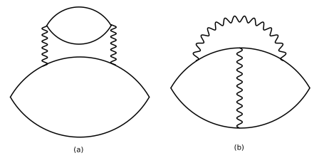
Figure S1: The Feynman diagrams representing the corrections to thermodynamic potential. (a) Hartree diagram. (b) Fock diagram.

According to the linked cluster theorem, the thermodynamical potential is reduced to the computation of closed Feynman diagrams. We employ perturbation theory in interactions and consider two leading diagrams depicted in Fig. (S1). The calculation presented here is for a single spin. The Hartree term, given by the diagram Fig. (S1)a, gives the following contribution to the potential

$$\Omega_{a}=-T\sum_{\nu_{m}}\Pi(i\nu_{m})\Pi(i\nu_{m}).$$ (S34)

Here $\nu_{m}=2\pi mT$. The Fock term, depicted in Fig. (S1)b, gives

$$\Omega_{b}=T^{3}\textbf{tr}\sum_{m,n,l}G(i\omega_{m})G(i\omega_{m}-\nu_{l})G(i\omega_{m}-\nu_{l}-i\nu_{n})G(i\omega_{m}-i\nu_{n}).$$ (S35)

V.1 Hartree diagram

Due to the chiral structure, the leading contribution to $\Omega_{a}$ is from the zero-momentum transfer. Upon summing over $\nu_{m}$ and defining dimensionless variable $x=2\pi Tr/v_{F}$, one obtains

$$\Omega_{a} = -vU^{2}T^{3}\frac{k_{F}^{2}}{\pi v_{F}^{4}}\int_{2\pi T/E_{F}}^{\infty}\frac{dx}{x}\frac{1}{(\sinh x)^{2}\tanh x}.$$ (S36)

The integral $\int_{2\pi T/E_{F}}^{\infty}\frac{dx}{x}\frac{1}{(\sinh x)^{2}\tanh x}=c_{0}(2\pi T/E_{F})^{-3}-c_{1}+O(T/E_{F})$. Here $c_{0}$ and $c_{1}$ are two constants. Importantly, one may write $c_{1}$ as a generic integral $c_{1}=\int_{0}^{\infty}\frac{dx}{x}\Big{[}\frac{1}{x^{3}}-\frac{1}{(\sinh x)^{2}\tanh x}\Big{]}$ Numerically, it is approximately given by $c_{1}\approx 0.121727$. Then we consider the specific heat per unit volume

$$C^{a}_{v}=\frac{1}{v}\frac{\partial\Omega_{a}}{\partial T}\Big{|}_{v}.$$ (S37)

Obviously, the leading contribution comes from the $\propto c_{1}$ part. Thus we obtain

$$C^{a}_{v}=3c\Big{(}\frac{k_{F}U}{v_{F}}\Big{)}^{2}\frac{T^{2}}{\pi v_{F}^{2}}.$$ (S38)

This $T^{2}$ behavior is a typical property of 2D Fermi-liquids.

V.2 Fock diagram

Upon the summation over $m,n,l$ in Eq. (S35), we obtain the following integral expression

$$\Omega_{b}=\frac{vT}{(2\pi)^{3}}\Big{(}\frac{k_{F}U}{v_{F}}\Big{)}^{2}\frac{\omega_{0}^{2}}{2v_{F}^{2}}\int^{+\infty}_{2\pi T/E_{F}}zdz\frac{1}{\sinh^{2}z\tanh z}.$$ (S39)

The integral $\int^{+\infty}_{2\pi T/E_{F}}zdz\frac{1}{\sinh^{2}z\tanh z}=a_{0}\frac{E_{F}}{T}-\frac{1}{2}+O(T^{3}/E^{3}_{F})$. Here $a_{0}$ is a constant. Thus its contribution to specific heat, $C^{b}_{v}$, now reads

$$C^{b}_{v}\simeq-\frac{1}{(2\pi)^{3}}\Big{(}\frac{k_{F}U}{v_{F}}\Big{)}^{2}\frac{\omega_{0}^{2}}{4v^{2}_{F}}.$$ (S40)

This is a constant correction to specific heat, which only depends on the magnetic field $B$, $v_{F}$, $k_{F}$ and the interaction strength $U_{0}$.

VI Zeeman effect

In this section, we argue that the Zeeman effect gives subleading corrections to thermodynamics compared to the (pseudo)-spin phase. The Zeeman effect originate from the coupling $-\frac{1}{2}\mu_{B}B1_{4}\otimes\hat{\alpha}_{z}.$ Here $\mu_{B}$ is the Bohr magneton and $\hat{\alpha}_{z}$ is the Pauli matrix acting on the (real-)spin of electron. Since energy is splitted by the Zeeman effect, each spin’s Fermi momentum is different. Namely,

$$k^{s}_{F}=k_{F}+\frac{s}{2}\frac{\mu_{B}B}{v_{F}},$$ (S41)

where $k_{F}$ is defined by $\epsilon_{F}/v_{F}$. We find that the propagator is modified to be $G_{K,s}(\mathbf{r},\delta w)\approx\frac{I_{s}}{2}\Big{(}1+(\text{sgn}(\omega)+\frac{i}{2k^{s}_{F}r})\hat{r}\cdot\hat{\sigma}\Big{)}$. Two observations: (1) The chiraly feature is not influenced by the Zeeman effect. (2) $k^{s}_{F}$ enters the oscillatory function. This is the key point to consider the Zeeman effect. In fact, it affects the thermodynamic potential in the following way

$$\Omega^{z}_{a}=-TU^{2}_{2k_{F}}\sum_{\nu_{m}}\int d^{2}r\Pi_{+}(i\nu_{m},r)\Pi_{-}(i\nu_{m},r).$$ (S42)

Here $\Omega^{z}_{a}$ is the correction to the thermodynamic potential by Zeeman effect and $\Pi_{\pm}$ is $2k_{F}$ polarization operator for spin up and down respectively. Here $\Pi_{2k_{F}}^{s}$ is the $2k_{F}$ polarization operator for the spin-up/down $(s=+/-)$ electron. However, in Graphene, the $2k_{F}$-scattering is suppressed by chirality. In fact, $\Pi_{2k_{F}}^{+}(r)\Pi_{2k_{F}}^{-}(r)$ carries one extra decaying factor $(k_{F}r)^{-2}$. Since the characteristic scale for $r$ is the thermal length $v_{F}/T$, the decaying factor then translates into a small factor, $T^{2}/E_{F}^{2}$.

In the Zeeman effect, the fundamental energy scale is $\omega_{z}=\mu_{B}B$. Set $B=x(T)$ and then $\omega_{z}$ given by

$$\omega_{z}=9.27x\times 10^{-24}J.$$ (S43)

The effective cyclotron-frequency is given by $\omega_{0}=\hbar v_{F}/R_{L}$. If $k^{-1}_{F}\simeq 1.65$ nm, the Larmor radius given by $R_{L}\simeq\frac{400}{x}nm=4\times 10^{-7}/x(m)$. For simplicity, we take $v_{F}=10^{6}m/s$. Recall $\hbar\simeq 10^{-34}J\cdot s$. Then the energy scale $\omega_{0}$ is estimated by

$$\omega_{0}=\frac{x}{4}\times 10^{-21}J.$$ (S44)

It is easy to see that $\omega_{0}\gg\omega_{z}$.

From smallness of $T^{2}/E_{F}^{2}$ and $\omega_{z}/\omega_{0}$, one observes that the Zeeman effect gives parametrically smaller corrections compared to the effect coming from the pseudospin-dependent orbital phase.

VII Effect of curving of the electron trajectory

In this section, we consider the effect of curving of the electron trajectory and argue that it gives a sub-leading correction to the thermodynamic characteristics of the interacting electron gas. Curving of the trajectory manifests itself in the two-loop diagram in the RPA sequence. Now we consider the correction to DOS and find that it is proportional to the following expression

$$P(\mathbf{r},\omega)=U^{2}_{2k_{F}}u_{0}^{2}\text{tr}\int d^{2}r_{1}d^{2}r_{2}G(\mathbf{r},\mathbf{r}_{1};\omega)G(\mathbf{r}_{1},\mathbf{r}_{2};\omega)G(\mathbf{r}_{2},\mathbf{r};\omega)\Pi(\mathbf{r}_{1};0)\Pi(\mathbf{r}_{2};0),$$ (S45)

where $U_{2k_{F}}$ is the $2k_{F}$ component of interaction and $u_{0}$ is the strength of the point-like impurity. Since we focus on the effect trajectory, we only preserve the $p_{0}^{3}r^{3}$-corrections and ignore the spin-dependent phase correction in $P$. We call this part as $P_{0}$, given by the following integral expression

$$P_{0}= -\frac{\partial_{\omega}}{2}\text{tr}\int d^{2}r_{1}d^{2}r_{2}\frac{1}{2\pi v_{F}^{2}|\mathbf{r}_{1}-\mathbf{r}_{2}|^{2}}\exp 2i\left((k_{F}+\frac{\omega}{v_{F}})|\mathbf{r}_{1}-\mathbf{r}_{2}|-\frac{p_{0}^{3}|\mathbf{r}_{1}-\mathbf{r}_{2}|^{3}}{24}\right)$$ (S46)

$$\times\frac{1}{4\pi^{2}v_{F}r_{1}^{3}}\cos(2k_{F}r_{1}-\frac{p^{3}_{0}r_{1}^{3}}{12})\times\frac{1}{4\pi^{2}v_{F}r_{2}^{3}}\cos(2k_{F}r_{2}-\frac{p^{3}_{0}r_{2}^{3}}{12})U^{2}_{2k_{F}}u_{0}^{2}.$$

In the exponential, the main oscillating term is $2k_{F}|\mathbf{r}_{1}-\mathbf{r}_{2}|\pm 2k_{F}r_{1}\pm 2k_{F}r_{2}$. We only need the slowly oscillatory piece. Namely, we want $2k_{F}|\mathbf{r}_{1}-\mathbf{r}_{2}|\pm 2k_{F}r_{1}\pm 2k_{F}r_{2}\simeq 0$. This demands that $\mathbf{0},\mathbf{r}_{1},\mathbf{r}_{2}$ are aligned in a straight line. For simplicity, we take $\mathbf{r}_{1}/r_{1}\simeq-\mathbf{r}_{2}/r_{2}$. Use the expression $|\mathbf{r}_{1}-\mathbf{r}_{2}|=|r_{1}+r_{2}|\sqrt{1-\frac{2r_{1}r_{2}}{|r_{1}+r_{2}|}(1+\cos\theta)}$ where $\theta$ is the angle bewteen $\mathbf{r}_{1}$ and $\mathbf{r}_{2}$. If $\theta\simeq\pi$, then $|\mathbf{r}_{1}-\mathbf{r}_{2}|\simeq r_{1}+r_{2}+\frac{r_{1}r_{2}}{2|r_{1}+r_{2}|}(\theta-\pi)^{2}$. Then the integral over $\theta$ introduces extra factor, shown as below

$$\int_{\theta\sim\pi}d\theta\exp(ik_{F}\frac{r_{1}r_{2}}{|r_{1}+r_{2}|}(\theta-\pi)^{2})\approx e^{i\pi/4}\sqrt{\frac{\pi|r_{1}+r_{2}|}{k_{F}r_{1}r_{2}}}.$$ (S47)

We only trace the field-dependent correction, by considering $\delta P_{0}^{a}(B)=P_{0}^{a}(B)-P_{0}^{a}(0)$. Further we do the following variable change: $x=p_{0}r_{1}$ and $y=p_{0}r_{2}$. Here $x$ and $y$ are both dimensionless. Then $\delta P_{0}^{a}$ is given by $U^{2}_{2k_{F}}u_{0}^{2}v_{F}^{5}k_{F}^{-1/2}p_{0}^{-7/2}F_{\Gamma}(\omega/\epsilon_{0})$ and $F_{\Gamma}$ is given by

$$F_{\Gamma} \equiv -i\int_{x,y>\Gamma}dxdy\left[\exp 2i\left(\frac{\omega}{\epsilon_{0}}(x+y)-\frac{\left[x^{2}y+xy^{2}\right]}{8}\right)-\exp 2i\left(\frac{\omega}{\epsilon_{0}}(x+y)\right)\right]$$ (S48)

$$\times\frac{1}{4\pi^{2}x^{2}}\times\frac{1}{4\pi^{2}y^{2}}\times e^{i\pi/4}\sqrt{\frac{\pi}{xy(x+y)}},$$

where $\Gamma\ll 1$ is small cut-off with order of $p_{0}/k_{F}$ and $\epsilon_{0}=v_{F}p_{0}$. Numerically, we trace the $\Gamma$-independent term, namely $F(\omega/\epsilon_{0})$, in Eq. S48 and find that $F(\omega/\epsilon_{0})$ is smooth function of $\omega/\epsilon$ and has the amplitude that is smaller than $1$. Thus, we conclude that the curved trajectory give a correction to the DOS with a coefficient, $\propto B^{7/2}$. Since we consider a weak magnetic field, the $B^{7/2}$ is obviously the high order perturbation relative to $B^{2}$. Further, $F(\omega/\epsilon_{0})$ is smooth and smaller than $1$, while $E^{2}_{F}/\omega^{2}$ is large. Thus the effect of curved trajectory gives the sub-leading corrections.