Measuring the magnetic origins of solar flares, CMEs and Space Weather

Abstract

We take a broad look at the problem of identifying the magnetic solar causes of space weather. With the lackluster performance of extrapolations based upon magnetic field measurements in the photosphere, we identify a region in the near UV part of the spectrum as optimal for studying the development of magnetic free energy over active regions. Using data from SORCE, Hubble Space Telescope, and SKYLAB, along with 1D computations of the near-UV (NUV) spectrum and numerical experiments based on the MURaM radiation-MHD and HanleRT radiative transfer codes, we address multiple challenges. These challenges are best met through a combination of near UV lines of bright Mg II, and lines of Fe II and Fe I (mostly within the $4s-4p$ transition array) which form in the chromosphere up to $2\times 10^{4}$ K. Both Hanle and Zeeman effects can in principle be used to derive vector magnetic fields. However, for any given spectral line the $\tau=1$ surfaces are generally geometrically corrugated owing to fine structure such as fibrils and spicules. By using multiple spectral lines spanning different optical depths, magnetic fields across nearly-horizontal surfaces can be inferred in regions of low plasma $\beta$, from which free energies, magnetic topology and other quantities can be derived.

Based upon the recently-reported successful suborbital space measurements of magnetic fields with the CLASP2 instrument, we argue that a modest space-borne telescope will be able to make significant advances in the attempts to predict solar eruptions. Difficulties associated with blended lines are shown to be minor in an Appendix.

1 Introduction

Commenting on the origin of solar flares, in 1960 Gold & Hoyle wrote

The requirements of the theory can therefore be stated quite definitely. Magnetic field configurations must be found that are capable of storing energy densities hundreds of times greater than occur in any other form, and that are stable most of the time. A situation that occurs only a small fraction of the time must be able to lead to instability in which this energy can rapidly be dissipated into heat and mass motion…

These requirements have remained unchanged in the intervening six decades. We now have a “standard model” of flares (Carmichael, 1964; Sturrock, 1966; Hirayama, 1974; Kopp & Pneuman, 1976), involving a loss of equilibrium of arcades of closed magnetic flux systems, particle acceleration and, frequently, ejection of plasmoids. The instability can only arise when the free magnetic energy stored in the coronal magnetic fields exceeds certain thresholds. This is, however, a necessary but not sufficient condition for flaring and plasmoid ejection, because other global and local properties of the magnetic field, notably the topology, also determine the stabilility of coronal MHD systems (Low, 1994).

Enormous interest in solar eruptions is driven by society’s need to understand origins of “space weather” (e.g. Eddy, 2009) as well as its intrinsic scientific challenges. However, much like weather prediction before the advent of modern instrumentation and computers, predicting the properties of eruptions and flares has remained a difficult challenge primarily due to the lack of quantitative data available for analysis of the pre-flare state and flare-triggering mechanism(s). In particular, the only high-resolution, high cadence, data available to date has been the magnetic field state in the photosphere, which has been used to define “boundary conditions” to the overlying coronal magnetic field, where most of the free energy is stored prior to eruption. Herein lies the basic problem: magnetic fields measured in the photosphere are not ideally suited to the task. We elaborate upon this below.

The situation described by Gold & Hoyle (1960) draws analogy with trying to predict the timing and location of lightning strikes (Judge, 2020). By measuring updrafts and/or observing cloud buildup one can identify the causes of the buildup of electrostatic energy, but lightning occurs in a predictable way only in a statistical sense. In-situ measurements of electric fields are required even then to make probabilistic forecasts of lightning strikes to the ground, without reference to intra- or inter- cloud discharges. In this sense the weaknesses found in previous prediction methods is perhaps unsurprising.

The difficulty of the task has been summarized in the write-up of an inter-agency “All Clear Workshop” (Barnes et al., 2016) in which the authors conclude with the sobering statement that

For M-class flares and above, the set of methods tends toward a weakly positive skill score (as measured with several distinct metrics), with no participating method proving substantially better than climatological forecasts.

Steady improvements in the performance of flare forecasts has been documented in more recent years (e.g. Leka et al., 2019). However, these authors make explicit the need to augment existing photospheric magnetic data in order to proceed, with a heterogeneous mix of theory and observation:

quantitative “modern” forecasts incorporate …physical understanding as they often characterize coronal magnetic energy storage by proxy, with the parameterizations of photospheric magnetograms.

In other words, measurements of the photospheric magnetic field can be related only indirectly and through certain ad-hoc parameterizations, to the magnetic free energy of the overlying corona, which is the ultimate origin of instabilities leading to flares and CMEs.

With the availability of a decade of high-resolution photospheric magnetic field data from NASA’s Solar Dynamics Observatory (SDO) mission, recent efforts have focused on statistical pattern recognition methods for flare prediction that generally fall under the “machine learning (ML)” sub-field of artificial intelligence research. For example, a study by Bobra & Couvidat (2015) used photospheric vector magnetic data of 2071 active regions from the Helioseismic and Magnetic Imager (HMI) instrument on SDO. They predicted strong flares using a Support Vector Machine (SVM) algorithm applied to a set of 25 parameters derived from the vector magnetic field measured in SHARPs (Space-weather HMI Active Region Patches), which are cut-outs around sunspot active regions. They achieved a high True Skill Statistic (TSS) of $\approx$ 0.8, but at the cost of getting a significant number of false positives, a common characteristic of all ML flare prediction algorithms optimized for TSS in the strongly unbalanced training sets which naturally contain many more “no flare” examples than “flare” examples. Later studies (Park et al., 2018; Liu et al., 2019; Chen et al., 2019; Li et al., 2020) applied recurrent architectures such as Long Short-Term Memory (LSTM) systems and deep learning systems including Convolution Neural Network (CNN) and autoencoder architectures to explore feature sets that extend beyond the magnetic field-derived features of earlier ML flare prediction systems. However these studies do not demonstrate significant increases in skill scores relative to earlier approaches.

These studies have used only photospheric measurements of magnetic fields. Investigations have also been carried out that include information from higher atmospheric layers, e.g., by incorporating SDO Atmospheric Imaging Array (AIA) data into existing ML flare prediction systems (Nishizuka et al., 2018; Jonas et al., 2018), or by using extrapolated coronal magnetic field models (Korsós et al., 2020). Chromospheric UV spectral lines from IRIS have also been scrutinized for additional flare prediction utility (Panos & Kleint, 2020). These studies all show some degree of improvement in flare prediction metrics when including chromospheric or derived coronal information. More recently, Deshmukh et al. (2020) showed that combining Topological Data Analysis (TDA) of the radial magnetic field structure in active regions with the SHARPs vector magnetic field metadata results in similar or slightly higher skill scores compared to using selected SHARPs metadata alone. This result implies that inclusion of high-resolution imaging of active region and flows may be an important complement to spectroscopic measurements when deducing atmospheric conditions that evolve to a flaring state.

Physically, however, solar flare prediction based upon photospheric data is ultimately confronted with basic difficulties, beyond the well-known disambiguation problem associated with native symmetries in the Zeeman effect. The photosphere is a dense radiating layer of high density ($10^{-7}$ g cm^-3) plasma. Outside of sunspot umbrae the photospheric magnetic field is unable to suppress convective motions which therefore control the magnetic fields threading the fluid, a case where the plasma-$\beta=$ gas pressure / magnetic pressure, is generally $>1$. In traversing the chromosphere, emerging magnetic fields drop in strength algebraically but the plasma densities and energy densities drop exponentially (by 7 and 5 orders of magnitude, respectively), so that the tenuous plasma at the coronal base is in a low-$\beta$ state. One immediate practical problem is that tiny dynamical changes which may be unobservable in the dense photosphere can have enormous consequences for the tenuous plasma and magnetic fields above: the problem is observationally ill-posed. As a result of these different photospheric and coronal plasma regimes, the time scales for significant photospheric magnetic field evolution are typically measured in minutes to hours whereas the dynamic evolution and reconnection of the coronal magnetic field configurations leading to flares, after a quasi-static buildup phase, is measured in seconds. This fundamental mismatch in dynamical time scales evidently cannot be overcome through any type of analysis of photospheric magnetic field data and leads to the conclusion that quantitative analysis of the magnetic field and flows in the chromosphere and corona are necessary to catalyze significant breakthroughs.

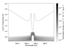
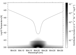
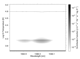
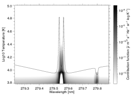
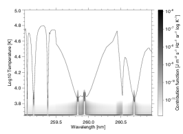
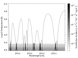
Figure 1: Contribution functions are shown as a function of temperature from the model C of Fontenla et al. (1993). The emergent intensities are over-plotted as solid lines for a ray from close to disk center ($\cos\theta=0.887$, $\theta$ the angular distance from disk center as measured from Sun center). The Ca II lines at 393 and 854 nm span from 3.8 to 4.0 in log$T$ (the latter forming in deeper cooler layers than the former), and the 1083 nm line of He I forms within the last pressure scale height of the chromosphere. Notice the extension of contributions for the Mg II resonance lines beyond all others, to $\log T_{e}\geq 4.3$, and the multiple lines of Fe II between 259 and 261 nm whose cores form close to 3.9-4.0 in log$T$, and weaker lines in the 275 nm region with stronger contributions from lower temperatures. A modest atomic model for Fe II was adopted to examine the line cores formed in non LTE in the upper chromosphere. The calculations used the RH computer program Uitenbroek (2001). Far more complete LTE calculations are made in the Appendix where spectral line blends are discussed.

In order to address this and other questions, our purpose here is to explore the entire solar spectrum to attempt to identify more direct ways to identify the free energy and topology of magnetic fields above active regions. In this way we hope to put the prediction of solar magnetic eruptions, the source of all major space weather events, on a firm observational basis. The specific problem we address is reviewed in section 2. It will involve spectro-polarimetry.

Before proceeding, we point out that our goals may on first reading appear similar to efforts measuring only intensities of EUV and UV emission lines (e.g. De Pontieu et al., 2020), an endeavor with a history of 6+ decades yet able to study only the effects and not causes of magnetic energy storage and release. Instead our work is closer to an important study by Trujillo Bueno et al. (2017), but the latter focuses more on the physical processes behind the magnetic imprints across the solar UV spectrum, including the near-UV spectral region of the Mg II $h$ & $k$ lines. We focus instead on finding an optimal set of observations which target the problem of the build-up and release of magnetic energy. We argue that spectro-polarimetry of the near-UV solar spectrum is indeed a profitable avenue for research.

2 Observational signatures of energy build-up and release

2.1 Measuring magnetic fields in and above chromospheric plasma

Two approaches are in principle possible: in-situ measurements and remote sensing. Clearly in-situ methods are far beyond the capabilities of known technology. The state-of-the-art mission Parker Solar Probe (Fox et al., 2016) has a perihelion distance of just below ten solar radii, far above active regions where most of the free magnetic energy exists. Therefore we limit our discussion to measuring magnetic fields remotely, an area which has a firm physical basis (Landi degl’Innocenti & Landolfi, 2004).

Briefly, two types of remote-sensing measurements have been made: direct measurements of light emitted from within coronal plasma, and measurements close to the corona’s lower boundary, some 9 pressure scale heights above the photosphere. Coronal measurements include (see, for example, reviews by Judge et al., 2001; Casini et al., 2017; Kleint & Gandorfer, 2017, for more complete references):

• Measurements of line-of-sight (LOS) field strengths using differences between ordinary and extraordinary rays of magneto-ionic theory at GHz frequencies Gelfreikh (1994).

• Measurements of field strengths across surfaces determined typically by a harmonic of gyro-resonant motions of electrons at frequencies of several GHz, frequencies uncontaminated by bremsstrahlung opacity only when the field strength exceeds $\approx$200 G (White, 2004).

• Serendipitous level-crossings in atomic ions produces changes in EUV spectra through level mixing by the Zeeman effect (Li et al., 2017), yielding magnetic field strengths.

• A long history of measurements of magnetic dipole lines during eclipses or with coronagraphs hold great promise for measuring vector magnetic fields in the corona. The infrared, coronagraphic DKIST facility offers significant new opportunities for advancements using such lines (e.g. Judge et al., 2013).

• Occultations of background radio sources by the corona have revealed integrated properties of coronal magnetic fields, weighted by electron density through the Faraday effect (Bird & Edenhofer, 1990), a technique also applied to signals from spacecraft away from the Sun-Earth line (Bird, 1982).

Of the second type, we can list:

• Several strong lines measured using spectro-polarimetric measurements of the Zeeman effect from the ground can yield LOS components of chromospheric magnetic fields. Very high photometric precision is however required for vector fields, beyond most current capabilities (Uitenbroek, 2010), owing to the second-order $\epsilon^{2}$ signature of the Zeeman effect in the small ratio $\epsilon$ of magnetic splitting to the line Doppler width (defined below). These include Na I D lines, Ca II H, K and infrared triplet lines. Synthetic Ca II line profiles are shown in the non-LTE calculations using the RH non-LTE program including partial redistribution (Uitenbroek, 2001) in Figure 1.

• The He I 1083 nm triplet has a proven record of magnetic field determinations in a variety of cool structures such as spicules (Centeno et al., 2010), filaments (Kuckein et al., 2012; Díaz Baso et al., 2019) and cool loops (Solanki et al., 2003), in the vicinity of the base of the corona before, during and after flares (Judge et al., 2014) even extending far into the corona (Judge et al., 2012; Schad et al., 2016). Both the Zeeman and Hanle effects contribute to the formation of this line, owing to the large contribution of anisotropic radiation incident on the helium atoms to the statistical equilibrium in the triplet states (e.g. Trujillo Bueno & Asensio Ramos, 2007).

• Recently, sub-orbital rockets have carried sensitive spectropolarimeters to observe the resonance lines of hydrogen (Kano et al., 2017) and singly-ionized magnesium (Trujillo Bueno et al., 2018; Ishikawa et al., 2021). Both Zeeman and Hanle effects have revealed information on magnetic fields near the very top of the solar chromosphere.

• Measurements at 30 GHz and above made with the ALMA interferometer facility can in principle yield line-of-sight magnetic field strengths using Gelfreikh’s (1994) theory of continuum polarization (Loukitcheva, 2014, 2020), but we have been unable to find reports of solar polarization measurements with ALMA. It can observe from 0.4 to 8.8 mm wavelengths (750 and 34 Ghz respectively), thereby sampling heights from 600 km to 2000 km in the chromosphere. Transition region plasma under non-flaring conditions is tenuous and thin. It contributes very little to the far brighter chromospheric emission at the high frequencies measured by ALMA.

Next we assess the ability of these techniques to address the specific problem of interest.

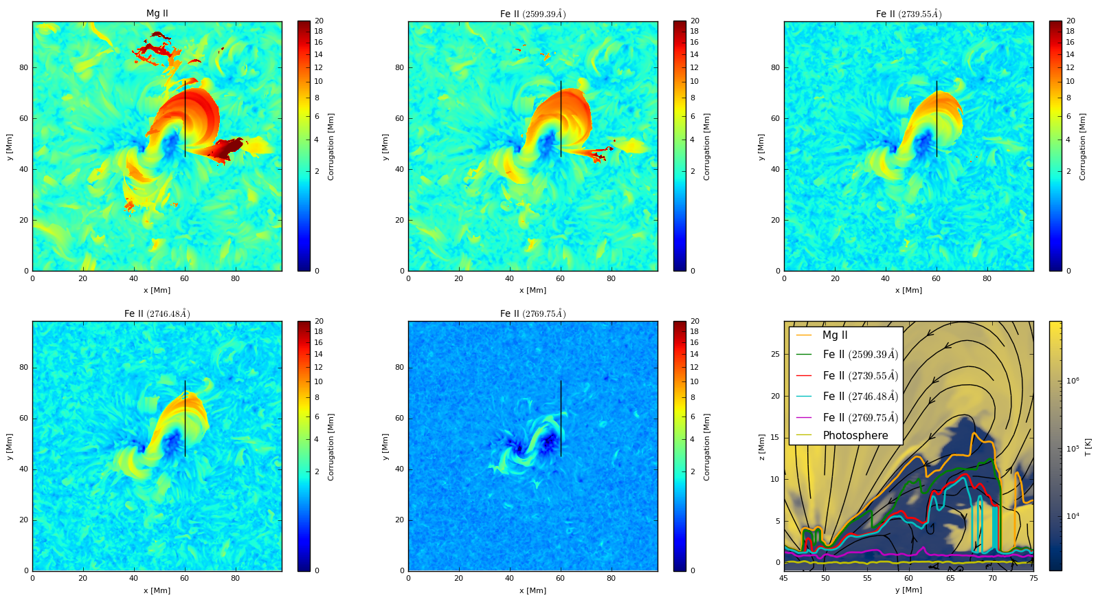
Figure 2: Images are shown to highlight the corrugated surfaces at which the centers of UV lines are formed (close to $\tau=1$) in MURaM calculations of the upper solar chromosphere. The calculations are from a numerical experiment where a magnetic flux system is emerging from beneath the solar atmosphere. The emergent fields carry with them plasma, which is revealed by the extended heights of the $\tau=1$ surfaces, which can exceed 10 Mm. Typically the line shifts in the lower transition region are smaller than the line widths (Athay & Dere, 1991). Therefore the $\tau=1$ surfaces were computed without taking into account Doppler shifts, at the centers of lines of Mg II $k$, and several lines of Fe II. The $x-y$ images of height of formation are plotted in order of decreasing opacity from Mg II to Fe II 2769.75 Å. In the bottom right panel, slices of these $\tau=1$ surfaces are shown, taken along the black line in the five other panels. But the black lines in this final panel are magnetic lines of force in the $y-z$ plane. Evidently, a combination of these and other lines of iron with a wide range of opacities spans the ranges of excursions of the surfaces away from a horizontal plane.

2.2 Establishing methods to measure free magnetic energy and topology

While information on magnetism above the photosphere is contained in all the above strategies, few offer ways to assess the necessary quantities concerning magnetic free energy as magnetic fields emerge, build and change topology as it evolves and is suddenly released. If we consider measurements within the corona, we would have to probe the 3D magnetic structure. However, the corona is optically thin (with the exception of gyro-resonance emission which yields just the magnetic field strength within resonant surfaces, whose geometry is not known from one line of sight), which means that recovery of the 3D coronal field would require measurements from at least two different lines of sight (e.g. Kramar et al., 2006). Until suitable instruments are flown on spacecraft away from the Sun-Earth line, the required stereoscopic views will be unavailable. Therefore we must seek alternatives.

When chromospheric, transition region and coronal plasmas are connected by magnetic lines of force (Judge, 2021), the plasma pressure near the top of the chromosphere is close to that of the overlying corona. Accurate measurements of magnetic fields using spectral lines formed in plasma up to a few times $10^{4}$ K can therefore be used to inform us on the evolving magnetic state of the overlying corona (Trujillo Bueno et al., 2017). Selected spectral line profiles formed across the upper chromosphere are shown in Figure 1, intended to illustrate near UV lines in comparison to familiar lines commonly observed from the ground. The solar spectrum between 250 and 281 nm is dominated by line transitions of Mg II and many lines belonging to the $4s-4p$ transition array in neutral and singly ionized iron. In the figure, contributions to the intensities of Mg II and typical Fe II lines are shown as a function of electron temperature. This abscissa was chosen instead of height and continuum optical depth because in the particular 1-dimensional model adopted, the temperature gradient in the transition region is very large, making lines appear to originate from the same heights.

The regime of plasma $\beta=8\pi p/B^{2}<1$ in upper chromospheric, transition region and coronal lines is the same, if the photospheric magnetic field has expanded to fill the volume. In active region plasma this appears to be the case (Ishikawa et al., 2021). When measurements are made close to the force-free state ($\beta\ll 1$), then theory can be reliably invoked in at least two ways: application of the magnetic virial theorem (Chandrasekhar, 1961), and extrapolation of fields with observational boundary conditions compatible with the magnetostatic conditions (Wiegelmann & Sakurai, 2021). Any waves and/or tangential discontinuities measured will also be of importance to assessing the free magnetic energy and its evolution. Fleishman et al. (2017) have confirmed these theoretical concepts quantitatively using model simulations.

Skeptics of our statements might rightfully recall that the chromosphere is finely structured (see, e.g., the remarkable structure in narrow-band images of Cauzzi et al., 2008; Wang et al., 2016; Robustini et al., 2018). It is also known, for example from limb observations, that transition region plasma at intermediate temperatures has contributions from structures far from a level surface which might otherwise be amenable to mathematical techniques to estimate free energies and extrapolated magnetic fields. A non-level, “corrugated” surface of unit optical depth in a given spectral line can lead to spurious inferences of magnetic structure even within low-$\beta$ plasmas (see, e.g., section 4.3 of the paper by Trujillo Bueno et al., 2017, and our Figure 2 below). The question then arises, is the interface between chromosphere and corona just too finely structured to make measurements of magnetic fields there of little use?

Hints from two pieces of work suggest that this is not the case. Firstly, the CLASP2 measurements reported by Ishikawa et al. (2021) have shown that, at an angular resolution of 1” which is far smaller than the scales of large coronal structures leading to flares, the fields measured in the core of the Mg II $h$ & $k$ lines across active regions are unipolar and spatially smooth over large areas. Any mixed polarity fields undetected by CLASP2 must lie below 1” scales and will therefore not penetrate more than a few hundred km above the photosphere. But the fields measured by CLASP2 may well contain unseen tangential discontinuities arising from small-scale angular displacements across flux surfaces (Judge et al., 2011). Such features would constitute an additional source of free magnetic energy whose consequences might then be explored using the very techniques advocated for below. Secondly, Judge (2021) has shown that the attention to the dynamics and fine structure of transition region plasma has been over-emphasized, statistically. Most of the chromosphere-corona transition region on the Sun is indeed in a thermal interface connected by magnetic lines of force, and not isolated, as was claimed by Hansteen et al. (2014) and references therein, all of them based on circumstantial evidence accumulated using spectral line intensities alone.

One example is shown in Figure 2. This figure is based on a MURaM flux emergence simulation in a 98 Mm wide domain, reaching from -8 to 75 Mm in the vertical direction. The snapshot corresponds to a highly energized corona, in which a strong bipolar field has emerged into a previously quiet region. Ten minutes after this, a flare and a mass ejection occurred. The simulation is based on the Rempel (2017) version of MURaM, which uses a simplified description of the chromosphere. The $\tau=1$ surfaces were computed using parameterized li¡ne opacities at line center and integrating downwards from the corona. The opacities were derived using a function, which for the Mg II $k$-line for example, are of the form

$$\kappa_{\nu=\nu_{0}}=\frac{\pi e^{2}f_{ij}}{m_{e}c}\frac{n_{\mathrm{i}}}{n_{\mathrm{Mg^{+}}}}\frac{n_{\mathrm{Mg}^{+}}}{n_{\mathrm{Mg}}}\frac{n_{\mathrm{Mg}}}{n_{\mathrm{H}}}n_{\mathrm{H}}\phi_{\nu_{0}},$$ (1)

in which the lower level population $n_{\mathrm{i}}$ is expanded as a product of ionization fraction $\frac{n_{\mathrm{Mg}^{+}}}{n_{\mathrm{Mg}}}$ (a function of electron temperature $T_{e}$), the abundance $\frac{n_{\mathrm{Mg}}}{n_{\mathrm{H}}}$, and the hydrogen density $n_{\mathrm{H}}$ from the model. The first factor is the frequency-integrated cross section of the $k$ line from fundamental constants and the absorption oscillator strength $f_{ij}$ between levels $i$ and $j$, and $\phi_{\nu}$ the line profile at frequency $\nu$, normalized so that $\int_{0}^{\infty}\phi_{\nu}d\nu=1$. The profile is dominated for these ions by an assumed microturbulence of 10 km s^-1. The term $\frac{n_{\mathrm{Mg}^{+}}}{n_{\mathrm{Mg}}}$ is computed assuming that neutral Mg is negligible, but allowing for electron impact ionization to Mg²⁺ and higher ions and radiative recombination using data from Allen (1973).

This figure illustrates approximate line formation heights, sufficient for the present paper. The excursions in height corresponding to the emerging flux system vary from a maximum near 10 Mm for Mg II $k$, to a few Mm for a line of Fe II at 276.9 nm. As can be seen, these corrugations can be probed with multiple spectral features with different opacities. Thus measurements at the top of the chromosphere, properly sampling the potential excursions of the isotherms and isobars in the transition between chromosphere and corona, appear to be a promising approach to the problem. At the very least, such new magnetic measurements could be compared in detail with advanced simulations of the Sun’s atmosphere (Gudiksen et al., 2011; Rempel, 2017). Below we will suggest one approach to this problem based upon machine learning techniques.

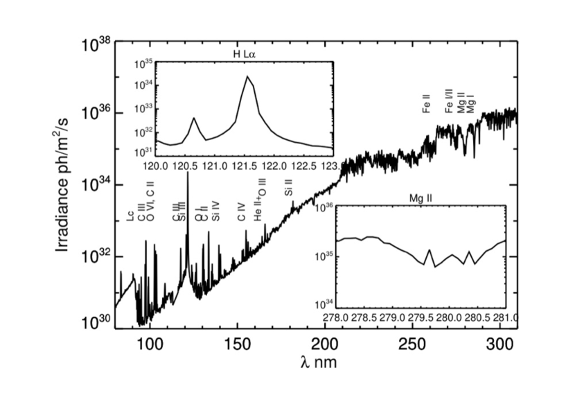
Figure 3: A low-resolution UV irradiance spectrum from the Whole Heliospheric Interval in 2008 is shown (from https://lasp.colorado.edu/lisird/data/whi_ref_spectra). The near UV region has a photon flux density far higher than the majority of vacuum UV lines below 200 nm. The exception is H L$\alpha$ which roughly 10x smaller than the flux density at 260 nm and longer wavelengths.

2.3 The near UV solar spectrum and the chromosphere-corona interface

A standard, low resolution solar UV spectrum is shown in Figure 3. After an extensive search, we have identified a spectral range of 256-281 nm as a promising part of the solar spectrum for measurement of vector magnetic fields at the base of the corona. Our search, driven by the need to probe in detail magnetic structure in height above the solar surface and/or depth along the LOS of prominences, led to the choice of important transitions in the 4s-4p transition array of Fe II. While there are strong Fe II 4s-4p transitions in the region near 234 nm, the solar fluxes are weaker than in the 256-281 nm range. Our wavelength selection is significantly broader than the 279.2-280.7 nm spectral region of CLASP2, which includes the Mg II $h$ & $k$ line cores and magnetically-sensitive wings (Auer et al., 1980; Belluzzi & Trujillo Bueno, 2012; Alsina Ballester et al., 2016; del Pino Alemán et al., 2016) the 3p-3d lines (del Pino Alemán et al., 2020), and photospheric lines of Mn I (Ishikawa et al., 2021). Both Hanle and Zeeman effects can be brought to bear on the problem depending on the strength of the magnetic fields found across the solar atmosphere. The Hanle effect can be important to remove the 180^o ambiguity present in Zeeman effect measurements. The rationale for this spectral region is based upon requirements demanded by the desire to measure vector magnetic fields within force-free ($\approx$ low $\beta$) plasma at the coronal base, over an area covering a typical active region. An angular resolution sufficient to resolve the thermodynamic fine structure is also a constraint. Such features are most clearly seen only in images of features within the narrow spectral lines chromospheric images. This constraint poses difficulties for current observations at radio and sub-mm wavelengths, and in hard X-rays. Soft X-rays ($\leq 1$ keV) have no known sensitivity to magnetic fields of solar magnitude, and along with EUV photons cannot escape from or penetrate deep into the chromosphere. We are then left to consider vacuum UV to infrared wavelengths.

We further eliminate wavelengths above the atmospheric cutoff at 310 nm because of the lack of spectral lines that can span many decades in optical depths above the chromosphere. The Balmer and higher line series of hydrogen are poor choices for Zeeman diagnostic work, the lightness of hydrogen makes lines broad and patterns overlapping. For Ba-$\alpha$, seven anomalous Zeeman patterns will lie within half a wave number for typical solar field strengths even in the photosphere, thereby making the observation of anomalous Zeeman patterns extremely difficult. The Hanle effect has been explored by Štěpán & Trujillo Bueno (2010) in their comparison of 1D radiative transfer calculations with limb observations of the quiet Sun by Gandorfer (2000). The value of H$\alpha$ as a diagnostic of magnetic field remains a subject for further research.

The strongest line in the chromospheric visible spectrum is Ca II $K$ has just $1/20$ the opacity of the Mg II $k$ line (see Figures 1 and 5). Also shown in Figure 1 is the well-known line of He I at 1083 nm which is present in active region plasma. However, the line, belonging to the triplet system, populated largely by recombination following EUV photoionization, tends to form where coronal ionizing photons (and perhaps even hot particles) cannot penetrate the chromosphere. Our non-LTE calculations (Figure 1) reveal that significant opacity in the line is narrowly confined between surfaces of column mass well below the height of the NUV Mg II lines, because of the depth of penetration of vacuum UV radiation from the overlying corona in the continua of H and He. When included along with the Ca II resonance and infrared triplet lines, the optical- near UV regions accessible from the ground extend neither high enough, nor do they sample opacity with the fineness of UV lines (Figures  1, 2 and 5. Lines of Mn I are sufficiently close to the strong Mg II lines for the wings of the latter to contribute to opacity, but this was not accounted for in the plot. Therefore heights of formation of Mn I lines are lower limits. ).

The solar irradiance spectrum at vacuum UV wavelengths (below 200 nm, and above 91 nm below which the Lyman continuum absorbs line radiation), including H L$\alpha$ and many chromospheric and transition region lines, is shown in Figure 3. All are substantially weaker than the Mg II lines. The polarimetric measurements necessary to infer magnetic fields require large photon fluxes. The VUV region is a factor of at least 10-100 times dimmer than the NUV. Also, the Zeeman signatures vary in proportion to the wavelengths observed. Further, most of the transition region lines are optically thin, so that there is no single “depth of formation” of a given line. The exceptions are the Lyman lines of hydrogen and 58.4 nm resonance line of He I. But using only this region of the spectrum would also fail to sample surfaces of multiple optical depths, and thus fail to address the need to span the anticipated corrugated isothermal and isobaric surfaces (Figure 2), particularly in active regions, the sources of most solar eruptions.

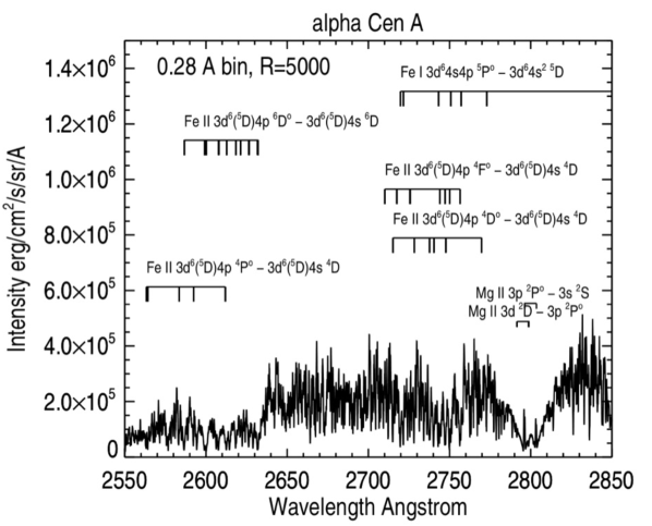
Figure 4: A smoothed UV spectrum of $\alpha$ Cen A, obtained by the Hubble Space Telescope, is displayed as a proxy for the mean solar intensity spectrum. The large number of lines of Fe I and Fe II are indicated and annotated with their multiplet terms. The Mg II spectrum is also annotated including the $3s-3p$ $h$ and $k$ lines, and the $3p-3d$ lines. Notice that the permitted Fe II lines (shown with solid bars with downward ticks) consist of the sextet-D resonance lines $(4s-4p)$ near 2600 Å, and quartet transitions at other wavelengths that occur between metastable (even parity) quartet lower levels and odd-parity quartets of the same transition array ($4s-4p)$.

In contrast, the NUV region (from say 200 to 310 nm, the atmospheric cutoff) is comparatively brighter, containing lines (Mg II) whose cores form within lower transition region. Compared with lines accessible from the ground, lines have smaller Zeeman signatures, but have increased linear polarization generated by the higher radiation anisotropies at UV wavelengths (much stronger limb-darkening). Thus, the Hanle signals will statistically be stronger than at visible wavelengths. Further, the region contains a plethora of lines of neutral and singly ionized iron within the $4s-4p$ transition array, including resonance lines near 260 nm (see Figure 4). Their complex spectra span and sample multiple depths across the chromosphere, extending into lower transition region plasma (see in particular the contours of unit optical depth surfaces for several lines in the lower right panel of Figure 2, and the plot of relative optical depths in Figure 5).

The richness of the Fe II spectrum itself has been known for decades in astronomy (e.g. Viotti et al., 1988). Figure 4 identifies lines and multiplets of Fe plotted above a smoothed Hubble Space Telescope spectrum of $\alpha$ Cen A, which is a good proxy for disk-averaged intensity spectrum of the Sun. (There is no disk-averaged solar spectrum of comparable quality). All of the strong transitions of iron lie near or below the Mg II lines near 280 nm. NUV spectra obtained at the solar limb during the SKYLAB era revealed a spectacular array of Fe II lines in emission against the darkness of space (Doschek et al., 1977). Particularly strong in the limb spectra (Figure 10) are multiplets in the sextet system near 259-263 nm, and quartet transitions in the 273 nm region. These Fe II lines were readily detected up to 8” above the limb in the SKYLAB data, the limb itself is already far higher than the photosphere. Such emission is very likely associated with the kind of structures modeled in Figure 2. A downside of the richness of the spectra of iron is the possibility of blended lines. The important issues of blended spectra lines at NUV wavelengths and effects of missing opacity are addressed in the Appendix. They are shown to be a minor issue, affecting only a few lines in the regions between 256 and 281 nm, owing to the overwhelming strength of the Fe II lines formed high enough in the chromosphere to aid in the diagnosis of magnetism there. Between 281 and 310 nm, there are just 10 “wide” lines, i.e. strong enough to exhibit wing absorption profiles, compared with 38 listed by Moore et al. (1982) between 256 and 281 nm. None of the lines above 281 nm form high enough in the Sun’s atmosphere to contribute significantly beyond measurements of the chromospheric magnetic field at shorter wavelengths.

Figure 5: Properties of spectral lines calculated using line center opacities as a function of wavelength are shown. Circles show lines of singly-charged ions, squares show lines of neutral species. Symbol sizes reflect critical Hanle field strengths. Relative optical depths of the lines are shown on the ordinate. The Mn I lines should include wing opacity from the Mg II line, but this was omitted here. The Mn I optical depths are thus a lower limit. The “?” for the He I 1083 nm line refers to the unknown relative optical depth of this line because of peculiarities in the formation of this multiplet in the Sun (e.g. Judge et al., 2015, who discuss this multiplet in the context of a well-observed flare).

Relative optical depths at the centers of the lines in this region, and “Hanle field strengths” are shown in Figure 5, including lines of He, Mg, Ca, Mn and Fe. These Hanle field strengths (see equations 2 and 3 below) are those near which the emergent polarized spectra are strongly sensitive to magnetic field strength and direction, (Landi degl’Innocenti & Landolfi, 2004, see below).

2.4 Spectral signatures of magnetic fields

The Zeeman effect is well-known in laboratory and astrophysics as a characteristic splitting in intensity ($I$) spectra. But in the Sun and stars, the Stokes parameters $I,Q,U$ and $V$ are used to measure magnetic fields in commonly encountered situations where the widths of the lines exceed the Zeeman splitting (this is assumed in the following discussion). As noted above, Zeeman signals depend upon the quantity $\varepsilon=\omega_{B}/\Delta\omega_{0}$, where $\omega_{B}$ is the Larmor frequency of the gyrating ion:

$$\hbar\omega_{B}=\mu_{0}B.$$ (2)

Here $\mu_{0}$ is the Bohr magneton, and $B$ the magnetic field strength in G. $\Delta\omega_{0}$ is the line width (Doppler width for chromospheric and coronal lines). The amplitude of circular polarization measured by Stokes $V$ varies linearly with $\epsilon$, the linear polarization profiles $Q$ and $U$ have amplitudes varying as $\varepsilon^{2}$. While $B$ is measured in Gauss, it is important to remember that unless contributions from non-magnetic regions to $I,Q,U$ and $V$ can be determined, the polarized components can be used to determine only the average flux density per unit area in Mx cm^-2, not field strength.

Table 1: Prominent lines and blends in the solar chromospheric spectrum

$\lambda$ nm	Landé g	log $\omega_{L}$	log $\sum_{i}A_{ji}$	$B_{HANLE}$	log $\tau_{0}$	Ion	blend
lab. (air)	factor	rad sec-1	sec-1	G			severity∗ Ion $\lambda$
256.254	1.21	7.03	8.49	28.8	-2.54	Fe II
256.348	1.10	6.99	8.49	31.9	-2.87	Fe II	1 Fe I .341
256.691	0.83	6.86	8.49	42.2	-3.30	Fe II
257.437	1.30	7.06	8.51	28.4	-4.33	Fe II	1 Co I .351
257.792	1.33	7.07	8.49	26.4	-3.32	Fe II	1 Mg I .888
258.258	1.47	7.11	8.49	23.9	-3.19	Fe II
258.588	1.50	7.12	8.46	21.7	-2.03	Fe II	2 Fe I .588
259.055	1.50	7.12	8.48	22.8	-4.47	Fe II	1 Co I .059
259.154	1.49	7.12	8.49	23.5	-3.24	Fe II
259.373	2.17	7.28	8.49	16.2	-4.02	Fe II	1 Mn I .372
259.837	1.50	7.12	8.46	21.7	-1.93	Fe II
259.940	1.56	7.14	8.46	21.1	-1.39	Fe II	1 Fe I .957
260.709	1.50	7.12	8.66	34.8	-1.99	Fe II
261.107	1.90	7.22	8.49	18.4	-4.23	Fe II	1 Cr II? .104
261.187	1.59	7.15	8.46	20.5	-1.79	Fe II
261.382	1.50	7.12	8.46	21.7	-2.20	Fe II
261.762	1.66	7.16	8.46	19.6	-2.36	Fe II
262.041	1.87	7.22	8.66	27.9	-3.75	Fe II
262.167	3.34	7.47	8.46	9.8	-2.76	Fe II
262.567	1.50	7.12	8.46	21.9	-2.08	Fe II
262.829	1.50	7.12	8.66	34.8	-2.21	Fe II
263.105	1.50	7.12	8.46	21.7	-2.02	Fe II	1 Fe II .045†
263.132	1.50	7.12	8.46	21.7	-1.97	Fe II
264.112	1.87	7.22	8.51	19.8	-4.62	Fe II	1 Ti I .089
268.351	1.84	7.21	8.51	20.1	-4.99	Fe II	2 Cr II .345
269.283	1.93	7.23	8.47	17.2	-4.40	Fe II	1 Fe I .265, Fe II .260
270.938	2.10	7.27	8.47	15.8	-4.30	Fe II	1 Cr II .931
271.441	1.50	7.12	8.60	30.3	-3.09	Fe II
271.670	1.33	7.07	8.46	24.8	-3.11	Fe II	1 Mn II .680
271.903	1.25	7.04	8.25	16.3	-4.45	Fe I	2 Fe I .903
272.090	1.17	7.01	8.28	18.4	-4.76	Fe I
272.358	1.00	6.94	8.27	21.1	-5.22	Fe I
272.488	1.20	7.02	8.47	27.7	-3.05	Fe II	1 Fe I .495
272.754	1.50	7.12	8.60	30.4	-3.05	Fe II
273.073	0.80	6.85	8.47	41.6	-3.19	Fe II
273.245	1.45	7.10	8.46	22.8	-4.92	Fe II	1 Fe II .233
273.697	1.50	7.12	8.60	30.3	-3.22	Fe II	1 Fe I .696
273.731	2.00	7.25	8.27	10.5	-5.12	Fe I
273.955	1.43	7.10	8.61	32.1	-2.31	Fe II
274.241	1.67	7.17	8.28	12.9	-5.01	Fe I	1 Ti I .230, V II .243
274.320	0.50	6.64	8.47	66.6	-2.81	Fe II
274.407	2.50	7.34	8.27	8.4	-5.51	Fe I
274.648	0.90	6.90	8.47	37.0	-2.59	Fe II
274.698	1.37	7.08	8.60	33.2	-2.66	Fe II	1 Fe I .698
274.918	1.20	7.02	8.60	38.0	-3.02	Fe II
274.932	1.07	6.97	8.46	30.9	-2.38	Fe II
274.949	0.00	4.31	8.60	…	-3.24	Fe II
275.014	1.58	7.14	8.25	12.8	-5.04	Fe I
275.574	1.17	7.01	8.46	28.1	-2.17	Fe II
275.633	2.00	7.25	8.28	10.7	-5.52	Fe I	2 Fe I .633, Cr II .630
276.181	1.50	7.12	8.60	30.4	-3.25	Fe II	1 Fe I .178, Cr I .174
276.893	1.50	7.12	8.60	30.3	-3.08	Fe II
277.273	1.50	7.12	8.61	30.6	-3.14	Fe II	1 Fe I .283
277.534	1.34	7.07	8.46	24.2	-6.06	Fe II	1 ?
279.565	1.17	7.01	8.43	25.3	0.00	Mg II
279.482	1.98	7.24	8.57	21.3	-5.65	Mn I
279.827	1.70	7.17	8.57	24.8	-5.79	Mn I
280.108	0.84	6.87	8.57	50.3	-5.96	Mn I
280.270	1.33	7.07	8.43	21.9	-0.30	Mg II
285.213	1.00	6.94	8.69	55.8	-2.20	Mg I
393.366	1.17	7.01	8.17	14.3	-1.55	Ca II
854.200	1.10	6.99	7.00	1.0	-2.50	Ca II

Landé g-factors are computed using LS coupling. The final column lists the severity of the blend (as assessed by Moore et al., 1982), and the wavelength of the blended line (decimal nm). ^∗The severity is: 0=unblended; 1=moderate blend; 2=severe blend. The data in Figure 5 are taken directly from this table. ^†The strong line of Fe II multiplet 1 is blended with a line of multiplet 171.

The Hanle effect has a quite different and complementary behavior independent of the Doppler width $\Delta\omega_{0}$. It requires a pre-existing state of polarization induced by symmetry breaking effects such as anisotropic and/or polarized incident radiation. When the radiation is anisotropic, such as radiation emerging into the upper chromosphere from the photosphere below, the atom develops atomic polarization (a particular imbalance of populations of magnetic substates called the atomic “alignment”). In the presence of a magnetic field, these populations and associated atomic coherences (essentially representing the entanglement of neighboring atomic states) are altered by the magnetic field in the regime where

$$g_{ji}\omega_{B}\mathcal{T}_{j}\sim 1,$$ (3)

where $g_{ji}$ is the effective Landé $g-$factor for the transition from upper level $j$ to lower $i$, and $\mathcal{T}_{j}=1/\sum_{i}A_{ji}$ is the inverse lifetime of level $j$, the sum taken over all lower levels $i$. Figure 5 shows spectral lines of Fe and Mg, their wavelengths, optical depths, with symbol sizes indicating the magnetic field for which equality holds in equation (3), using data compiled in the NIST spectroscopy database. These Hanle field strengths vary between roughly 1 G and 70 G for the different lines, field strengths that are anticipated in quiet and active regions of the solar chromosphere. The data shown in Figure 5 are listed in Table 1, the final column of which which also addresses the potentially serious problem of spectral line blends. This problem is shown in the Appendix to be easily dealt with.

In a classical picture, when $g_{ji}\omega_{B}\mathcal{T}_{j}\approx 1$, the ion on average gyrates through 1 radian before it emits photons sharing the common upper level. When $\omega_{B}\mathcal{T}_{j}\gg 1$, the “strong-field limit” of the Hanle effect, the radiating ions exhibit many gyrations before emitting a photon and all “memory” of the particular orientation of the radiating ions is statistically averaged out. This condition is the same as that found for coronal forbidden lines where $\mathcal{T}_{j}$ is typically between 1 and 0.01 seconds, not $10^{-8}$ seconds for the permitted lines studied here (Casini et al., 2017). The only signature of the magnetic field is in its direction projected on to the plane-of-the-sky, modulo 90^o. If $\omega_{B}\mathcal{T}_{i}\ll 1$ (the weak field limit) the magnetic field enters as a small perturbation in expressions for the emergent radiation and the magnetic effects cannot easily be observed. But near the Hanle regime (equation 3) the magnetic field is encoded as a rotation and de-polarization of the emergent linearly polarized radiation. The symmetry broken by the mis-alignment between the directed radiation vector and magnetic field vector resolves ambiguities associated with Zeeman measurements. This effect may be useful for identifying tangential discontinuities (changes of magnetic field direction not strength, across a flux surface).

In practice, both the Zeeman and Hanle effects can be used in a complementary fashion to find signatures of magnetism in the Sun’s atmosphere using such spectra (Trujillo Bueno et al., 2018; Ishikawa et al., 2021).

Finally, we have investigated whether molecular transitions are significant in this spectral region, using the line list complied by R. Kurucz and the synthesis codes by Berdyugina et al. (2003). In particular, we have found that OH transitions from the electronic A–X system are abundant in this spectral region, with stronger lines toward the red. They form below most chromospheric lines owing to chromospheric stratification and the rapid drop of molecular number density with gas pressure, but remarkably, can also form above deeper photospheric lines. A few moderately strong OH features may be visible at wavelengths between strong atomic lines in the quiet sun spectrum. They become especially important in models of sunspot umbrae. Numerous molecular CO lines in this spectral region are quite weak, but they are so many that the continuum level is effectively reduced by a few percent, with stronger lines toward the blue. If observed, both OH and CO lines are potentially interesting for sensing magnetic fields using both the Zeeman and Hanle effects (Berdyugina & Solanki, 2002; Berdyugina et al., 2003; Berdyugina & Fluri, 2004), as well as temperature and pressure near the interface between the photosphere and chromosphere. (The reader can refer to the paper by Landi Degl’Innocenti, 2007 for elementary theory of molecules in magnetic fields applied to solar conditions).

We conclude that, based on known atomic and molecular data, there are many lines of Fe II whose cores are not strongly blended. The case of blended lines from sunspot umbrae requires further work outside of the scope of this paper.

2.5 Diagnostic Sensitivity of Mg II k

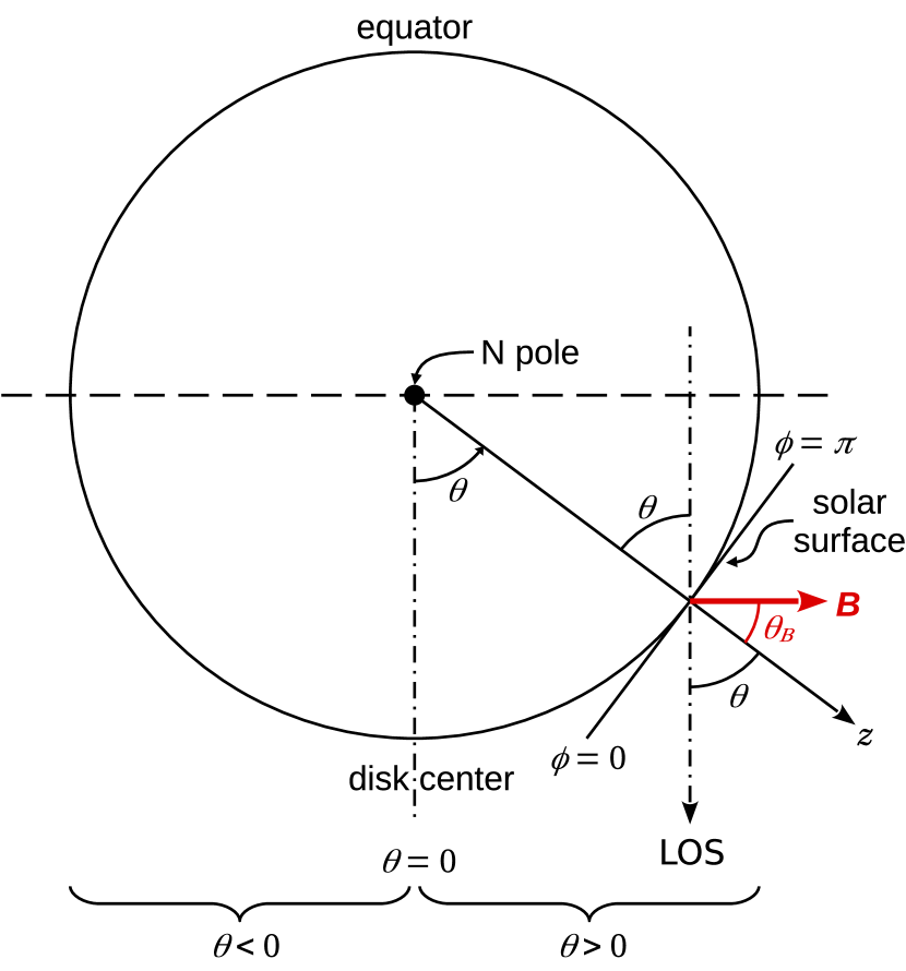
Figure 6: Observing geometry for uniform field computations with HanleRT used in the panels of Figure 7. Note the convention for negative LOS $\theta$.

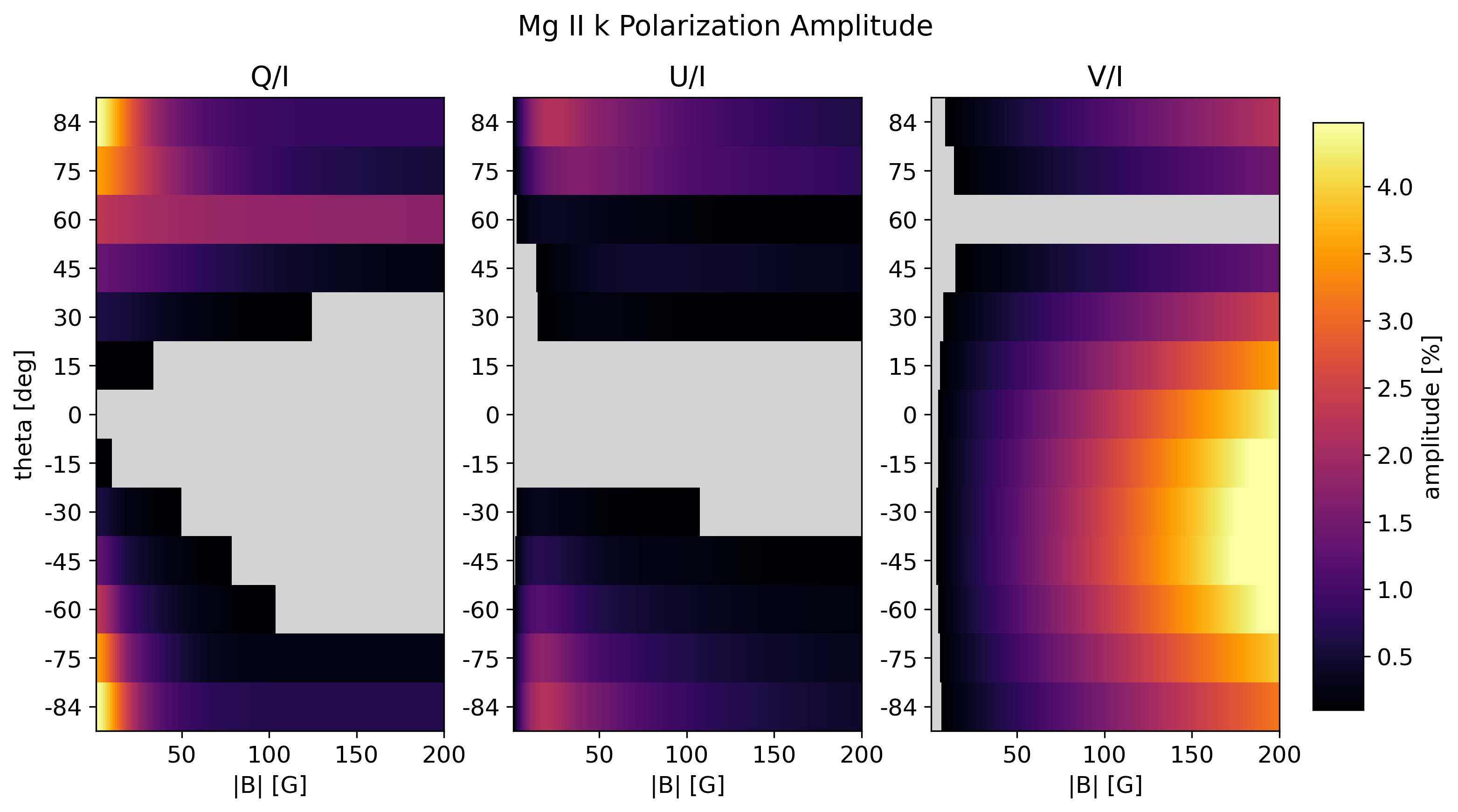
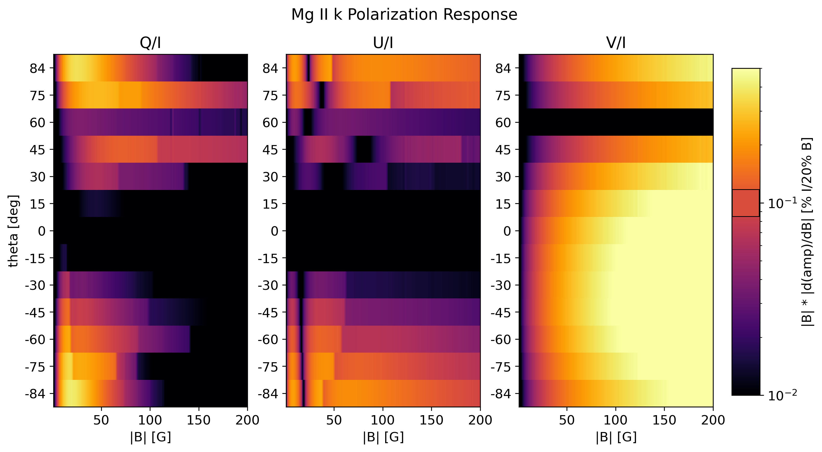
Figure 7: Top: “Heat Map” of the Mg II k core polarization amplitude for a uniform magnetic field inclined at $\theta_{B}=-30^{\circ}$ from vertical. Gray regions are where the amplitude falls below 0.1% of the intensity, here taken as a typical instrumental SNR. Bottom: Derivative of polarization amplitude data from the top panel with respect to magnetic field to produce a “heat map” of the response. The color scale gives the relative change in amplitude of the spectral feature in response to a 20% change in $|B|$. Regions of the map brighter than the 0.1% value on the color scale (highlighted by black box) indicate an observing geometry that could infer $|B|$ to within 20% assuming an instrumental polarization SNR of 0.1% of the intensity. See text for further details.

In Figures 1 and 2 we saw how the Mg II $k$ line has contributions from plasma that is highest in the Sun’s atmosphere. The $h$ line is a factor of two less opaque, but it has a higher Landé g-factor than $k$ and so is more sensitive to the Zeeman effect (Ishikawa et al., 2021). However, its upper $J=1/2$ level is unpolarizable and so it can have no Hanle effect in the line core.

Both the Zeeman and Hanle effects can and should be used to probe chromospheric magnetism. The Zeeman effect produces the largest polarimetric signals when fields are relatively strong (average flux densities of a few hundred Mx cm^-2 were measured using the weak field limit applied to the Mg lines by Ishikawa et al., 2021). However, for weaker fields, the Hanle effect becomes the dominant source of polarized light variations in response to the solar magnetic fields. Following early theoretical work by Belluzzi & Trujillo Bueno (2012), the scattering polarization, Hanle and Zeeman effects across the $h$ and $k$ lines was investigated in semi-empirical 1D models (Alsina Ballester et al., 2016; del Pino Alemán et al., 2016, 2020). The Hanle field of the $k$ line is 23 G (see Figure 5). These authors demonstrated that, for field strengths of the order of 10 G, measurable variations of the order of $\sim$1% in the fractional linear polarization of Mg II $k$ are produced by the Hanle effect. Here, we extend this work with a larger grid of LOS angles and magnetic field strengths (see Figure 6 for the geometry) and show polarization amplitude and magnetic response “heat maps” in Figure 7. As in del Pino Alemán et al. (2020) we used HanleRT to compute the intensity and polarization from a Mg II 3-term atom including PRD effects in atmosphere C of Fontenla et al. (1993). We computed profiles for a grid of uniform magnetic field vectors inclined at $\theta_{B}=-30^{\circ}$ from vertical, with fixed azimuth, and with $|B|$ ranging from 1 to 200 G at 1 G intervals. These values of $|B|$ are about 20 and 10 times smaller and larger, respectively, than the Hanle field. We computed the emergent Stokes profiles for 13 LOS viewing angles $\theta$ ranging from $+75^{\circ}{}$ to $-75^{\circ}{}$ at 15^∘ intervals, as well as $\mu=\cos(\theta)=0.1$, which corresponds to $\theta\sim\pm 84.5$^∘ or a limb distance of about 5^′′. We examine the relative variation in the amplitude of the fractional polarization (hereafter simply “response“), $|B|\cdot dA_{i}/dB$, where $i$ indicates the polarization $Q$, $U$, or $V$, and $A_{i}$ is the amplitude, $A_{i}=({\rm max}(i)-{\rm min}(i))/I\cdot 100\%$, within the Mg II k core region. The top panel of 7 shows the amplitude $A_{i}$, while the bottom panel shows the response with respect to magnetic field over the full range of $|B|$ and LOS $\theta$. The units of the response are $\%I/\%B$, and we have scaled the data such that the denominator represents a 20% change in $|B|$. Under this normalization, a response of 1 corresponds to a 1% amplitude change for a 20% change in $|B|$.

In order to assess the practical application of these calculations, we consider noise at the level of $\sim 0.1\%$ of intensity ($10^{-3}I$). Those regions in the response heat map brighter than that value on the color scale are where the instrument would be able to infer components of the magnetic field to within 20%. We conclude that we would be able to reasonably estimate this vector orientation for magnetic field strengths of $\sim$5 to 50 G at observation angles from about $\theta=\pm 45^{\circ}$ to the limb due to the Hanle effect in $Q$ and/or $U$, and stronger line-of-sight fields at nearly any observation angle from the Zeeman effect in Stokes $V$. The largest sensitivity in $Q$ and $U$ occurs for observations near the limb and field strengths below the critical Hanle field. (Dark vertical strips in the response of Stokes $U$ are due to local maxima in the amplitude curve near the critical Hanle field for Mg II $k$; compare to the top panel of Figure 7). The $V$ amplitude is constant and zero at $\theta=60^{\circ}$ as this is the angle where the magnetic field vector is orthogonal to the line-of-sight. Measurable linear polarization is produced at that geometry, however its variation with magnetic field is too low to be used as a diagnostic. “Heat map” diagrams for other field inclination angles are qualitatively similar, with the regions of maximum response due to the Hanle and Zeeman effects shifting in relation to the field & LOS geometry.

We conclude that diagnosing magnetic field from the Hanle effect in Mg II $k$ is feasible for a large range of geometries and with achievable signal-to-noise ratios. The range of field strengths to which the Hanle effect is sensitive complement those higher field strengths ($|B|\geq 50$G) to which the Zeeman effect is sensitive, for the case of the Mg II $k$ line.

Additional work on the Hanle effect in the lines of Fe II is underway and will be reported elsewhere. Importantly, there is at least one line (at 2744.01 Å) with a Hanle field above 60 G, and several where the critical field exceeds that of the Mg II $k$ line.

2.6 Addressing the “corrugation problem”

Figure 2 shows how state-of-the-art numerical models lead to contours in optical depth which can be far from horizontal. The free energy in these MHD simulations generated by convection and emerging flux leads to highly dynamic evolution in the lower density regions of most interest to us at the top of the chromosphere. The geometric distortions of the $\tau=1$ surfaces in these tenuous regions naturally reflect the low inertia of the plasma, subjected to Lorentz, pressure gradient and gravitational forces, evolving in response to the forcing from below. But, as noted earlier, the extreme corrugations of order 10 Mm are not negligible compared with the scale of the emerging flux system itself. The question then arises, how can we infer magnetic field at a constant geometric height, if we are to apply mathematical techniques to estimate the free energy and topology within the corona? Progress can be anticipated without such techniques, by direct comparison of numerical prediction and measurements. But this question must be addressed if we are to measure the development of free energy in the overlying corona in time, in general.

Let us assume that the calculations are a reasonable, “first order” approximation to the kind of geometric distortions of the $\tau=1$ surfaces of sets of lines. The advantage of observing the 259-281 nm region is that we know the order of the opacities of each line in a sequence: the Mg II lines are the most opaque, next come the sextet system transitions of Fe II and then the quartet systems, each with its spread of oscillator strengths. Thus, given a calculation, we can (as in Figure 2) find the $\tau=1$ surfaces. We could compute Stokes profiles and associate a magnetic field from such synthetic data, knowing the heights of each line’s formation.

But this is not the situation we face with the remotely-sensed Stokes data, we have no knowledge other than the Stokes profiles of many lines, on a two dimensional geometric image of the Sun at each wavelength. Fortunately, this problem fits well into the picture of machine learning algorithms (e.g. Bobra & Mason, 2021). Synthetic data can be used to train an algorithm to find level geometric surfaces (Asensio Ramos & Díaz Baso, 2019) of direct use for mathematics to derive quantities of interest. The large coverage of optical depths of the 256-281 nm region and the variety of Hanle field strengths strongly suggest that, if the models are sufficiently complete to represent the atmospheric dynamics and temperature structure, then such an algorithm should have a non-zero probability of yielding the desired results. The combined use of Hanle and Zeeman effects enhances this probability, at least in principle. We are exploring ways in which this program of research might be implemented.

3 Discussion

In this paper we have examined the general problem of identifying the sources of magnetic energy within coronal plasma, which leads to flaring, plasmoid and CME ejections. By a process of elimination, we arrived at a wavelength range between 2560 and 2810 Å, which appears to be the most promising range in which to measure conditions at the coronal base. Our conclusions build upon the important study of Trujillo Bueno et al. (2017), not only by seeking answers to questions concerning the magnetic free energy and topology, aimed at understanding the origins of phenomena responsible for Space Weather. Our conclusions also differ by proposing a potentially ideal, relatively narrow spectral region between 256 and 281 nm, expanding significantly the 279.2-280.7 region selected by the CLASP2 mission, to serve as a basis for future, more targeted research.

To achieve measurements in this region clearly will require a space-based platform for spectropolarimetry. These conclusions are based upon several criteria: The spectrum must be bright enough; spectral features must extend as high as possible; the spectral features must contain information on magnetic fields through both the Zeeman and Hanle effects; the spectra must be demonstrably unblended; lines with multiple opacities are needed to span across the corrugated surfaces that are present at the coronal base.

Thus we suggest that a novel spectropolarimeter, building upon a heritage from SKYLAB, SMM (UVSP), SoHO (SUMER), IRIS, CLASP and CLASP2, be considered for flight to address the problems of interest to science and society. Such a mission would complement the unique capabilties of the Daniel K. Inouye Solar Telescope which can observe important chromospheric lines (include all those shown in the top row of Figure 1) from the ground, at a sub-arcsecond spatial resolution and/or high cadence.

Finally, it is important to note that the CLASP2 measurements of Ishikawa et al. (2021) achieved signal-to-noise ratios of over 1000 in the Mg II line cores. This demonstrates that a modest, D=25 cm telescope operating at NUV wavelengths is sufficient for delivering the weak signals required for diagnosis of magnetic fields, over active regions at least, where the magnetic flux density exceeds 100 Mx cm^-2.

Line blends and missing opacity

The NUV region is well-known as a crowded region of the solar spectrum, and also a region where some opacity appears to be “missing”. The effects of this missing opacity are examined below using comparisons of detailed simulations and observations. It can be significant at certain wavelengths, but does it not affect the cores of strong chromospheric lines. (See also discussions by Fontenla et al., 2011; Peterson et al., 2017). Line blending is however a concern.

We have addressed blending using data from the Hubble Space Telescope, from the SO82B spectrograph on SKYLAB, and using sophisticated radiative transfer models. The models are based on Local Thermodynamic Equilibrium (LTE) radiative transfer models computed using TURBOSPECTRUM (Plez, 2012), and adopting a custom calculated Solar 1D, spherical MARCS model atmosphere (Gustafsson et al., 2008). A complete linelist in the corresponding spectral region was adopted in the computations from the VALD database (Ryabchikova et al., 2011). The linelist includes up-to-date atomic data, including line-broadening parameters from collisions with neutral hydrogen atoms, calculated ab-initio following Barklem et al. (1998) for all neutral atoms including dominant Mg II lines and iron group elements.

A comparison of high resolution Hubble spectra of $\alpha$ Cen A with the models is informative. A typical example in an interesting region of the NUV spectrum is shown in Figure 8. The blue line represents the flux spectrum computed for the Sun, the red line the spectrum of $\alpha$ Cen A. The flux densities shown are computed at the respective stellar surfaces, with no ad-hoc adjustments of either scale.

Figure 8: Flux spectra computed for a Solar atmospheric model (blue) using 1D, LTE radiative transfer calculations (see Section Line blends and missing opacity) are shown along with spectra of the Sun-like star $\alpha$ Cen A (red) obtained with the STIS instrument on the HST. The data are a composite of several exposures from the E230H grating, assembled and processed by Ayres (2014). The STIS data were shifted according to the redshift of 22.4 km s^-1, and converted to flux at the stellar surface using the angular diameter of 9.09 milli-arcsec. The spectra are compared with no adjustment of flux or wavelength scale. The qualitative agreement is remarkable. The units are Å (wavelength) and erg cm^-2 s^-1 Å^-1 (flux, $F=\pi\overline{I}$, where $\overline{I}$ is the mean disk intensity).

The comparison is remarkable, particularly in the cores of some of the strong lines, most of which belong to Fe II. Wavelengths are evident (near 2623 Å for example) where opacity appears to be missing (blue line above red line), but in the Fe II lines identified in the figure there is no evidence for missing opacity, if anything, the observed line cores in red lie above the blue line, indicating emission from the star’s chromosphere.

The model calculations also permit us to identify possible blends (Figure 9). This figure shows two computations, black is the full model calculation (also shown in blue in Figure 8), and in this figure blue is a calculation using opacity only from the Fe II lines. When significant differences between black and blue lines exist, these are wavelengths where opacities are present in lines other than Fe II. Conversely, when they agree, the Fe II spectrum dominates and these are essentially unblended wavelengths. As noted in the main text, the wavelength region above 281 and below 310 nm does not contain strong lines formed in the middle-high chromosphere, therefore these are not shown here. Above 281 nm the lack of such lines makes this a less desirable region because blending becomes a bigger problem.

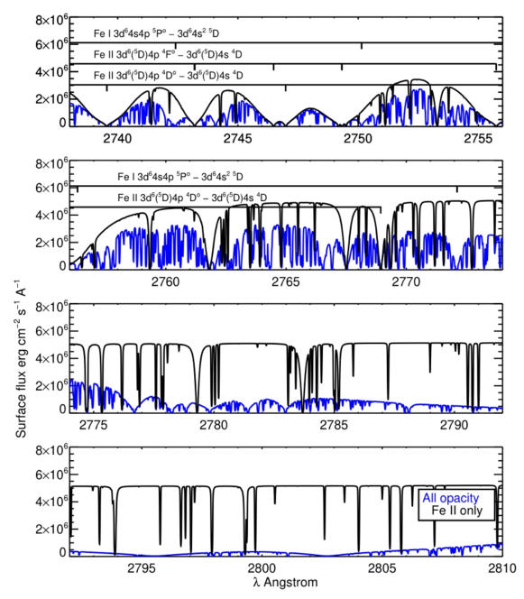
Figure 9: Two calculations are shown for the solar NUV spectrum: one (black) is made with the full set of lines, and the other (red) is made where lines of Fe II are the only sources of opacity. Strong lines from the quartet system of Fe II are annotated, along with lines of Fe I whose opacity is much smaller. The cores of the strong lines of Fe II are dominated by Fe II itself, the region above $\approx$ 265 nm is, aside from narrow lines, dominated by wings of the Mg II $h$ and $k$ lines.

Lastly we can, to some extent, check for blends independently of the model computations. Rutten & Stencel (1980) were able to find weak lines in the wings of the Ca II $H$ and $K$ lines looking to data obtained near the solar limb. In Figure 10 we show (with an arbitrary flux calibration), spectra of $\alpha$ Cen A with spectra from the SO82B spectrograph on SKYLAB. The latter are taken from the scans across a quiet region of solar limb obtained on August 27 1973, the slit being tangential to the limb and stepped by 2” between pointings. These are the photographic data analyzed by Doschek et al. (1977). The “intensities” plotted here are photographic densities. But these densities suffice for us to find significant blends, which will potentially be revealed by changes in the spectra as the spectrograph slit was repointed from 2” inside the limb to 6” outside, in 2” steps.

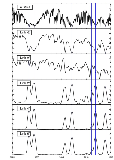
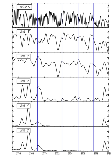
Figure 10: The left panel shows the spectral region close to the sextet resonance lines of Fe II is shown from $\alpha$ Cen A (top), and 5 spectra representative of the spectra as a function of position relative to the solar limb. The right panel shows the 2765-2780 Å region. Blue lines mark wavelengths of Fe II transitions. The three other lines seen in emission in the right panel are from Cr II at 2766.52 Å, and questionable identifications of Fe II 2767.50, a transition between high lying states, and of Mg I at 2779.8 Å (Doschek et al., 1977).

Different behaviors are seen depending on the line of interest. In the wavelength range from 2595 to 2615 Å (left panel, showing resonance lines of the sextet system) there is no evidence of blended features. But the right panel of Figure 10 shows a spectral region containing lines of the quartet system of Fe II. In contrast to the resonance sextet transitions, here we find that essentially no Fe II lines are strong enough to be unblended. However, a plot of similar transitions (not shown) between 2750 and 2765 Å has stronger lines at 2756 and 2762 Å which are not strongly blended. These conclusions have been verified using NRL report 8653 (Moore et al., 1982), from which the last column of Table 1 has been constructed. There are only four lines which are classified as severely blended of all the quartets, sextets of Fe II and quintets of Fe I.

References

- Allen (1973) Allen, C. W. 1973, Astrophysical quantities (Athlone Press, Univ. London)
- Alsina Ballester et al. (2016) Alsina Ballester, E., Belluzzi, L., & Trujillo Bueno, J. 2016, ApJL, 831, L15, doi: 10.3847/2041-8205/831/2/L15
- Asensio Ramos & Díaz Baso (2019) Asensio Ramos, A., & Díaz Baso, C. J. 2019, A&A, 626, A102, doi: 10.1051/0004-6361/201935628
- Athay & Dere (1991) Athay, R. G., & Dere, K. P. 1991, ApJ, 379, 776, doi: 10.1086/170553
- Auer et al. (1980) Auer, L. H., Rees, D. E., & Stenflo, J. O. 1980, A&A, 88, 302
- Ayres (2014) Ayres, T. R. 2014, in Astronomical Society of India Conference Series, Vol. 11, Astronomical Society of India Conference Series, 1
- Barklem et al. (1998) Barklem, P. S., Anstee, S. D., & O’Mara, B. J. 1998, PASA, 15, 336, doi: 10.1071/AS98336
- Barnes et al. (2016) Barnes, G., Leka, K. D., Schrijver, C. J., et al. 2016, ApJ, 829, 89, doi: 10.3847/0004-637X/829/2/89
- Belluzzi & Trujillo Bueno (2012) Belluzzi, L., & Trujillo Bueno, J. 2012, ApJL, 750, L11, doi: 10.1088/2041-8205/750/1/L11
- Berdyugina & Fluri (2004) Berdyugina, S. V., & Fluri, D. M. 2004, A&A, 417, 775, doi: 10.1051/0004-6361:20034452
- Berdyugina & Solanki (2002) Berdyugina, S. V., & Solanki, S. K. 2002, A&A, 385, 701, doi: 10.1051/0004-6361:20020130
- Berdyugina et al. (2003) Berdyugina, S. V., Solanki, S. K., & Frutiger, C. 2003, A&A, 412, 513, doi: 10.1051/0004-6361:20031473
- Bird (1982) Bird, M. K. 1982, Space Sci. Rev., 33, 99, doi: 10.1007/BF00213250
- Bird & Edenhofer (1990) Bird, M. K., & Edenhofer, P. 1990, Physics and Chemistry in Space, Vol. 20, Physics of the Inner Heliosphere I. Large-Scale Phenomena. (Berlin Heidelberg: Springer-Verlag), 13–97
- Bobra & Mason (2021) Bobra, M., & Mason, J. 2021, ”Machine Learning, Statistics, and Data Mining for Heliophysics”, doi: https://doi.org/10.5281/zenodo.1412824.
- Bobra & Couvidat (2015) Bobra, M. G., & Couvidat, S. 2015, The Astrophysical Journal, 798, 135, doi: 10.1088/0004-637x/798/2/135
- Carmichael (1964) Carmichael, H. 1964, NASA Special Publication, 50, 451
- Casini et al. (2017) Casini, R., White, S. M., & Judge, P. G. 2017, SSR, 210, 145
- Cauzzi et al. (2008) Cauzzi, G., Reardon, K. P., Uitenbroek, H., et al. 2008, A&A, 480, 515, doi: 10.1051/0004-6361:20078642
- Centeno et al. (2010) Centeno, R., Trujillo Bueno, J., & Asensio Ramos, A. 2010, ApJ, 708, 1579, doi: 10.1088/0004-637X/708/2/1579
- Chandrasekhar (1961) Chandrasekhar, S. 1961, Hydrodynamic and hydromagnetic stability
- Chen et al. (2019) Chen, Y., Manchester, W. B., Hero, A. O., et al. 2019, Space Weather, 17, 1404, doi: 10.1029/2019SW002214
- De Pontieu et al. (2020) De Pontieu, B., Martínez-Sykora, J., Testa, P., et al. 2020, ApJ, 888, 3, doi: 10.3847/1538-4357/ab5b03
- del Pino Alemán et al. (2016) del Pino Alemán, T., Casini, R., & Manso Sainz, R. 2016, ApJL, 830, L24
- del Pino Alemán et al. (2020) del Pino Alemán, T., Trujillo Bueno, J., Casini, R., & Manso Sainz, R. 2020, ApJ, 891, 91
- Deshmukh et al. (2020) Deshmukh, V., Berger, T., Meiss, J., & Bradley, E. 2020, arXiv e-prints, arXiv:2012.14405
- Díaz Baso et al. (2019) Díaz Baso, C. J., Martínez González, M. J., & Asensio Ramos, A. 2019, A&A, 625, A128, doi: 10.1051/0004-6361/201834790
- Doschek et al. (1977) Doschek, G. A., Feldman, U., & Cohen, L. 1977, ApJS, 33, 101, doi: 10.1086/190421
- Eddy (2009) Eddy, J. A. 2009, The Sun, the Earth and Near-Earth Space: A Guide to the Sun-Earth System (NASA)
- Fleishman et al. (2017) Fleishman, G. D., Anfinogentov, S., Loukitcheva, M., Mysh’yakov, I., & Stupishin, A. 2017, ApJ, 839, 30, doi: 10.3847/1538-4357/aa6840
- Fontenla et al. (1993) Fontenla, J. M., Avrett, E. H., & Loeser, R. 1993, ApJ, 406, 319
- Fontenla et al. (2011) Fontenla, J. M., Harder, J., Livingston, W., Snow, M., & Woods, T. 2011, Journal of Geophysical Research (Atmospheres), 116, D20108, doi: 10.1029/2011JD016032
- Fox et al. (2016) Fox, N. J., Velli, M. C., Bale, S. D., et al. 2016, Space. Sci. Rev., 204, 7, doi: 10.1007/s11214-015-0211-6
- Gandorfer (2000) Gandorfer, A. 2000, The Second Solar Spectrum: A high spectral resolution polarimetric survey of scattering polarization at the solar limb in graphical representation. Volume I: 4625 Å to 6995 Å
- Gelfreikh (1994) Gelfreikh, G. B. 1994, in IAU Colloq. 144, Solar Coronal Structures, ed. V. Rusin, P. Heinzel, & J.-C. Vial (Bratislava, Slovakia: VEDA Publishing Company), 21–28
- Gold & Hoyle (1960) Gold, T., & Hoyle, F. 1960, MNRAS, 120, 89
- Gudiksen et al. (2011) Gudiksen, B. V., Carlsson, M., Hansteen, V. H., et al. 2011, A&A, 531, A154
- Gustafsson et al. (2008) Gustafsson, B., Edvardsson, B., Eriksson, K., et al. 2008, A&A, 486, 951, doi: 10.1051/0004-6361:200809724
- Hansteen et al. (2014) Hansteen, V., De Pontieu, B., Carlsson, M., et al. 2014, Science, 346, 1255757, doi: 10.1126/science.1255757
- Hirayama (1974) Hirayama, T. 1974, SoPh, 34, 323
- Ishikawa et al. (2021) Ishikawa, R., Bueno, J. T., del Pino Alemán, T., et al. 2021, Science Advances, 7, doi: 10.1126/sciadv.abe8406
- Jonas et al. (2018) Jonas, E., Bobra, M. G., Shankar, V., Hoeksema, J. T., & Recht, B. 2018, Solar Physics, 293, 1
- Judge et al. (2001) Judge, P., Casini, R., Tomczyk, S., Edwards, D. P., & Francis, E. 2001, Coronal Magnetogmetry: a feasibility study, Tech. Rep. NCAR/TN-446-STR, National Center for Atmospheric Research
- Judge (2020) Judge, P. G. 2020, The Sun: A Very Short Introduction (Oxford University Press)
- Judge (2021) Judge, P. G. 2021, ApJ, in press
- Judge et al. (2013) Judge, P. G., Habbal, S., & Landi, E. 2013, SoPh, 288, 467
- Judge et al. (2012) Judge, P. G., Kleint, L., Casini, R., & Schad, T. 2012, in American Astronomical Society Meeting Abstracts, Vol. 220, American Astronomical Society Meeting Abstracts #220, 521.19
- Judge et al. (2014) Judge, P. G., Kleint, L., Donea, A., Sainz Dalda, A., & Fletcher, L. 2014, ApJ, 796, 85
- Judge et al. (2015) Judge, P. G., Kleint, L., & Sainz Dalda, A. 2015, ApJ, 814, 100, doi: 10.1088/0004-637X/814/2/100
- Judge et al. (2011) Judge, P. G., Tritschler, A., & Low, B. C. 2011, ApJL, 730, L4, doi: 10.1088/2041-8205/730/1/L4
- Kano et al. (2017) Kano, R., Trujillo Bueno, J., Winebarger, A., et al. 2017, ApJL, 839, L10, doi: 10.3847/2041-8213/aa697f
- Kleint & Gandorfer (2017) Kleint, L., & Gandorfer, A. 2017, Space Science Reviews, 210, 397, doi: 10.1007/s11214-015-0208-1
- Kopp & Pneuman (1976) Kopp, R., & Pneuman, G. 1976, SoPh, 50, 85
- Korsós et al. (2020) Korsós, M. B., Georgoulis, M. K., Gyenge, N., et al. 2020, ApJ, 896, 119, doi: 10.3847/1538-4357/ab8fa2
- Kramar et al. (2006) Kramar, M., Inhester, B., & Solanki, S. K. 2006, A&A, 456, 665, doi: 10.1051/0004-6361:20064865
- Kuckein et al. (2012) Kuckein, C., Martínez Pillet, V., & Centeno, R. 2012, A&A, 539, A131
- Landi Degl’Innocenti (2007) Landi Degl’Innocenti, E. 2007, A&A, 461, 1, doi: 10.1051/0004-6361:20042232
- Landi degl’Innocenti & Landolfi (2004) Landi degl’Innocenti, E. L., & Landolfi, M. 2004, Astrophysics and Space Library, Vol. 307, Polarization in Spectral Lines (Dordrecht: Kluwer Academic Publishers)
- Leka et al. (2019) Leka, K. D., Park, S.-H., Kusano, K., et al. 2019, ApJs, 243, 36, doi: 10.3847/1538-4365/ab2e12
- Li et al. (2017) Li, W., Jönsson, P., Brage, T., & Hutton, R. 2017, Phys. Rev. A., 96, 052508, doi: 10.1103/PhysRevA.96.052508
- Li et al. (2020) Li, X., Zheng, Y., Wang, X., & Wang, L. 2020, ApJ, 891, 10, doi: 10.3847/1538-4357/ab6d04
- Liu et al. (2019) Liu, H., Liu, C., Wang, J. T. L., & Wang, H. 2019, ApJ, 877, 121, doi: 10.3847/1538-4357/ab1b3c
- Loukitcheva (2014) Loukitcheva, M. 2014, in 40th COSPAR Scientific Assembly, Vol. 40, E2.2–28–14
- Loukitcheva (2020) Loukitcheva, M. 2020, Frontiers in Astronomy and Space Sciences, 7, 45, doi: 10.3389/fspas.2020.00045
- Low (1994) Low, B. C. 1994, Physics of Plasmas, 1, 1684, doi: 10.1063/1.870671
- Moore et al. (1982) Moore, C. E., Tousey, R., & Brown, C. M. 1982, The solar spectrum 3069 A - 2095 A. From the Echelle Spectrograph flown in 1961 and 1964 (Naval Research Laboratory)
- Nishizuka et al. (2018) Nishizuka, N., Sugiura, K., Kubo, Y., Den, M., & Ishii, M. 2018, ApJ, 858, 113, doi: 10.3847/1538-4357/aab9a7
- Panos & Kleint (2020) Panos, B., & Kleint, L. 2020, ApJ, 891, 17, doi: 10.3847/1538-4357/ab700b
- Park et al. (2018) Park, E., Moon, Y.-J., Shin, S., et al. 2018, ApJ, 869, 91, doi: 10.3847/1538-4357/aaed40
- Peterson et al. (2017) Peterson, R. C., Kurucz, R. L., & Ayres, T. R. 2017, ApJs, 229, 23, doi: 10.3847/1538-4365/aa6253
- Plez (2012) Plez, B. 2012, Turbospectrum: Code for spectral synthesis. http://ascl.net/1205.004
- Rempel (2017) Rempel, M. 2017, ApJ, 834, 10, doi: 10.3847/1538-4357/834/1/10
- Robustini et al. (2018) Robustini, C., Leenaarts, J., & de la Cruz Rodríguez, J. 2018, A&A, 609, A14, doi: 10.1051/0004-6361/201731504
- Rutten & Stencel (1980) Rutten, R. J., & Stencel, R. E. 1980, A&AS, 39, 415
- Ryabchikova et al. (2011) Ryabchikova, T. A., Pakhomov, Y. V., & Piskunov, N. E. 2011, Kazan Izdatel Kazanskogo Universiteta, 153, 61
- Schad et al. (2016) Schad, T. A., Penn, M. J., Lin, H., & Judge, P. G. 2016, ApJ, 833, 5, doi: 10.3847/0004-637X/833/1/5
- Solanki et al. (2003) Solanki, S. K., Lagg, A., Woch, J., Krupp, N., & Collados, M. 2003, Nature, 425, 692, doi: 10.1038/nature02035
- Sturrock (1966) Sturrock, P. A. 1966, Nature, 211, 695
- Trujillo Bueno & Asensio Ramos (2007) Trujillo Bueno, J., & Asensio Ramos, A. 2007, ApJ, 655, 642, doi: 10.1086/509795
- Trujillo Bueno et al. (2017) Trujillo Bueno, J., Landi Degl’Innocenti, E., & Belluzzi, L. 2017, Space Science Reviews, 210, 183, doi: 10.1007/s11214-016-0306-8
- Trujillo Bueno et al. (2018) Trujillo Bueno, J., Štěpán, J., Belluzzi, L., et al. 2018, ApJL, 866, L15, doi: 10.3847/2041-8213/aae25a
- Uitenbroek (2001) Uitenbroek, H. 2001, ApJ, 557, 389
- Uitenbroek (2010) —. 2010, Mem. Soc. Astron. Italia, 81, 701
- Viotti et al. (1988) Viotti, R., Vittone, A., & Friedjung, M. 1988, Physics of formation of FE II lines outside LTE, Vol. 138, doi: 10.1007/978-94-009-4023-9
- Štěpán & Trujillo Bueno (2010) Štěpán, J., & Trujillo Bueno, J. 2010, ApJL, 711, L133, doi: 10.1088/2041-8205/711/2/L133
- Wang et al. (2016) Wang, Y., Su, Y., Hong, Z., et al. 2016, ApJ, 833, 250, doi: 10.3847/1538-4357/833/2/250
- White (2004) White, S. M. 2004, Coronal Magnetic Field Measurements Through Gyroresonance Emission, ed. D. E. Gary & C. U. Keller, Vol. 314, 89, doi: 10.1007/1-4020-2814-8_5
- Wiegelmann & Sakurai (2021) Wiegelmann, T., & Sakurai, T. 2021, Living Reviews in Solar Physics, 18, 1, doi: 10.1007/s41116-020-00027-4