Stability and bifurcation of mixing in the Kuramoto model with inertia

Abstract

The Kuramoto model of coupled second order damped oscillators on convergent sequences of graphs is analyzed in this work. The oscillators in this model have random intrinsic frequencies and interact with each other via nonlinear coupling. The connectivity of the coupled system is assigned by a graph which may be random as well. In the thermodynamic limit the behavior of the system is captured by the Vlasov equation, a hyperbolic partial differential equation for the probability distribution of the oscillators in the phase space. We study stability of mixing, a steady state solution of the Vlasov equation, corresponding to the uniform distribution of phases. Specifically, we identify a critical value of the strength of coupling, at which the system undergoes a pitchfork bifurcation. It corresponds to the loss of stability of mixing and marks the onset of synchronization. As for the classical Kuramoto model, the presence of the continuous spectrum on the imaginary axis poses the main difficulty for the stability analysis. To overcome this problem, we use the methods from the generalized spectral theory developed for the original Kuramoto model. The analytical results are illustrated with numerical bifurcation diagrams computed for the Kuramoto model on Erdős–Rényi and small-world graphs.

Applications of the second-order Kuramoto model include power networks, coupled pendula, and various biological networks. The analysis in this paper provides a mathematical description of the onset of synchronization in these systems.

1 Introduction

In this paper, we study the following system of coupled second order damped oscillators on a convergent sequence of graphs $\{\Gamma_{n}\}$:

$$\ddot{\theta}_{i}+\gamma\dot{\theta}_{i}=\omega_{i}+\frac{2K}{n}\sum^{n}_{j=1}a^{n}_{ij}\sin\left(\theta_{j}-\theta_{i}\right),\quad i\in[n]=\{1,2,\dots,n\},$$ (1.1)

where $\theta_{i},i\in[n],$ denotes the phase of the $i$th oscillator, $\gamma>0$ is a damping constant, $K$ is the coupling strength and $a^{n}_{ij}$ is the adjacency matrix of $\Gamma_{n}$. Intrinsic frequencies $\omega_{i},i\in[n],$ are independent identically distributed random variables drawn from the probability distribution with density $g$. By rescaling time, intrinsic frequencies, and $K$, one can make $\gamma=1$, which will be assumed without loss of generality throughout this paper.

System of ordinary differential equations (1.1) may be viewed as an extension of the classical Kuramoto model (KM), which is used to study collective behavior in large coupled systems [8]. In this context, it is called the KM with inertia, because the second order terms in (1.1) introduce inertial effects into the system’s dynamics. On the other hand, system (1.1) has a clear mechanical interpretation. For instance, it may be viewed as a system of coupled pendula or coupled power generators, as it is perhaps best known for [11, 15]. Like its classical counterpart, the KM with inertia features transition to synchronization. For small positive values of the coupling strength, the system exhibits irregular dynamics, called mixing. Upon increasing the coupling strength $K$, mixing loses stability and a gradual (soft) transition to synchronization takes place. The onset of synchronization in the classical KM with all-to–all coupling was analyzed in [1, 5] and in the model on graphs in [3, 4]. The analysis of synchronization in the KM with inertia involves new technical challenges related to the dimensionality of the phase space, which make it an interesting stability problem. In addition, synchronization in the KM with inertia has important applications. First, synchronization provides a more efficient regime of operation of power networks. Therefore, it is important to know what factors determine stability of synchrony in the second order model on graphs. Previous studies of the onset of synchronization in the KM with inertia [14, 13] relied on asymptotic analysis and numerical simulations. In this work, for the first time we perform a rigorous linear stability analysis of mixing and identify the instability of mixing. Furthermore, we perform a formal center manifold reduction and identify the bifurcation, marking the onset of synchronization, as a pitchfork bifurcation. We verified these results numerically for the KM on various graphs including Erdős-Rényi (ER) and small-world (SW) graphs.

To proceed, we rewrite (1.1) as a system of coupled second order ordinary differential equations and add a separate equation for $\omega_{i}$:

$$\begin{split}\dot{\theta}_{i}&=\psi_{i}+\omega_{i},\\ \dot{\psi}_{i}&=-\psi_{i}+\frac{2K}{n}\sum^{n}_{j=1}a^{n}_{ij}\sin(\theta_{j}-\theta_{i}),\\ \dot{\omega}_{i}&=0,\qquad i\in[n].\end{split}$$ (1.2)

To study the dynamics of (1.2) for large $n$, we employ the following Vlasov equation

$$\partial_{t}f+\partial_{\theta}\left((\psi+\omega)f\right)+\partial_{\psi}\left((-\psi+\mathbf{N}[f])f\right)=0,\quad f=f(t,\theta,\psi,\omega,x),$$ (1.3)

where

$$\mathbf{N}[f](t,\theta,x)=\frac{K}{{\mathrm{i}\mkern 1.0mu}}\left(e^{-{\mathrm{i}\mkern 1.0mu}\theta}h(t,x)-e^{{\mathrm{i}\mkern 1.0mu}\theta}\overline{h(t,x)}\right).$$

Here and below, we use ${\mathrm{i}\mkern 1.0mu}=\sqrt{-1}$ to denote the imaginary unit. Further, $f(t,\theta,\psi,\omega,x)d\theta d\psi d\omega$ is the probability that the state of the oscillator at point $x\in[0,1]$ at time $t\in\mathbb{R}^{+}$ is in $(\theta,\theta+d\theta)\times(\psi,\psi+d\psi)\times(\omega,\omega+d\omega)$. The justification of the Vlasov equation as a mean field limit for the original KM on graphs can be found in [7, 3]. It extends verbatim to cover the model at hand.

The following local order parameter plays a key role in the analysis of synchronization in the KM model:

$$h(t,x)=\int_{\mathbb{T}\times\mathbb{R}^{2}\times I}W(x,y)e^{{\mathrm{i}\mkern 1.0mu}\theta}f(t,\theta,\psi,\omega,y)d\theta d\psi d\omega dy,$$ (1.4)

where $I=[0,1]$ and $\mathbb{T}=\mathbb{R}/2\pi\mathbb{Z}$. $W$ is a square integrable function on $I^{2}$, which describes the limit of the graph sequence $\{\Gamma_{n}\}$. $W$ is called a graphon. For the details on graph limits and their applications to the continuum description of the dynamical networks, we refer the interested reader to [3, 10].

A weak (distribution–valued) solution $f(t,\theta,\psi,\omega,x)$ of the initial value problem for the Vlasov equation (1.3) yields the probability distribution of particles in the phase space $\mathbb{T}\times\mathbb{R}^{2}$ for each $(t,x)\in\mathbb{R}^{+}\times I$ (cf. [6, 7]). By mixing we call the following steady state solution of (1.3)

$$f_{mix}=\frac{g(\omega)}{2\pi}\delta(\psi),$$ (1.5)

where $\delta$ stands for Dirac’s delta function and $g(\omega)$ is the probability density function characterizing the distribution of intrinsic frequencies. $f_{mix}$ corresponds to the stationary regime when the values of $\theta_{i}$ are distributed uniformly over $\mathbb{T}$. Stability of mixing is the main theme of this paper.

In the next section, we recast the stability problem in the Fourier space and derive the linearized problem. The next step is to characterize the spectrum of the linearized operator. This is done in Section 3. We start by describing the setting for the spectral problem. To this end, we define function spaces and operators involved in the linear stability problem. After that we derive a transcendental equation for the eigenvalues of the linearized problem. The analysis of the eigenvalue problem shows that the bifurcating eigenvalue fails to cross the imaginary axis filled by the residual spectrum. To overcome this difficulty, following the analysis of the classical KM [1, 4], we use the weak formulation for the eigenvalue problem for the linearized operator based on a carefully selected Gelfand triplet and the analytic continuation of the resolvent operator past the imaginary axis. In this setting the generalized eigenvalues are defined as singular points of the generalized resolvent. The corresponding eigenfunction is used in the center manifold reduction of the system’s dynamics. This concludes a rigorous linear stability analysis of mixing and sets the scene for the bifurcation analysis. In Section 3.5, we prove that mixing is asymptotically stable in the subcritical regime. In Section 4, we show that mixing undergoes a pitchfork bifurcation marking the onset of synchronization. The center manifold reduction is done under the assumption of the existence of the center manifold. However, the formal center manifold reduction alone is a formidable problem, as the analysis in this section shows. The proof of existence of the center manifold requires new additional techniques and is beyond the scope of this paper. The analytical results are illustrated with numerical examples of the bifurcation in the KM on ER and SW graphs in Section 5.

2 The Fourier transform

As a probability density function, $g$ is a nonnegative integrable function such that

$$\int_{\mathbb{R}}g(s)ds=1.$$ (2.1)

Since $\omega$ does not change in time, $f$ satisfies the following constraint

$$g(\omega)=\int_{\mathbb{T}\times\mathbb{R}}\!f(t,\theta,\psi,\omega,x)d\theta d\psi,\quad\forall(t,x)\in\mathbb{R}^{+}\times I.$$ (2.2)

In addition, throughout this paper, we will assume the following.

Assumption 2.1.

Let $g$ be a real analytic function. In addition, let the Fourier transform $\hat{g}(\eta):=\int_{\mathbb{R}}e^{{\mathrm{i}\mkern 1.0mu}\eta\omega}g(\omega)d\omega$ be continuous on $\mathbb{R}$ and

$$\lim_{\eta\to\infty}|\hat{g}(\eta)|e^{a\eta}=0$$ (2.3)

for some $0<a<1$.

Remark 2.2.

By the Paley-Wiener theorem, (2.3) implies that $g(\omega)$ has an analytic continuation to the region $0<\mathrm{Im}(z)<a$.

In preparation for the stability analysis of mixing, we rewrite (1.3) using Fourier variables:

$$u_{j}(t,\zeta,\eta,x)=\int_{\mathbb{R}^{2}\times\mathbb{T}}e^{{\mathrm{i}\mkern 1.0mu}(j\theta+\zeta\psi+\eta\omega)}f(t,\theta,\psi,\omega,x)d\theta d\psi d\omega,\quad j\in\mathbb{Z}.$$ (2.4)

The Vlasov PDE is then rewritten as a system of differential equations for the Fourier coefficients $u_{j},\,j\in\mathbb{Z}$:

$$\begin{split}{\partial}_{t}u_{j}&=-\int e^{{\mathrm{i}\mkern 1.0mu}(j\theta+\zeta\psi+\eta\omega)}\frac{\partial}{\partial\theta}\left\{(\psi+\omega)f\right\}d\theta d\psi d\omega\\ &-\int e^{{\mathrm{i}\mkern 1.0mu}(j\theta+\zeta\psi+\eta\omega)}\frac{\partial}{\partial\psi}\left\{(-\psi+\mathbf{N}[f])f\right\}d\theta d\psi d\omega\\ &={\mathrm{i}\mkern 1.0mu}j\int e^{{\mathrm{i}\mkern 1.0mu}(j\theta+\zeta\psi+\eta\omega)}(\psi+\omega)fd\theta d\psi d\omega\\ &\quad+{\mathrm{i}\mkern 1.0mu}\zeta\int e^{{\mathrm{i}\mkern 1.0mu}(j\theta+\zeta\psi+\eta\omega)}\left(-\psi+\frac{K}{{\mathrm{i}\mkern 1.0mu}}(e^{-{\mathrm{i}\mkern 1.0mu}\theta}h-e^{{\mathrm{i}\mkern 1.0mu}\theta}\overline{h})\right)fd\theta d\psi d\omega\\ &=(j-\zeta)\frac{\partial u_{j}}{\partial\zeta}+j\frac{\partial u_{j}}{\partial\eta}+K\zeta(h(t,x)u_{j-1}-\overline{h(t,x)}u_{j+1}),\;j\in\mathbb{Z},\end{split}$$ (2.5)

where

$$h(t,x)=\int_{I}W(x,y)u_{1}(t,0,0,y)dy.$$ (2.6)

is the local order parameter. In addition, we have the following constraints

$$u_{0}(t,0,0,x) = 1,$$ (2.7)

$$u_{-j}(t,-\zeta,-\eta,x) = \overline{u_{j}(t,\zeta,\omega,x)},\;j\in\mathbb{N}.$$ (2.8)

Here, (2.7) follows from (2.2) and (2.8) follows from the fact that $f$ is real. Thus, it is sufficient to restrict to $j\in\mathbb{N}\bigcup\{0\}$ in (2.5).

By changing from $\zeta$ to $\xi$ given by the following relations:

$$\left\{\begin{array}[]{ll}\zeta-j=-e^{-\xi_{j}},&\zeta-j<0,\\ \zeta-j=e^{-\xi_{j}},&\zeta-j\geq 0,\\ \end{array}\right.$$ (2.9)

and setting

$$v_{j}(t,\xi_{j},\eta,x):=\left\{\begin{array}[]{ll}u_{j}(t,j-e^{-\xi_{j}},\eta,x),&\zeta-j<0,\\[5.69046pt] u_{j}(t,j+e^{-\xi_{j}},\eta,x),&\zeta-j\geq 0,\\ \end{array}\right.$$ (2.10)

we obtain

$$\begin{split}\partial_{t}v_{j}&=\partial_{\xi_{j}}v_{j}+j\partial_{\eta}v_{j}+K(j-e^{-\xi_{j}})\left(h(t,x)v_{j-1}-\overline{h(t,x)}v_{j+1}\right),\\ \displaystyle h(t,x)&=\int_{I}W(x,y)v_{1}(t,0,0,y)dy,\end{split}$$

subject to the constraint $v_{0}(t,\infty,\eta,x)=\hat{g}(\eta)$. For $j\geq 0$, we adopt the first line of (2.9) because in the definition of the local order parameter, we need $u_{1}(t,0,0,x)$, for which $\zeta-j=-1<0$. By the same reason, we use the second line for $j\leq-1$.

The steady state of the Vlasov equation, $f_{mix}$, in the Fourier space has the following form

$$v_{0}=\hat{g}(\eta),\quad v_{j}=0,j\in\mathbb{N}.$$ (2.11)

To investigate the stability of (2.11), let $w_{0}=v_{0}-\hat{g}(\eta)$ and $w_{j}=v_{j}$ for $j\neq 0$. Then we obtain the system

$$\left\{\begin{array}[]{l}\displaystyle\partial_{t}w_{1}=\partial_{\xi_{1}}w_{1}+\partial_{\eta}w_{1}+K(1-e^{-\xi_{1}})\left(h(t,x)\hat{g}(\eta)+h(t,x)w_{0}-\overline{h(t,x)}w_{2}\right),\\[11.38092pt] \displaystyle\frac{dw_{j}}{dt}=\frac{\partial w_{j}}{\partial\xi_{j}}+j\frac{\partial w_{j}}{\partial\eta}+K(j-e^{-\xi_{j}})\left(h(t,x)w_{j-1}-\overline{h(t,x)}w_{j+1}\right),\;j\geq 0\;\mbox{and}\;j\neq 1.\\[11.38092pt] \displaystyle h(t,x)=\int_{I}W(x,y)w_{1}(t,0,0,y)dy,\end{array}\right.$$ (2.12)

and $w_{0}(t,\infty,\eta,x)=0$. Our goal is to investigate the stability and bifurcations of the steady state (mixing) $w_{j}=0,\,j\in\mathbb{Z}$ of this system.

The linearized system has the following form

$$\frac{dw_{1}}{dt} = \boldsymbol{L}_{1}[w_{1}]+K\boldsymbol{B}[w_{1}]=:\boldsymbol{S}[w_{1}]$$ (2.13)

$$\frac{dw_{j}}{dt} = \boldsymbol{L}_{j}[w_{j}],\quad j\geq 0\;\mbox{and}\;j\neq 1,$$ (2.14)

where

$$\boldsymbol{L}_{j}[\phi](\xi,\eta,x) = \left({\partial_{\xi}}+j{\partial_{\eta}}\right)\phi(\xi,\eta,x),\;j\in\mathbb{Z}$$ (2.15)

$$\boldsymbol{B}[\phi](\xi,\eta,x) = (1-e^{-\xi})\hat{g}(\eta)\boldsymbol{W}[\phi(0,0,\cdot)](x),$$ (2.16)

and

$$\boldsymbol{W}[f](x)=\int_{\mathbb{R}}W(x,y)f(y)dy.$$ (2.17)

3 The spectral analysis

3.1 The setting

To define the operators used in the linearized system (2.13) and (2.14) formally, we introduce the following Banach spaces. For $\alpha\in[0,1)$, let

$$\beta^{+}_{1}(\eta)=\max\{1,e^{\alpha\eta}\},\quad\beta^{-}_{1}(\eta)=\min\{1,e^{\alpha\eta}\},\quad\mbox{and}\quad\beta_{2}(\xi)=\min\{e^{\xi},1\},$$ (3.1)

and define

$$\begin{split}\mathcal{X}^{\pm}_{\alpha}&=\{\phi:\text{continuous on $\mathbb{R}$},\,\|\phi\|_{\mathcal{X}^{\pm}_{\alpha}}:=\sup_{\eta}\beta^{\pm}_{1}(\eta)|\phi(\eta)|<\infty\},\\ \mathcal{Y}^{\pm}_{\alpha}&=\{\phi:\text{continuous on $\mathbb{R}^{2}$},\,\|\phi\|_{\mathcal{Y}^{\pm}_{\alpha}}:=\sup_{\xi,\eta}\beta^{\pm}_{1}(\eta)\beta_{2}(\xi)|\phi(\xi,\eta)|<\infty\},\\ \mathcal{H}^{\pm}_{\alpha}&=L^{2}(I;\mathcal{Y}^{\pm}_{\alpha}).\end{split}$$ (3.2)

The norms on $\mathcal{H}^{\pm}_{\alpha}$ are defined by

$$\|\phi\|^{2}_{\mathcal{H}^{\pm}_{\alpha}}=\int_{I}\!\left(\sup_{\xi,\eta}\beta^{\pm}_{1}(\eta)\beta_{2}(\xi)|\phi(\xi,\eta,x)|\right)^{2}dx.$$ (3.3)

They form a Gelfand triplet

$$\mathcal{H}^{+}_{\alpha}\subset\mathcal{H}^{+}_{0}=\mathcal{H}^{-}_{0}\subset\mathcal{H}^{-}_{\alpha},$$

which will be used in Section 3.4. Below, the function spaces in (3.2) are used for $\alpha\in\{0,a\}$, where $a$ is the same as in (2.3). Recall that $\hat{g}\in\mathcal{X}^{+}_{a}$ for certain $0<a<1$ (cf. Assumption 2.1).

Now we can formally discuss the operators involved in the linearized problem (2.13), (2.14). First, we note that $\boldsymbol{W}$ defined in (2.17) can be viewed as the Fredholm integral operator on $L^{2}(I)$. It is a compact self-adjoint operator. Therefore, the eigenvalues of $\boldsymbol{W}$ are real with the only accumulation point at $0$. We denote the set of eigenvalues of $\boldsymbol{W}$ by $\sigma_{p}(\boldsymbol{W})$.

Next, we turn to operators $\boldsymbol{L}_{j}$ and $\boldsymbol{B}$. It follows that they are densely defined on $\mathcal{H}^{+}_{0}$. In addition, $\boldsymbol{B}$ is a bounded operator as shown in the following lemma.

Lemma 3.1.

$\boldsymbol{B}$ is a bounded operator on $\mathcal{H}^{+}_{0}$.

Proof.

When $\alpha=0$, $\beta^{\pm}_{1}(\eta)=1$. By the Cauchy–Schwarz inequality, we have

$$||\boldsymbol{B}[\phi]||^{2}_{\mathcal{H}^{+}_{0}} = \int_{I}\left(\sup_{\xi,\eta}\left\{\beta_{2}(\xi)(1-e^{-\xi})|\hat{g}(\eta)|\right\}\Bigl{|}\int_{I}W(x,y)\phi(0,0,y)dy\Bigr{|}\right)^{2}dx$$

$$\leq \int_{I^{2}}|W(x,y)|^{2}dxdy\cdot\sup_{\eta}\left\{|\hat{g}(\eta)|^{2}\right\}\sup_{\xi,\eta}\left\{\beta_{2}(\xi)^{2}(1-e^{-\xi})^{2}\right\}\int_{I}|\phi(0,0,x)|^{2}dx$$

$$= ||\boldsymbol{W}||^{2}_{L^{2}}\cdot\sup_{\eta}\left\{|\hat{g}(\eta)|^{2}\right\}\sup_{\xi,\eta}\left\{\beta_{2}(\xi)^{2}(1-e^{-\xi})^{2}\right\}\int_{I}(\beta_{2}(0)|\phi(0,0,x)|)^{2}dx$$

$$\leq ||\boldsymbol{W}||^{2}_{L^{2}}\cdot\sup_{\eta}\left\{|\hat{g}(\eta)|^{2}\right\}\sup_{\xi,\eta}\left\{\beta_{2}(\xi)^{2}(1-e^{-\xi})^{2}\int_{I}(\beta_{2}(\xi)|\phi(\xi,\eta,x)|)^{2}dx\right\}$$

$$= ||\boldsymbol{W}||^{2}_{L^{2}}\cdot\sup_{\eta}|\hat{g}(\eta)|^{2}\cdot\sup_{\xi}\beta_{2}(\xi)^{2}(1-e^{-\xi})^{2}||\phi||^{2}_{\mathcal{H}^{+}_{0}}.$$

For both cases $\xi\geq 0$ and $\xi\leq 0$, we have $\sup_{\xi}\beta_{2}(\xi)^{2}(1-e^{-\xi})^{2}=1$, which proves the lemma. ∎

Since $\boldsymbol{L}_{j}$ is closed and $\boldsymbol{B}$ is bounded, $\boldsymbol{S}=\boldsymbol{L}_{1}+K\boldsymbol{B}$ is also a closed operator on $\mathcal{H}^{+}_{0}$.

3.2 The spectrum of $\boldsymbol{S}$

In this section, we establish several basic facts about the spectra of $\boldsymbol{L}_{j}$ and $\boldsymbol{S}$. In particular, we describe the residual spectrum and derive a transcendental equation for the eigenvalues of $\boldsymbol{S}$. Throughout this section, we view $\boldsymbol{L}_{j}$ and $\boldsymbol{S}$ as operators densely defined on $\mathcal{H}^{+}_{0}$ (cf. (3.2)-(3.3)).

Let $j\in\mathbb{Z}$ be fixed and consider

$$(\lambda-\boldsymbol{L}_{j})u=v.$$ (3.4)

Applying the Fourier transform to both sides of (3.4) and using (2.15), we have

$$\left(\lambda-{\mathrm{i}\mkern 1.0mu}\zeta-{\mathrm{i}\mkern 1.0mu}j\omega\right)\mathcal{F}[u]=\mathcal{F}[v],$$

where

$$\mathcal{F}[v](\zeta,\omega,x)=\frac{1}{(2\pi)^{2}}\int_{\mathbb{R}^{2}}\!e^{-{\mathrm{i}\mkern 1.0mu}(\xi\zeta+\eta\omega)}v(\xi,\eta,x)d\xi d\eta.$$ (3.5)

Thus,

$$u=(\lambda-\boldsymbol{L}_{j})^{-1}v=\mathcal{F}^{-1}\mathcal{F}[u]\\ =\int_{\mathbb{R}^{2}}\frac{e^{{\mathrm{i}\mkern 1.0mu}(\xi\zeta+\eta\omega)}}{\lambda-{\mathrm{i}\mkern 1.0mu}\zeta-{\mathrm{i}\mkern 1.0mu}j\omega}\mathcal{F}[v](\zeta,\omega,x)d\zeta d\omega.$$ (3.6)

Next we use (3.6) to locate the residual spectrum of $\boldsymbol{L}_{j}$.

Lemma 3.2.

For arbitrary $j\in\mathbb{Z},$ the residual spectrum of $\boldsymbol{L}_{j}$ is given by

$$\sigma(\boldsymbol{L}_{j})=\{z\in\mathbb{C}:\;-1\leq\Re z\leq 0\}.$$

Proof.

The proof is based on (3.6) and the following identity for $\Re~{}\lambda\neq 0$

$$\frac{1}{\lambda-{\mathrm{i}\mkern 1.0mu}\zeta-{\mathrm{i}\mkern 1.0mu}j\omega}=\left\{\begin{array}[]{ll}\displaystyle\int^{\infty}_{0}e^{-(\lambda-{\mathrm{i}\mkern 1.0mu}\zeta-{\mathrm{i}\mkern 1.0mu}j\omega)t}dt,&\;\Re~{}\lambda>0,\\ \displaystyle-\int_{-\infty}^{0}e^{-(\lambda-{\mathrm{i}\mkern 1.0mu}\zeta-{\mathrm{i}\mkern 1.0mu}j\omega)t}dt,&\;\Re~{}\lambda<0,\\ \end{array}\right.$$ (3.7)

By plugging (3.7) into (3.6), we have

$$(\lambda-\boldsymbol{L}_{j})^{-1}[v](\xi,\eta,x)=\left\{\begin{array}[]{ll}\displaystyle\int^{\infty}_{0}\!e^{-\lambda t}v(\xi+t,\eta+jt,x)dt,&\;\Re~{}\lambda>0,\\ \displaystyle-\int^{0}_{-\infty}\!e^{-\lambda t}v(\xi+t,\eta+jt,x)dt&\;\Re~{}\lambda<0.\end{array}\right.$$ (3.8)

The right–hand side of (3.8) belongs to $\mathcal{H}^{+}_{0}$ for any $v\in\mathcal{H}^{+}_{0}$ only if $\Re~{}\lambda<-1$ or $\Re~{}\lambda>0$. For $-1\leq\Re~{}\lambda\ \leq 0$, the set of $v$ such that the right-hand side exists is not dense in $\mathcal{H}^{+}_{0}$.The statement of the lemma follows. ∎

Next, we turn to the eigenvalue problem for $\boldsymbol{S}$ (cf. (2.13))

$$\lambda v=(\boldsymbol{L}_{1}+K\boldsymbol{B})v.$$ (3.9)

Lemma 3.3.

Let $\mu$ be a nonzero eigenvalue of $\boldsymbol{W}$ and let $V\in L^{2}(I)$ be a corresponding eigenfunction. Define

$$D(\lambda;\xi,\eta)=\int_{\mathbb{R}}\left(\frac{1}{\lambda-{\mathrm{i}\mkern 1.0mu}\omega}-\frac{e^{-\xi}}{\lambda+1-{\mathrm{i}\mkern 1.0mu}\omega}\right)e^{{\mathrm{i}\mkern 1.0mu}\eta\omega}g(\omega)d\omega,$$ (3.10)

and

$$D(\lambda):=D(\lambda;0,0)=\int_{\mathbb{R}}\left(\frac{1}{\lambda-{\mathrm{i}\mkern 1.0mu}\omega}-\frac{1}{\lambda+1-{\mathrm{i}\mkern 1.0mu}\omega}\right)g(\omega)d\omega.$$ (3.11)

Then the root $\lambda=\lambda(\mu)$ of the following equation

$$D(\lambda)=\frac{1}{K\mu},$$ (3.12)

not belonging to ${\partial}\sigma(\boldsymbol{L}_{1})=\{z\in\mathbb{C}:\Re~{}z=-1\;\mbox{or}\;\Re~{}z=0\}$, is an eigenvalue of $\boldsymbol{S}$ on $\mathcal{H}^{+}_{0}$. For each such root $\lambda=\lambda(\mu)$ the corresponding eigenfunction is given by

$$v(\xi,\eta,x)=D(\lambda;\xi,\eta)V(x).$$ (3.13)

Proof.

From (3.9) we obtain

$$v=K(\lambda-\boldsymbol{L}_{1})^{-1}(1-e^{-\xi})\hat{g}(\eta)\boldsymbol{W}[v(0,0,\cdot)].$$ (3.14)

By (3.6),

$$\begin{split}(\lambda-\boldsymbol{L}_{1})^{-1}(1-e^{-\xi})\hat{g}(\eta)&=\int_{\mathbb{R}^{2}}\frac{e^{{\mathrm{i}\mkern 1.0mu}(\xi\zeta+\eta\omega)}}{\lambda-{\mathrm{i}\mkern 1.0mu}(\zeta+\omega)}\mathcal{F}[(1-e^{-\xi})\hat{g}(\eta)]d\zeta d\omega\\ &=\int_{\mathbb{R}^{2}}\frac{e^{{\mathrm{i}\mkern 1.0mu}(\xi\zeta+\eta\omega)}}{\lambda-{\mathrm{i}\mkern 1.0mu}(\zeta+\omega)}(\delta(\zeta)-\delta(\zeta-{\mathrm{i}\mkern 1.0mu}))g(\omega)d\zeta d\omega\\ &=D(\lambda;\xi,\eta),\end{split}$$ (3.15)

where we used (3.10) in the last line. The combination of (3.14) and (3.15) yields

$$v=KD(\lambda;\xi,\eta)\boldsymbol{W}[v(0,0,\cdot)].$$ (3.16)

By plugging $\xi=\eta=0$ in (3.16), we have

$$v(0,0,x)=KD(\lambda)\boldsymbol{W}[v(0,0,\cdot)](x).$$ (3.17)

If $\lambda=\lambda(\mu)$ solves (3.12), then (3.17) holds for

$$v(0,0,x)=V(x).$$ (3.18)

This shows that the set of roots of (3.12) for $\mu\in\sigma_{p}(\boldsymbol{W})$ coincides with the set of eigenvalues of $\boldsymbol{S}$. The corresponding eigenfunctions are found from (3.16):

$$v=K\mu D(\lambda(\mu);\xi,\eta)V,$$ (3.19)

which coincides with (3.13) up to a multiplicative constant. It remains to show that $v\in\mathcal{H}^{+}_{0}$ when $\lambda\notin\partial\sigma(\boldsymbol{L}_{1})$. To this end, note that (3.7) is applicable to (3.10) when $\Re~{}\lambda\neq 0,1$ as

$$D(\lambda;\xi,\eta)=\left\{\begin{array}[]{ll}\int^{\infty}_{0}\!e^{-\lambda t}(1-e^{-(\xi+t)})\hat{g}(\eta+t)dt,&\mbox{if}\;\Re~{}\lambda>0,\\ \int^{-\infty}_{0}\!e^{-\lambda t}\hat{g}(\eta+t)dt-\int^{\infty}_{0}\!e^{-\lambda t}e^{-(\xi+t)}\hat{g}(\eta+t)dt,&\mbox{if}\;-1<\Re~{}\lambda<0,\\ \int^{-\infty}_{0}\!e^{-\lambda t}(1-e^{-(\xi+t)})\hat{g}(\eta+t)dt,&\mbox{if}\;\Re~{}\lambda<-1.\end{array}\right.$$

This shows that $D(\lambda;\xi,\eta)\in\mathcal{Y}^{+}_{0}$ and $v\in\mathcal{H}^{+}_{0}$ if $\hat{g}\in\mathcal{X}^{+}_{0}$ and $\lambda\notin\partial\sigma(\boldsymbol{L}_{1})$. ∎

3.3 The eigenvalue equation

In this subsection, we study equation (3.12), whose roots yield the eigenvalues of $\boldsymbol{S}$.

Note that $D(\lambda;\xi,\eta)$ is a holomorphic function on $\mathbb{H}_{0}:=\{\lambda\in\mathbb{C}:\;\Re~{}\lambda>0\}$. Using Assumption 2.1, $D(\lambda;\cdot)$ can be extended analytically to $\mathbb{H}_{a}:=\{\lambda\in\mathbb{C}:\;\Re~{}\lambda>-a\},\,\,0<a<1$. Indeed, by rewriting the integrand in the definition of $D(\lambda;\xi,\eta)$

$$\begin{split}D(\lambda;\xi,\eta)&=\int^{\infty}_{0}\!e^{-\lambda t}(1-e^{-(\xi+t)})\hat{g}(\eta+t)dt\\ &=\int^{\infty}_{0}\!e^{-(\lambda+a)t}e^{-a\eta}(1-e^{-(\xi+t)})e^{a(\eta+t)}\hat{g}(\eta+t)dt,\end{split}$$

one can see that this integral exists and defines an analytic function on $\mathbb{H}_{a}$, because $\hat{g}\in\mathcal{X}^{+}_{a}$ (cf. Assumption 2.1). Moreover, by applying Sokhotski–Plemelj formula [12] to (3.10), the analytic continuation is also written by

$$\mathcal{D}(\lambda;\xi,\eta)=\left\{\begin{array}[]{ll}\displaystyle\int_{\mathbb{R}}\left(\frac{1}{\lambda-{\mathrm{i}\mkern 1.0mu}\omega}-\frac{e^{-\xi}}{\lambda+1-{\mathrm{i}\mkern 1.0mu}\omega}\right)e^{{\mathrm{i}\mkern 1.0mu}\eta\omega}g(\omega)d\omega\,(=D(\lambda;\xi,\eta)),&\Re\lambda>0,\\ \displaystyle\lim_{x\to 0+}\int_{\mathbb{R}}\left(\frac{1}{x+{\mathrm{i}\mkern 1.0mu}(y-\omega)}-\frac{e^{-\xi}}{1+{\mathrm{i}\mkern 1.0mu}(y-\omega)}\right)e^{{\mathrm{i}\mkern 1.0mu}\eta\omega}g(\omega)d\omega,&\lambda={\mathrm{i}\mkern 1.0mu}y,\\ \displaystyle\int_{\mathbb{R}}\left(\frac{1}{\lambda-{\mathrm{i}\mkern 1.0mu}\omega}-\frac{e^{-\xi}}{\lambda+1-{\mathrm{i}\mkern 1.0mu}\omega}\right)e^{{\mathrm{i}\mkern 1.0mu}\eta\omega}g(\omega)d\omega+2\pi e^{\eta\lambda}g(-{\mathrm{i}\mkern 1.0mu}\lambda),&-a<\Re\lambda<0.\end{array}\right.$$ (3.20)

From these expressions, it turns out that for $-a<\Re\lambda<0$, $\mathcal{D}(\lambda;\cdot)\in\mathcal{Y}^{-}_{a}$, while $\mathcal{D}(\lambda;\cdot)\in\mathcal{Y}^{+}_{a}$ for $\Re\lambda>0$.

Denote $\mathcal{D}(\lambda)=\mathcal{D}(\lambda;0,0)$. $\mathcal{D}(\lambda)$ provides an analytic continuation of $D(\lambda)$ to $\mathbb{H}_{a}$.

Definition 3.4.

Let $\mu$ be a nonzero eigenvalue of $\boldsymbol{W}$ and let $V$ denote the corresponding eigenfunction. Suppose $\lambda\in\mathbb{H}_{a}$ is a root of the following equation

$$\mathcal{D}(\lambda)=\frac{1}{K\mu}.$$ (3.21)

Then $\lambda$ is called a generalized eigenvalue of $\boldsymbol{S}$. The corresponding generalized eigenfunction is given by

$$v=\mathcal{D}(\lambda;\xi,\mu)V(x)\in\mathcal{H}_{a}^{-}.$$

Remark 3.5.

Generalized eigenvalues coincide with regular eigenvalues on $\mathbb{H}_{0}$. The reason why the roots of (3.21) are called generalized eigenvalues of $\boldsymbol{S}$ will become clear in Section 3.4. See [2] for the generalized spectral theory.

The following theorem describes solutions of (3.21) for even unimodal $g$.

Theorem 3.6.

Suppose $g$ is an even unimodal probability density function and denote

$$K_{c}=(\mu_{max}g_{0})^{-1},$$ (3.22)

where

$$g_{0}:=\pi g(0)-\int_{\mathbb{R}}\frac{g(s)}{1+s^{2}}ds$$ (3.23)

and $\mu_{max}$ is the largest (positive) eigenvalue of $\boldsymbol{W}$.

Under Assumption 2.1, the following holds.

1. For $K\in[0,K_{c})$ there are no generalized eigenvalues with positive real part.

2. For sufficiently small $\epsilon>0$, there is a real generalized eigenvalue $\lambda=\lambda(K)$ for $K\in(K_{c}-\epsilon,\infty)$. In addition,

   $$\lambda(K_{c})=0\quad\mbox{and}\quad\lambda^{\prime}(K_{c})>0.$$

Remark 3.7.

Using the identity $\pi^{-1}=\int_{\mathbb{R}}(1+s^{2})^{-1}ds$, one can see that $g_{0}$ defined in (3.23) is positive:

$$g_{0}=\int_{\mathbb{R}}\frac{g(0)-g(s)}{1+s^{2}}ds>0,$$ (3.24)

Remark 3.8.

The positive generalized eigenvalue $\lambda(K),K>K_{c},$ identified in the theorem is an eigenvalue of $\boldsymbol{S}$. At $K=K_{c}+0$ it hits the residual spectrum of $\boldsymbol{S}$. There are no eigenvalues of $\boldsymbol{S}$ for $K\leq K_{c}$. However, as a generalized eigenvalue, $\lambda(K)$ is well defined for $K_{c}-\epsilon<K\leq K_{c}$. It crosses the imaginary axis transversally at $K=K_{c}$.

The proof of the theorem relies on the following observations.

Lemma 3.9.

Let $g$ be an even unimodal probability density function (Figure 1a). Then

$$\lim_{x\to 0+}\mathcal{D}(x+{\mathrm{i}\mkern 1.0mu}y) = \pi g(y)-{\mathrm{i}\mkern 1.0mu}\cdot\operatorname{p.v.}\int_{\mathbb{R}}\frac{g(s)}{y-s}ds-\int_{\mathbb{R}}\frac{g(s)}{1+{\mathrm{i}\mkern 1.0mu}(y-s)}ds,$$ (3.25)

$$\lim_{y\to\pm\infty}\lim_{x\to 0+}\mathcal{D}(x+{\mathrm{i}\mkern 1.0mu}y) = 0,$$ (3.26)

$$\mathcal{D}^{\prime}(0) < 0.$$ (3.27)

Here, $\operatorname{p.v.}$ stands for the Cauchy principal value of an improper integral. In addition, $\mathcal{C}=\mathcal{D}({\mathrm{i}\mkern 1.0mu}\mathbb{R})$ is a bounded closed curve which intersects the positive real semiaxis at a unique point $(g_{0},0)$ (see Figure 1b).

We postpone the proof of Lemma 3.9 until after the proof of the theorem.

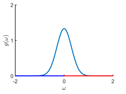
a b

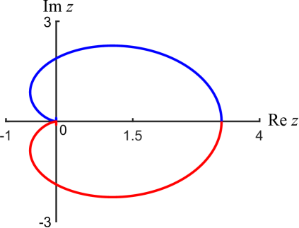
Figure 1: A unimodal probability density function $g$ (a) and the corresponding critical curve (b).

Proof of Theorem 3.6.

Let $\mu>0$ be an eigenvalue of $\boldsymbol{W}$. Note that $\mathcal{C}=\mathcal{D}({\mathrm{i}\mkern 1.0mu}\mathbb{R})$ is a bounded closed curve intersecting positive real semiaxis at a single point $(g_{0},0)$ by Lemma 3.9. Since $\mathcal{D}(\lambda)$ is holomorphic in $\mathbb{H}_{0}$, by the Argument Principle, the eigenequation

$$\mathcal{D}(\lambda)=(K\mu)^{-1}$$ (3.28)

has a root in $\mathbb{H}_{0}$ if the winding number of $\mathcal{D}$ about $(K\mu)^{-1}$ is positive. Therefore, (3.28) has no roots in $\mathbb{H}_{0}$ for $0<K\mu<g_{0}^{-1}$ for any $\mu\in\sigma_{p}(\boldsymbol{W})\backslash\{0\}$, i.e., for $K\in[0,K_{c})$ with $K_{c}=(\mu_{max}g_{0})^{-1}$. Since $g(\omega)$ is an even function, $\mathcal{D}({\mathrm{i}\mkern 1.0mu}\mathbb{R})$ intersects positive real semiaxis when $\lambda=0$. This implies that $g_{0}=\lambda(0)$, which is obtained from (3.25) as

$$\lim_{y\to 0}\lim_{x\to 0+}\mathcal{D}(x+{\mathrm{i}\mkern 1.0mu}y) = \pi g(0)+{\mathrm{i}\mkern 1.0mu}\cdot\operatorname{p.v.}\int_{\mathbb{R}}\frac{g(s)}{s}ds-\int_{\mathbb{R}}\frac{1+{\mathrm{i}\mkern 1.0mu}s}{1+s^{2}}g(s)ds$$

$$= \pi g(0)-\int_{\mathbb{R}}\frac{1}{1+s^{2}}g(s)ds.$$

This proves the first statement of the theorem with formulae (3.22) and (3.23).

Since $\mathcal{D}^{\prime}(0)\neq 0$ by Lemma 3.9 and $\mathcal{D}$ is holomorphic at $0$, it is locally invertible, and the inverse is a holomorphic function. By differentiating both sides of (3.28) with respect to $K$, we have

$$\lambda^{\prime}(K_{c})=\frac{-1}{\mu_{\max}K^{2}_{c}\mathcal{D}^{\prime}(0)}>0.$$

Since $\mu_{max}$ is an isolated eigenvalue of $\boldsymbol{W}$, there are no other roots of (3.28) for $K\in(K_{c}-\epsilon,K_{c}+\epsilon)$. ∎

Proof of Lemma 3.9.

Equation (3.25) follows from the Sokhotski–Plemelj formula [12]. Equation (3.26) follows from (3.25), because $g\in L^{1}(\mathbb{R})$. To show (3.27), note first

$$\begin{split}\mathcal{D}^{\prime}(\lambda)&=-\int_{\mathbb{R}}\left(\frac{1}{(\lambda-{\mathrm{i}\mkern 1.0mu}s)^{2}}-\frac{1}{(\lambda+1-{\mathrm{i}\mkern 1.0mu}s)^{2}}\right)g(s)ds\\ &=-{\mathrm{i}\mkern 1.0mu}\int_{\mathbb{R}}\left(\frac{1}{\lambda-{\mathrm{i}\mkern 1.0mu}s}-\frac{1}{\lambda+1-{\mathrm{i}\mkern 1.0mu}s}\right)g^{\prime}(s)ds.\end{split}$$ (3.29)

Using the Sokhotski–Plemelj formula again, from (3.29) we get

$$\lim_{\lambda\to 0+}D^{\prime}(\lambda)=\operatorname{p.v.}\int_{\mathbb{R}}\frac{g^{\prime}(s)}{s}ds+{\mathrm{i}\mkern 1.0mu}\left(\int_{\mathbb{R}}\frac{1}{1-{\mathrm{i}\mkern 1.0mu}s}g^{\prime}(s)ds-\pi g^{\prime}(0)\right).$$ (3.30)

Since $g^{\prime}$ is an odd function, we have

$$\begin{split}\lim_{\lambda\to 0+}D^{\prime}(\lambda)&=\lim_{\varepsilon\to 0+}\int^{\infty}_{\varepsilon}\frac{g^{\prime}(s)-g^{\prime}(-s)}{s}ds-\int_{\mathbb{R}}\frac{sg^{\prime}(s)}{1+s^{2}}ds\\ &=2\lim_{\varepsilon\to 0+}\int^{\infty}_{\varepsilon}\frac{g^{\prime}(s)}{s}ds-2\int^{\infty}_{0}\frac{sg^{\prime}(s)}{1+s^{2}}ds\\ &=2\lim_{\varepsilon\to 0+}\int^{\infty}_{\varepsilon}\frac{g^{\prime}(s)}{s(1+s^{2})}ds<0,\end{split}$$

where we used that $g^{\prime}(s)\leq 0$ for $s>0$ and is not everywhere zero on $\mathbb{R}^{+}$ to obtain the last inequality.

Finally, (3.26) implies that $\mathcal{C}$ is a bounded closed curve. From (3.25), for $\mathcal{G}(y)=\lim_{x\to 0+}\mathcal{D}(x+{\mathrm{i}\mkern 1.0mu}y)$ we have

$$\Re\mathcal{G}(y) = \pi g(y)-\int_{\mathbb{R}}\frac{g(s)}{1+(y-s)^{2}}ds,$$ (3.31)

$$\Im\mathcal{G}(y) = \int_{\mathbb{R}}\frac{(y-s)g(s)}{1+(y-s)^{2}}ds-\operatorname{p.v.}\int_{\mathbb{R}}\frac{g(s)}{y-s}ds.$$ (3.32)

Here, $\Re z$ and $\Im z$ stand for the real and imaginary parts of $z\in\mathbb{C}$ respectively. Using even symmetry of $g$, from (3.31) and (3.32) it follows that $(g_{0},0)$ is a point of intersection of $\mathcal{C}$ with the positive semiaxis (Figure 1b). Even symmetry and unimodality of $g$ provides the uniqueness:

$$\begin{split}-\Im D(x+{\mathrm{i}\mkern 1.0mu}y)&=\int_{\mathbb{R}}\left(\frac{y-\omega}{x^{2}+(y-\omega)^{2}}-\frac{y-\omega}{(x+1)^{2}+(y-\omega)^{2}}\right)g(\omega)d\omega\\ &=-\int_{\mathbb{R}}\left(\frac{\omega}{x^{2}+\omega^{2}}-\frac{\omega}{(x+1)^{2}+\omega^{2}}\right)g(y+\omega)d\omega\\ &=-\left\{\int_{-\infty}^{0}+\int_{0}^{\infty}\right\}\left(\frac{\omega}{x^{2}+\omega^{2}}-\frac{\omega}{(x+1)^{2}+\omega^{2}}\right)g(y+\omega)d\omega\\ &=-\int_{0}^{\infty}\left(\frac{\omega}{x^{2}+\omega^{2}}-\frac{\omega}{(x+1)^{2}+\omega^{2}}\right)g(y+\omega)d\omega\\ &+\int_{0}^{\infty}\left(\frac{\omega}{x^{2}+\omega^{2}}-\frac{\omega}{(x+1)^{2}+\omega^{2}}\right)g(y-\omega)d\omega\\ &=-\int_{0}^{\infty}\frac{\omega\left((x+1)^{2}-x^{2}\right)}{(x^{2}+\omega^{2})\left((x+1)^{2}+\omega^{2}\right)}\left(g(y+\omega)-g(y-\omega)\right)d\omega.\end{split}$$ (3.33)

Even symmetry of $g$ implies that $y=0$ solves $\Im D(x+{\mathrm{i}\mkern 1.0mu}y)=0$ (cf. (3.33)). For unimodal $g$ this solution is unique, because in this case $g(y+\omega)-g(y-\omega)>0$ when $y<0,\;\omega>0$ and $g(y+\omega)-g(y-\omega)<0$ when $y>0,\;\omega>0$.

∎

3.4 The resolvent and the Riesz projector

In this section, we compute the resolvent operator

$$\boldsymbol{R}_{\lambda}=\left(\lambda-\boldsymbol{S}\right)^{-1}$$

and the Riesz projector for $\boldsymbol{S}$.

Lemma 3.10.

For $\phi\in\mathcal{H}_{0}^{+}$,

$$\boldsymbol{R}_{\lambda}\phi=\left(\lambda-\boldsymbol{L}_{1}\right)^{-1}\phi+KD(\lambda;\xi,\eta)\left(\boldsymbol{I}-KD(\lambda)\boldsymbol{W}\right)^{-1}\boldsymbol{W}\left[\left(\left(\lambda-\boldsymbol{L}_{1}\right)^{-1}\phi\right)(0,0,\cdot)\right].$$ (3.34)

Proof.

From the definitions of $\boldsymbol{R}_{\lambda}$ and $\boldsymbol{S}$ we have

$$\left(\lambda-\boldsymbol{L}_{1}-K\boldsymbol{B}\right)\boldsymbol{R}_{\lambda}\phi=\phi\quad\forall\phi\in\mathcal{H}_{0}^{+}.$$ (3.35)

We rewrite (3.35) as

$$\left(\lambda-\boldsymbol{L}_{1}\right)\left(\boldsymbol{I}-K\left(\lambda-\boldsymbol{L}_{1}\right)^{-1}\boldsymbol{B}\right)\boldsymbol{R}_{\lambda}\phi=\phi.$$

Thus, (3.15) gives

$$\boldsymbol{R}_{\lambda}\phi =\left(\lambda-\boldsymbol{L}_{1}\right)^{-1}\phi+K\left(\lambda-\boldsymbol{L}_{1}\right)^{-1}\boldsymbol{B}\boldsymbol{R}_{\lambda}\phi$$

$$=\left(\lambda-\boldsymbol{L}_{1}\right)^{-1}\phi+KD(\lambda;\xi,\eta)\boldsymbol{W}\left[(\boldsymbol{R}_{\lambda}\phi)(0,0,\cdot)\right].$$ (3.36)

By setting $\xi=\eta=0$ and applying $\boldsymbol{W}$ to both sides of (3.36), after some algebra we obtain

$$\boldsymbol{W}\left[(\boldsymbol{R}_{\lambda}\phi)(0,0,\cdot)\right]=\left(\boldsymbol{I}-KD(\lambda)\boldsymbol{W}\right)^{-1}\boldsymbol{W}\left[\left(\left(\lambda-\boldsymbol{L}_{1}\right)^{-1}\phi\right)(0,0,\cdot)\right].$$ (3.37)

By plugging (3.37) into (3.36), we obtain (3.34). ∎

From (3.34) one can see that the spectrum of $\boldsymbol{S}$, as an operator on $\mathcal{H}^{+}_{0}$, is the union of the residual spectrum of $\boldsymbol{L}_{1}$ and point spectrum of $\boldsymbol{S}$ coming from the factor $\left(\boldsymbol{I}-KD(\lambda)\boldsymbol{W}\right)^{-1}$;

$$\sigma(\boldsymbol{S})=\sigma(\boldsymbol{L}_{1})\bigcup\sigma_{p}(\boldsymbol{S}).$$

Although $\{z\in\mathbb{C}:\;-1\leq\Re z\leq 0\}$ is a residual spectrum of $\boldsymbol{L}_{1}$, as shown in Section 3.3, $D(\lambda;\xi,\eta)$ and $D(\lambda)$ have the analytic continuations from $\mathbb{H}_{0}$ to $\mathbb{H}_{a}$ denoted by $\mathcal{D}(\lambda;\xi,\eta)$ and $\mathcal{D}(\lambda)$, respectively. Recall that $\mathcal{D}(\lambda;\xi,\eta)\in\mathcal{Y}_{a}^{-}$ when $\hat{g}\in\mathcal{X}^{+}_{a}$. In a similar manner, we can verify that $\left(\lambda-\boldsymbol{L}_{1}\right)^{-1}$ has an analytic continuation from $\mathbb{H}_{0}$ to $\mathbb{H}_{a}$ as an operator from $\mathcal{H}_{a}^{+}$ to $\mathcal{H}_{a}^{-}$. Using them, we define the analytic continuation of $\boldsymbol{R}_{\lambda}$ from $\mathbb{H}_{0}$ to $\mathbb{H}_{a}$ by

$$\mathcal{R}_{\lambda}\phi=\left(\lambda-\boldsymbol{L}_{1}\right)^{-1}\phi+K\mathcal{D}(\lambda;\xi,\eta)\left(\boldsymbol{I}-K\mathcal{D}(\lambda)\boldsymbol{W}\right)^{-1}\boldsymbol{W}\left[\left(\left(\lambda-\boldsymbol{L}_{1}\right)^{-1}\phi\right)(0,0,\cdot)\right].$$ (3.38)

This is an operator from $\mathcal{H}_{a}^{+}$ into $\mathcal{H}_{a}^{-}$ called the generalized resolvent. Note that the generalized eigenvalues in Definition 3.4 are the poles of $\mathcal{R}_{\lambda}$. Recall the definitions of the Banach spaces $\mathcal{H}^{\pm}_{a}$ and $\mathcal{H}^{\pm}_{0}$ (cf. (3.2)) and note that they form Gelfand triplet:

$$\mathcal{H}^{+}_{a}\subset\mathcal{H}^{+}_{0}=\mathcal{H}^{-}_{0}\subset\mathcal{H}^{-}_{a}.$$

For the analytic continuation, the domain of $\mathcal{R}_{\lambda}$ is restricted to $\mathcal{H}^{+}_{a}$ and the range is extended to $\mathcal{H}^{-}_{a}$.

The corresponding generalized Riesz projection $\mathcal{P}_{\lambda}:\mathcal{H}^{+}_{a}\rightarrow\mathcal{H}^{-}_{a}$ is given by

$$\mathcal{P}_{\lambda}\phi=\frac{1}{2\pi{\mathrm{i}\mkern 1.0mu}}\oint_{c}\mathcal{R}_{z}\phi dz,$$ (3.39)

where $c$ is a positively oriented closed curve, which encircles an eigenvalue $\lambda$ but no other generalized eigenvalues. Note that the generalized eigenfunction corresponding to $\lambda$ in Definition 3.4 is an element of the image $\mathcal{P}_{\lambda}$. We conclude this section with the computation of the generalized Riesz projection for the bifurcating eigenvalue $\lambda=0$:

$$\mathcal{P}_{0}[\phi]=\frac{1}{2\pi{\mathrm{i}\mkern 1.0mu}}\oint_{c}\mathcal{R}_{z}\phi dz,$$ (3.40)

where $c$ is a positively oriented contour around the origin, which does not contain any other generalized eigenvalues of $\boldsymbol{S}$.

Here and in the remainder of this paper, we suppress the subscript of $\mathcal{P}_{0}$ since from now on we will only be interested in the bifurcating eigenvalue. Further, suppose that $\mu_{max}$, the largest positive eigenvalue of $\boldsymbol{W}$, is simple. The Riesz projection for $\boldsymbol{W}$ corresponding to $\mu_{max}$ is denoted by

$$\boldsymbol{P}[\Phi]=\frac{1}{2\pi{\mathrm{i}\mkern 1.0mu}}\oint_{C}\left(z-\boldsymbol{W}\right)^{-1}\Phi dz,$$ (3.41)

where $C$ is a positively oriented contour around $\mu_{max}$, which does not contain any other eigenvalues of $\boldsymbol{W}$.

Lemma 3.11.

$$\mathcal{P}[\phi](\xi,\eta,x)=\rho_{1}\mathcal{D}(0;\xi,\eta)\boldsymbol{P}[\Phi](0,0,x),$$ (3.42)

where $\Phi:=\lim_{\lambda\to 0+}\left(\lambda-\boldsymbol{L}_{1}\right)^{-1}\phi$ and $\rho_{1}>0$.

Proof.

First, note

$$\mathcal{R}_{\lambda}[\phi](\xi,\eta,x)=\Phi_{\lambda}(\xi,\eta,x)+K\mathcal{D}(\lambda;\xi,\eta)\left(\boldsymbol{I}-K\mathcal{D}(\lambda)\boldsymbol{W}\right)^{-1}\boldsymbol{W}\left[\Phi_{\lambda}(0,0,\cdot)\right](x),$$ (3.43)

where

$$\Phi_{\lambda}:=\left(\lambda-\boldsymbol{L}_{1}\right)^{-1}\phi.$$ (3.44)

Using (3.43), we have

$$\oint_{c}\mathcal{R}_{z}[\phi](\xi,\eta,x)dz=K\oint_{c}\mathcal{D}(z;\xi,\eta)\left(\boldsymbol{I}-K\mathcal{D}(z)\boldsymbol{W}\right)^{-1}\boldsymbol{W}[\Phi_{z}(0,0,\cdot)](x)dz,$$ (3.45)

where we used $\oint_{c}\Phi_{z}(\xi,\eta,x)dz=0,$ because $\Phi_{z}(\xi,\eta,x)$ is regular inside $c$. By continuity $\mathcal{D}^{\prime}(z)\neq 0$ on $c$ provided $c$ is sufficiently small. Change variable in (3.45) to $z:=z(\alpha)$ such that

$$\alpha=\left(K\mathcal{D}(z)\right)^{-1}.$$ (3.46)

Note that

$$\mu_{max}=\left(K_{c}\mathcal{D}(0)\right)^{-1},$$ (3.47)

as follows from (3.21). We have

$$\begin{split}\oint_{c}\mathcal{R}_{z}[\phi](\xi,\eta,x)dz&=-\displaystyle\oint_{C}\frac{\mathcal{D}\left(z(\alpha);\xi,\eta\right)}{\alpha^{2}\mathcal{D}^{\prime}\left(z(\alpha)\right)}\boldsymbol{W}(\boldsymbol{I}-\alpha^{-1}\boldsymbol{W})^{-1}[\Phi_{z(\alpha)}](0,0,x)d\alpha\\ &=-\oint_{C}\frac{\mathcal{D}(z(\alpha);\xi,\eta)}{\alpha\mathcal{D}^{\prime}\left(z(\alpha)\right)}\boldsymbol{W}(\alpha-\boldsymbol{W})^{-1}\left[\Phi_{z(\alpha)}\right](0,0,x)d\alpha,\end{split}$$ (3.48)

where $C$ stands for the image of $c$ under (3.46). Since $\mu_{max}$ is a simple eigenvalue of $\boldsymbol{W}$, $\left(\alpha-\boldsymbol{W}\right)^{-1}$ has a simple pole $\alpha=\mu_{max}$ inside $C$ while the other factor under the integral is regular. Thus, (3.48) yields

$$\oint_{c}\mathcal{R}_{z}[\phi](\xi,\eta,x)dz=\frac{-\mathcal{D}(0;\xi,\eta)}{\mu_{max}\mathcal{D}^{\prime}(0)}\boldsymbol{W}\oint_{C}\left(\alpha-\boldsymbol{W}\right)^{-1}\left[\Phi\right](0,0,x)d\alpha.$$ (3.49)

Noting that the integral on the right–hand side implements Riesz projection of $\boldsymbol{W}$ for $\mu_{max}$, we further have

$$\begin{split}\frac{1}{2\pi{\mathrm{i}\mkern 1.0mu}}\oint_{c}\mathcal{R}_{z}[\phi](\xi,\eta,x)dz&=\frac{-\mathcal{D}(0;\xi,\eta)}{\mu_{max}\mathcal{D}^{\prime}(0)}\boldsymbol{W}\frac{1}{2\pi{\mathrm{i}\mkern 1.0mu}}\oint_{C}\left(\alpha-\boldsymbol{W}\right)^{-1}\left[\Phi\right](0,0,x)d\alpha\\ &=\frac{-\mathcal{D}(0;\xi,\eta)}{\mu_{max}\mathcal{D}^{\prime}(0)}\boldsymbol{W}\boldsymbol{P}\left[\Phi\right](0,0,x)\\ &=\rho_{1}\mathcal{D}(0;\xi,\eta)\boldsymbol{P}\left[\Phi\right](0,0,x),\end{split}$$ (3.50)

where $\rho_{1}=-\left(\mathcal{D}^{\prime}(0)\right)^{-1}>0$ by Lemma 3.9. ∎

3.5 Asymptotic stability

We conclude this section with an application to linear asymptotic stability of mixing. For $K\in[0,K_{c}),$ $\boldsymbol{S}$ has no eigenvalues, nonetheless mixing is asymptotically stable in the appropriate topology.

Theorem 3.12.

Suppose Assumption 2.1 holds. Then for $K\in[0,K_{c})$ the mixing state is linearly asymptotically stable under the perturbations from $\mathcal{H}^{+}_{a}\subset\mathcal{H}^{-}_{a}$ in the topology of $\mathcal{H}^{-}_{a}$.

Proof.

We estimate the semigroups of the linearized systems (2.13), (2.14). Each of the operators $\boldsymbol{L}_{j},\,j\geq 1,$ generates a continuous semigroup on $\mathcal{H}_{a}^{+}\subset\mathcal{H}_{a}^{-}$ in the topology of $\mathcal{H}^{-}_{a}$:

$$e^{\boldsymbol{L}_{j}t}[\phi](\xi,\eta,x) =\phi(\xi+t,\eta+jt,x),\quad j\geq 1,$$ (3.51)

$$\lim_{t\to\infty}\|e^{\boldsymbol{L}_{j}t}[\phi](t)\|_{\mathcal{H}_{a}^{-}} =0.$$

For $\boldsymbol{L}_{0}$, the same statement holds because of the constraint $w_{0}(t,\infty,\eta,x)=0$.

Since $\boldsymbol{B}$ is a bounded operator, $\boldsymbol{S}$ generates a continuous semigroup expressed by the Laplace inversion formula for $\phi\in\mathcal{H}_{a}^{+}$:

$$\begin{split}e^{\boldsymbol{S}t}[\phi](\xi,\eta,x)&=\frac{1}{2\pi{\mathrm{i}\mkern 1.0mu}}\lim_{c\to\infty}\int^{b+{\mathrm{i}\mkern 1.0mu}c}_{b-{\mathrm{i}\mkern 1.0mu}c}\!e^{\lambda t}\mathcal{R}_{\lambda}[\phi](\xi,\eta,x)d\lambda\end{split}$$ (3.52)

for some positive $b$. Let $K\in[0,K_{c})$ be arbitrary but fixed. By Theorem 3.6, there exists $\epsilon>0$ such that there are no generalized eigenvalues in $\{-\epsilon\leq\Re z\}$ and the generalized resolovent $\mathcal{R}_{\lambda}$ is holomorphic in this region. Hence, the integral pass can be moved to the left half plane and we obtain

$$\begin{split}e^{\boldsymbol{S}t}[\phi](\xi,\eta,x)&=\frac{1}{2\pi{\mathrm{i}\mkern 1.0mu}}\lim_{c\to\infty}\int^{-\epsilon+{\mathrm{i}\mkern 1.0mu}c}_{-\epsilon-{\mathrm{i}\mkern 1.0mu}c}\!e^{\lambda t}\mathcal{R}_{\lambda}[\phi](\xi,\eta,x)d\lambda\\ &=\frac{e^{-\varepsilon t}}{2\pi{\mathrm{i}\mkern 1.0mu}}\lim_{c\to\infty}\int^{c}_{-c}\!{\mathrm{i}\mkern 1.0mu}e^{{\mathrm{i}\mkern 1.0mu}\lambda t}\mathcal{R}_{i\lambda-\epsilon}[\phi](\xi,\eta,x)d\lambda\rightarrow 0\end{split}$$ (3.53)

in $\mathcal{H}^{-}_{a}$ as $t\to\infty$. ∎

4 The pitchfork bifurcation

In this section, we study a pitchfork bifurcation of mixing underlying the onset of synchronization in the second order KM. This bifurcation is identified as the point in the parameter space at which a generalized eigenvalue crosses the imaginary axis. Its analysis requires generalized spectral theory [2].

4.1 Assumptions and the main result

Throughout this section, we assume the following

(A-1)

$\mu_{max}>0$ is a simple eigenvalue of $\boldsymbol{W}$ with the corresponding eigenfunction $V_{max}$;

(A-2)

$g$ is an even unimodal probability density function subject to Assumption 2.1.

Assumption (A-1) holds for many common graph sequences encountered in applications including all–to–all, Erdős–Rényi, small–world graphs, to name a few [3]. Assumption (A-2) covers the most representative case. It can be relaxed. We impose it for simplicity.

Remark 4.1.

Suppose $\boldsymbol{W}$ has negative eigenvalues. Denote the smallest negative eigenvalue $\mu_{min}$ and assume that it is simple with the corresponding eigenfunction $V_{min}$. Then after setting $W:=-W$ and $K:=-K$, we find that the resultant system satisfies (A) and the analysis below shows that the original system undergoes a pitchfork bifurcation at $K_{c}^{-}=(g_{0}\mu_{min})^{-1}<0$.

Under these assumptions, as follows from the analysis in Section 3, at $K=K_{c}$, $\boldsymbol{S}$ has a simple generalized eigenvalue $\lambda=0$. The corresponding eigenfunction is (cf. (3.19))

$$v_{0}=K_{c}\lim_{\lambda\to 0+}D(\lambda(\mu_{max});\xi,\eta)V_{max}\in\mathcal{H}^{-}_{a}.$$ (4.1)

Finally, we postulate the existence of a one–dimensional center manifold for the vector field in (2.12) for $K=K_{c}$. As we already stated in the Introduction, the proof of this fact is a very technical problem, which is not addressed in this paper. The proof of existence of a center manifold in the classical KM can be found in [1].

In the remainder of this section, we perform a center manifold reduction and show that at $K=K_{c}$, the system undergoes a pitchfork bifurcation. The branch of stable steady state solutions bifurcating from mixing is given in terms of the corresponding values of the order parameter:

$$|h_{\infty}(x)|=K_{c}^{-2}(\mu_{max}\rho_{2}\rho_{3}(x))^{-1/2}\sqrt{K-K_{c}}+O(K-K_{c}),$$ (4.2)

where $\rho_{2}>0$ and $\rho_{3}(x)$ are defined below. In many applications, $\rho_{3}(x)\equiv 1$ (see Remark 4.3 for more details).

4.2 The center manifold reduction

The existence of the one–dimensional center manifold at $K=K_{c}$ implies the following Ansatz for the solutions of (2.12) with $K=K_{c}+\epsilon^{2}$, $0<\epsilon\ll 1$:

$$w_{1} = \mathcal{P}w_{1}+(\boldsymbol{I}-\mathcal{P})w_{1}=\epsilon c(t)v_{0}+O(\epsilon^{2}),$$ (4.3)

$$w_{k} = q_{k}(w_{1}),\;k\in\mathbb{N}_{1}:=\{0\}\bigcup\{2,3,\dots\},$$ (4.4)

where $\mathcal{P}$ is the Riesz projector (cf. (3.40)), $c(t)$ is the function determining the location on the slow manifold, and $q_{k},k\in\mathbb{N}_{1},$ are smooth functions such that $q_{k}(0)=q^{\prime}_{k}(0)=0$.

Using the Ansatz (4.3) and (4.4), below we derive (4.2). Let $K=K_{c}+\epsilon^{2}$ and rewrite equations for $w_{0}$, $w_{1}$, and $w_{2}$ in (2.12) as follows

$$\partial_{t}w_{0} = \partial_{\xi_{0}}w_{0}-Ke^{-\xi_{0}}\left(h(t,x)w_{-1}-\overline{h(t,x)}w_{1}\right),$$ (4.5)

$$\partial_{t}w_{1} = \boldsymbol{S}_{0}w_{1}+\epsilon^{2}\left(1-e^{-\xi_{1}}\right)h(t,x)\hat{g}(\eta)$$

$$+ K\left(1-e^{-\xi_{1}}\right)\left(h(t,x)w_{0}-\overline{h(t,x)}w_{2}\right),$$

$$\partial_{t}w_{2} = \partial_{\xi_{2}}w_{2}+2\partial_{\eta}w_{2}+K(2-e^{-\xi_{2}})\left(h(t,x)w_{1}-\overline{h(t,x)}w_{3}\right),$$ (4.7)

where $\xi_{i},\;i\in\mathbb{N},$ are as defined in (2.9), and $\boldsymbol{S}_{0}$ is defined by setting $K=K_{c}$ in the expression for $\boldsymbol{S}$ (cf. (2.13)). In particular,

$$\boldsymbol{S}w_{1}=\boldsymbol{S}_{0}w_{1}+\epsilon^{2}\left(1-e^{-\xi_{1}}\right)h(t,x)\hat{g}(\eta).$$ (4.8)

Lemma 4.2.

Let

$$P_{0}(\lambda;\xi_{1},\omega) = \frac{e^{-\xi_{1}}-1}{\lambda-{\mathrm{i}\mkern 1.0mu}\omega}-\frac{e^{-\xi_{1}}-1}{\lambda+{\mathrm{i}\mkern 1.0mu}\omega}-\frac{e^{-\xi_{1}}-1}{\lambda+1-{\mathrm{i}\mkern 1.0mu}\omega}-\frac{1}{2}\frac{(e^{-\xi_{1}}-1)^{2}}{\lambda+1-{\mathrm{i}\mkern 1.0mu}\omega}$$

$$+ \frac{e^{-\xi_{1}}-1}{\lambda+1+{\mathrm{i}\mkern 1.0mu}\omega}-\frac{1}{2}\frac{(e^{-\xi_{1}}-1)^{2}}{\lambda+1+{\mathrm{i}\mkern 1.0mu}\omega},$$

$$P_{2}(\lambda;\xi_{1},\omega) = \frac{1}{(\lambda-{\mathrm{i}\mkern 1.0mu}\omega)^{2}}+\frac{1}{2}\frac{(e^{-\xi_{1}}+1)^{2}}{(\lambda+1-{\mathrm{i}\mkern 1.0mu}\omega)^{2}}+\frac{1}{\lambda-{\mathrm{i}\mkern 1.0mu}\omega}-\frac{1}{\lambda+1-{\mathrm{i}\mkern 1.0mu}\omega}$$

$$- \frac{e^{-\xi_{1}}+1}{\lambda-{\mathrm{i}\mkern 1.0mu}\omega}-\frac{2(e^{-\xi_{1}}+1)}{\lambda+1/2-{\mathrm{i}\mkern 1.0mu}\omega}+\frac{3(e^{-\xi_{1}}+1)}{\lambda+1-{\mathrm{i}\mkern 1.0mu}\omega},$$

$$P_{1}(\lambda;\xi_{1},\eta) = \int_{\mathbb{R}}\left(\lambda-\boldsymbol{L}_{1}\right)^{-1}\left[\left(1-e^{-\xi_{1}}\right)\left(P_{0}-P_{2}\right)e^{{\mathrm{i}\mkern 1.0mu}\eta\omega}\right]g(\omega)d\omega.$$ (4.11)

On the center manifold, we have

$$h(t,x) = \epsilon c(t)V_{max}(x)+O(\epsilon^{2}),$$ (4.12)

$$w_{0} = K_{c}^{2}\epsilon^{2}|c(t)|^{2}|V_{max}|^{2}\lim_{\lambda\to 0+}\int_{\mathbb{R}}P_{0}(\lambda;\xi_{1},\omega)e^{{\mathrm{i}\mkern 1.0mu}\eta\omega}g(\omega)d\omega+O(\epsilon^{3}),$$ (4.13)

$$w_{2} = K_{c}^{2}\epsilon^{2}c(t)^{2}V_{max}^{2}\lim_{\lambda\to 0+}\int_{\mathbb{R}}P_{2}(\lambda;\xi_{1},\omega)e^{{\mathrm{i}\mkern 1.0mu}\eta\omega}g(\omega)d\omega+O(\epsilon^{3}).$$ (4.14)

In addition,

$$\rho_{2}=-\lim_{\lambda\to 0+}P_{1}(\lambda;0,0)>0.$$ (4.15)

The number $\rho_{2}$ is determined solely by $g(\omega)$. Its expression will be given in the end of Sec.4.3. With Lemma 4.2 in hand, we now turn to the center manifold reduction. The proof of the lemma is given in the next subsection.

We want to project both sides of (4.2) onto the eigenspace spanned by $v_{0}$. To this end, we note

$$\mathcal{P}[{\partial}_{t}w_{1}]=\epsilon\dot{c}(t)v_{0},\quad\mbox{and}\quad\mathcal{P}[\boldsymbol{S}_{0}w_{1}]=0,$$ (4.16)

as follows from (4.3). Further, from Lemma 3.11,

$$\mathcal{P}\left[\left(1-e^{-\xi_{1}}\right)h(t,x)\hat{g}(\eta)\right]=\rho_{1}\lim_{\lambda\to 0+}\left\{\mathcal{D}(\lambda;\xi_{1},\eta)\left.\boldsymbol{P}\left[\left(\lambda-\boldsymbol{L}_{1}\right)^{-1}\left(1-e^{-\xi_{1}}\right)\hat{g}(\eta)h(t,x)\right]\ \right|_{\xi_{1}=\eta=0}\right\}.$$ (4.17)

By the first line in (3.15),

$$\left(\lambda-\boldsymbol{L}_{1}\right)^{-1}\left(1-e^{-\xi_{1}}\right)\hat{g}(\eta)=\mathcal{D}(\lambda;\xi_{1},\eta).$$ (4.18)

After plugging (4.18) and (4.12) into (4.17), we have

$$\begin{split}\mathcal{P}\left[\left(1-e^{-\xi_{1}}\right)h(t,x)\hat{g}(\eta)\right]&=\rho_{1}\lim_{\lambda\to 0+}\left\{\mathcal{D}(\lambda;\xi_{1},\eta)\boldsymbol{P}\left[\mathcal{D}(\lambda;\xi_{1},\eta)h(t,x)\right]_{\xi_{1}=\eta=0}\right\}\\ &=\rho_{1}\lim_{\lambda\to 0+}\left\{\mathcal{D}(\lambda;\xi_{1},\eta)\mathcal{D}(\lambda)\right\}\boldsymbol{P}\left[\epsilon c(t)V_{max}\right](0,0,x)+O(\epsilon^{2})\\ &=\epsilon\rho_{1}c(t)V_{max}(x)\lim_{\lambda\to 0+}\left\{\mathcal{D}(\lambda;\xi_{1},\eta)\mathcal{D}(\lambda)\right\}+O(\epsilon^{2})\\ &=\frac{\epsilon\rho_{1}c(t)v_{0}}{K_{c}^{2}\mu_{max}}+O(\epsilon^{2}),\end{split}$$ (4.19)

where we used (3.47) and (4.1) to obtain the last equality.

Finally, we turn to the last group of terms of the right–hand side of (4.2). By Lemma 4.2,

$$\begin{split}h(t,x)w_{0}-\overline{h(t,x)}w_{2}&=\epsilon^{3}K_{c}^{2}c(t)|c(t)|^{2}V_{max}|V_{max}|^{2}\times\\ &\times\lim_{\lambda\to 0+}\int_{\mathbb{R}}\left[P_{0}-P_{2}\right](\lambda;\xi_{1},\omega)e^{{\mathrm{i}\mkern 1.0mu}\eta\omega}g(\omega)d\omega+O(\epsilon^{4}).\end{split}$$ (4.20)

Further,

$$\begin{split}\left(\lambda-\boldsymbol{L}_{1}\right)^{-1}\left[(1-e^{-\xi_{1}})\left(hw_{0}-\overline{h}w_{2}\right)\right]&=\epsilon^{3}K_{c}^{2}c(t)|c(t)|^{2}V_{max}|V_{max}|^{2}\lim_{\lambda\to 0+}P_{1}(\lambda;\xi_{1},\eta)\\ &+O(\epsilon^{4}),\end{split}$$ (4.21)

where $P_{1}$ is defined in (4.11). This yields

$$\begin{split}\mathcal{P}\left[(1-e^{-\xi_{1}})\left(hw_{0}-\overline{h}w_{2}\right)\right]&=\rho_{1}\lim_{\lambda\to 0+}\left\{\mathcal{D}(\lambda;\xi_{1},\eta)\boldsymbol{P}\left[\left(\lambda-\boldsymbol{L}_{1}\right)^{-1}\left(1-e^{-\xi_{1}}\right)\left(hw_{0}-\bar{h}w_{2}\right)\right]_{\xi_{1}=\eta=0}\right\}\\ &=\epsilon^{3}\rho_{1}K_{c}^{2}c(t)|c(t)|^{2}\lim_{\lambda\to 0+}\left\{\mathcal{D}(\lambda;\xi_{1},\eta)\boldsymbol{P}\left[V_{max}|V_{max}|^{2}\right]P_{1}(\lambda;0,0)\right\}+O(\epsilon^{4})\\ &=\epsilon^{3}\rho_{1}K_{c}c(t)|c(t)|^{2}v_{0}\frac{\boldsymbol{P}\left[V_{max}|V_{max}|^{2}\right]}{V_{max}}\lim_{\lambda\to 0+}P_{1}(\lambda;0,0)+O(\epsilon^{4}).\end{split}$$ (4.22)

By projecting both sides of (4.2) onto the subspace spanned by $v_{0}$ and using (4.16), (4.19), and (4.22), we obtain

$$\epsilon\dot{c}v_{0}=\frac{\epsilon^{3}\rho_{1}}{K_{c}^{2}\mu_{max}}c(t)v_{0}+\epsilon^{3}K_{c}^{2}\rho_{1}c(t)|c(t)|^{2}v_{0}\frac{\boldsymbol{P}[V_{max}|V_{max}|^{2}]}{V_{max}}\lim_{\lambda\to 0+}P_{1}(\lambda;0,0)+O(\epsilon^{4}).$$

This yields

$$\dot{c}=\frac{\epsilon^{2}\rho_{1}}{K_{c}^{2}\mu_{max}}c(t)\left(1+K_{c}^{4}\mu_{max}\lim_{\lambda\to 0+}P_{1}(\lambda;0,0)\frac{\boldsymbol{P}[V_{max}|V_{max}|^{2}]}{V_{max}}|c(t)|^{2}\right)+O(\epsilon^{3}).$$ (4.23)

Equation (4.23) describes the dynamics on the center manifold. Recalling that $h(t,x)=\epsilon c(t)V_{max}+O(\epsilon^{2})$ from Lemma 4.2, we rewrite this equation to the equation of the local order parameter $h=h(t,x)$ as

$$\frac{dh}{dt} = \frac{\rho_{1}}{K_{c}^{2}\mu_{max}}h\left(\epsilon^{2}+K_{c}^{4}\mu_{max}\lim_{\lambda\to 0+}P_{1}(\lambda;0,0)\frac{\boldsymbol{P}[V_{max}|V_{max}|^{2}]}{V_{max}|V_{max}|^{2}}|h|^{2}\right)+O(\epsilon^{4})$$ (4.24)

$$= \frac{\rho_{1}}{K_{c}^{2}\mu_{max}}h\left(\epsilon^{2}-K_{c}^{4}\mu_{max}\rho_{2}\rho_{3}|h|^{2}\right)+O(\epsilon^{4})$$

where $\rho_{2}>0$ is defined in (4.15) and $\rho_{3}$ is defined by

$$\rho_{3}(x):=\frac{\boldsymbol{P}[V_{max}(x)|V_{max}(x)|^{2}]}{V_{max}(x)|V_{max}(x)|^{2}}.$$ (4.25)

Equation (4.24) has a fixed point given by (4.2). It undergoes a pitchfork bifurcation at $K=K_{c}$. Since $\rho_{1}$ and $\rho_{2}$ are positive, the fixed point is stable when $\rho_{3}>0$ (see below).

Remark 4.3.

In many applications, a graphon is of the form $W(x,y)=G(x-y)$ such that $G(x)=G(-x)$. For instance, the family of small-world graphs is defined by the graphon of this type [9, 3]. In this case, $W$ admits Fourier series expansion

$$W(x,y)=\sum_{k\in\mathbb{Z}}c_{k}e^{2\pi{\mathrm{i}\mkern 1.0mu}k(x-y)},\,c_{k}=c_{-k}\in\mathbb{R},\quad\sum_{k\in\mathbb{Z}}c_{k}^{2}<\infty.$$ (4.26)

Then, eigenvalues of the operator $\boldsymbol{W}$ are the coefficients of the expansion. The largest eigenvalue is given by

$$\mu_{max}=c_{m}:=\sup\{c_{k}\,:\,k\in\mathbb{Z}\},$$ (4.27)

and the corresponding eigenfunction is $V_{max}=e^{2\pi{\mathrm{i}\mkern 1.0mu}mx}$ [4]. In this case, $\rho_{3}=1$. For many important graphs such as Erdős–Rényi and small-world graphs, $\mu_{max}=c_{0}$ and $V_{max}=\rho_{3}=1$. In this case, the stable branch of equilibria is given through the values of the order parameter

$$|h_{\infty}(x)|=K_{c}^{-2}(\mu_{max}\rho_{2})^{-1/2}\sqrt{K-K_{c}}+O(K-K_{c}).$$ (4.28)

4.3 Proof of Lemma 4.2

By plugging (4.3) and (4.4) into (4.2) and recalling $\boldsymbol{S}_{0}v_{0}=0$, we immediately get

$$\partial_{t}w_{1}=O(\epsilon^{2}).$$ (4.29)

From this, (4.3) and (4.4), we further observe that

$$\partial_{t}w_{k}=q_{k}^{\prime}(w_{1})\partial_{t}w_{1}=O(\epsilon^{3}),\quad k\in\mathbb{N}_{1}.$$ (4.30)

From (4.3) and the equation for $h$ in (2.12), we have

$$\begin{split}h(t,x)&=\int_{I}\!W(x,y)(\epsilon c(t)v_{0}(0,0,y)+O(\epsilon^{2}))dy\\ &=\epsilon c(t)K_{c}\lim_{\lambda\to 0+}D(\lambda)\int_{I}\!W(x,y)V_{max}(y)dy+O(\epsilon^{2})\\ &=\epsilon c(t)K_{c}\mu_{max}\lim_{\lambda\to 0+}D(\lambda)V_{max}(x)+O(\epsilon^{2})\\ &=\epsilon c(t)V_{max}(x)+O(\epsilon^{2}).\end{split}$$

This shows (4.12).

Next we turn to the equation for $w_{2}$:

$$\partial_{t}w_{2}=\partial_{\xi_{2}}w_{2}+2\partial_{\eta}w_{2}+K(2-e^{-\xi_{2}})(hw_{1}-\overline{h}w_{3}).$$

Since $\partial_{t}w_{2}$ and $\overline{h}w_{3}$ are of order $O(\epsilon^{3})$, we have

$$\left(\partial_{\xi_{2}}+2\partial_{\eta}\right)w_{2}=-K_{c}\epsilon^{2}c(t)^{2}(2-e^{-\xi_{2}})V_{max}v_{0}+O(\epsilon^{3}).$$ (4.31)

Lemma 4.4.

On the center manifold, $w_{2}$ is expressed as

$$w_{2} = K_{c}^{2}\epsilon^{2}c(t)^{2}V_{max}^{2}$$ (4.32)

$$\times \lim_{\lambda\to 0+}\int_{\mathbb{R}}\!\Bigl{(}\frac{1}{(\lambda-{\mathrm{i}\mkern 1.0mu}\omega)^{2}}+\frac{1}{2}\frac{e^{-2\xi_{2}}}{(\lambda+1-{\mathrm{i}\mkern 1.0mu}\omega)^{2}}+\frac{1}{\lambda-{\mathrm{i}\mkern 1.0mu}\omega}-\frac{1}{\lambda+1-{\mathrm{i}\mkern 1.0mu}\omega}$$

$$- \frac{e^{-\xi_{2}}}{\lambda-{\mathrm{i}\mkern 1.0mu}\omega}-\frac{2e^{-\xi_{2}}}{\lambda+1/2-{\mathrm{i}\mkern 1.0mu}\omega}+\frac{3e^{-\xi_{2}}}{\lambda+1-{\mathrm{i}\mkern 1.0mu}\omega}\Bigr{)}e^{i\eta\omega}g(\omega)d\omega+O(\epsilon^{3}).\qquad$$

Proof.

A straightforward substitution shows that (4.32) satisfies (4.31) up to $O(\epsilon)^{3}$. ∎

By the relation $e^{-\xi_{2}}=e^{-\xi_{1}}+1$ derived from (2.9), we obtain (4.14) with (4.2).

Next, the equation for $w_{0}$ is given by

$$\partial_{t}w_{0}=\partial_{\xi_{0}}w_{0}-Ke^{-\xi_{0}}\left(hw_{-1}-\overline{h}w_{1}\right).$$

Lemma 4.5.

On the center manifold, $w_{0}$ is expressed as

$$w_{0}=K_{c}^{2}\epsilon^{2}|c(t)|^{2}\cdot|V_{max}|^{2}$$ (4.33)

$$\times \lim_{\lambda\to 0+}\int_{\mathbb{R}}\!\Bigl{(}\frac{e^{-\xi_{0}}}{\lambda-{\mathrm{i}\mkern 1.0mu}\omega}-\frac{e^{-\xi_{0}}}{\lambda+{\mathrm{i}\mkern 1.0mu}\omega}-\frac{e^{-\xi_{0}}+e^{-2\xi_{0}}/2}{\lambda+1-{\mathrm{i}\mkern 1.0mu}\omega}+\frac{e^{-\xi_{0}}-e^{-2\xi_{0}}/2}{\lambda+1+{\mathrm{i}\mkern 1.0mu}\omega}\Bigr{)}e^{{\mathrm{i}\mkern 1.0mu}\eta\omega}g(\omega)d\omega$$

$$+O(\epsilon^{3}).$$

Proof.

By using $w_{-1}(t,\xi_{-1},\eta,x)=\overline{w_{1}(t,\xi_{-1},-\eta,x)}$ and $\partial w_{0}/\partial t=O(\epsilon^{3})$, we get

$$\frac{\partial w_{0}}{\partial\xi_{0}} = K_{c}e^{-\xi_{0}}\cdot\epsilon^{2}|c(t)|^{2}\left(V_{max}\overline{v_{0}(\xi_{-1},-\eta,x)}-\overline{V_{max}}v_{0}(\xi_{1},\eta,x)\right)+O(\epsilon^{3})$$

$$= K_{c}^{2}\epsilon^{2}|c(t)|^{2}\cdot|V_{max}|^{2}e^{-\xi_{0}}$$

$$\times \lim_{\lambda\to 0+}\int_{\mathbb{R}}\!\Bigl{(}\frac{1}{\lambda+{\mathrm{i}\mkern 1.0mu}\omega}-\frac{1}{\lambda-{\mathrm{i}\mkern 1.0mu}\omega}-\frac{1-e^{-\xi_{0}}}{\lambda+1+{\mathrm{i}\mkern 1.0mu}\omega}+\frac{1+e^{-\xi_{0}}}{\lambda+1-{\mathrm{i}\mkern 1.0mu}\omega}\Bigr{)}e^{{\mathrm{i}\mkern 1.0mu}\eta\omega}g(\omega)d\omega+O(\epsilon^{3}),$$

where the relations $e^{-\xi_{\pm 1}}=1\pm e^{-\xi_{0}}$ from (2.9) is used to write the right hand side as a function of $\xi_{0}$. Integrating both sides in $\xi_{0}$ with the boundary condition $w_{0}(t,\infty,\eta,x)=0$ verifies the lemma. ∎

The relation $e^{-\xi_{1}}=1+e^{-\xi_{0}}$ gives (4.13) with (4.2).

Finally, we prove (4.15). Recall

$$P_{1}(\lambda;\xi_{1},\eta) := \int_{\mathbb{R}}\left(\lambda-\boldsymbol{L}_{1}\right)^{-1}\left[\left(1-e^{-\xi_{1}}\right)\left(P_{0}-P_{2}\right)e^{{\mathrm{i}\mkern 1.0mu}\eta\omega}\right]g(\omega)d\omega$$

By (3.6),

$$\left(\lambda-\boldsymbol{L}_{1}\right)^{-1}\left[\left(1-e^{-\xi_{1}}\right)\left(P_{0}-P_{2}\right)e^{{\mathrm{i}\mkern 1.0mu}\eta\omega}\right](\xi_{1},\eta,x)$$

$$= \int_{\mathbb{R}^{2}}\frac{e^{{\mathrm{i}\mkern 1.0mu}(\xi_{1}\zeta+\eta\widetilde{\omega})}}{\lambda-{\mathrm{i}\mkern 1.0mu}\zeta-{\mathrm{i}\mkern 1.0mu}\widetilde{\omega}}\,\mathcal{F}[(1-e^{-\xi_{1}})\left(P_{0}-P_{2}\right)e^{{\mathrm{i}\mkern 1.0mu}\eta\omega}](\zeta,\widetilde{\omega})d\zeta d\widetilde{\omega}.$$

Here, $\mathcal{F}[(1-e^{-\xi_{1}})\left(P_{0}-P_{2}\right)e^{{\mathrm{i}\mkern 1.0mu}\eta\omega}]$ is the Fourier transform with respect to $\xi_{1}$ and $\eta$ with parameters $\lambda,\omega$. Thus,

$$\left(\lambda-\boldsymbol{L}_{1}\right)^{-1}\left[\left(1-e^{-\xi_{1}}\right)\left(P_{0}-P_{2}\right)e^{{\mathrm{i}\mkern 1.0mu}\eta\omega}\right](\xi_{1},\eta,x)$$

$$= \int_{\mathbb{R}^{2}}\frac{e^{{\mathrm{i}\mkern 1.0mu}(\xi_{1}\zeta+\eta\widetilde{\omega})}}{\lambda-{\mathrm{i}\mkern 1.0mu}\zeta-{\mathrm{i}\mkern 1.0mu}\widetilde{\omega}}\,\mathcal{F}[(1-e^{-\xi_{1}})\left(P_{0}-P_{2}\right)](\zeta)\cdot\delta(\widetilde{\omega}-\omega)d\zeta d\widetilde{\omega}$$

$$= \int_{\mathbb{R}}\frac{e^{{\mathrm{i}\mkern 1.0mu}(\xi_{1}\zeta+\eta\widetilde{\omega})}}{\lambda-{\mathrm{i}\mkern 1.0mu}\zeta-{\mathrm{i}\mkern 1.0mu}\omega}\,\mathcal{F}[(1-e^{-\xi_{1}})\left(P_{0}-P_{2}\right)](\zeta)d\zeta.$$

Hence, we obtain

$$P_{1}(\lambda;\xi_{1},\eta) = \int_{\mathbb{R}^{2}}\frac{e^{{\mathrm{i}\mkern 1.0mu}(\xi_{1}\zeta+\eta\omega})}{\lambda-{\mathrm{i}\mkern 1.0mu}\zeta-{\mathrm{i}\mkern 1.0mu}\omega}\,\mathcal{F}[(1-e^{-\xi_{1}})\left(P_{0}-P_{2}\right)](\zeta)g(\omega)d\zeta d\omega$$

$$P_{1}(\lambda;0,0) = \int_{\mathbb{R}^{2}}\frac{1}{\lambda-{\mathrm{i}\mkern 1.0mu}\zeta-{\mathrm{i}\mkern 1.0mu}\omega}\,\mathcal{F}[(1-e^{-\xi_{1}})\left(P_{0}-P_{2}\right)](\zeta)g(\omega)d\zeta d\omega,$$

where $\mathcal{F}[(1-e^{-\xi_{1}})\left(P_{0}-P_{2}\right)]$ is the Fourier transform with respect to $\xi_{1}$. Here $(1-e^{-\xi_{1}})\left(P_{0}-P_{2}\right)$ is a linear combination of $1,e^{-\xi_{1}},e^{-2\xi_{1}},e^{-3\xi_{1}}$. Hence, $\mathcal{F}[(1-e^{-\xi_{1}})\left(P_{0}-P_{2}\right)]$ is a linear combination of $\delta(\zeta),\delta(\zeta-{\mathrm{i}\mkern 1.0mu}),\delta(\zeta-2{\mathrm{i}\mkern 1.0mu}),\delta(\zeta-3{\mathrm{i}\mkern 1.0mu})$. By integrating with respect to $\zeta$, after a straightforward albeit lengthy calculation we obtain

$$\begin{split}P_{1}(\lambda;0,0)&=\int_{\mathbb{R}}\!\left(\frac{1}{(\lambda-{\mathrm{i}\mkern 1.0mu}\omega)(\lambda+{\mathrm{i}\mkern 1.0mu}\omega)}-\frac{1}{(\lambda-{\mathrm{i}\mkern 1.0mu}\omega)^{3}}\right)g(\omega)d\omega\\ &+\frac{3}{2}\int_{\mathbb{R}}\!\left(\frac{1}{\lambda-{\mathrm{i}\mkern 1.0mu}\omega}-\frac{1}{\lambda+{\mathrm{i}\mkern 1.0mu}\omega}\right)g(\omega)d\omega\\ &-\int_{\mathbb{R}}\!\left(\frac{12{\mathrm{i}\mkern 1.0mu}\omega^{7}+4\omega^{6}+43{\mathrm{i}\mkern 1.0mu}\omega^{5}+13\omega^{4}+58i\omega^{3}+25\omega^{2}+21{\mathrm{i}\mkern 1.0mu}\omega+10}{(1+\omega^{2})^{3}(1+4\omega^{2})}\right)g(\omega)d\omega.\end{split}$$

Since $g$ is an even function,

$$\begin{split}P_{1}(\lambda;0,0)&=\int_{\mathbb{R}}\!\frac{1}{\lambda-{\mathrm{i}\mkern 1.0mu}\omega}\frac{g(\omega)}{{\mathrm{i}\mkern 1.0mu}\omega}d\omega+\frac{1}{2}\int_{\mathbb{R}}\!\frac{1}{\lambda-{\mathrm{i}\mkern 1.0mu}\omega}g^{\prime\prime}(\omega)d\omega\\ &-\int_{\mathbb{R}}\!\left(\frac{4\omega^{6}+13\omega^{4}+25\omega^{2}+10}{(1+\omega^{2})^{3}(1+4\omega^{2})}\right)g(\omega)d\omega.\end{split}$$

Further, Sokhotski–Plemelj formula [12] shows

$$\begin{split}\lim_{\lambda\to 0+}P_{1}(\lambda;0,0)&=\frac{1}{2}\pi g^{\prime\prime}(0)+2\lim_{\varepsilon\to 0}\int^{\infty}_{\varepsilon}\!\frac{g^{\prime}(\omega)}{w}d\omega\\ &-\int_{\mathbb{R}}\!\left(\frac{4\omega^{6}+13\omega^{4}+25\omega^{2}+10}{(1+\omega^{2})^{3}(1+4\omega^{2})}\right)g(\omega)d\omega,\end{split}$$

which is a negative number and $\rho_{2}$ is positive.

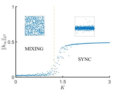
a b

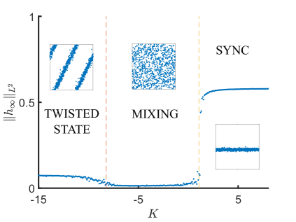
Figure 2: The bifurcation diagrams for the second order KM on ER (a) and SW (b) random graphs. In these experiments, the intrinsic frequences are taken from the normal distributrion with mean $0$ and standard deviation equal to $0.3$. The parameters used for generating ER and SW graphs are $p=0.5$ for the former and $p=0.1$ and $r=0.3$ for the latter. The plot in (a) shows a pitchfork bifurcation at $K_{c}>0$. The bifurcation diagram for the small-world family shows two bifurcations at $K_{c}^{+}>0$ and $K_{c}^{-}<0$. The latter features a spatially heterogeneous pattern bifurcating from mixing, because the eigenfunction of $\boldsymbol{W}$ corresponding to the smallest negative eigenvalue $\mu_{min}$ is not constant (see text for details). The red dashed lines indicate pitchfork bifurcations identified analytically. These values are in good agreement with the results of numerical simulations.

5 Examples

In this section, we apply the theory developed in the previous sections to identify the pitchfork bifurcations in the KM with inertia on Erdős-Rényi (ER) and small-world (SW) graphs. The eigenvalues and eigenfunctions of the integral operator $\boldsymbol{W}$ corresponding to these graphs were computed in our previous work [3]. Below, we will use this information without any further explanations. An interested reader is referred to [3] for more details.

5.1 ER graphs

An ER graph $G(n,p)$ is a graph on $n$ nodes, for which the probability of two given nodes being connected by an edge is equal to $p\in(0,1)$. The edges between distinct pairs of nodes are assigned independently. $G(n,p)$ is a convergent sequence of graphs, whose limit is given by a constant function $W\equiv p$. The largest eigenvalue of $\boldsymbol{W}$ is $\mu_{max}=p$, and the corresponding eigenfunction is constant $V_{max}\equiv 1$ (cf. [3]). Thus, there is a pitchfork bifurcation at

$$K_{c}=\frac{1}{pg_{0}},$$

where $g_{0}$ is defined in (3.23). The bifurcation diagram in Fig. 2 b shows that in the vicinity of $K_{c}$ the order parameter undergoes a sharp transition from very small positive values to the values close to $0.5$. This corresponds to the loss of stability of mixing and the onset of synchronization. Since $V_{max}$ is constant, the unstable mode is spatially homogeneous. With minor modifications the analysis of the pitchfork bifurcation can be extended to sparse Erdős–Rényi graphs [10].

5.2 SW graphs

There are two types of random connections in a SW graph: the short-range and the long-range. The former are assigned with probability $1-p$ and the latter are assigned with probability $p\in(0,1/2)$. The connectivity is defined by another parameter $r\in(0,1/2)$ (see [9] for the exact definition the SW graph sequence used here). SW graphs in [9] are defined as W-random graphs with the limiting graphon

$$W(x,y)=\left\{\begin{array}[]{cc}1-p,&d(x,y)<r,\\ p,&\;\mbox{otherwise}.\end{array}\right.,$$

where $d(x,y)=\min\{|x-y|,1-|x-y|\}$. The eigenvalues and the corresponding eigenfunctions of $\boldsymbol{W}$ for the SW graphs can be found in [3]. In particular, the largest positive eigenvalue $\mu_{max}=2r+p-4rp$ is simple and the corresponding eigenfunction $V_{max}\equiv 1$. This yields a pitchfork bifurcation at $K_{c}^{+}=\left(g_{0}(2r+p-4rp)\right)^{-1}.$

In addition, $\boldsymbol{W}$ has negative eigenvalues. As was explained in Remark 4.1, if the smallest negative eigenvalue $\mu_{min}$ is simple, then there is another bifurcation at $K_{c}^{-}=\left(g_{0}\mu_{min}\right)^{-1}$. The value of $\mu_{min}$ has the following form

$$\mu_{min}=(\pi k^{\ast})^{-1}(1-2p)\sin\left(2\pi k^{\ast}\right)$$

for some integer $k^{\ast}\neq 0$, which is not available analytically in general. The corresponding eigenfunction $V_{min}=e^{2\pi{\mathrm{i}\mkern 1.0mu}k^{\ast}x}$ is not constant anymore. This implies that in contrast to the bifurcation at $K_{c}^{+}$, the steady state bifurcating from mixing at $K^{-}_{c}<0$ is heterogeneous (Fig. 2b). In [4], a bifurcation for a non-constant eigenfunctions and the corresponding twisted state is studied for the classical KM in detail.

Acknowledgements. The authors thank Matthew Mizuhara for providing numerical bifurcation diagrams. This work was supported in part by NSF grant DMS 2009233 (to GSM).

References

- [1] Hayato Chiba, A proof of the Kuramoto conjecture for a bifurcation structure of the infinite-dimensional Kuramoto model, Ergodic Theory Dynam. Systems 35 (2015), no. 3, 762–834.
- [2] , A spectral theory of linear operators on rigged Hilbert spaces under analyticity conditions, Adv. Math. 273 (2015), 324–379.
- [3] Hayato Chiba and Georgi S. Medvedev, The mean field analysis of the Kuramoto model on graphs I. The mean field equation and transition point formulas, Discrete Contin. Dyn. Syst. 39 (2019), no. 1, 131–155.
- [4] , The mean field analysis of the Kuramoto model on graphs II. Asymptotic stability of the incoherent state, center manifold reduction, and bifurcations, Discrete Contin. Dyn. Syst. 39 (2019), no. 7, 3897–3921.
- [5] Helge Dietert, Stability and bifurcation for the Kuramoto model, J. Math. Pures Appl. (9) 105 (2016), no. 4, 451–489.
- [6] R. L. Dobrušin, Vlasov equations, Funktsional. Anal. i Prilozhen. 13 (1979), no. 2, 48–58, 96.
- [7] Dmitry Kaliuzhnyi-Verbovetskyi and Georgi S. Medvedev, The mean field equation for the Kuramoto model on graph sequences with non-Lipschitz limit, SIAM Journal on Mathematical Analysis 50 (2018), no. 3, 2441–2465.
- [8] Y. Kuramoto, Cooperative dynamics of oscillator community, Progress of Theor. Physics Supplement (1984), 223–240.
- [9] Georgi S. Medvedev, Small-world networks of Kuramoto oscillators, Phys. D 266 (2014), 13–22.
- [10] , The continuum limit of the Kuramoto model on sparse random graphs, Commun. Math. Sci. 17 (2019), no. 4, 883–898. MR 4030504
- [11] F. Salam, J. Marsden, and P. Varaiya, Arnold diffusion in the swing equations of a power system, IEEE Transactions on Circuits and Systems 31 (1984), no. 8, 673–688.
- [12] Barry Simon, Basic complex analysis, A Comprehensive Course in Analysis, Part 2A, American Mathematical Society, Providence, RI, 2015.
- [13] Hisa-Aki Tanaka, Maria de Sousa Vieira, Allan J. Lichtenberg, Michael A. Lieberman, and Shin’ichi Oishi, Stability of synchronized states in one-dimensional networks of second order PLLs, Internat. J. Bifur. Chaos Appl. Sci. Engrg. 7 (1997), no. 3, 681–690.
- [14] Hisa-Aki Tanaka, Allan J. Lichtenberg, and Shin’ichi Oishi, Self-synchronization of coupled oscillators with hysteretic responses, Physica D: Nonlinear Phenomena 100 (1997), no. 3, 279 – 300.
- [15] Liudmila Tumash, Simona Olmi, and Eckehard Schőll, Stability and control of power grids with diluted network topology, Chaos: An Interdisciplinary Journal of Nonlinear Science 29 (2019), no. 12, 123105.