The Noonday Argument: Fine-Graining, Indexicals, and the Nature of Copernican Reasoning

Abstract

Typicality arguments attempt to use the Copernican Principle to draw conclusions about the cosmos and presently unknown conscious beings within it. The most notorious is the Doomsday Argument, which purports to constrain humanity’s future from its current lifespan alone. These arguments rest on a likelihood calculation that penalizes models in proportion to the number of distinguishable observers. I argue that such reasoning leads to solipsism, the belief that one is the only being in the world, and is therefore unacceptable. Using variants of the “Sleeping Beauty” thought experiment as a guide, I present a framework for evaluating observations in a large cosmos: Fine Graining with Auxiliary Indexicals (FGAI). FGAI requires the construction of specific models of physical outcomes and observations. Valid typicality arguments then emerge from the combinatorial properties of third-person physical microhypotheses. Indexical (observer-relative) facts do not directly constrain physical theories. Instead they serve to weight different provisional evaluations of credence. These weights define a probabilistic reference class of locations. As indexical knowledge changes, the weights shift. I show that the self-applied Doomsday Argument fails in FGAI, even though it can work for an external observer. I also discuss how FGAI could handle observations in large universes with Boltzmann brains.

I Background

What can we learn from the simple fact that we exist where and when we do? The answer may bear on many profound questions, including the nature and size of the cosmos, the existence and types of extraterrestrial intelligence, and the future of humanity.

Attempts to reason about the cosmos from the fact of our existence have been called anthropic reasoning [e.g., 1, 2]. The anthropic principle argues that our existence is expected even if the events that lead up to it are rare [3]. In its weakest form, it simply asserts that humanity’s existence is probabilistically likely in a large enough universe [4]. The strongest versions of the anthropic principle have an opposite premise at heart [2]: our existence is not a fluke, but somehow necessary in a logical sense [5]. Anthropic reasoning has been extended to include Copernican principles, which emphasize the typicality of our environment. Weak forms point out our evolution was not a special rupture in the laws of physics, but one possible outcome that can be repeated if given enough “trials” in sufficiently many cosmic environments like ours. Strong forms state that conscious beings (“observers”) like ourselves are common.

Anthropic reasoning frequently tries to synthesize the anthropic and Copernican principles: we should regard our circumstances as typical of observers like ourselves. Bostrom [2] has formalized this notion as the Self-Sampling Assumption (SSA). The group of observers considered similar enough to us for Copernican reasoning to be valid is our “reference class”. It may be as wide as all possible sentient beings or as narrow as people exactly identical to your current self. There is no consensus on a single reference class, or indeed whether we might use a multitude [e.g., 6, 7, 2], although the more extreme Copernican formulations apply the universal reference class of all observers. Typicality arguments are often justified in normal experiments to derive conclusions when unusual outcomes are expected given enough “trials”. In fact, some kind of typicality assumption seems necessary to reason about large cosmologies, where thanks to the anthropic principle there will exist observers like ourselves with certainty even in Universes distinct from ours – otherwise observations have no power to constrain the nature of the world [8, 9]. Typicality is commonly invoked in discussions of cosmology as the “principle of mediocrity” [10].

The seemingly reasonable Copernican statement of the SSA has led to controversy, as it can be applied to constrain the cosmological contexts of as-of-yet unobservable intelligences in the Universe. Few applications of the Copernican principle are more contentious than the Doomsday Argument. In its most popular form as presented by Gott [11], we are most likely “typical” humans and therefore are unlikely to be near humanity’s beginning or end [see also 12]. The Bayesian Doomsday Argument, most strongly defended by Leslie [1], has a more robust basis: our birthrank (the number of humans before us) is treated as a uniform random variable drawn from the set of all birthranks of the final human population. A larger human population has more “outcomes”, resulting in a smaller likelihood of “drawing” your specific birthrank and a Bayesian shift favoring a short future for humanity [see also 13, 2]. A generalized non-ranked variant has been brought to bear to evaluate the existence of beings unlike ourselves in some way, as in the Cosmic Doomsday argument [14].

The Doomsday Argument and similar typicality arguments would have profound implications for many fields. For example, in the Search for Extraterrestrial Intelligences [SETI 15] the prevalence of technological societies is critically dependent on the lifespan of societies like our own [e.g., 16, 17, 18]. Doomsday would be an extraordinarily powerful argument against prevalent interstellar travel, much less more exotic possibilities of astronomical-scale “megastructures” [19, 20]. The instantaneous population of a galaxy-spanning society could be $\sim 10^{20}$ [11, 14] while predictions of intergalactic travel and astro-engineering suggest populations greater than $10^{50}$ [21, 22]. Yet the Doomsday Argument applies huge Bayes Factors against the viability of these possibilities or indeed any long future, essentially closing off the entire field of SETI as difficult to futile [11]. Similar Bayesian shifts might drastically cut across theories in other fields, like landscape hypotheses.

This sheer power cannot be stressed enough. These likelihood ratios for broad classes of theories ($>10^{40}$ in some cases!) imply more than mere improbability, they are far more powerful than those resulting from normal scientific observation. If we have any realistic uncertainty in such futures, even the slightest possibility of data being hoaxed or mistaken (say $10^{-9}$) results in epistemic closure. If we discovered a galaxy-spanning society, or if we made calculations implying that the majority of observers in the standard cosmology live in realms where the physical constants are different from ours, then the evidence would force us to conclude that scientists are engaged in a diabolical worldwide conspiracy to fake these data. The SSA even can lead to paradoxes where we gain eerie “retrocausal” influence over the probabilities of past events by prolonging humanity’s lifespan [23].

Given the unrealistic confidence of the Doomsday Argument’s assertions, it is not surprising that there have been many attempts to cut down its power and either tame or refute typicality [e.g., 24, 25, 26, 27, 28, 6, 2, 29, 30]. These include disputing that our self-observation can be compared to a uniformly drawn random sampling [24, 26, 30], arguing for the use of much narrower reference classes [6, 2, 31], or rejecting the use of a single Bayesian credence distribution [32, 29]. The most common attack is the Self-Indication Assumption (SIA): if we really are drawn randomly from the set of possible observers, then any given individual is more likely to exist in a world with a larger population. The SIA demands that we adopt a prior in which the credence placed on a hypothesis is directly proportional to the number of observers in it, which is then cut down by the SSA using our self-observation [24, 25, 28, see also Neal 6 for further discussion]. Yet this prior too posits absurd levels of confidence, not at all like how we actually reason: we do not actually start out assuming a posthuman galactic future is $\gtrsim 10^{20}$ times more likely than one where we go extinct in 2100, and then update to equal credence upon learning we live in 2021. Moreover, the SIA leads to the Presumptuous Philosopher problem: the SIA prior leads us to favor cosmologies where the Universe is large, possibly to a ridiculous degree (say, $\sim 10^{100}$) without ever making any observations [33, 34]. But the Doomsday Argument is a Presumptuous Philosopher problem in spirit too, just in the opposite direction – one develops extreme certainty about far-off locations without ever observing them.

In this paper, I critically examine and deconstruct the Copernican typicality assumptions used in the Doomsday Argument and present a framework for understanding them, Fine Graining with Auxiliary Indexicals (FGAI). I start with an analysis of the self-applied Doomsday Argument and how it can lead to solipsism (Section II). Using the “Sleeping Beauty” thought experiment, I illustrate the disanalogy between these arguments and similar-seeming valid arguments (Section III). I then lay the groundwork for FGAI by showing how fine-graining cosmological theories can account for many of the uses for typicality without making reference to indexical propositions (Section IV). Section V reintroduces indexical credences as weights for physical credence distributions. Finally, I discuss the nature of the Copernican Principle and summarize why the self-applied Doomsday Argument fails in FGAI (Section VI).

Throughout this paper, I use the terms “Small” and “Large” to broadly group theories about unknown observers [as in 1]. In Small theories, the majority of actually existing observers are similar to us and make similar observations of their environment, while Large theories propose additional, numerically dominant populations very dissimilar to us. When specifically talking about the lifespan of a population, a “Short” history is one that is Small while a “Long” history is one that is Large (e.g., $N_{\rm total}\gg 10^{11}$ for human history).

II The Doomsday Argument and its terrible conclusion

The Doomsday Argument is arguably the most far-reaching and contentious of the arguments from typicality. It generates enormous Bayes factors against its Large models, despite relatively plausible (though still very uncertain) routes to Large futures. By comparison, we have no specific theory or forecast implying that inorganic lifeforms [c.f., 6] or observers living under very different physical constants elsewhere in a landscape dominate the observer population by a factor of $\gg 10^{10}$. Cases where we might test typicality of astrophysical environments, like the habitability of planets around the numerically dominant red dwarfs [35], generate relatively tame Bayes factors of $\sim 10\text{--}100$ that seem plausible (a relatively extreme value being $\sim 10^{4}$ for habitable planets in elliptical galaxies from [36, 37]). For this reason, it is worth considering Doomsday as a stringent test of the “Copernican Princple”.

Let us consider how the Doomsday Argument works and the SSA’s role in it.

II.1 Noonday, a parable

A student asked their teacher, how many are yet to be born?

The teacher contemplated, and said: “If the number yet to be born equaled the number already born, then we would be in the center of history. Now, remember the principle of Copernicus: as we are not in the center of the Universe, we must not be in such a special time. We must evaluate the $p$-value of a possible final population as the fraction of people who would be closer to the center of history.

“Given that 109 billion humans have been born so far,” continued the teacher, citing Kaneda and Haub [38], “The number of humans yet to be born is not between 98 and 119 billion with 95% confidence. There may be countless trillions yet to be born, or none at all, but if you truly believe in Copernicus’s wisdom, you must be sure that the number remaining is not 109 billion.”

And so all who spoke of the future from then on minded the teacher’s Noonday Argument.

II.2 Noonday, $x$-day , and the frequentist Doomsday Argument

In its popular frequentist form, the Doomsday Argument asks Wouldn’t it be strange if we happened to live at the very beginning or end of history? It applies whether considering the temporal lifespan of humanity, the number of people ever born, or any other measure $z_{\rm present}$ of how much history has passed so far compared to humanity’s total history measure $z_{\rm total}$. Let $F\equiv z_{\rm present}/z_{\rm total}$ be the fraction of history that has passed, a value between $0$ and $1$. If we regard $F$ as a uniform random variable, the probability of drawing $F$ closer to $0$ or $1$ than a value $f$ is $\overline{p}=\min(2f,1-2f)$. We construct a confidence interval with probability $p\equiv 1-\overline{p}$ by bounding our $F$ to be between $\overline{p}/2$ and $1-\overline{p}/2$: $z_{\rm present}/(1-\overline{p}/2)\leq z_{\rm total}\leq z_{\rm present}/(\overline{p}/2)$ with probability $p$ [11].

This form does not specifically invoke the SSA: $F$ can parametrize measures like lifespan that have nothing to do with “observers” and require no reference class. In fact, it is motivated by an analogy to externally-applied Doomsday arguments, in which the lifespan of a phenomenon is inferred by making an age measurement of a randomly selected member of a population [11]. Unlike the Bayesian Doomsday Argument, it penalizes models where $F=1$ (Section II.3).

The parable of the Noonday Argument demonstrates the weakness of the frequentist Doomsday Argument: it is not the only confidence interval we can draw. The Noonday Argument gives another, one arguably even more motivated by the Copernican notion of us not being in the “center” [c.f., 27]. An infinite or zero future is maximally compatible with the Noonday Argument. But there is no reason to stop with Noonday either. Wouldn’t it be strange if our $f$ happened to be a simple fraction like $1/3$, or some other mathematically significant quantity like $1/e$? Or if we pick a random number from $[0,1]$ with the aid of, say, radioactive decay, surely that cannot predict our future by being unusually close to our $f$?

Doomsday and Noonday are just two members of a broad class of $x$-day Arguments. Given any $x$ in the range $[0,1]$, the $x$-day Argument is the observation that it is extremely unlikely that a randomly drawn $F$ will just happen to lie very near $x$. To handle edge cases, we regard the interval $[0,1]$ as cyclic, just like the frequentist Doomsday Arugment. The $x$-day confidence interval with confidence level $p=1-\overline{p}$ is $[z_{\rm present}/(x+(1-\overline{p}/2)),z_{\rm present}/(x+\overline{p}/2)]$ if $x\leq\overline{p}/2$, $[z_{\rm present},z_{\rm present}/(x+\overline{p}/2)]\cup[z_{\rm present}/(x-\overline{p}/2),\infty)$ if $\overline{p}/2<x<1-\overline{p}/2$, or $[z_{\rm present}/(x-\overline{p}/2),z_{\rm present}/(x+(1-\overline{p}/2))]$ if $1-\overline{p}/2\leq x$. The Doomsday Argument is simply the $0$-day Argument and the $1$-day Argument, whereas the Noonday Argument is the ½-day Argument.

By construction, all frequentist $x$-day Arguments are equally valid frequentist statements if $z_{\rm present}$ truly is a random variate with a uniform distribution. Any notion that being near the beginning, the end, or the center is “strange” is just a subjective impression, one that has no bearing on these constructions. The confidence intervals are disjoint but their union covers the entire range of possibilities, with an equal density for any $p$ covering any $z_{\rm present}$ value [27]. In fact, one can generalize the $x$-day argument to all kinds of confidence intervals – there is no reason we could not construct one for any measurement by “excluding” a small range of values closest to a measurement.

The Noonday Argument demonstrates that not every plausible-sounding Copernican argument is useful, even when technically correct. A proper Doomsday-style Argument therefore requires something more than the probability of being near a “special” time. When dealing with continuously varying parameters and a continuous likelihood function, any specific parameter value can be excluded simply by changing the bounds of integration. Confidence intervals merely summarize the effects of likelihood – which is small for Large models, as reflected by the relative compactness of the 0/1-day intervals.

II.3 Bayesian Doomsday and Bayesian Noonday

Bayesian statistics is a model of how our levels of belief, or credences, are treated as probabilities conditionalized by observations. We have a set of some models we wish to constrain, and we start with some prior credence distribution over them. The choice of prior is subjective, but a useful prior when considering a single discrete parameter $\lambda$ of unknown scale is the flat log prior: $P^{\rm prior}(\lambda)\propto 1/\lambda$. This credence distribution is then modified in proportion to the likelihood ${\cal L}(\bm{\lambda_{i}}|D)$ of the observed data $D$ in each model $\bm{\lambda_{i}}$, which is simply the probability $P(D|\bm{\lambda_{i}})$ in that model that we observe $y$. Bayes’ theorem then gives us a posterior credence distribution, with an updated credence for the model parameters $\bm{\lambda_{i}}$:

$$P^{\rm pos}(\bm{\lambda_{i}}|D)=\displaystyle\frac{P^{\rm prior}(\bm{\lambda_{i}}){\cal L}(\bm{\lambda}|D)}{\sum_{\bm{\lambda_{j}}\in\Lambda}P^{\rm prior}(\bm{\lambda_{j}}){\cal L}(\bm{\lambda_{j}}|D)},$$ (1)

where $\Lambda$ is the set of possible $\bm{\lambda}$.

Bayesian probability provides a more robust basis for the Doomsday Argument, and an understanding of how it supposedly works. In the Bayesian Doomsday argument, the parameter we seek to constrain is the final total population of humanity and its inheritors, $N_{\rm total}$, using birthranks as the observable. The key assumption is to apply the SSA with all of humanity and its inheritors as our reference class. If we view ourselves as randomly selected, our birth rank $N_{\rm past}$ is drawn from a uniform distribution over $[0,N_{\rm total}-1]$, with a likelihood of $0$ if $N_{\rm total}<N_{\rm past}$ and $1/N_{\rm total}$ if $N_{\rm total}\geq N_{\rm past}$. Starting from the uninformative flat prior $P^{\rm prior}(N_{\rm total})\propto 1/N_{\rm total}$, applying Bayes’ theorem then results in the following posterior:

$$P^{\rm pos}(N_{\rm total})\propto\left\{\begin{array}[]{ll}0&(N_{\rm total}<N_{\rm past})\\ 1/N_{\rm total}^{2}&(N_{\rm total}\geq N_{\rm past}).\end{array}\right..$$ (2)

The posterior in equation 2 is strongly biased against Large models, with $P^{\rm pos}(N_{\rm total}\geq N)\approx N_{\rm past}/N$.

Birthrank is indeed the most natural basis for the Doomsday Argument, and thus the Argument depends on observers (or observer-moments). Birthrank is necessarily distributed uniformly. In contrast, age measurements are likely to be biased – in an exponentially growing population, for example, most measurements are made by people living near the end. This emphasizes the role of the SSA.

The parable’s trick of excluding $N_{\rm total}$ values near $2N_{\rm past}$ is irrelevant here. Bayesian statistics does define credible intervals containing a fraction $p$ of posterior credence and we could draw Noonday-like intervals that include Large models but exclude a narrow range of Small models. But this is simply sleight-of-hand, using well-chosen integration bounds to hide the fundamental issue that $P^{\rm pos}(N_{\rm total}\gg N_{\rm past})\ll 1$.

But could there be a deeper $x$-day Argument beyond simply choosing different credible intervals? Perhaps not in our world, but we can construct a thought experiment where there is one. Define an $x$-ranking as $N_{x}=N_{\rm past}-xN_{\rm total}$; allowed values are in the range of $[-xN_{\rm total},(1-x)N_{\rm total}]$. If through some quirk of physics we only knew our $N_{x}$ , we would treat $N_{x}$ as a uniform random variable, calculate likelihoods proportional to $1/N_{\rm total}$ and derive a posterior of $1/N_{\rm total}^{2}$ for allowed values of $N_{\rm total}$ ($N_{\rm total}\geq-N_{x}/x~{}\textrm{and}~{}N_{x}<0~{}\textrm{or}~{}N_{\rm total}\geq N_{x}/(1-x)~{}\textrm{and}~{}N_{x}>0$). Thus all Bayesian $x$-day Arguments rule out Large worlds, including the Bayesian Noonday Argument, even though the parable’s Noonday Argument implies we should be perfectly fine with an infinite history. This is true even if $x$ is not “special” at all: most of the $x$-day Arguments are perfectly consistent with a location in the beginning, the middle, or the end of history – anything is better than having $f\approx x$, even if the maximum likelihood is for a “special” location. For example, the Bayesian Doomsday Argument, which uses our $0$-ranking, predicts a maximum likelihood for us being at the very end of history. The oddity is also clear if we knew a cyclic Noonday rank $N_{1/2}^{\prime}$ that wraps from the last to the first human: the most likely $N_{\rm total}$ value would be $N_{1/2}^{\prime}+1$, a seemingly anti-Copernican conclusion favoring us being adjacent to the center of history.

The Bayesian $x$-day Arguments provide insight into the heart of the Bayesian Doomsday Argument, which has nothing to do with the beginning, middle, or end of history being “special”. What powers all of these arguments is the SSA applied with a broad reference class: the $1/N_{\rm total}$ factor in the likelihood. According to these SSA-based arguments, the reason Large worlds are unlikely is because measuring any particular value of $N_{x}$ whatsoever is more unlikely as $N_{\rm total}$ increases. This is a generic property when one actually is randomly drawing from a population; it does not even depend on numerical rankings at all. Ultimately, the result follows from the Bayesian Occam’s Razor effect, in which Bayesian probability punishes hypotheses with many possible outcomes [39].

II.4 The Presumptuous Solipsist

The SSA is doing all of the work in the $x$-day Arguments, but nothing restricts its applications solely to birth rankings or $N_{x}$ in general. In fact, the unrestricted SSA argues against Large models of all kinds. It can be used to derive “constraints” on all kinds of intelligences. One example is the Cosmic Doomsday argument against the existence of interstellar societies, solely by virtue of their large populations regardless of any birthrank [14]. If thoroughly applied, however, it would lead to shockingly strong evidence on a variety of matters, from cosmology to astrobiology to psychology [as noted by 6, 40].

The existence of non-human observers is widely debated. Several theories of physics predict a universe with infinite extent (in space, time, or otherwise), including the open and flat universes of conventional cosmology, eternal inflation, cyclic cosmology, and the many-world interpretation of quantum mechanics. In each of these models, every possible observer is almost surely realized, with a nearly endless panoply of Earths at least slightly different from ours. But according to the unrestricted SSA, the probability that a randomly selected observer would find themselves in this version of Earth might as well be zero in a sufficiently big universe. The unrestricted SSA also rules out the existence that most of the Universe’s sentient population is not humanlike in some way, like having a non-carbon based biology or living in the sea. In fact it obliterates the case for SETI even without the Doomsday Argument, for if many aliens existed in the Universe, what would the probability be of being born a human instead any of the panoply of extraterrestrial species that are out there? It also makes short work of the question of the question of animal consciousness. Isn’t it strange that, of all the creatures on the Earth, you happen to be human? The SSA would be a strong argument against the typical mammal or bird being a conscious observer, to say nothing of the trillions of other animals.

Unrestrained application of the SSA leads to a far more radical, and ominous conclusion, however. Why not apply the SSA to other humans? We can do this even if we restrict our reference class to humanity and remain agnostic about multiverses, aliens, and animal consciousness. Solipsism, the idea that one is the only conscious being in existence and everything else is an illusion, is an age-old speculation. Obviously, most people do not favor solipsism a priori, but it cannot actually be disproved, only ignored as untenable.

What happens when we apply the SSA to our sliver of solipsistic doubts? Let $\epsilon$ be the credence you assign to all solipsistic ideas that are constrained by SSA. To be sure, we usually do not grant much credence to solipsism, so perhaps $\sim 10^{-9}$ is a reasonable value. But if one is not unduly prejudiced against solipsism, $\epsilon$ cannot be zero. If one woke up to find one’s perceptions of the Universe melting away, leaving one as an isolated Boltzmann brain in a tiny collapsing cosmos, for example, surely one would want to at least be able to entertain that idea (see Section V.10). The remaining credence, $1-\epsilon$ will be assigned to the idea that other people are real. What are the odds that you are you, according to the SSA? The principle assigns a likelihood of $\leq 1/10^{11}$ for a realist worldview; only the normalization factor in Bayes’ theorem preserves its viability. But the SSA indicates that, according to solipsism, the likelihood that an observer has your data instead of the “data” of one of the hallucinatory “observers” you are imagining is 1. From the point of view of solipsism, the premise that other people actually exist is a Large model. Applying Bayes’ theorem, the credence you should now assign to it is $P_{\rm solip}\geq\epsilon/[1/N_{\rm past}+\epsilon(1-1/N_{\rm past})]$:

$$P_{\rm solip} \gtrsim\left\{\begin{array}[]{ll}1-1/(\epsilon N_{\rm past})&(\epsilon N_{\rm past}\gg 1)\\ \epsilon N_{\rm past}&(\epsilon N_{\rm past}\lesssim 1)\end{array}\right..$$ (5)

If your prior willingness to entertain solipsism was above $\sim 10^{-11}$, the SSA magnifies it into a virtual certainty.

Actually, the situation is much worse: Bostrom [2] further proposes a Strong Self-Sampling Assumption (SSSA), wherein individual conscious experiences are the fundamental unit of observations. What are the odds that you happen to make this observation at this point of your life instead of any other? Suppose it takes 100 seconds to fully make the observation that one exists in this moment, presumably a generous estimate. Given a mean human life expectancy over history of ten years [38], the SSSA increases $N_{\rm past}$ by a factor of $\sim 3$ million. Your credence in extreme solipsism, where only your current observer-moment exists, should be amplified by a factor $\sim 3\times 10^{17}$, and more if one believes there is good evidence for an interstellar future, animal consciousness, alien intelligences, or the existence of a multiverse. Unless one is unduly prejudiced against it – invoking the absurdly small prior probabilities that are the problem in the SIA – the principle behind the Doomsday Argument impels one into believing nobody else in existence is conscious, not even your past and future selves. The SSSA does allow there to be multiple copies of you, exactly identical to yourself, since you have no way of telling which of these selves you are, but that is hardly any consolation.

One might object that “me, now” is a superficial class, that everyone in the real world is just as unique and unrepresentative, so there is no surprise that you are you instead of everything else. This is invalid according to unrestricted Copernican reasoning. You are forced to grapple with the fundamental problem that your solipsistic model has only one possible “outcome” but realist models have many because there really do exist many different people – in the same way that drawing a royal flush from a stack of cards on the first try is very strong evidence it is rigged even if every possible draw is equally unlikely with a randomly shuffled deck. Nor can one argue a distinction in that all currently living people are equally typical as distinct individuals, whereas a Large future would have us living in an atypically “special” time in a Large future. The $x$-day Arguments show that there exists an $N_{x}$ that is small for each individual in any population. We have no reason to limit Doomsday to birthrank instead of any measure of similarity between people – to do so is ignoring data.

Later sections will provide a way out of solipsism even if one accepts the SSA (Section V.2). This is to fine-grain the solipsism hypothesis by making distinctions about what the sole observer hallucinates, or which of all humans is the “real” one. The distinctions between specific observers are thus important and cannot be ignored. In the context of the Doomsday Argument, we can ask what is the likelihood that the sole solipsist observer imagines themself to have a birthrank of $10^{11}$ instead of $1$ or $10^{50}$. Indeed, Section IV argues that fine-graining is an important part of understanding the role of typicality. As we will see, using fine-grained models can impose constraints that prevent its use in Doomsday Arguments.

II.5 The anti-Copernican conclusion of the maximal Copernican Principle

The Copernican Principle is inherently unstable when adopted uncritically. Even a small perturbation to one’s initial prior, a sliver of doubt about there really being 109 billion people born so far, is magnified to the point where it can completely dominate one’s views about the existence of other beings. This in turn leads to epistemic instability, as everything one has learned from the external world is thrown into doubt. Although the SSA started out as a way of formalizing the Copernican Principle, it has led to what may be considered an anti-Copernican conclusion in spirit. Weaker Copernican principles suggest that you consider yourself one of many possible minds, not considering yourself favored, just as the Earth is one of many planets and not the pivot of the Universe. But this strong formulation suggests that you are the only kind of mind, unique in all of existence. Instead of a panoply of intelligences, we get at most an endless procession of copies of you and no one else. Like the anthropic principle, the most extreme versions of the Copernican principle presumptuously tell you that you are fundamental.

III Deconstructing typicality

III.1 Why is typicality invoked at all?

Typicality, the principle behind the SSA, has been invoked to explain how we can conclude anything at all in a large Universe. Since the Universe appears to be infinite, all possible observations with nonzero probability will almost surely be made by some observers somewhere in the cosmos by the anthropic principle. That is, the mere fact that there exists an observer who makes some observation has likelihood $1$ in every cosmology where it is possible. Furthermore, a wide range of observations is possible in any given world model. Quantum theories grant small but nonzero probabilities for measurements that diverge wildly from the expected value: that a photometer will detect no photons if it is pointed at the Sun, for example, or that every uranium nucleus in the Earth will spontaneously decay within the next ten seconds. Most extreme are Boltzmann brains: any possible observer (for a set of physical laws) with any possible memory can be generated wherever there is a thermal bath. Thus we expect there exist observers who make any possible observation in infinite cosmologies that can sustain cognition. Without an additional principle to evaluate likelihoods, no evidence can ever favor one theory over another and science is impossible [8, 9, 32, 2].

The common solution has been to include indexical information in our distributions. Indexicals are statements relating your first-person experience to the outside world. They are not meaningful for a third-person observer standing outside the world and perceiving its entire physical content and structure. The SSA, and the SIA in reply, attempt to harness indexicals to learn things about the world: they convert the first-person statement into a probabilistic objective statement about the world, by treating you as a “typical” observer. Frequently, the physical distinctions between observers are left unspecified, as if they are intrinsically identical and only their environments are different.

When we make an observation, we do at least learn that we are an observer with data $D$, which is indexical information. The idea of these arguments, then, is to construct a single joint distribution for physical theories about the third-person nature of the cosmos and indexical theories about which observer we are. Often this is implicit – rather than having specified theories about which observer we are, indexical information is evaluated with an indexical likelihood, the fraction of observers in our reference class with data $D$. While all possible observations are consistent with a theory in an infinite Universe, most observations will be clustered around a typical value that indicates the true cosmology [2]. Thus the indexical likelihoods result in us favoring models that predict most observers have data similar to ours over those where our observations are a fluke.

Typicality is usually fine for most actual cosmological observations, but it yields problematic conclusions when attempting to choose between theories with different population sizes. These problems will motivate the development of Fine-Graining with Attached Indexicals (FGAI) approach to typicality over the next three sections.

III.2 Sleeping Beauty as three different thought experiments

The core of the Doomsday Argument can be modeled with a thought experiment known as the Sleeping Beauty problem [45]. In this thought experiment, all participating observers are treated as indistinguishable. Imagine that you are participating in experiment in which you wake up in a room for some number of days. Each day your memory of any previous days has been wiped, so you have no sense of which day it is. Now, suppose you knew that the experiment was either Short, lasting for just Monday, or Long, lasting for Monday and Tuesday. In the original formulation of the thought experiment (SB-O), the experimenters flip a coin, running the Short version if it came up Heads and the Long version if it came up Tails [45]. You wake up in the room, not knowing how the coin landed, ignorant of whether you are in a Short run or a Long run. What probability should you assign to the possibility that the coin landed heads and the run is Short, $1/2$ or $1/3$? An intuitive answer might be that you have absolutely no basis to choose between Short and Long because the coin is fair, and that you should have an uninformative prior assigning weight $1/2$ to each possibility. However, the SIA implies that the probability should be $1/3$, because each possible day in each outcome is equally plausible as your current day. More awakenings happen in the Long run, so you’d be more likely to be among them on this day.

If you then learn that it is Monday, the SSA would increase your credence in the Short run. For a prior probability of $1/3$, you would come to believe there is $1/2$ probability you are in the Short run. Applied to the uninformative prior, your credence would instead be $2/3$. The thought experiment is directly analogous to the Doomsday Argument; one either starts with a bias against Short runs (with the SIA) or ends with a bias against Long runs (without the SIA).

The conventional Sleeping Beauty thought experiment has been used to examine the SSA and competing principles [6], but we have to be careful about drawing analogies to our own predicament. We especially must be clear about what probability actually represents, whether it is solely Bayesian and subjective or frequentist and objective. The following versions of the experiment clarify this distinction (see Figure 1):

• (SB-A) You know that the experiments proceed with a Short run followed by a Long run of the experiment, and you are participating in both. Each day, you wake up with an identical psychological state. Today you wake up in the room. With what probability is today one the day you awaken during the Short run?

• (SB-B) The experimenters have decided, through some unknown deterministic process, to run only either the Short or the Long version of the experiment. You have absolutely no idea which one they have decided upon. Each day, you wake up with an identical psychological state. Today you wake up in the room. What credence should you assign to the belief that the experimenters have chosen to do the Short run?

• (SB-C) The experimenters have decided, through some unknown deterministic process, to run only either the Short or a variant of the Long version of the experiment. In the modified Long experiment, they run the experiment on both Monday and Tuesday, but only wake you on one of the two, chosen by another unknown deterministic process. Today you wake up in the room. What credence should you assign to the belief that the experimenters have chosen to do the Short run? If you learn it is Monday, what credence should you then calculate for the Short run?

When we treat indexical facts on the same footing as physical propositions, we are tempted to make analogies between SB-A and SB-B or between SB-C and SB-B. In each case, only one in three of the possible outcomes is in the Short experiment, and only one of the two possible Long experiment awakenings occur on a Monday. Yet these analogies are deeply flawed. Both SB-A and SB-C have obvious uninformative priors yielding the same result with or without the SIA, but they point to different resolutions of the Sleeping Beauty problem: $1/3$ for SB-A and $1/2$ for SB-C.

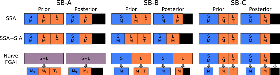
Figure 1: Illustration of how different methods of treating indexicals affect Bayesian credences about Short (S) and Long (L) runs in SB-A, SB-B, and SB-C, before and after learning it is Monday (M) instead of Tuesday (T). The physical theory has already been determined in SB-A, while the observer position in each possible physical theory is determined in SB-C. Ruled out hypotheses are colored in black and do not count towards the normalization. The SSA, with or without the SIA, leads to presumptuous conclusions in SB-B. In naive FGAI, the indexical and physical distributions are not mixed. Instead, there is an overarching physical distribution, and each model has an associated indexical probability distribution (indicated by the arrows).

SB-A and SB-B posit an indexical uncertainty mapping your current first-person experience to one of the identical days. SB-A has this as the only uncertainty, with all relevant objective facts of the world known with complete certainty. Thus, the combined SIA and SSA amount to simply counting days and grouping them; they will give you the right answers most of the time. Because only an indexical is at stake, there can be no Presumptuous Philosopher problem in SB-A – you are already absolutely certain of the “cosmology”. But although it has been reduced to triviality in SB-A, there is actually a second set of credences for the third-person physical facts of this world: our 100% credence in this cosmology, with both a Short and Long run.

In both SB-B and SB-C, you are in a state of total uncertainty about the objective state of the world itself. A Bayesian probability distribution about whether you are in the Short or Long versions has no relation to any objective fact about the matter. The objective frequentist probability that you are in the Short run with SB-B is neither $1/2$ nor $1/3$ – it is either $0$ or $1$. Instead the Bayesian prior is solely an internal one, used by you to weigh the relative merits of different theories of the cosmology of the experiment. Thus, it makes no sense to start out implicitly biased against the Short run, so the probability $1/2$ is more appropriate for a Bayesian distribution. For all you know, the experimentalists are anti-Long run extremists. Minor evidence for that – like finding an anti-Long screed crumpled in the trash can written by a junior associate experimenter – should result in the prior slightly favoring the Short run, which is not possible if we adopt a $1/3$ prior credence in the Short theory.

Attempts to make analogies between situations like SB-A and those like SB-B lead to ambiguous conclusions. Some thought experiments attempt to motivate the Doomsday Argument by making analogies with SB-A-like scenarios – clearly we should believe we are in the more “typical” Long population in that case (e.g., Leslie 1’s “emerald” thought experiment). Yet, arguably this instead justifies the use of the SIA – in SB-A, one is more likely to exist in the Large context of the Long experiment, so we should be predisposed to favor a Large model. But in SB-A-like thought experiments, the physical world model is completely specified and there is no doubt about whether the Large population exists. This same distinction breaks the analogy between these thought experiments and the Doomsday Argument. SB-B posits that you are not just trying to figure out where you are in the world, but the nature of the world in the first place.

We can also contrast SB-B with SB-C, which is more like a typical experiment in that the Large theory has more outcomes but the same number of observers. In SB-C, there are actually two Long hypotheses that split the original $1/2$ credence: one where you awaken on Monday only and one where you awaken on Tuesday only. The big difference between SB-B and SB-C is that there are two possible physical outcomes in SB-C’s Long variant, but only one in SB-B’s – the observations made by all observers in SB-B are determined by whether Short or Long is chosen. Only the limited indexical information available to SB-B’s participant makes it seem like there are two outcomes. This indexical dependence is not present in SB-C, just as there is no physical distinction in SB-A. In SB-C, learning “it is Monday” should result in a changed credence, because learning the physical fact that “a participant awakened on Monday” is not a determined outcome in the SB-C Long theory. This is not a Presumptuous argument because it involves a scientific observation that directly follows from the theory, not a philosophical assumption about typicality. But in SB-B, finding out it’s Monday is consistent with both a Short and Long run, and the likelihood of either given that simple physical fact on its own is $1$, suggesting we should not simply just favor the Short run.

SB-C does not accurately model $x$-day or any of the solipsistic arguments either, where the number of observers itself is at stake. This is illustrated by considering a thought experiment where we try to determine if fish are conscious, supposing that they outnumber humans by a hundred to one. Our theories clearly should be of the form i.) all eight billion humans are conscious but zero fish are, or ii.) all eight billion humans plus the eight hundred billion fish are conscious, possibly with intermediate theories where only some fish are conscious. But the equivalent of SB-C would require the fish-consciousness hypothesis to be ii.) only eighty million humans plus 7.92 billion fish are conscious, an absurdity. It would be absurd even if we didn’t know the world’s population: there is no physical mechanism by which the existence of conscious fish somehow prevents conscious humans from existing. The same disanalogy with SB-C applies to arguments about exotic extraterrestrial intelligences, interstellar futures, and multiverses.

III.3 Separating indexical and physical facts

Simple Bayesian updating does give reasonable results in SB-A and SB-C, where only indexical or only physical propositions are being considered. This suggests that any theory of typicality should reduce to Bayesian updating under these circumstances. But Presumptuous Philosopher-like problems arise in SB-B whether we adopt the SSA alone or the SSA with the SIA. This suggests that it is the mixing of physical and indexical facts into one joint distribution that leads to trouble.

The reason we cannot mix indexical and physical propositions could be because they are fundamentally different. Indexicals are like statements about coordinate systems. We are free to set the origin wherever we want as long as we are consistent, but that freedom does not fundamentally change the way the Universe objectively works. It follows that purely indexical facts cannot directly constrain purely physical world models. The paradoxes are a result of trying to force indexical data into working like physical data.

Since Bayesian updating does work in SB-A and SB-C, we can suppose there are in fact two types of credence distributions, physical and indexical. In FGAI there is an overarching physical distribution describing our credences in physical world models. Attached to each physical hypothesis, there is also an indexical distribution (Figure 1). Each indexical distribution is updated in response to indexical information [c.f., 32]. The physical distribution is insulated from changes in the indexical distribution. Within the context of a particular world-model, one may apply typicality assumptions like the SSA/SIA to the indexical assumption. The separation between physical and indexical distributions protects world models from the extremely small likelihoods of both the SSA and the SIA.

In the Sleeping Beauty thought experiment, when the experimenter announces it is the first day of the experiment, you learn both an physical fact (“a participant wakes up on Monday”) and an indexical fact (“I’m the me waking on Monday”). The physical fact is consistent with both a Short and Long run in all variants of the thought experiment, so the physical prior is unchanged. In SB-B, the indexical fact leaves the Short hypothesis indexical distribution unchanged, but it changes the indexical distribution for the Long theory. FGAI confines the effects of indexical information. In SB-B, the physical prior remains unchanged, and remains at $1/2$ even after learning it is Monday. So the prior probability of a Short run in Sleeping Beauty can be either $1/2$ or $1/3$ [c.f., 46]: it is $1/2$ in the physical model distribution used in SB-B and SB-C and $1/3$ in the indexical distribution used in SB-A.

III.4 The frequentist limit and microhypotheses

Nonetheless, the frequentist $1/3$ probability does in a way slip back in if the experiment is modified to more closely match frequentist assumptions. Consider:

• (SB-Bⁿ) You know for certain that the experiment is being run for $n$ times where $n\gg 1$. Whether a given run is Short or Long is determined through some deterministic but pseudo-random process, such that any possible sequence of Shorts and Longs is equally credible from your point of view. Each day, you wake up with an identical psychological state. Today you wake up in the room. What credence should you assign to the belief that today is happening during a Short run?

Now there is a large number of competing physical hypotheses, $2^{n}$ in total, one for each possible sequence of Shorts and Longs. As before, each of those hypotheses has an attached indexical distribution (Figure 2). From a practical point of view, however, in most of these hypotheses about half of the runs are Short and half are Long. Although the physical hypotheses may differ in detail, the statistical properties of the great majority are similar. Hence, one becomes nearly certain of a roughly even proportion between Short and Long runs simply through combinatorics. Furthermore, this statistical similarity translates to the indexical distributions: in most indexical distributions, $\sim 1/3$ of the awakenings happen in the Short run. As $n$ tends to infinity, the rare outliers with unbalanced Short/Long runs become insignificant, and the physical distribution becomes trivial when viewed from a coarse-grained perspective; only the indexical distributions remain unconstrained. The probability you would most care about is then $1/3$.

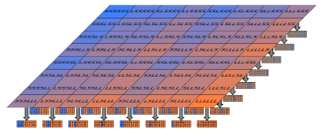
Figure 2: If the Sleeping Beauty experiment is run many times, with each possible sequence of Long and Short a priori equally likely, a vast number of microhypotheses about the sequence of Short and Long is generated. Shown here are the 64 microhypotheses when there are $n=6$ runs. Attached to every single one of these fine models is an indexical distribution.

SB-Bⁿ, where most of the individual sequences are statistically similar, calls to mind statistical mechanics, where a vast number of physical microstates are grouped into a small number of distinguishable macrostates. By analogy, I call each possible detailed world model a microhypothesis, which are then grouped into macrotheories defined by statistical properties.

IV Replacing typicality

IV.1 The fine-grained approach to typicality

How are we to make inferences in a large universe, then, without directly mixing indexicals into the credence distribution? I propose that most of the work performed by typicality can instead be performed by fine-graining. Fine-graining of physical theories is the first principle of FGAI.

The common practice is to treat observers in a fairly large reference class as interchangeable when discussing their observations, but this is merely a convenience. In fact, we can make fine distinctions between observers – between Earth and an inhabited planet in Hubble volume # 239,921, for example, or between me and you, or even between you in 2021 and you in 2020. Macrotheories often cannot predict exactly which specific observer measures a particular datum. Thus, every theory is resolved into myriads of microhypotheses, each of which does make these predictions. Because the distinctions between these observers are physical, statements about a specific observer making a particular measurement are evaluated as purely physical propositions, without invoking indexicals. Some microhypotheses will be consistent with the data, others will not be. The resulting credences in the macrotheories are entirely determined by summing the posterior weight over all microhypotheses, in many cases through simple counting arguments. Typicality then follows from the likelihood values of the microhypotheses – as it indeed does in conventional probability, where specific “special” events like getting a royal flush from a randomly shuffled deck are no more rare than specific mundane outcomes [47]. Thus, in most cases, there is no need to invoke any separate Copernican principle, because it is a demonstrable consequence of our theories.

The other main precept of FGAI is that purely indexical facts do not directly constrain third-person propositions about the physical world, rather modifying indexical distributions attached to each world model. Observations must be treated as physical third-person events when constraining the physical distribution. Statements like “I picked ball 3 out of the urn” or “I am the 109 billionth human” must be recast into third-person statements like “Brian Lacki picked ball 3 out of the urn” or “Mary the Probability Scientist is the 109 billionth human”. Each microhypothesis requires an observation model, a list of possible observations that each observer may make. Observation models necessarily impose physical constraints on which observations can be made by whom, forbidding impossible observations like “Hypatia of Alexandria observed that her peer was Cyborg 550-319447 of Gliese 710” from being considered as possible outcomes.

The fine-graining is most straightforward when every microhypothesis predicts that all physically indistinguishable experiments lead to the same outcome. This follows when we expect conditionalization to entirely restrict possible observations. For example, the Milky Way could be the product of an indeterministic quantum fluctuation, but copies of our Earth with its data (e.g., photographs of the Milky Way from inside) do not appear in elliptical galaxies except through inconceivably contrived series of coincidences. More difficult are purely indeterministic cases, when any specific observer can observe any outcome, which is true for most quantum experiments. I will argue that even then we can form microhypotheses by assuming the existence of an appropriate coordinate system (Section IV.5).

A more serious difficulty is what to do when different plausible indexical hypotheses would lead to different likelihood evaluations for microhypotheses. That is, we may not know enough about where we are to determine whether a microhypothesis predicts an observation or not. In this section, I will adopt the perspective that I call Naive FGAI: we adopt the maximum possible likelihood over all observers we could be, as in the treatment of SB-B in section III.3, because we have no basis for accepting any further conclusion.

IV.2 Naive FGAI

FGAI constructs the physical probability distributions using the Hierarchical Bayes framework, dividing theories into finer hypotheses about internal parameters, possibly with intermediate levels. Suppose we have $M$ macrotheories $\tau_{1}$, $\tau_{2}$, … $\tau_{M}$. Each macrotheory $\tau_{k}$ has $m_{k}$ microhypotheses $\mu_{k,1}$, $\mu_{k,2}$, …, $\mu_{k,m_{k}}$. Each microhypothesis inherits some portion of its parent macrotheory’s credence or weight. Sometimes, when the microhypotheses correspond to exact configurations resulting from a known probabilistic (e.g., flips of an unfair coin), then the prior credence in each $P^{\rm prior}_{k,j}$ can be calculated by scaling the macrotheory’s total prior probability accordingly. In other cases, we have no reason to favor one microhypothesis over another, and by the Principle of Indifference, we assign each microhypothesis in a macrotheory equal prior probability: $P^{\rm prior}_{k,j}=P^{\rm prior}_{k}/m_{k}$. Some macrotheories are instead naturally split into mesohypotheses describing intermediate-level parameters, which in turn are fine-grained further into microhypotheses. Mesohypotheses are natural when different values of these intermediate-level parameters result in differing numbers of outcomes – like if a first coin flip determines the number of further coin flips whose results are reported. Finally, in each $\mu_{k,j}$, we might be found at any of a number of locations. More properly, as observers we follow trajectories through time, following a sequence of observations at particular locations, as we change in response to new data [c.f., 46]. The set $O_{k,j}(D)$ is the set of possible observer-trajectories we could be following allowed by the microhypothesis $\mu_{k,j}$ and the data $D$. The set $O_{k,j}$ describes our reference class if $\mu_{k,j}$ is true.

In Naive FGAI, prior credences $P^{\rm prior}_{k,j}$ in $\mu_{k,j}$ are updated by data $D$ according to:

$$P^{\rm pos}_{k,j}=\frac{\displaystyle P^{\rm prior}_{k,j}\times\max_{i\in O_{k,j}(D)}{\cal L}(\mu_{k,j}|o@i\to D)}{\displaystyle\sum_{x=1}^{M}\sum_{y=1}^{m_{x}}P^{\rm prior}_{x,y}\times\max_{z\in O_{x,y}(D)}{\cal L}(\mu_{x,y}|o@z\to D)},$$ (6)

where ${\cal L}(\mu_{k,j}|o@i\to D)$ is the likelihood of $\mu_{k,j}$ if the observer ($o$) located at position $i$ in $O_{k,j}(D)$ observes data $D$. Of course if the likelihoods are equal for all observers in the reference class $O_{k,j}(D)$, equation 6 reduces to Bayes’ formula. The posterior credences in the macrotheories can be found simply as:

$$P^{\rm pos}_{k}=\sum_{j=1}^{m_{k}}P^{\rm pos}_{k,j}.$$ (7)

Naive FGAI is sufficient to account for many cases where typicality is invoked. Paradoxes arise when the number of observers itself is in question, as in Doomsday, requiring a more sophisticated treatment (Section V).

IV.3 A simple urn experiment

In some cases, microhypotheses and observations models are nearly trivial. Consider the following urn problem: you are drawing a ball from an urn placed before you that contains a well-mixed collection of balls, numbered sequentially starting from $1$. You know the urn contains either one ball (theory A) or ten (theory B), and start with equal credence in each theory. How does drawing a ball and observing its number constrain these theories? Both theory A and theory B have microhypotheses of the form “The urn contains $N$ balls and ball $j$ is drawn at the time of experiment”. In theory A, there is only one microhypothesis, which inherits the full 50% of Theory A’s prior weight. Theory B has 10 microhypotheses, one for each possible draw and each of equal credence, so its microhypotheses start with 5% credence each. Each microhypotheses about drawing ball $j$ has an observation model containing the proposition that you observe exactly ball $j$ – this observation is a physical event, since you are a physical being.

Then the likelihoods of an observed draw is either $1$ (if the ball drawn is that predicted in the microhypothesis) or $0$ (if the ball is not the predicted one). If we draw ball $3$, for example, the credence in all hypotheses except Theory B’s “Ball 3 is drawn” microhypothesis is zero. Then the remaining microhypothesis has 100% credence, and Theory B has 100% credence as well. If instead ball $1$ is drawn, Theory A’s sole microhypothesis and one of Theory B’s microhypotheses survive unscathed, while the other nine microhypotheses of Theory B are completely suppressed. That is, 100% of Theory A’s credence survives, while only 10% of Theory B’s credence remains; therefore, post-observation, the credence in Theory A is $10/11$ and the credence in Theory B is $1/11$. This, of course, matches the usual expectation for the thought experiment.

But what if instead you and 99 other attendees at a cosmology conference were drawing from the urn with replacement and you were prevented from telling each other your results? If we regard all one hundred participants as exactly identical observers, the only distinct microhypotheses seem to be the frequency distribution of each ball $j$ being drawn. Then naive FGAI without modification would prevent any significant update to Theory B’s credence if you draw ball $1$ because all you know is that you are a participant-observer and there exists an observer-participant who draws ball $1$, which is nearly certain to be true (but see Section IV.5). In this case, inference would seem to require something like the SSA, where the likelihood of a “typical” participant drawing ball $1$ is $10\%$. Yet this is not necessary in practice because if this experiment were carried out at an actual cosmology conference, the participants would be distinguishable. We then can fine-grain Theory B further by listing each attendee by name and specifying which ball they draw for each microhypothesis, and forming an observation model where names are matched to drawn balls. For example, we could order the attendees by alphabetical order and each microhypothesis would be a 100-vector of integers from $1$ to $10$.

With fine-graining, there is only $1^{100}=1$ microhypothesis in Theory A – all participants draw ball $1$ – but $10^{100}$ microhypotheses in Theory B. Furthermore, in only $10^{99}$ of those microhypotheses do you specifically draw ball $1$ and observe ball $1$. Thus only 10% of Theory B’s microhypotheses survive your observation that you drew ball $1$. The credence in Theory B is again $1/11$, but is derived without appealing to typicality. Instead, typicality follows from the combinatorics. In fact, the original one-participant version of this thought experiment can be regarded as a coarse-graining of this 100-participant version, after marginalizing over the unknown observations of the other participants.

Appendix A presents a simple worked example with explicit microhypotheses.

IV.4 Implicit microhypotheses: A thought experiment about life on Proxima b

In other cases, the microhypotheses can be treated as abstract, implicit entities in a theory. A theory may predict an outcome has some probability, but provide no further insight into which situations actually lead to the outcome. This happens frequently when we are actually trying to constrain the value of a parameter in some overarching theory that describes the workings of unknown physics. Historical examples include basic cosmological parameters like the Hubble constant. Not only do we not know their values, we have no adequate theories to explicitly predict them. Yet these parameters are subject to cosmic variance; some observers in a big enough Universe should deduce unusual values far from their expectation values. Naive FGAI can be adapted for such theories by positing there are implicit microhypotheses that we cannot specify yet. The probability that we observe an outcome is then treated as if it is indicating the fraction of microhypotheses where that outcome occurs.

Suppose we have two models about the origin of life, L-A and L-B, both equally plausible. L-A predicts that all habitable planets around red dwarfs have life. L-B predicts that the probability that a habitable zone planet around a red dwarf has life is $10^{-100}$. Despite this, we will suppose that the conditions required for life on the nearest potentially habitable exoplanet Proxima b are not independent of our existence on Earth, and that any copy of us in a large Universe will observe the same result. The butterfly effect could impose this conditionalization – small perturbations induced by or correlated with (un)favorable conditions on Proxima b may have triggered some improbable event on Earth necessary for our evolution. We wish to constrain L-A and L-B by observing the nearest habitable exoplanet, Proxima b, and we discover that Proxima b does have life on it.

If we apply Copernican reasoning, we might say that in L-B, only one in $10^{-100}$ inhabited G dwarf planets would observe life around the nearest red dwarf, and that as typical observers, we should assign a likelihood of $10^{-100}$ to L-B. Thus, L-B is essentially ruled out.

L-B does not directly specify which properties of a red dwarf are necessary for life on its planets; it merely implies that the life is the result of some unknown but improbable confluence of properties. Nonetheless, we can interpret L-B as grouping red dwarfs into $10^{100}$ equivalence classes, based on stellar and planetary characteristics. Proxima Centauri would be a member of only one of these. L-B then would assert that only one equivalence class of $10^{100}$ bears life. Thus, L-B actually implicitly represents $10^{100}$ microhypotheses, each one a virtual statement about which equivalence class is the one that hosts life (Figure 3). In contrast, L-A has only one microhypothesis since the equivalence class contains all red dwarfs. We then proceed with the calculation as if these microhypotheses were known.

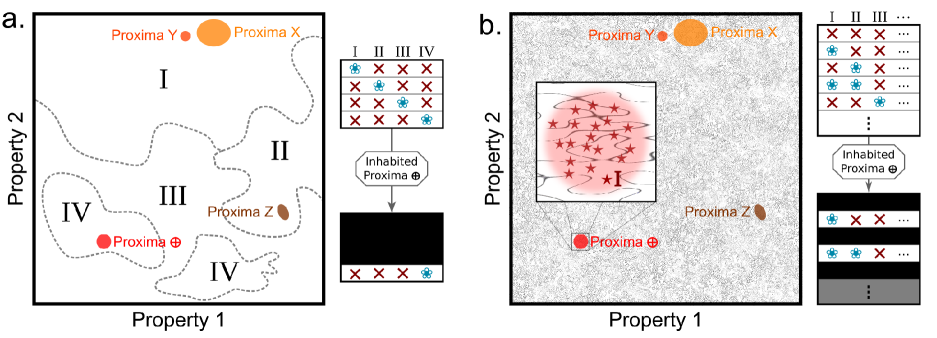
Figure 3: Extremely simplified representation of how FGAI treats theories like L-B. Probabilities of observing a particular outcome in a macrotheory may be presumed to result from some unknown fine-scale division of parameter space into regions delineating different equivalence classes. Then microhypotheses would be constructed by considering all possible outcomes for all regions. For L-B, we observe the red dwarf nearest to Earth (Proxima $\oplus$) and see whether it is inhabited (flower symbol). The observation of an inhabited Proxima $\oplus$ reduces the number of allowed microhypotheses. a.: observers on other planets distinguishable from Earth would observe red dwarfs with different properties (Proxima X, Y, and Z) and probe different classes. b.: many identical Earths observe distinct Proxima $\oplus$ (red stars). These are treated by assuming there is some indexing that allows microhypotheses to be constructed, and their likelihoods calculated by symmetry.

If we observe life on Proxima b, then the sole microhypothesis of L-A survives unscathed, but implicitly only one microhypothesis of L-B of the $10^{100}$ would survive. Thus, after the observation, L-A has a posterior credence of $100\%/(1+10^{-100})$, while L-B has a posterior credence of $10^{-100}/(1+10^{-100})$. As we would hope, FGAI predicts that we would be virtually certain that L-A is correct, which is the result we would expect if we assumed we observed a “typical” red dwarf.

What of the other inhabited G dwarf planets in an infinite Universe? The nearest red dwarfs to these will have different characteristics and most of them will belong to different equivalence classes (Figure 3). In principle, we could construct microhypotheses that specify what each type of these observers will around their nearest red dwarf, and implicitly we assume they exist. If we failed to develop the capability to determine whether Proxima b has life but aliens from 18 Scorpii broadcast to us that their nearest red dwarf has life, the result would be the same. Because we do not know what the equivalence classes are, we cannot be sure about which types of observers share equivalence classes. We might instead define equivalence class #1 to have life, and then consider each microhypothesis to be a mapping between distinct types of observer and equivalence class number.

IV.5 Fine-graining and implicit coordinate systems

The strictest interpretation of the separation of physical and indexical facts is that we cannot constrain physical models if the observed outcome happens to any observer physically indistinguishable from us. This is untenable, at least in a large enough universe – quantum mechanics predicts that all non-zero probability outcomes will happen to our “copies” in a large universe. But this would mean no measurement of a quantum mechanical parameter can be constraining. Surely if we do not observe any radiodecays in a gram of material over a century, we should be able to conclude that its half-life is more than a nanosecond, even though a falsely stable sample will be observed by some copy of us out there in the infinite universe.

Strict indeterminism is not necessary for this to be a problem, either. In the last section, we might have supposed that the existence of life on Proxima b depends on its exact physical microstate five billion years ago, and that these microstates are scattered in phase space. Yet, Proxima b is more massive than the Earth and has a vaster number of microstates – by the pigeonhole principle, in an infinite Universe, most Earths exactly identical to ours would neighbor a Proxima b that had a different microstate and could observe a different outcome about whether it has life (Figure 3).

But the separation of indexicals and physical theories need not be so strict. Indexicals are regarded in FGAI as propositions about coordinate systems. In physical theories we can and do use coordinate systems, sometimes arbitrary ones, as long as we do not ascribe undue objective significance. We can treat these situations by imposing an implicit indexing, as long as we do not ascribe undue physical significance to it. Thus, in an infinite Universe, we label “our” Earth as Earth 1. The next closest Earth is Earth 2, the third closest Earth is Earth 3, and so on. We might in fact only implicitly use a coordinate system, designating our Earth as Earth 1 without knowing details of all the rest. Our observations then are translated into third-person propositions about observations of Earth 1. The definition of the coordinate system imposes an indexical distribution where we must be on Earth 1. Of course, this particular labeling is arbitrary, but that hardly matters because we would reach the same conclusions if we permuted the labels. If we came into contact with some other Earth that told us that “our” Earth was Earth 3,296 in their coordinate system, that would not change our credence in a theory.

In a Large world, then, the microhypotheses consists of an array listing the outcome observed by each of these implicitly indexed observers. Only those microhypotheses where Earth (or observer) 1 has a matching observation survive. If the observed outcome contradicts the outcome assigned to Earth 1 by the microhypothesis, we cannot then decide we might actually be on Earth 492,155 in that microhypothesis because Earth 492,155 does observe that outcome. The coordinate system’s definition has already imposed the indexical distribution on us. Using an implicit coordinate system lets us apply a fine-graining treatment, where typicality is a consequence of combinatorics.

There are limits to the uses of implicit coordinate systems, however, if we wish to avoid the usual Doomsday argument and its descent into solipsism. In SB-B, could we not assign an implicit coordinate system with today at index 1, and the possible other day of the experiment at index 2? A simplistic interpretation would then carve the Long run theory into two microhypotheses: observer 1 is on Monday and observer 2 is on Tuesday, and observer 1 is on Tuesday and observer 2 is on Monday. Upon learning it is Monday, this fine-graining would lead us to favor the Short run theory.

There is a very important difference between SB-B and these examples. First, the number of observers is the same when deciding between L-A and L-B or in other typical experiments. Furthermore, in this section’s thought experiments, our physical theory did not in any degree predict which observers get a particular outcome. Thus the likelihood distribution over the outcomes is exactly identical for all observers. This is why we are able to assign likelihoods even though the mapping between our implicit coordinate system and some external coordinate system is unknown. In SB-B, though, our physical theory does predict which observer gets a particular outcome. The likelihood of observing “it is Monday” is not identical for each day. Instead, “it is Monday” needs to be interpreted as an indexical fact. We can indeed create an implicit coordinate system with today at index 1 and the other day at index 2. But we cannot calculate likelihoods in this coordinate system – the referents of the indices in the theory are unknown, and until we can connect the implicit coordinates with the coordinate system used by the Long theory, we cannot update credences either. All we can say is that if observer 1 is located on Monday, they observe “it is Monday” with certainty; if observer 1 is located on Tuesday, they observe “it is Tuesday” with certainty. In these kinds of situations, a more sophisticated theory is needed.

IV.6 Naive FGAI and $x$-day arguments

IV.6.1 Classes of $x$-day models in FGAI

One advantage of underpinning typicality arguments with fine-grained hypotheses is that doing so forces one to use a well-specified model that makes the assumptions explicit. In an $x$-day Argument, each microhypothesis corresponds to a possible permutation of people born as well as a complete set of possible observations by each observer (whether a human or an effectively independent external observer like an alien). This entails an observation model, a set of constraints on who can observe whom. In particular, realistic theories of observation are causal – an observer cannot “observe” people living in the future – and local – an observer cannot “observe” another person without some physical mechanism linking them.

In this section, I will discuss four general classes of fine-grained $x$-day schemas, resulting in microhypotheses with different combinatorial properties. These fine-grainings are illustrated by a simplified model where we consider only two theories [c.f., 1]: a Short/Small theory with final human population $N_{S}$ and a Long/Large theory with final human population $N_{L}$, where $N_{L}>N_{S}$. Each human at $x$-rank $r$ is drawn from a set of possible humans $H$, and measures their $x$-rank to be $r$, specifying the observation model. The possible humans in $H$ correspond to different genetic makeups, microbiomes, life histories, memories encoded in the brain, and so on. The details of how humans at rank $r$ are selected from $H$ form the basis for each of the different model classes (Figure 4).

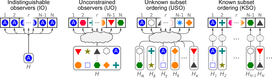
Figure 4: Different fine-grainings of the $x$-day Argument in FGAI have different assumptions about the interchangeability of humans. The four basic schema shown here correspond to IO, a Sleeping Beauty-like case where all observers are treated as indistinguishable; UO, where there are many possible humans, each of whom may be assigned to arbitrary ranks; USO, where possible humans are grouped into subsets and each rank may drawn from only one subset, although the order of the subsets is unknown; and KSO, where each rank draws from a fixed subset of possible humans, although which observer from each subset is selected is arbitrary. The clouds represent an unknown or random selection from a set. The shown configurations are chosen so that observer $A$ (blue circle) exists with rank $1$, but this is a contingent selection in the models.

The four schemas differ by their restrictions on the possible permutations:

• Indistinguishable Observers (IO) – Every possible human is treated as identical, with $H=\{A\}$. There is only one possible microhypothesis for each theory because the permutations are indistinguishable. Any information about $x$-rank is treated as purely indexical. IO is essentially the same kind of scenario as SB-B.

• Unconstrained Observers (UO) – Humans are drawn from a very large set $H$ (with $|H|={\cal N}$) of distinguishable observers, and any $h\in H$ can be born at any rank $r$. In UO, people with different names, identities, and memories could be treated as distinct members of $H$, but these details would no correlation with historical era.

• Unconstrained Subset Ordering (USO) – The set of possible humans $H$ is partitioned into ${\cal R}$ ($\geq N_{L}$) mutually disjoint subsets $H_{r}$, with one for each $r$. Humans with rank $r$ can only be drawn from $H_{r}$. This reflects the fact that individuals are the result of a vast constellation of historical circumstances that should never be repeated again. In USO, we can specify the contents of these subsets, but we do not know which subset is assigned to each $r$. In an infinite Universe, every “copy” of you will have the same $r$ as you.

• Known Subset Ordering (KSO) – As in USO, the set of possible humans is partitioned into disjoint subsets $H_{r}$, with humans at rank $r$ drawn only from $H_{r}$. Unlike USO, we already know beforehand the ordering of these subsets – which one is $H_{1}$, $H_{2}$, and so on. All that remains to be discovered is the final human population $N$ and which humans, in fact, are selected out of each $H_{r}$. KSO models emphasize how we already know, by virtue of our historical knowledge, our place in history before applying an $x$-day Argument.

None of these models exactly corresponds to how we would approach the Doomsday Argument, since we do not actually know the set $H$ or exactly how it is partitioned – these details are implicit for us. But by making explicit models, they illustrate the problems it can run into. Of these, KSO arguably is most analogous to our situation when we apply the Doomsday Argument, since humans who know they live in the year 2021 cannot be born in the Paleolithic or an interstellar future (to the extent our memories are reliable). Our Short and Long theories actually posit that everyone who has lived exist at their birthranks, and then propose an additional $N_{\rm future}$ future people after us, with the likelihood of us existing at birthrank $10^{11}$ being $1$ by assumption. This is not just a tautology because who you are is shaped by your place in history; realistic Small and Large models both predict that you, with all your personality, memories, and beliefs, could only appear this point in history [as in 26].

Although previous discussion in this paper has made it seem like there are “purely indexical” measurements, in a strict sense this cannot be true. All measurements are physical events. When someone learns their position, they are actually interacting with a physical environment that is location-dependent and changing as a result. Therefore, a truly physical theory cannot regard observers as identical if they have different indexical knowledge. Instead, such observers can only be found in specific locations. For example, hypotheses about individual $A$ of Figure 4 really should be fine-grained into hypotheses about $A_{1}$, who can only exist at rank $1$, and $A_{2}$, who can only exist at rank $2$, and so on. In this sense, USO and KSO are more physically grounded in how they interpret indexical observations than UO or IO.

IV.6.2 Self-applied $x$-day Arguments in Naive FGAI

An $x$-day Argument to constrain final population may be self-applied by a member of the population being constrained (as in the Bayesian Doomsday Argument), or applied by an external observer who happens upon the population at some time (analogous to some of Gott 11’s examples). Self-applied $x$-day Arguments are by far more problematic. Naive FGAI provides a partial – though incomplete – accounting of how self-applied $x$-day Arguments like Bayesian Doomsday fare.

I will start under a “single-world” assumption that there is only one copy of humanity in the cosmos (or that every copy of humanity yields the same exact permutations of extant humans). Then it is relatively simple to calculate the number of microhypotheses in IO, UO, USO, and KSO with combinatorial arguments, given the number of humans in $H$ (and each $H_{r}$). In Naive FGAI, the likelihoods for each macrotheory about $N$ is then given by the fraction of microhypotheses consistent with observations. Table 1 presents the results of such calculations, where the observer in question is labeled $A$ and is located at $N_{x}=1$ without loss of generality.

Table 1: Microhypotheses counts for self-applied $x$-day Arguments in single world models

	IO	UO		USO	KSO
		No replacement	With replacement	All $|H_{r}|$ equal
Total permutations	$1$	$\displaystyle\frac{{\cal N}!}{({\cal N}-N)!}$	${\cal N}^{N}$	$\displaystyle{\cal N}_{r}^{N}\frac{{\cal R}!}{({\cal R}-N)!}$	$\displaystyle{\cal N}_{r}^{N}$
Permutations where $A$ selected	$1$	$\displaystyle N\frac{({\cal N}-1)!}{({\cal N}-N)!}$	${\cal N}^{N}-({\cal N}-1)^{N}$	$\displaystyle N{\cal N}_{r}^{N-1}\frac{({\cal R}-1)!}{({\cal R}-N)!}$	$\displaystyle{\cal N}_{r}^{N-1}$
Permutations with $A$ at rank $1$	$1$	$\displaystyle\frac{({\cal N}-1)!}{({\cal N}-N)!}$	${\cal N}^{N-1}$	$\displaystyle{\cal N}_{r}^{N-1}\frac{({\cal R}-1)!}{({\cal R}-N)!}$	$\displaystyle{\cal N}_{r}^{N-1}$
Fraction where $A$ exists	$1$	$N/{\cal N}$	$1-(1-1/{\cal N})^{N}$	$\displaystyle\frac{N}{{\cal N}_{r}{\cal R}}$	$1/{\cal N}_{r}$
Fraction with $A$ at rank $1$	$1$	$1/{\cal N}$	$1/{\cal N}$	$1/({\cal R}{\cal N}_{r})$	$1/{\cal N}_{r}$

In the single world model, the four schemas all arrive at the ultimate conclusion that the surviving microhypothesis fraction if $A$ measures their rank to be $1$ is independent of $N$. In Naive FGAI, this means the $x$-day Argument is nullified in all of them. Yet they take different routes to get there. In IO, $A$ is the only possible individual, and there only ever is one microhypothesis per theory, which can never be ruled out – $A$ merely learns indexical information. In UO and USO, there is an SIA-like effect when $A$ observes themself to exist: there are more locations for $A$ to be born in the Large theory, so more microhypotheses are consistent with that observation. Unlike the SIA, this indication effect is not in the prior itself but as a result of the self-observation. Then $A$ measuring their rank of $1$ culls proportionately more microhypotheses in the Large theory, canceling this effect. Finally, in KSO, where $A\in H_{1}$ a priori, $A$’s self-observation automatically implies that $A$ is at rank $1$ no matter the theory.

We can also consider “many worlds” models in which there are many copies of humanity out the larger cosmos, each with different rank permutations of human individuals. Now there would be a distribution of lifetimes for all the humanities, but for simplicity we can consider models where historical forces (e.g., nuclear war or environmental constraints) always either end humanity in the near-future or fail to prevent its explosion into a Large interstellar future. In IO, birthrank measurement continues to be a purely indexical measurement. In the other models, the probability any given individual $A$ exists somewhere in a vast cosmos converges to $1$. In order to make any inferences in Naive FGAI, we would need to use the implicit coordinates described previously, with each $A$ labeling their world as world I and considering microhypotheses about who is at rank $1$ in world I. In KSO and USO this allows a kind of coarse-graining of the microhypotheses yielding similar results to the “single world” model.

UO yields the most ambiguous results in “many worlds”. There will exist worlds where $A$ measures themselves to have any possible rank. What $A$ infers depends on what kind of indexing scheme they use. If they index only over worlds, then $A$ is more likely to exist in world I’s history in a Large $N$ model, balanced by being less likely to exist at rank $1$. But previous discussion of these implicit coordinate systems suggest $A$ should index over their copies: not worlds in general, but only worlds containing observers identical to themself. Then, because $A$ is guaranteed to exist in a vast enough cosmos, there is a Doomsday Argument. Any given $A$ is more likely to observe themself at rank $1$ if there are fewer possible ranks they could be born at, as in the Short histories. Note, however, in practice this requires anachronistic birth orders with any individual being born with equal frequency in every epoch in history. There would have to actually be as many worlds where you specifically, with all your memories, would be the first human as ones where you live in 2021 – a physically improbable outcome and thus incompatible with the spirit of FGAI. This anachronism is prevented in USO and KSO, which have no Doomsday effect even in a vast cosmos.

IV.6.3 Externally-applied $x$-day arguments in Naive FGAI

Externally-applied $x$-day Arguments are structurally similar to “urn” thought experiments, while seeming to also justify the self-applied Doomsday Argument by analogy. Under some circumstances, one can infer something about the lifespan distribution of an external phenomenon by drawing a sample of it at random (as in the most popularized examples of Gott 11). But the key difference with self-applied Doomsday arguments is the existence of an additional “observer” that is the one carrying out the experiment, who is completely outside the population being constrained. This adds another physical degree of freedom, which changes the microhypothesis counts in Naive FGAI to allow for a Doomsday Argument.

Suppose an observer $X$ happens upon humanity, with individuals drawn from $H$ according to IO, UO, USO, or KSO. All of the possible sequences of human individuals listed by the microhypotheses still are valid, and would have the same relative prior probabilities. Yet there is a final observable quantity, which is actually what $X$ measures: the relative time $t$ between humanity’s start and $X$ happening upon us. Even if the evolution of $X$ is deterministic enough to demand they arrive at a specific time, $X$ does not have enough information beforehand to select a particular $t$; presumably such factors are microscopic and chaotic. Therefore, every single one of the microhypotheses of the previous section must now be divided into $T$ even finer microhypotheses, one for each possible $t$ interval $X$ can arrive in.

Whether a Doomsday Argument applies depends on the selection process, in particular how $X$ found humanity. If $X$ could plausibly have arrived before or after humanity’s existence, then $T$ is both much larger than humanity’s lifespan ${\cal T}_{H}$ (or its equivalent) and also independent of ${\cal T}_{H}$. This selection method is quite common: if one looks for examples of a rare phenomenon at a particular location, then most likely one will be searching in the vast epochs before or after it passes. It is in fact less of a coincidence for $X$ to arrive at the right time to observe humanity if $N$ is large, favoring a Large history – the fraction of surviving microhypotheses scales as $\sim{\cal T}_{H}/T$. Now suppose $X$ measures the age of humanity. The fraction of microhypotheses consistent with $X$ arriving at this particular epoch of human history ($\sim 1/T$) is the same in Small and Large models. Thus there is no Doomsday Argument as such; $X$ cannot constrain humanity’s lifespan.

But what if there is no possibility of $X$ failing to make an observation of humanity? One could suppose that rather than searching a particular location, $X$ seeks out the nearest technological society, scouring the infinite cosmos if they have to until they find one. (We will also assume all such societies have exactly the same lifespan for the sake of argument.) This would be more like picking someone on the street to ask them their age. The only possible values of $t$ are values within humanity’s lifespan – each Large history theory has a larger number of possible outcomes. The microhypothesis counts in Table 1 are multiplied by $N$ to account for the extra degree of freedom in $t$. Only $\sim 1/{\cal T}_{H}$ of them are consistent with any particular measurement of humanity’s current age. In FGAI, $X$ now favors Small histories, and the externally-applied Bayesian Doomsday argument is in effect.

These are not the only possible models for the time of $X$’s arrival. Actual observations may deliberately be carried out at a specific time during its history, limiting the microhypotheses about $t$ to a narrow range independent of ${\cal T}_{H}$ [as in the wedding example of 49]. Furthermore, the age of the Universe sets an upper limit on the relative $|t|$. We cannot rule out astrophysical objects having lifespans of trillions of years – as we suspect most do [50]. Finally, the observational outcomes will be biased if the population varies with time. If we survey an exponentially growing population of human artifacts, for example, Gott [11]’s Doomsday Argument necessarily underpredicts the lifespan.

V Reconstructing typicality

V.1 The indication paradox in Naive FGAI

Naive FGAI, supplemented by the use of implicit microhypotheses and implicit coordinate systems, is sufficient to handle many practical cases where typicality is invoked. It also suggests at least one route for addressing the Doomsday Argument, KSO. As noted, though, it sometimes favors Large theories where a specific individual is more likely to exist. Now, sometimes this can be a reasonable assumption. Suppose SB-B was being carried out not with one participant, but two already extant observers, Alice and Bob, who remember their pre-experiment lives. Further suppose one was chosen at random to be wakened on each day, and both wake up at the end. If Alice wakes in the experiment, she plausibly can conclude the Long version of the experiment is more likely because she then would be more likely to be awakened. But would it really make sense if a new participant is instead created each day with no memories and never waking up again?

Allowing for this SIA-like effect can lead to bizarre consequences. Consider this compounded version of SB-B:

• (SB-B^′) You wake up in the room. The experimenters tell you they are running SB-B, but each day they will also flip a fair coin each day the experiment is run and tell you the result. But a team member gains your trust and tells you they are lying! The other experimenters have either adopted Strategy A or Strategy B. In Strategy A, they tell you the coin lands Heads on Monday, and if you awaken on Tuesday, they will tell you it landed Tails. In Strategy B, the supposed outcomes are opposite Strategy A’s. Suspecting your new friend’s duplicity, the other experiments exclude them from the decision of which Strategy to go with. Now the experimenters inform you the coin landed Heads. How does that affect your credence in a Short or Long run?

It is obvious the coin flip “result” should not affect our beliefs in a Short or Long experiment, because of the symmetry between the coin flip outcomes. Yet in Naive FGAI, either coin flip “result” leads us to favoring a Long experiment (Figure 5)! The reason is that in the Long experiment, you will experience each outcome at least once in either Strategy’s microhypothesis, but only one of the two Strategies in the Short theory results in a Heads “observation”. Thus only one Short microhypothesis survives compared to both of Long’s.

The indication paradox is that any datum about the false coin flip favors the Long run. It is analogous to asserting that since your existence is the result of innumerable unlikely factors, the Universe is surely very large given that you as a specific individual do in fact exist.

V.2 Revising FGAI to confront the paradox

This is the fundamental issue: how should we calculate likelihoods when we don’t even know who or where we are? When discussing Naive FGAI, there was a symmetry between the observers being considered in that all of them genuinely had equal probabilities distributions for observed outcomes. But in cases like SB-B and SB-B^′, otherwise identical observers at different locations necessarily observe different outcomes. There is no symmetry to exploit. Naive FGAI simply used the maximum likelihood among all possible observers, but this is not the only possible solution. The results of applying other formulations of FGAI to SB-B^′ are illustrated in Figure 5.

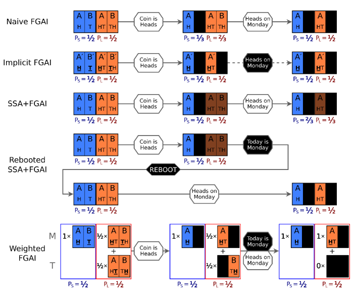
Figure 5: The indication paradox of SB-B^′, and how it is treated with different modifications of FGAI. Each box, representing the credence in a microhypothesis, lists the observed outcomes, ordered by index in the used coordinate system. An underlined, bold outcome is treated as the one the observer measures for the purposes of calculating likelihoods. In the Weighted FGAI treatment, the normalized weights applied to each microhypotheses are given to the left of each provisional physical credence.

Implicit FGAI – The solution closest to Naive FGAI is labeled Implicit FGAI, because we reject the formulation of SB-B^′ and adopt an implicit coordinate system referring to “today” and “the other day”. We then fine-grain according to mixings of the pure Strategies A and B: we instead consider Strategies A^′ and B^′. In Strategy A^′, the experimenters tell us the coin lands Heads today and Tails on the “other day” if we awaken on “the other day”; in Strategy B^′, the outcomes of A^′ are flipped. In this situation, a Heads “observation” today rules out both B^′ microhypotheses, preventing an indication effect. A further observation that “today is Monday” is treated as purely indexical, with no relevance for our physical credences.

We can use the symmetry to perform a “coordinate transformation” between strategies referring to external labels and strategies referring to our labels. In this case, the symmetry is restored in the participant-centric coordinates, but this is not generally possible – if our friend told us at the start the experimenters had decided on Strategy A, there would be only one allowed microhypothesis in Short, but two in Long, leading to a Doomsday-like effect. Without this symmetry, implicit FGAI does not let us translate predictions from one indexical system to another, severely limiting its use. Labels like “Monday” or “Tuesday” are meaningless until one can connect them to the implicit coordinate system, propositions like “Strategy A is adopted” or “Strategy B is adopted” lack the referents to connect them to observations. Because of this inability, Implicit FGAI is inadequate.

SSA+FGAI: Doomsday without solipsism? – A more radical solution is to reintroduce the SSA: instead of applying the maximum possible likelihood for an outcome among all observers we might be, we applying the mean likelihood among these possible observers. Equation 6 is modified to:

$$P^{\rm pos}_{k,j}=\frac{\displaystyle P^{\rm prior}_{k,j}\times\sum_{i\in O_{k,j}(D)}\frac{{\cal L}(\mu_{k,j}|o@i\to D)}{|O_{j,m}(D)|}}{\displaystyle\sum_{x=1}^{M}\sum_{y=1}^{m_{k}}P^{\rm prior}_{x,y}\times\sum_{z\in O_{x,y}(D)}\frac{{\cal L}(\mu_{x,y}|o@z\to D)}{|O_{x,y}(D)|}}.$$ (8)

Then, in SB-B^′, the result of the “coin flip” does not affect our credences in Short and Long. Both microhypotheses of Long would survive the observation, but they would be penalized by a $1/2$ factor because only one in two participants is given a Heads outcome. But this penalty continues to apply even when it is no longer needed: when we now apply the observation that “today is Monday” (and thus Strategy A was adopted) to the resulting distribution, Short is now favored two to one.

Although the SSA+FGAI provides a route for the Doomsday Argument in FGAI, this may not be as bad as it seems. The fine-graining “tames” the unrestricted SSA’s solipsistic tendencies in many cases, when there is no “ranking”: note that in SB-B^′, we disfavor the Long hypothesis only after we learn it is the first day of the experiment. The frustration of solipsism is illustrated by a minimal model in which we consider possible extant observers $A$ and $B$, with a Small world theory that only one of them exists and a Large world theory where both exist. In the Small world model, the two microhypotheses are only $A$ existing and only $B$ existing. But in the Large world model, because there is no ordering, there is only one microhypothesis: both $A$ and $B$ exist. Thus, $A$’s self-observation allows one of two Small microhypothesis with its full weight and the sole Large microhypothesis with just half weight to survive, leaving Small and Large with equal credence. No further data is possible, and thus Small and Large remain in equal standing.

This is the crucial difference between the Doomsday Argument and the other solipsistic arguments that SSA+FGAI exploits. When considering $x$-day Arguments, it is impossible for observers with high $N_{x}$ to exist without observers with low $N_{x}$ also existing. It would be like if the Small world model only had the microhypothesis that $A$ exists. When considering other solipsistic thought experiments, we can include hypotheses that only observers unlike us exist in our Small theory prior – microhypotheses where only fish are conscious instead of humans, or only Jupiter is inhabited instead of Earth. Indeed, we must include them to avoid solipsism, although these possibilities usually are not included when “Copernican” arguments are made. Even Doomsday itself may be neutralized in the KSO model if we apply the SSA to the narrow reference class of observers identical to ourselves: every microhypothesis where we exist has us living in 2021.

Despite being “tamer” than unrestricted SSA, SSA+FGAI is unsatisfactory both in that it allows (potentially unrealistically powerful) Doomsday Arguments at all and because it never “forgives” the penalties it imposes. Recall, the $1/2$ factor applied to Long’s likelihood in SB-B^′ arose from the fact that you could plausibly either be awake then on Monday or Tuesday. Because of your indexical uncertainty, you had no way to assign one value to the likelihood, and the SSA’s purpose was to provide it in the face of this ambiguity. That circumstance no longer applies if you then learn “today is Monday” and the indexical uncertainty is eliminated, but there is no way to undo the SSA. Essentially, this results in SSA+FGAI double-counting the evidence against Large theories: penalizing all the microhypotheses because we do not know who we are, and then penalizing some of the microhypotheses because we do know who we are. In contrast, if you had learned “today is Monday” first, then you would have had enough indexical information to calculate a single likelihood for each microhypothesis. SSA+FGAI is unsatisfactory because it either reaches different conclusions based on which order data is learned, or it demands the widest possible reference class always be used no matter what we learn.

Rebooted SSA+FGAI – “Rebooted SSA+FGAI” is a modification of SSA+FGAI to eliminate the order-dependence of learning data. It is like SSA+FGAI, except that the credence distribution is reset to the original prior whenever new indexical information is learned. Then, all physical and indexical data is re-applied simultaneously. The likelihood of microhypotheses are evaluated according to the SSA applied only among observers with all your current indexical data. Essentially, with each reboot, the reference class shrinks. The rebooting undoes the penalty applied by the SSA.

V.3 Weighted FGAI

The most advanced of the FGAI frameworks is Weighted FGAI. Like Rebooted SSA+FGAI, Weighted FGAI effectively allows re-evaluation of likelihoods as new indexical information is learned. It also provides a more formal framework for keeping track of indexical information.

Weighted FGAI’s premise is that there is no single physical distribution for the microhypotheses. Instead, every microhypothesis has many physical credences, one for each possible observer location. These are the provisional physical credences, each evaluated as if we were certain that we were at its associated location. The set of provisional physical credences is then bound by a set of indexical weights, which is an indexical distribution evaluated according to the indexical knowledge we have. At any given time, we evaluate our credences in the various microhypotheses by averaging over the provisional physical distributions using the indexical weights.

In Weighted FGAI, we consider the set $O$, collecting every possible observer-trajectory among all the microhypotheses in each macrotheory. Within each macrotheory $\tau_{k}$, each possible observer-trajectory $i$ we might be located on has an indexical weight $w_{k,i}$. In real experiments, we may know enough to eliminate some possible observer-trajectories, so these are excluded from $O$ (e.g., we restrict $O$ to humans). Note that all microhypotheses in each macrotheory share these weights, but they are not shared between macrotheories (see Section V.5). Only some subset $O_{k,j}$ of $O$ are possible observer-trajectories in a given microhypothesis $\mu_{k,j}$, and each $\mu_{k,j}$ has its own normalization for the weights: ${\cal W}^{\rm pos}_{k,j}\equiv\sum_{i\in O_{k,j}}w^{\rm pos}_{k,i}$. In the absence of any prior data or other constraints on uninformative priors, the weights are initialized with an uninformative distribution $w^{\rm prior}_{k,i}=1$. This is the effective role of the SSA in Weighted FGAI – it is the principle for choosing initial indexical weights.

The provisional physical credence $p_{k,j,i}$ is the credence in $\mu_{k,j}$ calculated by an observer along observer-trajectory $i\in O_{k}(D)$. They are not normalized, since that would require the indexical weights that are calculated for other microhypotheses, and are not true probability distributions, although they are closely related to actual physical credence distributions. Unless otherwise required based on prior knowledge or to ensure an uninformative credence distributions (Section V.7), initial prior credences at all observer-locations are assigned as in Naive FGAI: $p^{\rm prior}_{k,j,i}=P^{\rm prior}_{k,j}$.

We update the provisional physical distributions when observations when an observation give us data $D$. For each microhypothesis, the observation model combined with the assumption that we are the observer along trajectory $i$ yields a single likelihood for that data. The provisional physical distributions are thus “updated” using these likelihoods, neglecting normalization: $p^{\rm pos}_{k,j,i}=p^{\rm prior}_{k,j,i}\times{\cal L}(\mu_{k,j}|o@i\to D)$. As in Naive FGAI, the provisional physical distributions are insulated from indexical information.

The data may also yield indexical information – if we learn “today is Monday”, “I am a human on Earth”, or “my birthrank is 108 billion”, for example. The indexical weightings is updated independently according to the probability we have data $D$ if we are the observer along trajectory $i$, averaged over the macrotheory’s microhypotheses:

$$w^{\rm pos}_{k,i}=w^{\rm prior}_{k,i}\frac{\sum_{j:i\in O_{k,j}}p^{\rm prior}_{k,j,i}P(o@i\to D|\mu_{k,j})}{\sum_{j:i\in O_{k,j}}p^{\rm prior}_{k,j,i}}$$ (9)

In situations like SB-A when we already are certain of the physical nature of the world, $p^{\rm prior}_{k,j,i}$ is nonzero only for the known world model $\mu_{k,j}$. In that case, $w^{\rm pos}_{k,i}$ is an unnormalized indexical credence and equation 9 reduces to normal Bayesian updating. The Bayesian limit more generally occurs if $P(o@i\to D|\mu_{k,j})$ is the same for all remaining microhypotheses. Indexical data can be neutral with respect to the different locations. In other cases, we may learn exactly which observer we are (such as “My birthrank is exactly 108 billion” in a Doomsday Argument), resulting in a nonzero weight for a single observer-trajectory because the likelihoods for all others are zero.

Our posterior credence in microhypothesis $\mu_{k,j}$ is then generated from the provisional physical distributions by applying the indexical weights:

$$P^{\rm pos}_{k,j} =\frac{\displaystyle\frac{1}{{\cal W}^{\rm pos}_{k,j}}\sum_{i\in O_{k,j}}w^{\rm pos}_{k,i}p^{\rm prior}_{k,j,i}{\cal L}(\mu_{k,j}|o@i\to D)}{\displaystyle\sum_{x=1}^{M}\sum_{y=1}^{m_{x}}\frac{1}{{\cal W}^{\rm pos}_{x,y}}\sum_{z\in O_{x,y}}w^{\rm pos}_{x,z}p^{\rm prior}_{x,y,z}{\cal L}(\mu_{k,j}|o@i\to D)}$$ (10)

$$=\frac{\displaystyle\frac{1}{{\cal W}^{\rm pos}_{k,j}}\sum_{i\in O_{k,j}}w^{\rm pos}_{k,i}p^{\rm pos}_{k,j,i}}{\displaystyle\sum_{x=1}^{M}\sum_{y=1}^{m_{x}}\frac{1}{{\cal W}^{\rm pos}_{x,y}}\sum_{z\in O_{x,y}}w^{\rm pos}_{x,z}p^{\rm pos}_{x,y,z}}.$$

The posterior credence $P^{\rm pos}_{k}$ of a macrotheory is once again found by summing the credences of its microhypotheses. The use of the weights means that Weighted FGAI is not a strictly Bayesian theory. We cannot calculate the “actual” physical credence until we can assign a single, unambiguous likelihood, and we cannot do this in FGAI. Instead the posterior credence is a construction built from possible physical credences using the indexical weights.

Equation 10 can be viewed as Weighted FGAI’s rendition of the Observer Equation proposed by Bostrom [2]. It has several useful limits. First, if the likelihood ${\cal L}(\mu_{k,j}|o@i\to D)$ is the same for all remaining possible observer trajectories $i$ ($W^{\rm pos}_{k,i}>0$) in each microhypothesis, then this application reduces to Bayes’ formula applied on the indexical weight-averaged prior probabilities. In particular, in situations where indexical information is entirely irrelevant, $p^{\rm prior}_{k,j,i}=P^{\rm prior}_{k,j}$ and all indexical dependence vanishes from equation 10. Second, suppose the data $D$ picks out a subset $O^{\prime}\subset O$ possible observer-trajectories, but is equally consistent with all of them. Then, $O^{\prime}$ is our location reference class, and equation 9 applied to equal prior weights yields an equal prior weight for each element in $O^{\prime}$. This amounts to an assertion of the SSA applied to the narrowed reference class $O^{\prime}$. Equation 10 then implements SSA+FGAI (equation 8). Of course, if we know our exact observer-trajectory, then that trajectory’s indexical weight is $1$, and we are left with Bayes’ formula with likelihoods calculated using our known location. Finally, if we are already certain that $\mu_{k,j}$ is correct, then the prior provisional credences are nonzero only for this microhypothesis, and equation 10 gives $P^{\rm pos}_{k,j}=1$.

As required in FGAI, the indexical weights are entirely separated from the (provisional) physical distributions, albeit with a more active role than in Naive FGAI. The weights shift adaptively in response to indexical data, as we can more accurately assess likelihoods over microhypotheses. The novel feature of Weighted FGAI is the shifting indexical weights’ ability to “revive” theories that were provisionally disfavored by the SSA. This lets us implement the “rebooting”, where we evaluate all the likelihoods again with fresh indexical knowledge. If we had only a single joint probability distribution, evidence can only eat away the prior probability in a theory because likelihoods are always $\leq 1$. The only way a theory survives with a single credence distribution is if the other theories’ prior credence is also consumed at a comparable rate. In Weighted FGAI, the provisional probability invested in disfavored observer trajectories is not lost but re-assigned to the microhypotheses consistent with likely observer trajectories.

This formulation of Weighted FGAI is based on the assumption that there are only a finite number of locations or trajectories, parameterized by a finite set of indexical weights. Infinite volumes are a common feature of modern cosmologies, however. One way to address this problem would be to replace the discrete distributions with densities in a way that recovers conclusions found for an arbitrarily large finite number of locations. Another is to note that the number of expected configurations of a Hubble volume is expected to be finite [e.g., 51]. The ultimate motivation for including the weights is that likelihood calculations depend on observer-trajectory and evolution. If two locations are located in two indistinguishable Hubble volumes, their likelihood calculations should also be indistinguishable. Because the weights would no longer refer to a single location with a unique evolution, trouble could arise if all observations are be explained away by “updating” to whichever unlikely sequence of Hubble volume configurations just happens to fit the data. We might prevent this by allowing indexical updates solely on information available in the past light cone when observations begin. This would let us update indexical information to account for our birthrank or our location in a spiral galaxy, for example, without letting us pretend that we just happen to be in the Hubble volume where all observed positrons have remained stable despite having a half-life of a femtosecond.

V.4 What are the indexical weights?

The indexical weights probabilistically define our current reference class, which evolves as we learn new information. These weights are calculated using likelihoods averaged over all microhypotheses. But who is doing the observation along that trajectory depends on the microhypothesis, just as who is born at birthrank $1$ in the Doomsday Argument varies. Thus the indexical weights describe a reference class of locations or contexts (or more properly, trajectories), not observers. The indexical weights tell us where we are, not who we are.

Equation 9 includes a dependence on the prior physical credence $p^{\rm prior}$. When normalized, the indexical weights themselves form a joint physical-indexical probability distribution, even though weighted FGAI rejects such distributions for the physical credence. Unlike previous joint distributions, the indexical weights implement an inverse SSA. Instead of evaluating physical hypotheses under the assumption we are a typical observer, it evaluates indexical hypotheses under the assumption that a typical physical hypothesis within a macrotheory is true.

Indexical weights can also be viewed as a second-order probability distribution over a series of trivial indexical distributions. Srednicki and Hartle [32] first proposed that we could test the correctness of various indexical distributions called xerographical distributions by comparing their predictions in physical theories with our evidence. A key difference with Srednicki and Hartle [32], though, is that only an orthonormal set of xerographic distributions, each implying absolute certainty in one’s trajectory, is used in Weighted FGAI.

Unlike the attached indexical distributions of Section III, the indexical weights are averaged over all possible microhypotheses. The indexical weights can be non-zero for locations completely inconsistent with the data – indeed, this is how Weighted FGAI is able to constrain these microhypotheses at all. If we are just interested in the indexical distribution for a single microhypothesis, it can be calculated as:

$$\xi_{k,j,i}=\frac{w^{\rm prior}_{k,i}p^{\rm prior}_{k,j,i}P(o@i\to D|\mu_{k,j})}{\sum_{z\in O_{k,j}}w^{\rm prior}_{k,z}p^{\rm prior}_{k,j,z}P(o@z\to D|\mu_{k,j})}.$$ (11)

One unresolved issue is what counts as a separate trajectory. If the experimenters in SB-B^′ assigned you to room I if they chose Strategy A but room II if they chose Strategy B, or if they put you in room I on the Heads day and room II in the Tails day, different hypotheses about strategies naively have their own indexical weights. This leads to an SIA-like effect, even if the rooms are completely indistinguishable from your perspective (see also Section V.7). A deeper understanding of locations and trajectories in Weighted FGAI is needed to resolve the issue, however.

V.5 How should the indexical weights be linked?

According to equation 10, the weights are shared among all microhypotheses and all macrotheories, but is this necessary?

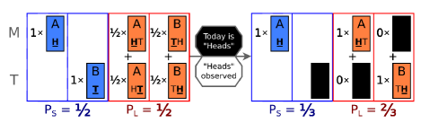
Figure 6: Illustration of how using microhypothesis-level weighting in SB-B^′ results in the indication paradox where any data about the “coin flip” automatically favors the Long theory.

Perhaps the most natural solution would be to give each microhypothesis its own set of weights, updated according to equation 11. This scheme is invalid: the averaging of the weights regulates how much each weight can “adapt” to new data. Microhypothesis-level weights are too sensitive – they find whichever observer happens to have your data $D$ and declare that you are that observer. In a large enough universe, there is likely to be some observer at some location with your data $D$, and the result is credence evaluation according to this optimal location, resulting in a likelihood of $1$. It would be like flipping a coin a thousand times, always getting heads, and then concluding that the coin is fair but you just happen to be the fluke observer who will happen to observe a thousand heads in a vast cosmos (c.f. Section IV.5). Figure 6 illustrates what happens when microhypothesis-level weights are used to resolve SB-B^′: the observer automatically favors the Long theory upon learning the “result” is Heads because a Heads observation is more likely to exist somewhere within the Long theory.

Another natural solution would be to share indexical weights between macrotheories. Indexical weights would be updated as in equation 9 by averaging over all possible microhypotheses in every macrotheory where the observer-trajectory exists. When the probability of an observer along trajectory $i$ observing data $D$ is independent of macrotheory, macrotheory-level weighting gives the same results as universal weights. Universal weights are problematic because the averaging depends on macrotheory credences themselves. Suppose in SB-B, we woke up and then learned the experimenters had chosen to run the Long variant without learning what day it was. With universal weights, we would update the Monday weight to $w_{M}=1/2$, resulting in us favoring it being Tuesday.

How weights are shared determines how “aggressive” Weighted FGAI is in making conclusions. Imagine there is an experiment with two indistinguishable participants in two rooms, both of which contain a coin. The participants watch a coin flip and observe its results but are not allowed to inspect the coins. In variant A of the experiment, both coins are fair, but in version B, room I’s coin always lands on Heads. Both variants are given equal prior credence. The microhypotheses list the possible outcomes of each coin flip in each variant. Not knowing which room they are in ($W^{\rm prior}_{\textrm{I}}=W^{\rm prior}_{\textrm{II}}=1/2$), one participant observes their coin lands Heads. How should the participant update the indexical weights?

If both variants A and B have their own weights, then the participant may update their variant B weights to $W_{B,\textrm{I}}=2/3$ and $W_{B,\textrm{II}}=1/3$, while the variant A weights are unaffected. Then the participant evaluates $P^{\rm pos}(B)=5/8$. But if there is just one set of weights for both A and B, they are instead updated them to $w_{\textrm{I}}=1/2\times(2/8+2/4)=3/8$ and $w_{\textrm{II}}=1/2\times(2/8+1/4)=2/8$. The resulting evaluated credence in variant B is $P^{\rm pos}(B)=(3/5\times 2/4+2/5\times 1/4)/[(3/5\times 2/8+2/5\times 2/8)+(3/5\times 2/4+2/5\times 1/4)]=8/13$. Linking the weights on the macrotheory-scale results in a faster convergence to the belief that one is in room I and variant B is being run.

This remains another open issue in Weighted FGAI, without an entirely clear justification for sharing weights on the macrotheory-level aside from the fact that it gives us the “right” answers.

V.6 Weighted FGAI and Sleeping Beauty

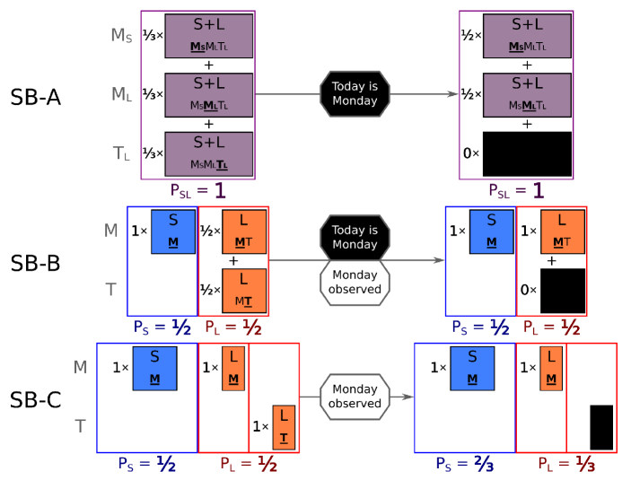
Figure 7: Treatment of the fundamental variations of the Sleeping Beauty problem in Weighted FGAI. In SB-A, only the indexical weights shift, while in SB-C, the physical credence distributions entirely drive the conclusion. In SB-B, the indexical information shifts the indexical weights assigned to each provisional distribution, ensuring that neither the Short nor Long distributions are favored.

Weighted FGAI’s treatment of the Sleeping Beauty examples is illustrated in Figure 7. Because both the physical provisional distributions and indexical weights are updated according to Bayes’ equation (as required by Section III.3), we can recover the naive Bayesian predictions of SB-A and SB-C.

In the SB-B variant, there are only the Short and the Long theories, with one trivial microhypothesis each, and each having $1/2$ prior credence. The Short theory has a normalized indexical weighting of $1$ for Monday. The Long theory has a Monday provisional probability and a Tuesday provisional probability, both still equal to $1/2$. The Long theory also has an indexical weighting of $1/2$ for Monday and $1/2$ for Tuesday. Now we learn “today is Monday”. The likelihood that this observation is made is $1$ if we are the Monday observer so the Monday provisional probabilities have a likelihood of $1$. The likelihood this observation is made is $0$ if we are the Tuesday observer, so the Tuesday provisional probability in the Long theory is eliminated. However, the Long theory gives us 100% confidence in our being the Monday observer if today is Monday, and its indexical weights shift to $1$ for Monday and $0$ for Tuesday. As a result, the probability lost in the Tuesday provisional distribution is irrelevant. Our credence in the Long theory is $(1\times 1/2+0\times 0)/[(1\times 1/2)+(1\times 1/2+0\times 0)]=1/2$, just as before.

The fine-grained perspective of FGAI and the use of observer-trajectories actually lets us differentiate between Alice and Bob being created each day and Alice and Bob being pre-existing observers. In the former, the trajectories begin and end on the same day no matter who awoke on Monday and who might be awake on Tuesday. There are thus just two indexical weights, and both describe valid locations in both Long microhypotheses. Hence, Alice’s credence in Long upon awakening is $1/2$ as in SB-B. But if Alice and Bob are pre-existing observers who remember their pre-experiment life, then the trajectories are not the same. In the Alice-first Long microhypothesis, the Monday trajectory connects with Alice’s Sunday location instead of Bob’s Sunday location. There are thus four possible indexical weights, and each microhypothesis is compatible with only some of them. It can then be shown that Alice evaluates her credence in Long as $2/3$ upon awakening. This distinction is in line with the intuition provided in the beginning of the section.

V.7 Paradoxical SIA-like effects in Weighted FGAI?

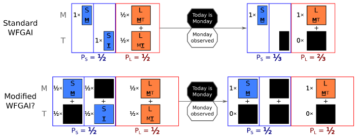
Figure 8: Illustration of a second indication paradox resulting from SB-B^′′, where the day we wake up in the Short variant is unknown. Whether we are told it is Monday or Tuesday, we favor the conclusion we are in the Long experiment (top). A modification of Weighted FGAI where both Short microhypotheses inherit the full prior credence but are weighted would evade the paradox (bottom).

Unfortunately, while Weighted FGAI evades some paradoxical indication effects, like those arising in SB-B^′, it still results in favoring Large hypotheses under other circumstances. Suppose we were participating in this modification of SB-B:

• (SB-B^′′) You wake up in the room. The experimenters tell you they are running SB-B, but if the run is Short, they then decide whether to wake you on Monday or Tuesday. Either possibility is equally likely from your perspective. The experimenters then truthfully inform you it is Monday. How does that affect your credence in a Short or Long run?

As illustrated in Figure 8, learning that it is Monday results in you favoring the Long variant because it is then more likely that an observation will be made on Monday. Just like SB-B^′, the paradox arises because any data results in you favoring the Long variant; you would reach the same conclusion if you were instead told it was Tuesday.

SB-B^′′ is not simply an isolated thought experiment with no connection to the real world. It models cases where we want to constrain non-humanlike intelligences like those living around red dwarfs or elsewhere in a landscape, starting from a state of no knowledge. It is unclear how Weighted FGAI should be modified to prevent this conclusion without opening it back up to Doomsday-like effects. SSA+FGAI avoids the problem at the cost of favoring Small models under other circumstances. A modification to the priors that lets each Small microhypothesis inherit the full macrotheory credence in different provisional distributions, trading $p^{\rm prior}$ and $w$, does not have this problem (Figure 8, bottom). This would let us construct the provisional prior credences from the uninformative distribution we would adopt if we knew our indexical location. Defining the rules for which provisional priors and weights should be used, and their motivations, remain an issue for Weighted FGAI.

V.8 Counterintuitive results with unreliable measurements?

In the examples I’ve considered, the indexical measurements have been assumed to be perfectly reliable, giving likelihoods of either $0$ or $1$ for allowed sets of locations. This has led to the conclusion that credence in a theory does not depend on how big it is. Actually, if the indexical measurements are unreliable, we do find Doomsday-like effects in Weighted FGAI for certain scenarios.

Suppose in SB-B, we know the experimenters are devious when they announce what day it is. If it is a Short experiment, then they will (correctly) tell us it is Monday. In a Long experiment, however, they will tell us the correct day only $p$ of the time and give us a wrong day with probability $1-p$. The Long theory thus has four microhypotheses about what days they will announce. When we hear the experimenters announce that today is Monday, our Long indexical weights update to $p$ for Monday and $1-p$ for Tuesday, but the provisional distributions also update. Then Weighted FGAI implies our credence in the Long theory is $1-[2(p^{2}-p+1)]^{-1}$, reaching a minimum of $1/3$ for $p=1/2$.

The decreased credence in Long is not necessarily a flaw. Arguably, if $p=1/2$, the announcement effectively acts like a randomized measurement in the Long theory but deterministic in a Short theory, so maybe we should accept the lower odds. At the same time, we may worry that we are “double-dipping” by updating both the indexical distribution and the provisional distributions. This has not been a problem before since in previous scenarios the likelihoods have been either $0$ or $1$, so squaring the likelihoods does not matter. Not updating the indexical weights always leads to $P^{\rm pos}_{L}=1/3$ upon being told it is Monday, however, even if $p$ is $0$ or $1$.

V.9 Self-applied $x$-day Arguments in Weighted FGAI

If we accept Weighted FGAI as a theory of typicality, we can easily treat self-applied $x$-day Arguments using the fine-grainings of Section IV.6.1. Each $N_{\rm total}$ macrotheory has its own set of indexical weights. In the single world versions, the observer-trajectories for these indexical weights are simply each possible $x$-rank $0$ to $N_{\rm total}-1$. In multiple world versions, there is an observer-trajectory for each $x$-rank and each world. These weights are initialized to be equal for each possible observer-trajectory. Every human can learn their $x$-rank but not which of the worlds they live in.

The single-world IO case is equivalent to SB-B: learning one has an $x$-rank of 1 shifts the indexical weights in the Long theory and the credences do not change. In a many world case where all worlds have the same $N_{\rm total}$, there is uncertainty about which world one is in, but the symmetry results in the same conclusion. If there are many worlds and we consider theories where $N_{\rm total}$ is assigned randomly, we get a series of microhypotheses about which worlds are Small and which Large. A self-observed $x$-rank of 1 zeroes out the indexical weights for all positions with $N_{x}>1$ in every world, inhibiting the Doomsday Argument just as for the single-world case.

For UO and USO, Weighted FGAI prevents the conclusion that we live in a long history simply because any specific individual is more likely to be born. The indexical weights are initialized evenly for all observers, and the observation of one’s existence provides no indexical information to change that. Thus, although the amount of prior credence that survives the self-observation is greater by $N_{\rm total}$ in a single world, it is weighted by a factor of $1/N_{\rm total}$, as only that fraction of individuals has that specific self-data. Upon learning your $x$-rank, large $N_{\rm total}$ theories are penalized by having fewer microhypotheses survive, but this is compensated by the indexical weights shifting to locate you at your actual $x$-rank. Thus you can conclude nothing from the self-applied $x$-day Argument. A worked example is given in Appendix B.

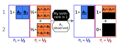
Figure 9: Illustration of how a self-applied Doomsday Argument fails in the KSO schema according to Weighted FGAI. Two models are compared, with $N_{S}=1$, $N_{L}=2$, $H_{1}=\{A_{1},B_{1}\}$, and $H_{2}=\{A_{2},B_{2}\}$. The combinatorial properties of the microhypotheses, aided by the shifting indexical weights, ensure the prior is unaffected by an observer learning they are $A_{1}$ at rank $1$.

KSO proceeds more simply because learning your individual identity also allows one to assign your $x$-rank with certainty in all microhypotheses. The self-observation eliminates the same fraction of prior weight in all theories for observers with your $x$-rank (Figure 9). The self-applied $x$-day Argument is again rendered powerless.

Weighted FGAI, with its emphasis on observations as physical events, requires exactly specified (if simplified) models instead of simply relying on analogies. Purely indexical problems, like SB-A or Leslie’s “emerald” thought experiment, do not accurately model the Doomsday Argument. Nor do purely physical problems like SB-C, urn problems, or the external Doomsday Argument (Figure 7). It is now clear why the self-applied Doomsday Argument never yields new information within Weighted FGAI:

• Indexical facts do not directly constrain physical distributions – The separation between indexical and physical distributions in Weighted FGAI shrinks reference class, retroactively shrinking the power of the $1/N_{\rm total}$ likelihoods, averting solipsism.penalizing theories

• Large worlds have more positions for specific individuals to be born, balanced by the uninformative weights – In UO and USO, a greater fraction of physical microhypotheses is consistent with the existence of any specific individual in a Large world. Yet the smaller weights accorded to each position prevent any “Presumptuous Philosopher” problems.

• Physical observations obey causality, limiting outcomes – KSO provides an explicit model where one cannot treat the birthrank of yourself, a specific individual, as a uniform random variable. Physical distributions in themselves are updated solely by physical observations, which are constrained by causality. If an individual like you can only be born at birthrank $10^{11}$, there is only one possible outcome, with likelihood $1$.

The rejection of the Doomsday Argument itself does not negate the many potential threats to ourselves and the Earth that we know about, especially when considering anthropic effects [1, 52]. Evaluating these threats could itself shift our beliefs to a short future, but this must be done through normal scientific investigation of their natures.

V.10 Boltzmann Brains in Weighted FGAI

Cosmological theories with large thermal baths – including the event horizons of black holes and de Sitter universes – predict the appearance of Boltzmann brains, observers with your memories and beliefs that assemble out of thermal fluctuations and flicker into activity briefly [e.g., 53, 54, 55]. Not only are they predicted to exist with probability $1$, but current cosmological theories have the disturbing tendency to predict that Boltzmann brains with your memories vastly outnumber those of you who have evolved naturally. The first epistemic issue they raise is that Boltzmann brains cannot justifiably use their data as evidence, even if the data favors the true nature of their world. The second problem deals with our ability to draw physical inferences. Even in universes very unlike ours, there should be observers with our memories who remember our $\Lambda$CDM cosmology. The “real” laws of physics do not have to support entire stars and planets for this to happen; they merely have to support cognition long enough to “remember” observing our (presumed) world.

The Boltzmann brain problem motivated Bostrom [8] to introduce the SSA and argue for the use of a wider reference class than observers identical to us. The vast majority of Boltzmann brains have experiences completely unlike ours; even those that momentarily have our memories almost always find their sensoria dissolving immediately afterwards as they are exposed to their environment. The fraction who are long-lived is vanishingly small (say, $\ll e^{-10^{25}}$). We might hope to exploit the fact that the observed world does not dissipate to favor our being evolved observers viewing the true Universe. In the strictest interpretation of FGAI, this is of no help for inference because there always exist Boltzmann brains that observe a persisting universe (living on Boltzmann Earths, for example).

Let us now apply Weighted FGAI to a simplified Boltzmann brain problem. In false cosmologies, only the Boltzmann brains exist, while the true cosmology also contains evolved brains. We start with a set of indexical weights assigning equal credence to each possible observer, Boltzmann or evolved. Every evolved observer sees a persistent universe, but only a small fraction $\eta$ of the Boltzmann brains observes one. As the observed cosmology persists in our sensory data, we update both our indexical distributions and each cosmology’s provisional physical credence. Then we will find ourselves both favoring the true cosmology and our being an evolved observer within that cosmology.

For example, suppose we consider two cosmologies, a False one (F) and a True (T) one. The False one contains only $N_{B_{F}}$ Boltzmann brains, while the True one contains $N_{B_{T}}$ Boltzmann brains and $N_{E}$ evolved observers. We have some coordinate system that separates the evolved and Boltzmann brains, a very plausible assumption because Boltzmann brains are almost all found in the vastly distant future. Each cosmology has $2^{N_{B}}$ microhypotheses describing which of the Boltzmann brains are long-lived. All the indexical weights start equal, $w_{i}=1$.

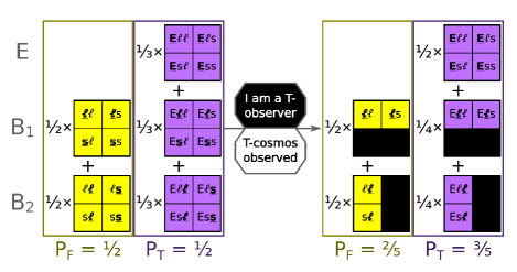
Figure 10: Minimal example of Boltzmann brain problem treated in Weighted FGAI. Both the false and true cosmologies have two Boltzmann observers identical to ourselves; in this case, each with an equal probability of being long-lived ($\ell$) and decaying in a short time ($s$). The true cosmology also has an evolved observer $E$ that always observes it correctly. An observation of T leaves the $E$ provisional physical distribution untouched and also shifts indexical weight to $E$, favoring T.

Our not instantly dissipating is certain if we are evolved observers but unlikely if we are Boltzmann brains. Thus, the indexical weight for any evolved individual location remains $1$, while the indexical weight for any Boltzmann individual location updates to $\eta$. If we are an evolved individual, all microhypotheses survive the observation, while if we are any given Boltzmann individual, only $\eta 2^{N_{B}}$ do. Using equation 10, we now evaluate a posterior credence in cosmology T of:

$$P^{\rm pos}_{T}=\frac{N_{E}+\eta^{2}N_{B_{T}}}{N_{E}+\eta N_{E}+2\eta^{2}N_{B_{T}}}.$$ (12)

As long as $\eta\ll 1$ and $N_{E}\gg\eta^{2}N_{B_{T}}$, we now almost entirely favor cosmology T ($P^{\rm pos}_{T}\approx 1-\eta-\eta^{2}N_{B_{T}}/N_{E}$) (see Figure 10 for a minimal example).

In the above example, we consider only observers with exactly our memories at the start of the observation [as in 6]. There are two reasons this is allowed despite Bostrom [2]’s objections. First, the indexical weights are averaged instead of being defined on the microhypothesis level, and they describe a location reference class instead of an observer reference class. This lets the vast majority of Boltzmann brains that later experience a dissipating universe to influence the final credence: although a given microhypothesis has some locations with long-lived Boltzmann brains, these are no more favored than locations with dissipating Boltzmann brains. Second, unlike the SSA, Weighted FGAI results in an uneven indexical distribution: we place much more weight in each evolved brain location than the Boltzmann brain locations. This actually results in a faster convergence to the realism of the T cosmology than the SSA, requiring only $\eta\ll\sqrt{N_{E}/N_{B_{T}}}$ instead of $N_{E}/N_{B_{T}}$, although this is still nowhere near quickly enough to resolve the Boltzmann brain problem [53].

VI Conclusion

VI.1 Summary of Weighted FGAI

I have developed Weighted FGAI as a framework for interpreting typicality arguments. It shares elements with other frameworks: the auxiliary information about reference classes in Bostrom [2], the use of extremely fine-grained data about observers in Neal [6], and the separately updated indexical distributions of Srednicki and Hartle [32]. It is based on two principles.

The first principle I have argued is that purely indexical facts cannot directly alter physical credence distributions. Indexical facts and physical facts are different types of data, and mixing them together into a joint prior leads to “Presumptuous Philosopher” problems, biasing us towards Large worlds or Small worlds. The difference between indexicals and physical facts is elaborated by different variants of the Sleeping Beauty thought experiment, where the probability refers to different distributions. Yet both types of distributions always exist, even when perfect knowledge about the world or our location in it hides one.

The second principle is that high-level macrotheories about the world can be resolved into a multitude of physically-distinct microhypotheses. The consistency of evidence with each microhypothesis is calculated through physical distributions. In Weighted FGAI, we do not necessarily know which observer we are, so there are provisional physical distributions for every possible trajectory we could be located along in a theory. These are averaged by the indexical weights, summarizing our current beliefs about our location. By defining reference classes by location rather than observer, observations in a large universe can nonetheless be constraining. Although updated separately, they are combined together to form a single physical credence and single indexical distribution for each microhypothesis. Our third-person credence in a macrotheory is then found by summing over all microhypotheses.

I have showed how Weighted FGAI handles several problems involving “typicality”, avoiding fallacious Doomsday Arguments. Several issues remain. First, it is not immune to Bayesian shifts favoring Large theories (for example, constraining observers in non-Earthlike environments without ranking), although it does properly handle some situations where Naive FGAI fails. This alone suggests a still more robust theory of typicality is necessary, perhaps involving revising the priors by trading physical credence with indexical weights (Section V.7). Further issues stem from the need to understand how indexical information is defined and handled. In particular, the indexical weights must be shared between multiple microhypotheses, nominally on the macrotheory level (Section V.5). What exactly counts as indexical information, and what to do when it is ambiguous, may also be problematic. Likewise, it is not entirely clear how to tell when trajectories require separate weights. Finally, the formulation in this paper assumes a finite number of possible observer locations. Nonetheless, it has several desirable properties: it reduces to simple Bayesian updating when either indexical or physical data is fixed, and it can converge to realism faster than the SSA when considering Boltzmann brains.

VI.2 The role of the Copernican Principle in Weighted FGAI

The Copernican insight that we are not unique miracles is deeply ingrained, but not all applications of the idea that “we are typical” are defensible. The parable of the Noonday Argument describes a fallacious application of the principle, demonstrating the problem with the frequentist Doomsday Argument or trying to pick out “special” points of history like its beginning. Other Copernican arguments can have more subtle flaws.

Bayesian typicality arguments rely on $1/N_{\rm total}$ likelihoods: the more possible outcomes there are, the less likely any specific one is observed. Although valid in some circumstances, applying it to rule out Large theories is unacceptable – it can lead to solipsism, in which you are the most typical being because you are the only being. Whereas the Copernican principle motivates us to consider the possibilities of a cosmos where we are living in but one world of many, unrestricted application leads to an epistemic arrogance where you decide your world is the only kind of thing that exists. Yet the mere existence of the environments unlike ours already invalidates the strongest formulations of the Copernican argument: we are either atypical because we are not the only observers that exist, or we live in an atypical place because it contains observers unlike everywhere else in the Universe.

Weighted FGAI is my attempt to deal with how to make inferences in a vast cosmos, and it provides two manifestations of the Copernican Principle. First is an indexical role as a prior, choosing the initial indexical weights by assigning equal weight to each possible position. This role is not trivial because the indexical weights are shared between microhypotheses, which penalizes theories where our location is both rare and random. Yet these indexical weights do not directly affect our credences in physical theories.

The second manifestation of the Copernican Principle is embodied by our physical distributions. Weighted FGAI fine-grains physical theories into microhypotheses describing the exact physical details of every possible outcome. These microhypotheses make no reference to indexical notions like “me” or “us”, only specific physical observers who make specific physical observations at specific physical positions. Observer-relative typicality emerges from the combinatorial properties of these microhypotheses when there is symmetry with respect to position. In other cases, when specific individuals can only exist in certain locations, typicality can fail – this is the anthropic principle at work. Ultimately, the reason why we may often assume ourselves to be typical is because of the uniformity of the physical laws of the cosmos, manifesting both in the symmetry and the panoply of microhypotheses.

Appendix A Explicit urn problem in FGAI

To demonstrate how FGAI can work in practice for most normal kinds of observations, here is an explicit treatment of an urn problem, using a smaller number of participants and balls for compactness.

Say we have two unlabeled urns, $U_{1}$ and $U_{2}$. $U_{1}$ contains one ball, labeled $B_{1}$. $U_{2}$ contains two balls, labeled $B_{1}$ and $B_{2}$. The $B_{1}$ balls in $U_{1}$ and $U_{2}$ are indistinguishable. Four participants in the experiment are each trying to determine whether the urn is $U_{1}$ and $U_{2}$ by drawing a ball (with replacement) and seeing which one it is, but they are not allowed to communicate with each other. The four participants are distinct from each other and named $\alpha$, $\beta$, $\gamma$, and $\delta$, although they may not be aware of it. Each ball in the urn is equally likely to be drawn. All four participants think it equally plausible that the urn is $U_{1}$ or $U_{2}$, so they assign prior credences of $P^{\rm prior}(U_{1})=P^{\rm prior}(U_{2})=1/2$. Suppose $\alpha$ draws $B_{1}$. How should $B_{1}$ update their credences?

If we simply applied the SSA, we would reason that the typical participant draws $B_{1}$ with probability $1$ from $U_{1}$ and $1/2$ from $U_{2}$. Thus their credence in $U_{1}$ should be updated to $P^{\rm pos}(U_{1})=(1\times 1/2)/[(1\times 1/2)+(1/2\times 1/2)]=2/3$.

Table 2: Microhypotheses for urn problem

Urn	$\mu$	Observation model	$P^{\rm prior}$	Observation Likelihoods					$\max{\cal L}(o\to B_{1})$
				$\alpha\to B_{1}$	$o@\textrm{I}\to B_{1}$	$o@\textrm{I}\to B_{2}$	$o@\textrm{I}\to B_{3}$	$o@\textrm{I}\to B_{4}$
1	$B_{1}B_{1}B_{1}B_{1}$	$\begin{array}[]{c}[\{o@\textrm{I},\alpha\}\to B_{1},\{o@\textrm{II},\beta\}\to B_{1},\\ \{o@\textrm{III},\gamma\}\to B_{1},\{o@\textrm{IV},\delta\}\to B_{1}]\end{array}$	$1/2$	1	1	1	1	1	1
2	$B_{1}B_{1}B_{1}B_{1}$	$\begin{array}[]{c}[\{o@\textrm{I},\alpha\}\to B_{1},\{o@\textrm{II},\beta\}\to B_{1},\\ \{o@\textrm{III},\gamma\}\to B_{1},\{o@\textrm{IV},\delta\}\to B_{1}]\end{array}$	$1/32$	1	1	1	1	1	1
	$B_{1}B_{1}B_{1}B_{2}$	$\begin{array}[]{c}[\{o@\textrm{I},\alpha\}\to B_{1},\{o@\textrm{II},\beta\}\to B_{1},\\ \{o@\textrm{III},\gamma\}\to B_{1},\{o@\textrm{IV},\delta\}\to B_{2}]\end{array}$	$1/32$	1	1	1	1	0	1
	$B_{1}B_{1}B_{2}B_{1}$	$\begin{array}[]{c}[\{o@\textrm{I},\alpha\}\to B_{1},\{o@\textrm{II},\beta\}\to B_{1},\\ \{o@\textrm{III},\gamma\}\to B_{2},\{o@\textrm{IV},\delta\}\to B_{1}]\end{array}$	$1/32$	1	1	1	0	1	1
	$B_{1}B_{1}B_{2}B_{2}$	$\begin{array}[]{c}[\{o@\textrm{I},\alpha\}\to B_{1},\{o@\textrm{II},\beta\}\to B_{1},\\ \{o@\textrm{III},\gamma\}\to B_{2},\{o@\textrm{IV},\delta\}\to B_{2}]\end{array}$	$1/32$	1	1	1	0	0	1
	$B_{1}B_{2}B_{1}B_{1}$	$\begin{array}[]{c}[\{o@\textrm{I},\alpha\}\to B_{1},\{o@\textrm{II},\beta\}\to B_{2},\\ \{o@\textrm{III},\gamma\}\to B_{1},\{o@\textrm{IV},\delta\}\to B_{1}]\end{array}$	$1/32$	1	1	0	1	1	1
	$B_{1}B_{2}B_{1}B_{2}$	$\begin{array}[]{c}[\{o@\textrm{I},\alpha\}\to B_{1},\{o@\textrm{II},\beta\}\to B_{2},\\ \{o@\textrm{III},\gamma\}\to B_{1},\{o@\textrm{IV},\delta\}\to B_{2}]\end{array}$	$1/32$	1	1	0	1	0	1
	$B_{1}B_{2}B_{2}B_{1}$	$\begin{array}[]{c}[\{o@\textrm{I},\alpha\}\to B_{1},\{o@\textrm{II},\beta\}\to B_{2},\\ \{o@\textrm{III},\gamma\}\to B_{2},\{o@\textrm{IV},\delta\}\to B_{1}]\end{array}$	$1/32$	1	1	0	0	1	1
	$B_{1}B_{2}B_{2}B_{2}$	$\begin{array}[]{c}[\{o@\textrm{I},\alpha\}\to B_{1},\{o@\textrm{II},\beta\}\to B_{2},\\ \{o@\textrm{III},\gamma\}\to B_{2},\{o@\textrm{IV},\delta\}\to B_{2}]\end{array}$	$1/32$	1	1	0	0	0	1
	$B_{2}B_{1}B_{1}B_{1}$	$\begin{array}[]{c}[\{o@\textrm{I},\alpha\}\to B_{2},\{o@\textrm{II},\beta\}\to B_{1},\\ \{o@\textrm{III},\gamma\}\to B_{1},\{o@\textrm{IV},\delta\}\to B_{1}]\end{array}$	$1/32$	0	0	1	1	1	1
	$B_{2}B_{1}B_{1}B_{2}$	$\begin{array}[]{c}[\{o@\textrm{I},\alpha\}\to B_{2},\{o@\textrm{II},\beta\}\to B_{1},\\ \{o@\textrm{III},\gamma\}\to B_{1},\{o@\textrm{IV},\delta\}\to B_{2}]\end{array}$	$1/32$	0	0	1	1	0	1
	$B_{2}B_{1}B_{2}B_{1}$	$\begin{array}[]{c}[\{o@\textrm{I},\alpha\}\to B_{2},\{o@\textrm{II},\beta\}\to B_{1},\\ \{o@\textrm{III},\gamma\}\to B_{2},\{o@\textrm{IV},\delta\}\to B_{1}]\end{array}$	$1/32$	0	0	1	0	1	1
	$B_{2}B_{1}B_{2}B_{2}$	$\begin{array}[]{c}[\{o@\textrm{I},\alpha\}\to B_{2},\{o@\textrm{II},\beta\}\to B_{1},\\ \{o@\textrm{III},\gamma\}\to B_{2},\{o@\textrm{IV},\delta\}\to B_{2}]\end{array}$	$1/32$	0	0	1	0	0	1
	$B_{2}B_{2}B_{1}B_{1}$	$\begin{array}[]{c}[\{o@\textrm{I},\alpha\}\to B_{2},\{o@\textrm{II},\beta\}\to B_{2},\\ \{o@\textrm{III},\gamma\}\to B_{1},\{o@\textrm{IV},\delta\}\to B_{1}]\end{array}$	$1/32$	0	0	0	1	1	1
	$B_{2}B_{2}B_{1}B_{2}$	$\begin{array}[]{c}[\{o@\textrm{I},\alpha\}\to B_{2},\{o@\textrm{II},\beta\}\to B_{2},\\ \{o@\textrm{III},\gamma\}\to B_{1},\{o@\textrm{IV},\delta\}\to B_{2}]\end{array}$	$1/32$	0	0	0	1	0	1
	$B_{2}B_{2}B_{2}B_{1}$	$\begin{array}[]{c}[\{o@\textrm{I},\alpha\}\to B_{2},\{o@\textrm{II},\beta\}\to B_{2},\\ \{o@\textrm{III},\gamma\}\to B_{2},\{o@\textrm{IV},\delta\}\to B_{1}]\end{array}$	$1/32$	0	0	0	0	1	1
	$B_{2}B_{2}B_{2}B_{2}$	$\begin{array}[]{c}[\{o@\textrm{I},\alpha\}\to B_{2},\{o@\textrm{II},\beta\}\to B_{2},\\ \{o@\textrm{III},\gamma\}\to B_{2},\{o@\textrm{IV},\delta\}\to B_{2}]\end{array}$	$1/32$	0	0	0	0	0	0

In a full FGAI treatment, we list every possible microhypothesis and construct an observation model that lists all possible observations each observer can make, shown in Table 2. Each microhypothesis in this case inherits the same fraction of its parent macrotheory’s weight, determined by the number of microhypotheses in the macrotheory. With four participants, we may assume that there is some indexing (coordinate) system assigning each of $\alpha$, $\beta$, $\gamma$, and $\delta$ to the positions I, II, III, and IV, respectively, perhaps based on the order they make their draws or their proximity to $\alpha$. In this table, a statement of the form $\{o@\textrm{X},\omega\}\to B_{y}$ is shorthand for the propositions that an observer $o$ at position $X$ observes $B_{y}$ as their drawn ball ($o@\textrm{X}\to B_{y}$) and that observer $\omega$ observes $B_{y}$ ($\omega\to B_{y}$) as their drawn ball.

In Weighted FGAI, we need a set of indexical weights, one for each position. The coordinate system described in the setup of the problem places $\alpha$ at position I, and $\alpha$ knows this, so the weights are $(W_{k,\textrm{I}},W_{k,\textrm{II}},W_{k,\textrm{III}},W_{k,\textrm{IV}})=(1,0,0,0)$ in each macrotheory. Knowing they are at position I, they evaluate likelihoods according to the fact that $o@\textrm{I}\to B_{1}$. The normalized weights are never changed. Applying equation 10, $\alpha$ finds $P^{\rm pos}(U_{1})=\{(1\times 3/4)\times[1\times(1\times 1/2)]\}\{(1\times 3/4)\times[1\times(1\times 1/2)]+(1\times 3/4)\times[8\times(1\times 1/32)]\}=2/3$, the correct result. This result is also found in Naive FGAI.

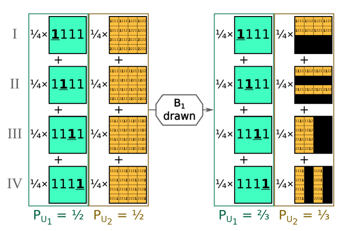
Figure 11: Illustration of the urn example in Weighted FGAI when $\alpha$ does not know their identity, which recovers the expected credences.

But what if $\alpha$ does not know they are $\alpha$, only that they are one of the four participants? Obviously, we can index the participants I, II, III, and IV, but suppose $\alpha$ refuses to work with an implicit indexing system by assigning themself location I and wants to remain agnostic about which “position” they are in? Then $\alpha$ can still proceed with the uninformative, SSA indexical weights $(w_{k,\textrm{I}},w_{k,\textrm{II}},w_{k,\textrm{III}},w_{k,\textrm{IV}})=(1,1,1,1)$. Upon drawing a heads, the indexical weights remain uninformative. Applying equation 10, $\alpha$ finds $P^{\rm pos}(U_{1})=\{(4\times 3/4)\times[1\times(1\times 1/2)]\}/\{(4\times 3/4)\times[1\times(1\times 1/2)]+(4\times 3/4)\times[8\times(1\times 1/32)]\}=\frac{2}{3}$. Figure 11 illustrates how the provisional physical distributions for the microhypotheses update. The same result is found in Naive FGAI.

Note that if every single microhypothesis got its own set of indexical weights, updated by each observation, then the weights of each would shift to accommodate the $B_{1}$ observation. As in the strictest interpretation of Naive FGAI, the derived $P^{\rm pos}(U_{1})$ would then be $16/31$.

Appendix B Explicit Doomsday problem in Weighted FGAI

In this section, I work out an explicit example of a Doomsday-type problem in Weighted FGAI. Although extremely simple, it nonetheless illustrates several points: Doomsday failing for internal observers while working for an external observer, how to handle multiple “worlds” of humanity, and how to treat hierarchical models in USO with unequal prior credence in the microhypotheses.

The model consists of two “worlds”, indexed I and II based on some otherwise unknown distinction. Each world contains a short sequence of human observers. In the Small model, $N_{\rm total}=1$ for both, while in the Large model, $N_{\rm total}=2$ for both. These humans are drawn from two subsets, $H_{a}=\{A_{a}\}$ and $H_{b}=\{A_{b},B_{b}\}$, of unequal size. This is a USO model: due to unknown historical contingencies, $H_{a}$ humans can only be born at one of birthrank $1$ or $2$ which is the same for all worlds, and likewise for $H_{b}$. In addition, an external alien observer $X$ who knows all this deliberately seeks out humanity, arriving at one of the two worlds, but not knowing which or what time beforehand. Each human observes which member of $H\equiv H_{a}\cup H_{b}$ they are and measures their birthrank accurately, but cannot observe humans at other birthranks or in the partner world. Likewise, if $X$ is present at that world and that time, they measure which human is present and what their birthrank is.

The microhypotheses in this problem are listed in Table 3. These microhypotheses indicate the birthrank order of $H_{a}$ and $H_{b}$, the exact sequence of each world, and the human observed by $X$, denoted by $Y^{\text{\char 53}}$. The arrival of $X$ is a physical event and thus different locations of $X$ are properly treated as physical microhypotheses. This example is somewhat complicated because $H_{a}$ and $H_{b}$ are different size. Thus permutations with only $H_{b}$ are more numerous than those with $H_{a}$. The correct approach is to regard the ordering of $a$ and $b$ as intermediate-level parameters: it is just as likely that $H_{a}$ has rank 1 as $H_{b}$ has rank 1. Thus Small microhypotheses with only $b$ humans have lower prior weight $P^{\rm prior}$ than those with only $a$ humans for a balanced credence. In the Table, quantities referring to World I and World II are separated by a vertical bar, while quantities referring to humans at different birthranks within a world are separated by a comma.

Table 3: Microhypotheses for two-world USO Doomsday problem

$N_{\rm total}$	Order	$\mu$	$P^{\rm prior}$	Human observation likelihoods				External observation likelihoods
				$o=A_{a}$	$o=A_{a}@1$	$o=A_{b}$	$o=A_{b}@1$	$A_{a}$	$A_{a}@1$	$A_{b}$	$A_{b}@1$
$1$	$a$	$A_{a}^{\text{\char 53}}|A_{a}$	$1/8$	$(1|1)$	$(1|1)$	$(0|0)$	$(0|0)$	$1$	$1$	$0$	$0$
		$A_{a}|A_{a}^{\text{\char 53}}$	$1/8$	$(1|1)$	$(1|1)$	$(0|0)$	$(0|0)$	$1$	$1$	$0$	$0$
	$b$	$A_{b}^{\text{\char 53}}|A_{b}$	$1/32$	$(0|0)$	$(0|0)$	$(1|1)$	$(1|1)$	$0$	$0$	$1$	$1$
		$A_{b}|A_{b}^{\text{\char 53}}$	$1/32$	$(0|0)$	$(0|0)$	$(1|1)$	$(1|1)$	$0$	$0$	$1$	$1$
		$A_{b}^{\text{\char 53}}|B_{b}$	$1/32$	$(0|0)$	$(0|0)$	$(1|0)$	$(1|0)$	$0$	$0$	$1$	$1$
		$A_{b}|B_{b}^{\text{\char 53}}$	$1/32$	$(0|0)$	$(0|0)$	$(1|0)$	$(1|0)$	$0$	$0$	$0$	$0$
		$B_{b}^{\text{\char 53}}|A_{b}$	$1/32$	$(0|0)$	$(0|0)$	$(0|1)$	$(0|1)$	$0$	$0$	$0$	$0$
		$B_{b}|A_{b}^{\text{\char 53}}$	$1/32$	$(0|0)$	$(0|0)$	$(0|1)$	$(0|1)$	$0$	$0$	$1$	$1$
		$B_{b}^{\text{\char 53}}|B_{b}$	$1/32$	$(0|0)$	$(0|0)$	$(0|0)$	$(0|0)$	$0$	$0$	$0$	$0$
		$B_{b}|B_{b}^{\text{\char 53}}$	$1/32$	$(0|0)$	$(0|0)$	$(0|0)$	$(0|0)$	$0$	$0$	$0$	$0$
$2$	$ab$	$A_{a}^{\text{\char 53}},A_{b}|A_{a},A_{b}$	$1/64$	$(1,0|1,0)$	$(1,0|1,0)$	$(0,1|0,1)$	$(0,0|0,0)$	$1$	$1$	$0$	$0$
		$A_{a},A_{b}^{\text{\char 53}}|A_{a},A_{b}$	$1/64$	$(1,0|1,0)$	$(1,0|1,0)$	$(0,1|0,1)$	$(0,0|0,0)$	$0$	$0$	$1$	$0$
		$A_{a},A_{b}|A_{a}^{\text{\char 53}},A_{b}$	$1/64$	$(1,0|1,0)$	$(1,0|1,0)$	$(0,1|0,1)$	$(0,0|0,0)$	$1$	$1$	$0$	$0$
		$A_{a},A_{b}|A_{a},A_{b}^{\text{\char 53}}$	$1/64$	$(1,0|1,0)$	$(1,0|1,0)$	$(0,1|0,1)$	$(0,0|0,0)$	$0$	$0$	$1$	$0$
		$A_{a}^{\text{\char 53}},A_{b}|A_{a},B_{b}$	$1/64$	$(1,0|1,0)$	$(1,0|1,0)$	$(0,1|0,0)$	$(0,0|0,0)$	$1$	$1$	$0$	$0$
		$A_{a},A_{b}^{\text{\char 53}}|A_{a},B_{b}$	$1/64$	$(1,0|1,0)$	$(1,0|1,0)$	$(0,1|0,0)$	$(0,0|0,0)$	$0$	$0$	$1$	$0$
		$A_{a},A_{b}|A_{a}^{\text{\char 53}},B_{b}$	$1/64$	$(1,0|1,0)$	$(1,0|1,0)$	$(0,1|0,0)$	$(0,0|0,0)$	$1$	$1$	$0$	$0$
		$A_{a},A_{b}|A_{a},B_{b}^{\text{\char 53}}$	$1/64$	$(1,0|1,0)$	$(1,0|1,0)$	$(0,1|0,0)$	$(0,0|0,0)$	$0$	$0$	$0$	$0$
		$A_{a}^{\text{\char 53}},B_{b}|A_{a},A_{b}$	$1/64$	$(1,0|1,0)$	$(1,0|1,0)$	$(0,0|0,1)$	$(0,0|0,0)$	$1$	$1$	$0$	$0$
		$A_{a},B_{b}^{\text{\char 53}}|A_{a},A_{b}$	$1/64$	$(1,0|1,0)$	$(1,0|1,0)$	$(0,0|0,1)$	$(0,0|0,0)$	$0$	$0$	$0$	$0$
		$A_{a},B_{b}|A_{a}^{\text{\char 53}},A_{b}$	$1/64$	$(1,0|1,0)$	$(1,0|1,0)$	$(0,0|0,1)$	$(0,0|0,0)$	$1$	$1$	$0$	$0$
		$A_{a},B_{b}|A_{a},A_{b}^{\text{\char 53}}$	$1/64$	$(1,0|1,0)$	$(1,0|1,0)$	$(0,0|0,1)$	$(0,0|0,0)$	$0$	$0$	$1$	$0$
		$A_{a}^{\text{\char 53}},B_{b}|A_{a},B_{b}$	$1/64$	$(1,0|1,0)$	$(1,0|1,0)$	$(0,0|0,0)$	$(0,0|0,0)$	$1$	$1$	$0$	$0$
		$A_{a},B_{b}^{\text{\char 53}}|A_{a},B_{b}$	$1/64$	$(1,0|1,0)$	$(1,0|1,0)$	$(0,0|0,0)$	$(0,0|0,0)$	$0$	$0$	$0$	$0$
		$A_{a},B_{b}|A_{a}^{\text{\char 53}},B_{b}$	$1/64$	$(1,0|1,0)$	$(1,0|1,0)$	$(0,0|0,0)$	$(0,0|0,0)$	$1$	$1$	$0$	$0$
		$A_{a},B_{b}|A_{a},B_{b}^{\text{\char 53}}$	$1/64$	$(1,0|1,0)$	$(1,0|1,0)$	$(0,0|0,0)$	$(0,0|0,0)$	$0$	$0$	$0$	$0$
	$ba$	$A_{b}^{\text{\char 53}},A_{a}|A_{b},A_{a}$	$1/64$	$(0,1|0,1)$	$(0,0|0,0)$	$(1,0|1,0)$	$(1,0|1,0)$	$0$	$0$	$1$	$1$
		$A_{b},A_{a}^{\text{\char 53}}|A_{b},A_{a}$	$1/64$	$(0,1|0,1)$	$(0,0|0,0)$	$(1,0|1,0)$	$(1,0|1,0)$	$1$	$0$	$0$	$0$
		$A_{b},A_{a}|A_{b}^{\text{\char 53}},A_{a}$	$1/64$	$(0,1|0,1)$	$(0,0|0,0)$	$(1,0|1,0)$	$(1,0|1,0)$	$0$	$0$	$1$	$1$
		$A_{b},A_{a}|A_{b},A_{a}^{\text{\char 53}}$	$1/64$	$(0,1|0,1)$	$(0,0|0,0)$	$(1,0|1,0)$	$(1,0|1,0)$	$1$	$0$	$0$	$0$
		$A_{b}^{\text{\char 53}},A_{a}|B_{b},A_{a}$	$1/64$	$(0,1|0,1)$	$(0,0|0,0)$	$(1,0|0,0)$	$(1,0|0,0)$	$0$	$0$	$1$	$1$
		$A_{b},A_{a}^{\text{\char 53}}|B_{b},A_{a}$	$1/64$	$(0,1|0,1)$	$(0,0|0,0)$	$(1,0|0,0)$	$(1,0|0,0)$	$1$	$0$	$0$	$0$
		$A_{b},A_{a}|B_{b}^{\text{\char 53}},A_{a}$	$1/64$	$(0,1|0,1)$	$(0,0|0,0)$	$(1,0|0,0)$	$(1,0|0,0)$	$0$	$0$	$0$	$0$
		$A_{b},A_{a}|B_{b},A_{a}^{\text{\char 53}}$	$1/64$	$(0,1|0,1)$	$(0,0|0,0)$	$(1,0|0,0)$	$(1,0|0,0)$	$1$	$0$	$0$	$0$
		$B_{b}^{\text{\char 53}},A_{a}|A_{b},A_{a}$	$1/64$	$(0,1|0,1)$	$(0,0|0,0)$	$(0,0|1,0)$	$(0,0|1,0)$	$0$	$0$	$0$	$0$
		$B_{b},A_{a}^{\text{\char 53}}|A_{b},A_{a}$	$1/64$	$(0,1|0,1)$	$(0,0|0,0)$	$(0,0|1,0)$	$(0,0|1,0)$	$1$	$0$	$0$	$0$
		$B_{b},A_{a}|A_{b}^{\text{\char 53}},A_{a}$	$1/64$	$(0,1|0,1)$	$(0,0|0,0)$	$(0,0|1,0)$	$(0,0|1,0)$	$0$	$0$	$1$	$1$
		$B_{b},A_{a}|A_{b},A_{a}^{\text{\char 53}}$	$1/64$	$(0,1|0,1)$	$(0,0|0,0)$	$(0,0|1,0)$	$(0,0|1,0)$	$1$	$0$	$0$	$0$
		$B_{b}^{\text{\char 53}},A_{a}|B_{b},A_{a}$	$1/64$	$(0,1|0,1)$	$(0,0|0,0)$	$(0,0|0,0)$	$(0,0|0,0)$	$0$	$0$	$0$	$0$
		$B_{b},A_{a}^{\text{\char 53}}|B_{b},A_{a}$	$1/64$	$(0,1|0,1)$	$(0,0|0,0)$	$(0,0|0,0)$	$(0,0|0,0)$	$1$	$0$	$0$	$0$
		$B_{b},A_{a}|B_{b}^{\text{\char 53}},A_{a}$	$1/64$	$(0,1|0,1)$	$(0,0|0,0)$	$(0,0|0,0)$	$(0,0|0,0)$	$0$	$0$	$0$	$0$
		$B_{b},A_{a}|B_{b},A_{a}^{\text{\char 53}}$	$1/64$	$(0,1|0,1)$	$(0,0|0,0)$	$(0,0|0,0)$	$(0,0|0,0)$	$1$	$0$	$0$	$0$

Internal observers – You are a human and you have worked out this model exactly. You wish to use a Doomsday Argument by determining which human in $H$ you are and also your birthrank. To do this in Weighted FGAI, you require indexical weights for the Small and Large theories. Since you know you are human and not the alien, you use the initial indexical weight vector $(w_{L,\mathrm{I},1},w_{L,\mathrm{1},2}|w_{L,\mathrm{II},1},w_{L,\mathrm{II},2})=(1,1|1,1)$ in the Long theory and $(w_{S,\mathrm{I},1}|w_{S,\mathrm{II},1})=(1|1)$ in the Short theory. Columns 5–8 give likelihoods that a human at each position will make a given observation.

Now suppose you observe that you are $A_{a}$. Half of all microhypotheses are consistent with each position, so the indexical weights update to $(1/2,1/2|1/2,1/2)$ for the Long theory and $(1/2|1/2)$ for the Short theory. The credence in the Small theory updates to $(1/2\times 2/8+1/2\times 2/8)/[(1/2\times 2/8+1/2\times 2/8)+(1/4\times 16/64+1/4\times 16/64+1/4\times 16/64+1/4\times 16/64)]=1/2$ – unchanged from before. Next, you happen to measure your birthrank to be $1$. In all microhypotheses in both theories, this is only consistent with having a birthrank of $1$, prompting an update of the indexical weights to $(1/2,0|1/2,0)$ in Long. Using the likelihoods in the Table, the credence in the Small theory updates to $(1/2\times 2/8+1/2\times 2/8)/[(1/2\times 2/8+1/2\times 2/8)+(1/2\times 16/64+1/2\times 16/64)]=1/2$. The Doomsday Argument has failed for $A_{a}$ because of the shifting indexical weights (Figure 12).

The Doomsday Argument also fails for $A_{b}$ (and $B_{b}$ by symmetry) if they attempt it. Upon discovering they are $A_{b}$, each $w_{k,i}$ updates to $1/4$ and the credence in the Small theory remains unchanged: $(1/2\times 4/32+1/2\times 4/32)/[(1/2\times 4/32+1/2\times 4/32)+(1/4\times 8/64+1/4\times 8/64+1/4\times 8/64+1/4\times 8/64)]=1/2$. If $A_{b}$ finds themself at birthrank 1, the Large theory indexical weights again shift to $(1/4,0|1/4,0)$ in Long, and the credence in the Small theory is $(1/2\times 4/32+1/2\times 4/32)/[(1/2\times 4/32+1/2\times 4/32)+(1/2\times 8/64+1/2\times 8/64)]=1/2$.

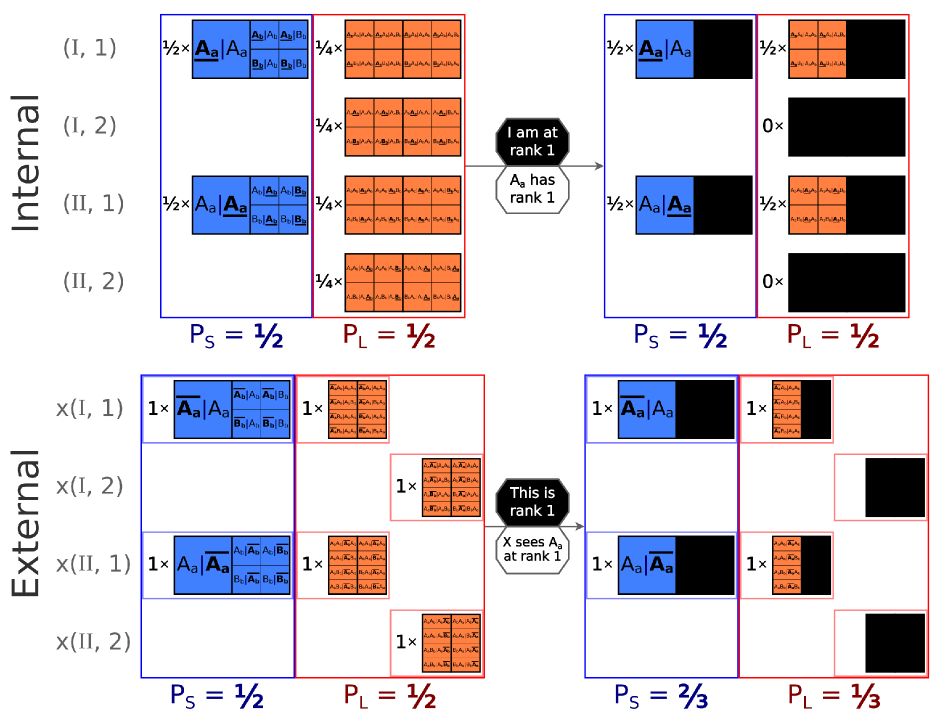
Figure 12: Illustration of the Doomsday Argument example in Weighted FGAI when $A_{a}$ is observed at rank $1$ by $A_{a}$ themself or by an external observer. The observed human is bold, with an underline for a self-observation and an overline for an external observation. The distinctions about $X$’s position are ignored in the Internal case, where each microhypothesis stands for four from Table 3.

External observers – You are the alien observer and you have worked out this model exactly. You wish to use a Doomsday Argument based on your observations of who is currently living and their birthrank. You are the only external observer, although there are four possible locations: $\mathrm{x}(\textrm{I},1)$, $\mathrm{x}(\textrm{I},2)$, $\mathrm{x}(\textrm{II},1)$, and $\mathrm{x}(\textrm{II},2)$ (Figure 12). The different possible locations of $X$ – a physical distinction – also correspond to different groups of microhypotheses, each with only one valid indexical weight (Figure 12). Because $X$’s position has no effect on the sequence of humans, there is a complete symmetry in the prior provisional credences between all microhypotheses. Columns 9–12 give likelihoods for the observations you may make.

Suppose you observe $A_{a}$ from $H_{a}$. This does not by itself affect your credence in the Small theory: $(2\times 1\times 1/8)/[(2\times 1\times 1/8)+(4\times 1\times 1/16)]=1/2$. But if you measure $A_{a}$’s birthrank to be $1$, that credence updates to $(2\times 1\times 1/8)/[(2\times 1\times 1/8)+(2\times 1\times 1/16)]=2/3$. The same results are found if you observe $A_{b}$ at rank $1$: first, a Small credence of $(2\times 1\times 1/16)/[(2\times 1\times 1/16)+(4\times 1\times 1/32)]=1/2$ when you observe $A_{b}$, then $(2\times 1\times 1/16)/[(2\times 1\times 1/16)+(2\times 1\times 1/32)]=2/3$. For you, the Doomsday Argument is validated by Weighted FGAI.

The difference results from two factors. First, there is an extra temporal degree of freedom for $X$’s arrival. Second, $X$’s position is entirely fixed in each microhypothesis – knowing they are the external observer, $X$ can predict exactly who they will observe simply based on time of arrival, since the time of arrival is entirely a physical statement. In contrast, there is no single “time of observation” for the humans in Large model, since one observes early and one observes late. For the internal case, all microhypotheses are present in the Long provisional physical distributions, because there are observers at all locations. A priori, the internal observer places equal provisional prior credence in the Short and Long theories for the rank $1$ positions. But in the external case, the rank $1$ and rank $2$ positions constrain completely different Long microhypotheses, splitting the Long prior credence between them. A priori, the external observer places twice as much provisional prior credence in Short than Long for the rank $1$ positions. This is illustrated in Figure 12.

References

- Leslie [1996] J. Leslie, The end of the world: the science and ethics of human extinction (Routledge, 1996).
- Bostrom [2013] N. Bostrom, Anthropic bias: Observation selection effects in science and philosophy (Routledge, 2013).
- Carter [1974] B. Carter, in Confrontation of Cosmological Theories with Observational Data, Vol. 63, edited by M. S. Longair (1974) pp. 291–298.
- Carter [1983] B. Carter, Philosophical Transactions of the Royal Society of London Series A 310, 347 (1983).
- Barrow [1983] J. D. Barrow, Quarterly Journal of the Royal Astronomical Society 24, 146 (1983).
- Neal [2006] R. M. Neal, arXiv Mathematics e-prints , math/0608592 (2006), arXiv:math/0608592 [math.ST] .
- Garriga and Vilenkin [2008] J. Garriga and A. Vilenkin, Physical Review D 77, 043526 (2008), arXiv:0711.2559 [hep-th] .
- Bostrom [2002] N. Bostrom, The Journal of philosophy 99, 607 (2002).
- Bousso et al. [2008] R. Bousso, B. Freivogel, and I. S. Yang, Physical Review D 77, 103514 (2008), arXiv:0712.3324 [hep-th] .
- Vilenkin [1995] A. Vilenkin, Phys. Rev. Lett. 74, 846 (1995), arXiv:gr-qc/9406010 [gr-qc] .
- Gott [1993] I. Gott, J. R., Nature 363, 315 (1993).
- Nielsen [1989] H. B. Nielsen, Acta Physica Polonica, Series B 20, 427 (1989).
- Knobe et al. [2006] J. Knobe, K. D. Olum, and A. Vilenkin, The British journal for the philosophy of science 57, 47 (2006), arXiv:physics/0302071 .
- Olum [2003] K. D. Olum, arXiv e-prints , gr-qc/0303070 (2003), arXiv:gr-qc/0303070 [gr-qc] .
- Tarter [2001] J. Tarter, Annual Review of Astronomy and Astrophysics 39, 511 (2001).
- Bracewell [1960] R. N. Bracewell, Nature 186, 670 (1960).
- Sagan [1973] C. Sagan, Icarus 19, 350 (1973).
- Forgan and Nichol [2011] D. H. Forgan and R. C. Nichol, International Journal of Astrobiology 10, 77 (2011), arXiv:1007.0850 [astro-ph.EP] .
- Dyson [1960] F. J. Dyson, Science 131, 1667 (1960).
- Kardashev [1964] N. S. Kardashev, Soviet Astronomy 8, 217 (1964).
- Bostrom [2003] N. Bostrom, Utilitas 15, 308 (2003).
- Cirkovic [2004] M. M. Cirkovic, Foundations of Physics 34, 239 (2004), arXiv:astro-ph/0211414 [astro-ph] .
- Bostrom [2001] N. Bostrom, Synthese 127, 359 (2001).
- Dieks [1992] D. Dieks, The Philosophical Quarterly (1950-) 42, 78 (1992).
- Kopf et al. [1994] T. Kopf, P. Krtous, and D. N. Page, arXiv e-prints , gr-qc/9407002 (1994), arXiv:gr-qc/9407002 [gr-qc] .
- Korb and Oliver [1998] K. B. Korb and J. J. Oliver, Mind 107, 403 (1998).
- Monton and Roush [2001] B. Monton and S. Roush, Gott’s doomsday argument (2001).
- Olum [2002] K. D. Olum, The Philosophical Quarterly 52, 164 (2002).
- Benétreau-Dupin [2015] Y. Benétreau-Dupin, Philosophy of Science 82, 879 (2015), 1412.4382 .
- Garisto [2020] R. Garisto, Physical Review Research 2, 033464 (2020).
- Friederich [2017] S. Friederich, Physical Review D 95, 123520 (2017), arXiv:1707.04419 [physics.hist-ph] .
- Srednicki and Hartle [2010] M. Srednicki and J. Hartle, Physical Review D 81, 123524 (2010), arXiv:0906.0042 [hep-th] .
- Cirkovic [2001] M. M. Cirkovic, arXiv e-prints , gr-qc/0110002 (2001), arXiv:gr-qc/0110002 [gr-qc] .
- Bostrom and Ćirković [2003] N. Bostrom and M. M. Ćirković, The Philosophical Quarterly 53, 83 (2003).
- Haqq-Misra et al. [2018] J. Haqq-Misra, R. K. Kopparapu, and E. T. Wolf, International Journal of Astrobiology 17, 77 (2018), arXiv:1705.07813 [physics.pop-ph] .
- Dayal et al. [2015] P. Dayal, C. Cockell, K. Rice, and A. Mazumdar, Astrophysical Journal Letters 810, L2 (2015), arXiv:1507.04346 [astro-ph.GA] .
- Whitmire [2020] D. P. Whitmire, Monthly Notices of the Royal Astronomical Society 494, 3048 (2020), arXiv:2003.13643 [astro-ph.EP] .
- Kaneda and Haub [2020] T. Kaneda and C. Haub, How many people have ever lived on earth (2020).
- Jefferys and Berger [1991] W. H. Jefferys and J. O. Berger, Sharpening Ockham’s razor on a Bayesian strop (1991).
- Hartle and Srednicki [2007] J. B. Hartle and M. Srednicki, Physical Review D 75, 123523 (2007), arXiv:0704.2630 [hep-th] .
- Leslie [1994] J. Leslie, Journal of applied philosophy 11, 31 (1994).
- Crowe [1999] M. J. Crowe, The Extraterrestrial Life Debate 1750-1900: The idea of a plurality of worlds from Kant to Lowell (Dover Publications, 1999).
- Griffin and Speck [2004] D. R. Griffin and G. B. Speck, Animal cognition 7, 5 (2004).
- Chalmers [1996] D. J. Chalmers, The conscious mind: In search of a fundamental theory (Oxford University Press, 1996) pp. 94–99.
- Elga [2000] A. Elga, Analysis 60, 143 (2000).
- Bostrom [2007] N. Bostrom, Synthese 157, 59 (2007).
- Laplace [1902] P. S. Laplace, A philosophical essay on probabilities (1902).
- Bostrom [2003] N. Bostrom, The Philosophical Quarterly 53, 243 (2003).
- Gott [1997] J. R. Gott, New Scientist , 36 (1997).
- Adams and Laughlin [1997] F. C. Adams and G. Laughlin, Reviews of Modern Physics 69, 337 (1997), arXiv:astro-ph/9701131 [astro-ph] .
- Bousso [2002] R. Bousso, Reviews of Modern Physics 74, 825 (2002), arXiv:hep-th/0203101 [hep-th] .
- Ćirković et al. [2010] M. M. Ćirković, A. Sandberg, and N. Bostrom, Risk Analysis: An International Journal 30, 1495 (2010).
- Dyson et al. [2002] L. Dyson, M. Kleban, and L. Susskind, Journal of High Energy Physics 2002, 011 (2002), arXiv:hep-th/0208013 [hep-th] .
- Albrecht and Sorbo [2004] A. Albrecht and L. Sorbo, Physical Review D 70, 063528 (2004), arXiv:hep-th/0405270 [hep-th] .
- Carroll [2017] S. M. Carroll, arXiv e-prints , arXiv:1702.00850 (2017), arXiv:1702.00850 [hep-th] .
- DeRosset [2009] L. DeRosset, Philosophy Compass 4, 998 (2009).
- Freivogel [2011] B. Freivogel, Classical and Quantum Gravity 28, 204007 (2011), arXiv:1105.0244 [hep-th] .