Learning Deep Morphological Networks with Neural Architecture Search

Abstract

Deep Neural Networks (DNNs) are generated by sequentially performing linear and non-linear processes. The combination of linear and non-linear procedures is critical for generating a sufficiently deep feature space. Most non-linear operators are derivations of activation functions or pooling functions. Mathematical morphology is a branch of mathematics that provides non-linear operators for various image processing problems. This paper investigates the utility of integrating these operations into an end-to-end deep learning framework. DNNs are designed to acquire a realistic representation for a particular job. Morphological operators give topological descriptors that convey salient information about the shapes of objects depicted in images. We propose a method based on meta-learning to incorporate morphological operators into DNNs. The learned architecture demonstrates how our novel morphological operations significantly increase DNN performance on various tasks, including picture classification, edge detection, and semantic segmentation. Our codes are available at https://nao-morpho.github.io/.

Keywords Mathematical morphology; deep learning; architecture search; edge detection; semantic segmentation.

1 Introduction

Over the last decade, deep learning has made several breakthroughs and demonstrated successful applications in various fields (e.g. computer vision Krizhevsky et al. (2012); Simonyan and Zisserman (2014a); He et al. (2016), object detection Redmon et al. (2016), and NLP Radford et al. (2019)). This success is mainly attributable to the fact that the feature engineering process is automated, whereby features are learned in an end-to-end process from data rather than designed manually. The need for improved architecture has swiftly followed the advent of deep learning, with experts now placing a premium on architecture engineering in lieu of feature engineering.

Architecture engineering is concerned with determining the most appropriate operations for a network, their hyper-parameters (e.g. the number of neurons for fully connected layers or the number of filters or the kernel size for convolutional layers), and the connectivity of all operations. Generally, practitioners propose novel operations to validate various architectures and tasks to improve performance on specific tasks. As a result, developing a novel operation remains a time-consuming and costly process that necessitates a manual search for the optimal configuration. It is, therefore, prone to failure when practitioners lack computational resources. An alternative approach focuses on automatically finding the network architecture design using Neural Architecture Search (NAS) methods Liu et al. (2019a); Luo et al. (2019); Liu et al. (2018); Pham et al. (2018); Weng et al. (2019) in lieu of manual design. Given a set of data and a performance metric for a learning task, an NAS algorithm attempts to find the optimal architecture for a search strategy. It can be viewed as an optimization problem in the space of an architecture network defined by a collection of operations and their possible combinations. Recently, it was demonstrated empirically on several applications that architectures discovered using NAS outperform those discovered manually.

We are observing steadily increasing interest in mathematical morphology among the deep learning community. Indeed, the intrinsic features of mathematical morphology operators that enable them to extract information from topological structures make them excellent candidates. Morphological operators have been shown to capture image edges Rivest et al. (1993), granulometry Serra (1988); Thibault et al. (2013), and distances to object borders Franchi and Angulo (2014). The literature primarily employs two methodologies to evaluate the utility of morphological operators. Some analyses  Cavallaro et al. (2017); Velasco-Forero and Angulo (2013); Franchi and Angulo (2016) directly extract descriptors from unlearned morphological layers, while others  Franchi et al. (2020); Valle (2020); Mondal et al. (2020) propose learning the structural element of the morphological operators. Despite their superior performance in various applications, these methodologies are prone to failure if the deep network architecture is misdesigned, which may dissuade researchers from pursuing this research path.

This paper proposes a novel methodology based on NAS to assess the usefulness of newly developed architecture layers and, in particular, morphological layers (see Figure 1). The following empirically investigates morphological layers applied to deep networks on CIFAR10/CIFAR100 Krizhevsky (2009) an edge detection task using BSD500 Martin et al. (2001), and a semantic segmentation task on Cityscapes Cordts et al. (2016) to determine the optimal design for morphological layers. We perform a comparison between our results and the best architecture discovered using conventional convolutional layers.

Our contributions can be summarized as follows:

• First, we propose novel procedures based on sub-pixel convolutions and mathematical morphology to construct pseudo morphological operations using standard convolution layers.

• We integrate these procedures into deep networks using morphological layers and NAS algorithms. We demonstrate empirically that our architecture tailored to morphological layers can outperform conventional convolutional layers.

• We outline some current issues in NAS and introduce the problem of choosing the backbone, i.e. the higher-level architecture design on which the search will be performed. We offer novel network space descriptions suitable for the edge identification task.

• We are the first to examine architectural search mixed with morphological procedures for edge detection and semantic segmentation. Our new specialized architecture achieves state-of-the-art performance in edge detection.

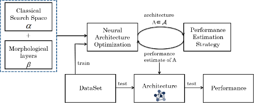
Figure 1: The overall methodology based on neural architecture search to assess the usefulness of morphological layers.

2 Related work

2.1 Mathematical Morphology

Mathematical morphology has been extensively used to denoise raw images Serra (1983); Bouchet et al. (2016) as well as characterize and analyze microscopic images Franchi et al. (2018) and remote sensing images Franchi and Angulo (2016, 2014); Cavallaro (2016); Cavallaro et al. (2017); Velasco-Forero and Angulo (2013). Additionally, these operators have been employed to generate medical images Dufour et al. (2013); Zhang et al. (2012). However, all of these morphological paper operators were used as filters to derive feature descriptors from the classifier’s input data. Here, we integrate them into a DNN.

2.2 Morphological Neural Network

Masci et al.Masci et al. (2013) pioneered the use of morphological operators in neural networks by researching pseudo harmonic morphological operators in conjunction with DNNs. The first morphological Perceptrons were investigated in Saeedan et al. (2018); Mondal et al. (2019); Valle (2020); Charisopoulos and Maragos (2017). Some investigations attempted to integrate morphological layers and DNN architecture Mellouli et al. (2017); Mondal et al. (2020); Franchi et al. (2020); Nogueira et al. (2019). The issue with these works is that the effectiveness of morphological layers are arguably architecture-dependent, and hence, our work proposes linking the search for architecture using morphological layers. We hereby disregard the work of Blusseau et al. Blusseau et al. (01 Jan. 2020), who used auto-encoder networks to approximate morphological operators.

2.3 Neural Architecture Search

Experts in the machine learning field typically create DNNs by hand and select hyper-parameters through trial-and-error, making the process tiring and tedious as well as prone to errors. A different perspective sees model design as a decision-making process that can be improved wherein we can automatically find the best combination of algorithms to maximize the performance of a task. Amidst the growing interest in deep learning, AutoML Zöller and Huber (2019) and NAS Liu et al. (2018) have emerged, whereby the entire DL pipeline can be automated, aiming to reduce the overall development cost and approach expert performance. There have been several efforts Pham et al. (2018); Luo et al. (2019), as early as the 1990s Kitano (1990), to formulate NAS as an optimization in the space of network architectures, solved using either reinforcement learning algorithms Pham et al. (2018), gradient-based optimization Liu et al. (2019a), sequential model-based optimization Luo et al. (2019); Camero et al. (2020), or evolutionary algorithms Liu et al. (2021); Loshchilov and Hutter (2016). While several search strategies have been investigated, gradient-based and sequential-based methods appear to reach state-of-the-art performance with lower computational cost Ren et al. (2020). Despite good performance, agent-based methods Zoph et al. (2018) and evolutionary algorithms remain expensive as they require time and effort to reach a good candidate solution Song et al. (2021). Moreover, as explained in Eiben and Smit (2011), evolutionary algorithms are highly sensitive to the hyperparameters. Here, we use NAO Luo et al. (2019), which is a good compromise.

3 Morphological Architecture Search (MAS)

We first outline some preliminaries on the convolution operation and its relationship to mathematical morphology in Sec. 3.1. We then outline our proposed pseudo morphological dilation operation (Sec. 3.2) and its variants (Sec. 3.3). Next, we explain the architecture search algorithm that we use to integrate the operators into a neural network (Sec. 3.4). Finally, we describe the proposed architecture backbone.

3.1 Preliminaries

Consider a discrete RGB image $f$, where $f[i,j,0],f[i,j,1],f[i,j,2]$ denote the red, green, and blue values at position $(i,j)$, respectively. We further denote $g$ as the feature map resulting from a DNN’s convolution layer of $f$ with the filter $\omega$ without bias. The feature map $g$ can be expressed as:

$$g[n_{1},n_{2},c]=\sum_{k=0}^{2}\sum_{(i,j)\in\mathcal{N}}f[n_{1}+i,n_{2}+j,k]\omega[i,j,k]+b[c]\mbox{ , with }c\in[1,C_{\mbox{out}}]$$ (1)

where $\mathcal{N}$ is a square kernel that defines the spatial size of the convolution kernel, $c$ is the index of the channel, $C_{\mbox{out}}$ is the number of channels output by the layer, and $b$ is the bias, which is equal to zero if we consider unbiased convolution.

By analogy, mathematical morphology Serra (1983) operators are non-linear image operators based on the spatial structure of the image. Initially, these operators were proposed for binary images, but have now been extended to grayscale images. Let $f$ be a grayscale image representing a function, with the intensity at position $x$ denoted as $f(x)$. The two basic operations in morphology are performed at the gray level, such that we define the erosion and dilation operations on their discrete version respectively as: $\varepsilon_{b}(f)[n_{1},n_{2}]=\min_{(i,j)\in\mathcal{N}}f[n_{1}+i,n_{2}+j]-b[i,j]$ and $\varepsilon_{b}(f)[n_{1},n_{2}]=\max_{(i,j)\in\mathcal{N}}f[n_{1}-i,n_{2}-j]+b[i,j]$, where $b=\left[b_{-n},\ldots,b_{n}\right]$ is a structuring element (SE). In Figure 2, we observe that the dilation increases the bright areas based on the shape of the SE, leading to a brighter image. Erosion is the morphological dual to dilation and decreases the bright areas. We can see a direct link between the dilation/erosion and convolution, whereby the dilation is a convolution in the max + algebra, as explained in Angulo (2017).

(a)

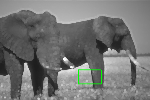
(b)

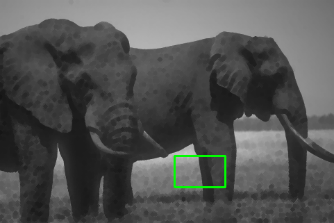
(c)

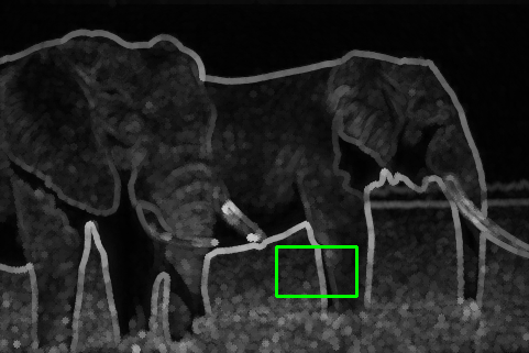
(d)

(e)

(f)

(g)

(h)

(i)

(j)

(k)

(l)

Figure 2: Dilation and erosion transformation where the structuring element is disk (3) applied to a sample image from the BSD500 dataset Arbelaez et al. (2011).

These operations are increasing, hence: $f<g\Rightarrow\varepsilon_{b}(f)(x)<\varepsilon_{b}(f)(x)$ or$f<g\Rightarrow\delta_{b}(f)(x)<\delta_{b}(f)(x)$. In addition, the erosion is anti-extensive, while the dilation is extensive, hence:$f>=\varepsilon_{b}(f)(x)$ and $\delta_{b}(f)(x)>=f$.

By combining these two basic operations, we can build new ones, such as the opening and closing. The opening of image $f$ by structuring element $b$ is given by applying an erosion on $f$ with the structuring element $b$ and then applying a dilation to the previous results with the same SE. The closing operation is the morphological dual to the opening.

$$\gamma_{b}(f)=\delta_{b}\left(\varepsilon_{b}(f)\right)\mbox{ , and }\varphi_{b}(f)=\varepsilon_{b}\left(\delta_{b}(f)\right).$$ (2)

By combining these two basic operations, we can also build the internal gradient and the external gradient, denoted respectively as $G_{i}$ and $G_{e}$ and defined as: $G_{e}(f)=\delta_{b}(f)-f\mbox{ , and }G_{i}(f)=f-\varepsilon_{b}(f)$.

In addition, we can also build the morphological gradient, which is the difference between the dilation and the erosion with the same SE applied to the same image. Hence, it is defined as: $G_{b}(f)=\delta_{b}(f)-\varepsilon_{b}(f)$. The structuring element impacts the morphological operations through both the geometry of its support and its weights. Hence, by combining the morphological operators, we can build new operators. The question arises as to how to combine these operators to achieve the best performance for a given task. These operators have long been combined based on expert knowledge, but in this work, we propose combining them using an architecture search algorithm.

3.2 Our Pseudo Morphological Dilation

We propose the pseudo morphological dilation operation, which is composed of the following steps:

1. We apply a traditional convolution operation to transform the feature map from $(C,H,W)$ into $(C\times r\times r,H,W)$, where $r$ represents the size of the convolution kernel, and $H$ and $W$ respectively represent the height and width of the image. Hence, we increase the number of feature map channels. Each feature map represents a neighborhood map that will be used in the step. For example, in Figure 3(a), we have four feature maps. We denote this step the projection convolution step. Let us denote $f$ as the input image and $\omega$ as the convolution kernel of spatial size $1\times 1$, and $b$ as the bias of the projection convolution. Let us consider that the convolutional layer has $C_{\mbox{in}}$ input channels and $C_{\mbox{out}}$ output channels. Hence, the resulting feature map at pixel $n_{1},n_{2}$ is equal to:

   $$g[n_{1},n_{2},c]=\sum_{k=0}^{C_{\mbox{in}}}f[n_{1},n_{2},k]\omega[0,0,k]+b[c]\mbox{ , with }k_{2}\in[1,C_{\mbox{out}}]$$ (3)

2. We then apply the pixel shuffle transformation to the feature maps representing the coordinates, as illustrated in Figure 3(b). The pixel shuffle transformation, also known as the sub-pixel convolution, was introduced in Shi et al. (2016) for the super-resolution task. The pixel shuffle transformation reorganizes the low-resolution image channels to obtain a bigger image with fewer channels. Specifically, it increases the spatial size of the feature map by reducing the number of channels. Hence, it rearranges the input tensor elements, expressed as $(C\times r\times r,H,W)$, to form a scaled $(C,H\times r,W\times r)$. This operation is interesting since it is stable, compatible with deep learning back propagation, and does not add artifacts. We denote this step the pixel shuffle step. More formally, each channel $c$ of the previous step represents a neighborhood, as illustrated in Figure 3. Let us decompose equation 3 into two terms such that for all $c$ we have $g[n_{1},n_{2},c]=\tilde{f}[n_{1},n_{2},c]+b[c]$, where $\tilde{f}$ is the results of the cross correlation of the convolution layer. Note that $C_{\mbox{out}}=r^{2}C_{\mbox{in}}$. The output of the pixel shuffle is:

   $$h[n_{1},n_{2},c]=g[\lfloor n_{1}/r\rfloor,\lfloor n_{2}/r\rfloor,c^{\prime}]$$ (4)

   where $\lfloor n_{1}/r\rfloor$ is the floor fraction, which takes as input a real number $n_{1}/r$ and outputs the greatest integer value. The channel $c^{\prime}$ is equal to $c^{\prime}=c+n_{1}\mbox{.mod}(r)+n_{2}\mbox{.mod}(r)+r\mathbf{1}_{n_{2}\mbox{.mod}(r)>0}$, where :$n_{1}{\mbox{.mod}(r)}=n_{1}-(\lfloor n_{1}/r\rfloor\times r)$.

3. On the output of the pixel shuffle step, we apply a max-pooling of stride $r$. We denote this step the max-pooling step. We apply the max-pooling into $h$ with a kernel of spatial size $r\times r$ and a stride $r$; let us denote $h^{\prime}$ as the result. Then, $h^{\prime}$ is equal to:

   $$h^{\prime}[n_{1},n_{2},c]=\max_{(i,j)\in\mathcal{N}}\tilde{f}[\lfloor(n_{1}+i)/r\rfloor,\lfloor(n_{2}+j)/r\rfloor,c^{\prime}[i,j]]+b[c^{\prime}[i,j]]$$ (5)

   where $c^{\prime}[i,j]=c+(n_{1}+i)\mbox{.mod}(r)+(n_{2}+j)\mbox{.mod}(r)+r\mathbf{1}_{(n_{2}+j)\mbox{.mod}(r)>0}$. Thus, we obtain a dilation on $\tilde{f}$, where the bias $b$ is the structuring element, with the connectivity depending on the channel.

Classical morphological operators can be hard to train due to the non-linearity, as pointed out in Franchi et al. (2020), where the authors proposed clipping the gradients of these layers and applying specific learning to them. Hence, integrating them into a NAS framework can be challenging as the NAS framework will try to learn the best architecture with the set of operations. Thus, we cannot build a hand-designed architecture that will stabilize the new layers, and the new layers must be stable for any architecture. Therefore, we propose a stable version, as introduced in this section.

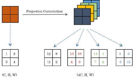
(a)

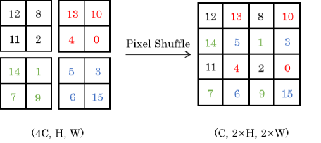
(b)

Figure 3: A simple example to explain the projection convolution and pixel shuffle step. We start with a feature map composed of 4 pixels of value (1,2,3,4) and then apply the projection convolution, with four feature maps of values (12,8,11,2),(13,10,4,0),(14,1,7,9) and (5,3,6,15). Then, by applying the pixel shuffle, we obtain just one feature map.

The full layer is represented in Figure 4. We simulate the structuring element’s shape by working with the parameter $r$ of the max-pooling and the pixel shuffle layer. We notice that by adding batch normalisation Ioffe and Szegedy (2015) before the projection convolution step, the results become more stable. Hence, we use it on all our layers. We denote this layer as a pseudo dilation because it is neither an increasing function nor an extensive function between the input and the output. Nonetheless, it checks these properties between the input and output of the max-pooling.

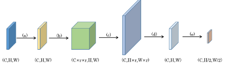
Figure 4: An overview of pseudo morphological dilation, pool, and erosion. The transformation is composed of 4 mandatory steps (a),(b),(c),(d) and one optional step (e). (a) Batch normalisation to transform the input feature maps. (b) Traditional convolution to transform the feature map from (C, H W) into (C×r×r, H, W). (c) A sub-pixel convolution that makes the length and weight of the feature map expand by r times. (d) Max-pooling or min-poling if we perform a dilation or an erosion, respectively, that makes the output feature map dimension consistent with the input feature map. (e) An optional max-pooling operation with a stride of 2.

3.3 Our Morphological Layers

Based on the description of our pseudo morphological dilation, which is our base operator, we describe four more operators in this sub-section: pseudo morphological erosion, pseudo morphological pooling, pseudo morphological upsampling, and pseudo morphological gradient.

The pseudo morphological erosion is constructed with the same exam step as the pseudo morphological dilation, except that instead of doing a max-pooling after the pixel shuffle step, we apply a min-pooling. We propose this operation to check the usefulness of such an operation based on the minimum. We illustrate this layer in Figure 4.

Similar to convolution layers with stride, we propose pseudo morphological pooling. This operation consists of first applying a pseudo morphological dilation operation, followed by an extra max-pooling, as shown in Figure 4. In other words, by using this approach we achieve the downsampling of the input image.

We propose pseudo morphological upsampling, which is similar to a deconvolution layer, for edge detection and semantic segmentation tasks. This operation is implemented by transforming the feature map from $(C,H,W)$ into $(r^{2}\times s^{2}\times C,H,W)$ through the projection convolution step. Then, we apply the pixel shuffle step to form feature maps with the size $(C,r\times s\times H,r\times s\times W)$. Subsequently, we apply the max-pooling step with stride $r$.

We propose a new layer called the pseudo morphological gradient. For this layer, we achieve the same projection convolution step, and pixel shuffle step. Then, we obtain pseudo morphological dilation feature maps using max-pooling, and we obtain the final gradient feature map by performing vector subtraction with the input image. Contrary to the morphological gradient, which is positive for all pixels, this one is not necessarily positive. This also happens with the morphological Laplacian Serra (1988), which is of interest for the denoising of images. Also, the skip connection provided by this gradient layer can help to avoid vanishing gradients. This layer is illustrated in Figure 5.

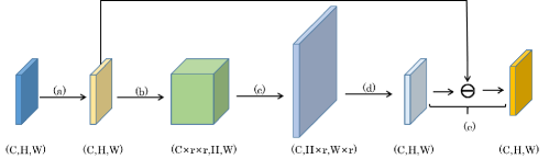
Figure 5: Overview of the pseudo morphological gradient. The process of (a)(b)(c)(d) is the same as with pseudo morphological dilation. (e) The vector subtraction used to obtain the external pseudo gradient.

3.4 Neural Architecture Search (NAS)

NAS recently identified DNN architectures that exceed human-designed ones in image classification Liu et al. (2019a); Luo et al. (2019). As illustrated in Figure 6, NAS needs three key elements:

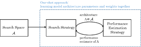
Figure 6: Components of the Neural Architecture Search (NAS) model

1. Search Space: This defines the set of operations (e.g. convolution, fully-connected, pooling) and how we want them to be connected to build valid network architectures. In a sense, the search space defines the space for the admissible solution.

2. Search algorithm: This is the algorithm used to optimize the architecture

3. Criterion: This defines the measure used to estimate or predict the performance of an architecture.

The criterion used for all the different tasks is the accuracy criterion applied to the validation; we want to optimize this for the given task. The remainder of this section describes our search space and search algorithm.

3.4.1 Search Space - Cell Search

In the NAS community, the search space represents the space in which we search the DNN’s architecture. The search space is composed of a set of operations and a backbone explaining how operations can be connected to construct valid network architectures. The search space can be classified into two categories. The first one is the Global Search Space, where the algorithm has to learn all the DNN architecture. The second one is the Cell-Based Search Space, where the DNN architecture lies in a backbone composed of basic components called cells, and the goal is to learn what is inside the cells. Inspired by DNN architecture such as ResNet He et al. (2016) or VGG Simonyan and Zisserman (2014b) , the author of NASNET Zoph et al. (2018), who initially proposed Cell-Based Search Space, noted that DNNs are composed of blocks with the same kind of operations that are repeated multiple times. Figure 7 presents the backbone of a DNN model for CIFAR10 Krizhevsky (2009).

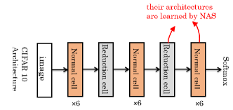
Figure 7: The overall backbone of a cell-based DNN model for CIFAR 10.

The Cell-Based Search Space appears to be a more popular alternative than the Global Search Space because the newly discovered neural architecture based on it can be easily transferred between datasets. Two sorts of cells are commonly employed for classification. The first is the standard cell, which preserves the feature map’s spatial size, and the second is the reduction cell, which shrinks the feature map’s spatial size.

Cell search space for classification

We tested three cell search spaces for the classification task: two with the morphological layer and one without. The different search spaces are illustrated in Table 1.

Cell search space	Cell search space	Cell search space
without morphological layer	with dilation	with erosion
	separable conv $3\times 3$
	separable conv $5\times 5$
	average pooling
	maximum pooling
$\oslash$	pseudo morphological dilation $3\times 3$	pseudo morphological erosion $3\times 3$

Table 1: Cell search space for the classification task. Separable conv $3\times 3$ and separable conv $5\times 5$ are the separable convolutions introduced in Chollet (2017), with kernel sizes of $3\times 3$ and $5\times 5$.

Cell search space for edge detection and semantic segmentation

For the edge detection and semantic segmentation tasks, we respectively propose three cell search spaces and one cell search spaces composed of six operations. To study the influence of pseudo morphological operations, all the search spaces have the same number of operations. The different search spaces are illustrated in Table 2.

Cell search space	Cell search space	Cell search space
without morphological layer	with dilation	with erosion
	cweight $3\times 3$
	separable conv $3\times 3$
	conv $3\times 3$
	average pooling
	maximum pooling
separable conv $5\times 5$	pseudo morphological dilation $3\times 3$	pseudo morphological gradient $3\times 3$

Table 2: Cell search space for the edge detection and semantic segmentation tasks. cweight $3\times 3$ is the Squeeze-and-Excitation Network (SENet) introduced in Luo et al. (2019), with a kernel size of $3\times 3$.

3.4.2 Search Space of the Architecture

As illustrated in Figure 7, the search architecture space is a backbone designed by repeating multiple modules composed of reduction cells and normal cells for classification. For the classification task, we do not change the search architecture space. However, we propose a search architecture space for the segmentation tasks, where the DNNs play with multiple resolutions, skip connections, and deconvolution.

U-Net architecture search space The U-Net architecture Ronneberger et al. (2015) inspired our first search architecture space, which we denote U-Net search space. We start with this search space since U-Net is the state-of-the-art for medical images.

The U-Net architecture is a fully convolutional network that reinjects the decoder feature map from the encoder information. Hence, the spatial information might be more precise.

Our U-Net search space backbone is similar to the U-Net DNN backbone. However, it is composed of two types of cell: a downsampling segmentation cell and an upsampling segmentation cell, which we denote DownSC and UpSC, respectively. The upsampling segmentation cell is composed of the following operations:

• separable conv $3\times 3$

• separable conv $5\times 5$

• average pooling

• maximum pooling

• pseudo mophological gradient $3\times 3$

• transpose convolution

The overall U-Net search backbone is presented in Figure 8.

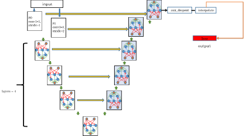
Figure 8: The overall backbone of the Cell-Based U-net Ronneberger et al. (2015)Weng et al. (2019), where C equals 8, B represents the number of intermediate nodes, H0 equals 0.25H, H1 equals 0.5H0, and the rest can be done in the same manner. The value of W is derived in the same way. In addition, the aux_dropout is an operation sequential.

Multi-scale decoder architecture search space

Inspired by Deeplab V3+ Chen et al. (2018), PSPNet Zhao et al. (2017), and RCFLiu et al. (2019b), we notice that a good architecture for general images relies on an encoder pretrained on ImageNetRussakovsky et al. (2015) and a decoder that takes multiple resolutions as input and associates them to build the output. Based on that, we propose our new network search space, which we denote the multi-scale decoder search network space.

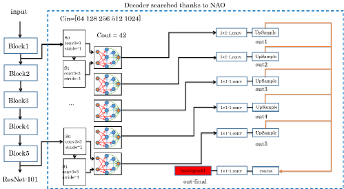
Figure 9: ResNet101_Decoder

First, we introduce RCF Liu et al. (2019b). The RCF algorithm proposes using a classical backbone such as the VGG16 Simonyan and Zisserman (2014a) architecture, composed of 13 convolutional layers and three fully connected layers. The 13 convolutional layers can be subdivided into five blocks. On each block, three convolutions are applied, leading to a feature map for each block. These different feature maps extract information at different resolutions, leading to a multi-scale representation. This hierarchical information is then merged to form the final output.

Our new network search space, illustrated in Figure 9, can be summarized as follows. We use a ResNet architecture He et al. (2016) pretrained on ImageNetRussakovsky et al. (2015) as an encoder network, similar to Chen et al. (2018); Zhao et al. (2017); Liu et al. (2019b). ResNet is composed of 4 blocs. We connect each block’s output to two layers. The first one is a preprocessing layer that we denote $S_{0}$. This layer is composed of a $3\times 3$ convolution and outputs 42 feature maps. This operation allows us to control the depth map that will enter the cells. The second preprocessing layer, applied on the output of $S_{0}$ and denoted $S_{1}$, is composed of a $3\times 3$ convolution and outputs 42 feature maps. The inputs of the cells are the outputs of $S_{0}$ and $S_{1}$, so that the cell learns if it wants to use $S_{0}$ and/or $S_{1}$. After each block, we use a $1\times 1$ convolution on the cells’ output to reduce the channel’s number to one. This convolution is followed by an upsampling to resize all the feature maps to input size, and we concatenate all the upsampled results. Finally, we use a $1\times 1$ to produce the final edge detection map.

DeeplabV3+ architecture search space

Similarly to Deeplab v3+ Chen et al. (2018), our new network search space, illustrated in Figure 10, can be summarized as follows. It is based on an Atrous Spatial Pyramid Pooling (ASPP), which is able to encode multi-scale contextual information. After having concatenated the output of the ASPP with a low-level feature like Deeplab v3+, we replace the $3\times 3$ convolution by a cell wherein we search for the operations.

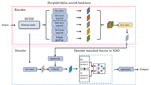
Figure 10: DeeplabV3+ architecture search space

3.4.3 Neural Architecture Optimization (NAO)

NAO Luo et al. (2019) is an optimization algorithm that searches for the best architectures based on the following principle. First, NAO is a Cell-Based Search Space algorithm, like most modern NAS. Hence, we merely need to learn the adjacency matrix that represents the cells. Secondly, NAO is a two-step algorithm that first searches for the best architecture in step 1. Then, in step 2, with this architecture, NAO optimizes the DNN’s weights to search for the best model. Thirdly, NAO does not directly optimize the cell parameters, and it performs its optimization on a latent space of cell parameters.

The NAO process is illustrated in Figure 11. In detail, the NAO algorithm consists of an encoder, a predictor, and a decoder networkLuo et al. (2019). The encoder of NAO Luo et al. (2019) takes as input a randomly generated architecture sequence describing an architecture, and then maps it onto a continuous space C. Specifically, the encoder is denoted as $\mathrm{E}:\mathrm{X}\rightarrow\mathrm{C}$. Let us write $e_{x}=E(x)$ as the latent representation of the DNN architecture.

The performance predictor Luo et al. (2019) $\mathrm{P}:\mathrm{C}\rightarrow\mathrm{R}$ maps the latent representation of an architecture x onto its performance $s_{x}$. With an architecture $x$ and its performance $s_{x}$ as training data, the optimization of $P$ aims to minimize the least-square regression $\text{loss }=\left(s_{x}-P(E(x))\right)^{2}$.

The decoder of NAO Luo et al. (2019), which is similar to the decoder in the DNN model, is responsible for decoding out the string tokens in $x$, taking $e_{x}$ as input. Mathematically, the decoder is denoted as function $\mathrm{D}:\mathrm{C}\rightarrow\mathrm{X}$, which decodes the input taking $e_{x}$. The training process consists of optimizing the following loss: $\sum_{x\in X}\log P_{D}(x\mid E(x))$.

The encodee-decoder learns to build a latent space that can represent the space of the architecture. The performance predictor learns to map this space onto its performance for the given task. Finally, a new architecture is generated by trying to determine which one has the best performance.

In this work, NAO was our preferred NAS method for the following three reasons:

• NAO incorporates recent search strategies to reduce the computational cost (a Cell-Based Search Space and weight sharing).

• NAO can be executed with a small computational time.

• NAO allows the easy customization of the backbone architecture.

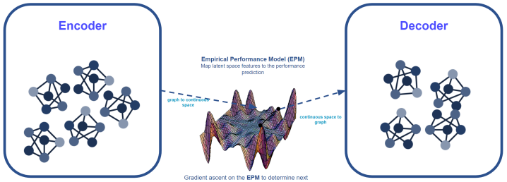
Figure 11: Overview of the NAO algorithm. The encoder maps architecture $x$ onto a continuous space represented by $e_{x}$. Afterwards, the predictor optimizes $e_{x}$ by maximizing the output of performance using gradient descent. The output of the predictor is represented as $e_{x^{\prime}}$. The decoder transforms $e_{x^{\prime}}$ into a new discrete architecture $x^{\prime}$Luo et al. (2019)

4 Experiments

In this section, we explain the experiments confirming our morphological layers’ utility. We consider three different types of experiments: classification, edge detection and semantic segmentation.

4.1 Classification task

We evaluate our layers on two datasets, CIFAR10Krizhevsky (2009) and CIFAR100Krizhevsky (2009), which are composed of 50 000 RGB training images and 10 000 RGB test images of the size $32\times 32$. CIFAR10 has 10 classes, while CIFAR100 has 100 classes. To train the DNN, we used the cross-entropy loss and reported the classification error, and we used the same experimental protocol as NAO uses for CIFAR 10. During the architecture search, we use a small network with $B=5$ (number of nodes), $N=3$ (number of normal cells), and $F=8$ (number of channels), and search the architecture for four iterations; each of them is composed of 50 epochs. After the best cell architectures are found, we increase the architecture with $B=5$, $N=6$, $F=36$ and optimize the weight of the DNNs for 600 epochs. The batch size for the two-step is 128. The results in Table 3 are the mean of 3 seeds. The mean error of our architecture with the morphological layer is 2.65%, which is below the 2.93% of NAO Luo et al. (2019). After attempting to replace the morphological dilation with erosion, we see that the result decreases. Hence, we noted on CIFAR 10 that the morphological dilation layer improves the performance of the DNN. We also note from Figure 12 that NAO uses this operation since it is present in 3 out of the 15 edges for the normal cell and 4 out of the 15 edges for the reduction cell. Morphological operations seem to bring information not presented by traditional convolutional layers, which can help to improve performance. Moreover, it seems that the training with the BN has a positive effect since it enables the performance to improve from 2.84 to 2.65

Figure 12 illustrates the normal and reduction cell structures that we learned for the CIFAR10 Krizhevsky (2009) classification task. The cells are represented by a graph, which can be characterized by an adjacency matrix as drawn in Figure 12.

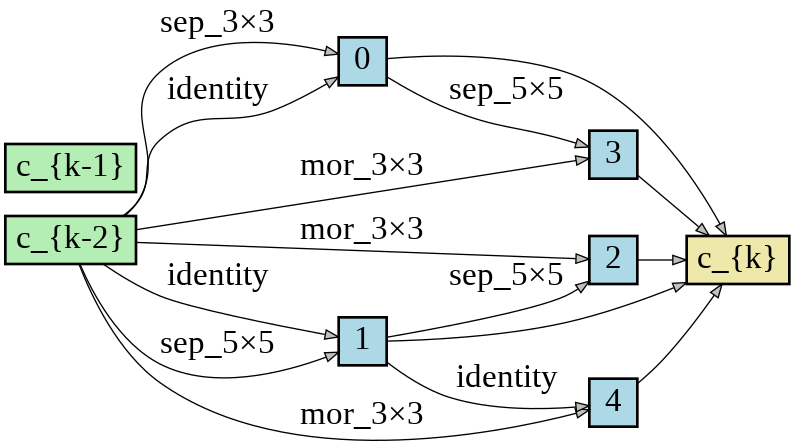
(a)

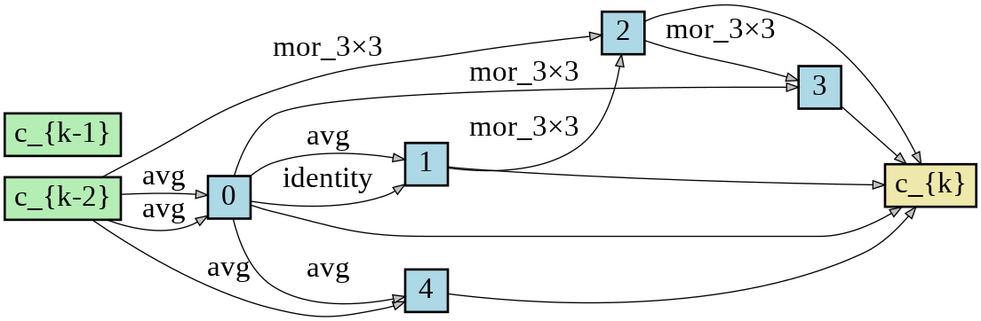
(b)

(c)

Figure 12: (a) and (b) represent the cell structure for the classification of CIFAR10, where $c_{k-1}$ represents the previous output and $c_{k-2}$ represents the output of the cell just before $c_{k-1}$. The blue numbers 0-4 represent the intermediate nodes, and every edge represents different operations. In addition, $c_{k}$ represents the output of the current cell, which concatenates the results of the intermediate node 0-4. (c) represents the adjacency matrix for the normal cell and the reduction cell. From left to right: the adjacency matrix of the normal cell, the adjacency matrix of the reduction cell. Among them, the numbers 1,2,3,4,5,6, and 7 respectively represent the following layers: separable conv $3\times 3$, separable conv $5\times 5$, avg pool, max pool, identity, pseudo morphological dilation $3\times 3$, and concatenate operation.

We also train an architecture search on CIFAR100 and check that we can confirm our previous result. Table 4 presents our results for CIFAR100. We note that the morphological layer seems to improve the performance of the classification task. Furthermore, training from scratch on the architecture search on CIFAR100 brings worse results than transferring the architecture learned on CIFAR10.

Method	B	Error(%)	GPU Days
ResNet with stochastic depthHuang et al. (2016)		5.25	0.63
Wide ResNetZagoruyko and Komodakis (2017)		4.00	/
ENAS+CutoutPham et al. (2018)	$5$	3.54	0.45
Block-QNN-S more filtersZhong et al. (2018)		3.54	3
DenseNet-BCHuang et al. (2018)		3.46	/
PNAS+CutoutLiu et al. (2018)	$5$	3.41	225
DARTS+CutoutLiu et al. (2019a)	$5$	$2.83$	4
MergeNAS(2nd-order)+cutoutWang et al. (2020)		$2.68$	0.6
PC-DARTS+cutoutXu et al. (2019)		$2.57$	0.1
few-shot DARTS-Small+cutoutZhao et al. (2020)		$2.31$	1.35
One-Stage ISTAYang et al. (2020)		$2.36$	2.3
NAONet-WSLuo et al. (2019)	$5$	$3.53$	0.3
NAONet-WS+CutoutLuo et al. (2019)	$5$	$2.93$	0.3
NAONet-WS+Cutout+
pseudo morphological dilation without BN	$5$	2.84	0.3
NAONet-WS+Cutout+
pseudo morphological dilation	$5$	2.65	0.3
NAONet-WS+Cutout+
pseudo morphological erosion	$5$	$3.20$	0.3

Table 3: CIFAR10 Performance of NAONet with pseudo morphological operations, where B represents the number of nodes within the cell. Error represents the accuracy error.

Method	B	Error(%)
ResNet with stochastic depthHuang et al. (2016)		24.98
Wide ResNetZagoruyko and Komodakis (2017)		19.25
Block-QNN-S more filtersZhong et al. (2018)		18.06
PNAS+Cutout∗Liu et al. (2018)	$5$	$17.44$
DenseNet-BCHuang et al. (2018)		17.18
ENAS+Cutout∗Pham et al. (2018)	$5$	$16.44$
One-Stage ISTAYang et al. (2020)		$16.9$
DHAZhou et al. (2021)		$16.07$
NAONet-WS+Cutout∗Luo et al. (2019)	$5$	15.67
NAONet-WS+Cutout+
without pseudo morphological dilation	$5$	16.9
NAONet-WS+Cutout+
pseudo morphological dilation	$5$	16.23

Table 4: CIFAR100 Performance of NAONet with pseudo morphological operations, where B represents the number of nodes within the cell. Error represents the accuracy error. Please note that the results of the techniques with a star ^∗ train the architecture search on CIFAR10 and learn the model on CIFAR 100.

4.2 Edge detection task

We propose a method for extracting image edges to highlight the power of morphological operators in deep learning frameworks. We recommended two backbones for this task: the U-Net search backbone and the multi-scale decoder architecture search space. These are detailed in section 3.4.2.

We train our DNNs on BSDS500 Arbelaez et al. (2011), which comprises 200 training, 100 validation, and 200 test images. Up to 9 annotators labeled each image. Like previous works Liu et al. (2019b); Liu and Lew (2016); Yang et al. (2016); Kokkinos (2015), we use the training set and validation set for tuning the DNN and the test set for the evaluation and mix the augmented training data of BSDS500 with the flippedVOC Context dataset Mottaghi et al. (2014).

On medical images, the U-Net backbone offers state-of-the-art performance for semantic segmentation, yet as illustrated in Table 5, this backbone does not give good results for edge detection. Subsequently, we propose a multi-scale decoder architecture search space that we denote NAO-Multi-scale. This backbone is inspired by traditional algorithms Wen et al. (2018) that perform well on this task. This algorithm learns a decoder using an encoder pre-trained on ImageNet Russakovsky et al. (2015).

To evaluate our novel algorithm, we use the F1-score, which is the harmonic average of the precision and recall and ranges between 0 and 1, with higher values being better. We evaluate the F1 score for each image of the test set of BSDS500 Arbelaez et al. (2011) at different thresholds for the edge prediction. We apply different thresholds since our results are edge probabilities with values between zero and one. The closer to one the edge value is, the more likely this edge is to be correct. However, this metric does not provide a result for the entire dataset. Hence, similar to Liu et al. (2019b); Liu and Lew (2016); Yang et al. (2016); Kokkinos (2015), the Optimal Dataset Scale (ODS) and Optimal Image Scale (OIS) are used to provide a metric for the whole dataset.

The Optimal Dataset Scale (ODS), where one chooses the optimal threshold for the entire dataset before applying the F1 score, and the Optimal Image Scale (OIS), where one chooses the optimal threshold per-image before using the F1 score, are two metrics for evaluating the quality of the edge detection algorithm on the whole dataset. The OIS is always slightly better than the ODS since it considers the best scale for each image. The OIS corresponds to the optimistic situation where we have the optimal threshold for each image of the dataset. For more information about these classical measures for edge detection, refer to Arbelaez et al. (2011)Liu et al. (2019).

Figure 13 presents examples of where RCF is unable to detect edges, while Figure 14 offers examples of where RCF detects edges where there are no edges. Finally, Figure 15 gives some examples of where our algorithm fails.

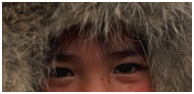
(a)

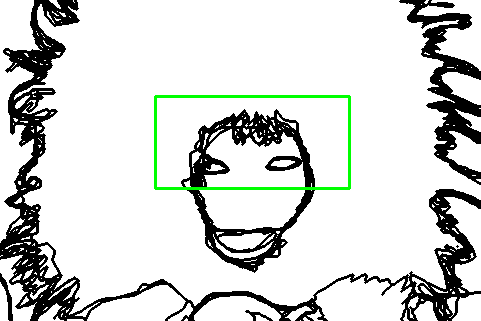
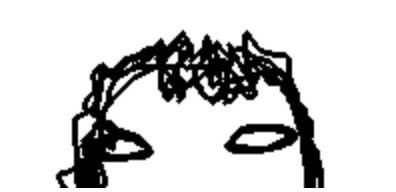
(b)

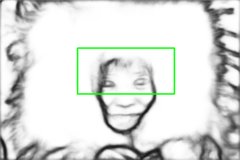
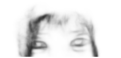
(c)

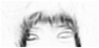
(d)

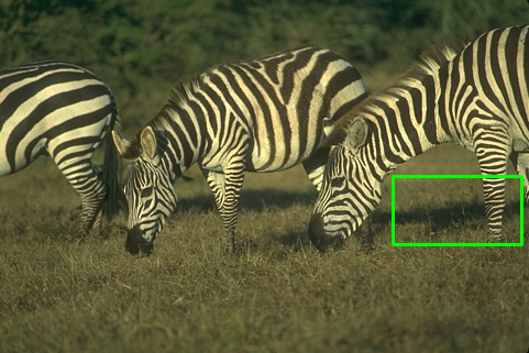
(e)

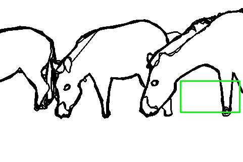
(f)

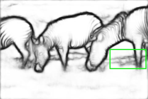
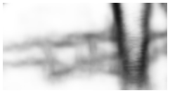
(g)

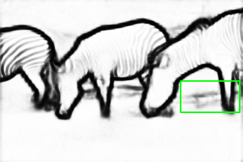
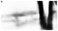
(h)

Figure 13: Overview of the results of different methods on BSD500 Arbelaez et al. (2011). From left to right: original image, ground truth, RCF Liu et al. (2019b) predicted edge map, and NAO_multi_scale predicted edge map. We can see in these examples that RCF has more false negatives than NAO_multi_scale.

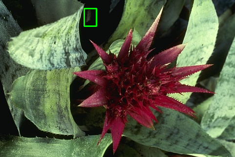
(a)

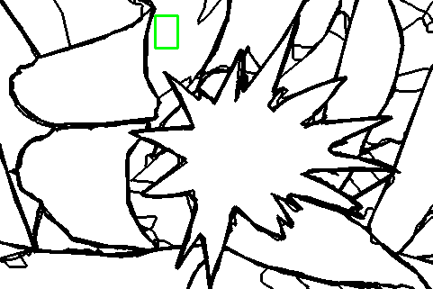
(b)

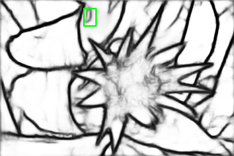
(c)

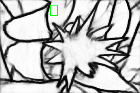
(d)

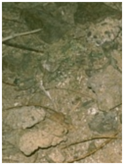
(e)

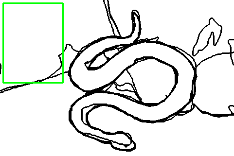
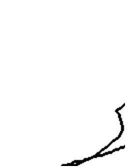
(f)

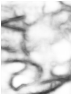
(g)

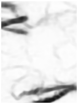
(h)

Figure 14: Overview of the results of different methods on BSD500 Arbelaez et al. (2011). From left to right: original image, ground truth, RCF Liu et al. (2019b) predicted edge map, and NAO_multi_scale predicted edge map. We can see in these examples that RCF has more false positives than NAO_multi_scale.

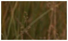
(a)

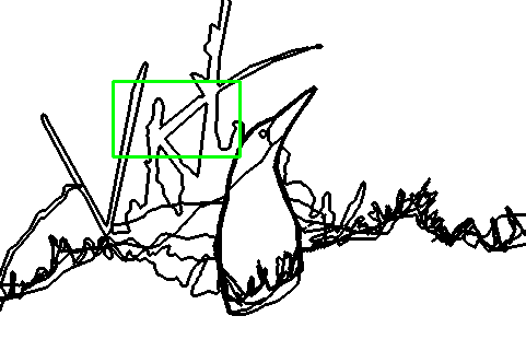
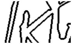
(b)

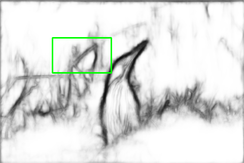
(c)

(d)

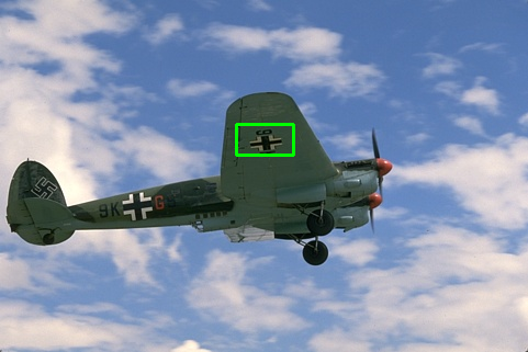
(e)

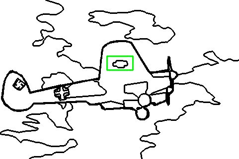
(f)

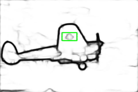
(g)

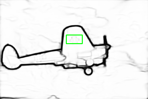
(h)

Figure 15: Overview of the results of different methods on BSD500 Arbelaez et al. (2011). From left to right: original image, ground truth, RCFLiu et al. (2019b) predicted edge map, and NAO_multi_scale predicted edge map. We can see in these examples that NAO_multi_scale has more false negatives than RCF.

Method	ODS	OIS	AP	R50
DeepEdge Bertasius et al. (2015a)	0.753	0.772	0.807
$N^{4}$-Fields Ganin and Lempitsky (2014)	0.753	0.767	0.780
HFL Bertasius et al. (2015b)	0.767	0.788	0.800
HED Xie and Tu (2015a)	0.782	0.804	0.833
RDS Liu and Lew (2016)	0.792	0.810
CEDN Yang et al. (2016)	0.788	0.804
AMH-Net(fusion) Xu et al. (2018)	0.798	0.829	0.869
CED Wang et al. (2019)	0.803	0.820	0.871
MIL+G-DSN+VOC+MS+NCuts Kokkinos (2015)	0.813	0.831
RCF_ResNet101 Liu et al. (2019b)	0.812	0.829
RCN-VOC-1Kelm et al. (2019)	0.812	0.827	0.822
CATS-BDCNHuan et al. (2021)	0.812	0.828
NAO-U-NET(ours)	0.788	0.808	0.814	0.899
with dilation search space
NAO-Multi-scale(ours) without morphological search space	0.812 $\pm 0.001$	0.830 $\pm 0.001$	0.827$\pm 0.014$	0.903$\pm 0.00471$
NAO-Multi-scale(ours) with dilation search space	0.809 $\pm 0.001$	0.829 $\pm 0.001$	0.825 $\pm 0.0149$	0.900 $\pm 0.0048$
NAO-Multi-scale(ours) with gradient search space	0.814 $\pm 0.001$	0.831 $\pm 0.001$	0.850$\pm 0.002$	0.908 $\pm 0.005$

Table 5: Performance of NAO_ResNet in comparison with other competitors on the BSD500 test set, measured using the method of Xie and Tu (2015b). For our experiments, the results are presented as mean $\pm std-dev$ computed from 3 runs.

In Table 5, our results for NAO-Multi-scale outperform the state-of-the-art results when we use the gradient search space. This is because the gradient can be used to detect edges; hence, using this layer helps the DNN to estimate the edge detection.

4.3 Semantic Segmentation Task

We propose adapting Deeplab v3+ Chen et al. (2018) and learning one deconvolution cell. The Deeplab v3+ backbone is detailed in section 3.4.2. We train our DNNs on Cityscape Cordts et al. (2016), which comprises 2975 training and 500 validation images. Our results in the validation split are given in Table 6. We note that the morphological operations help to improve the mIoU on the validation, leading to more accurate DNNs. Moreover, our Deeplab v3+ backbone improves the performance of the classical Deeplab v3+.

		MIou(Cityscapes)
Deeplabv3plus Chen et al. (2018)	Official result	76.9
NAO-Deeplabv3plus with morpho	arc_300_100 batch size=12	77.23
NAO-Deeplabv3plus without morpho	arc_300_100 batch size=12	76.97

Table 6: Performance of NAO-Deeplab v3+ in comparison with the official Deeplab v3+ on the Cityscape Cordts et al. (2016) validation set.

4.4 Discussion

We demonstrated in prior experiments that morphological layers boost the DNN’s performance for a specific architecture search methodology. However, the improvement is not consistent across all levels. As seen in Table 3, erosion layers perform worse than DNN without morphological layers. However, dilation layers increase performance. This improvement is because erosion is associated with a min-pooling process that extracts less noticeable regions. Similarly, as seen in Table 5, the DNN learned with dilation layers degrades performance, whereas the gradient-based DNN improves it. This highlights how the correct choice of morphological layers can enhance the representational power of a DNN. Another intriguing element of the edge detection studies is that the search space of the architecture matters, as we observe that the U-Net search space produces worse results than the multi-scale decoder search space proposed here. As illustrated in Figures 13 and 14, multi-resolution aids in obtaining a better edge since some items may be more easily spotted at certain resolutions than others. Moreover, we note that the results obtained using the multi-scale decoder search space with the gradient layer are state-of-the-art, demonstrating the usefulness of these layers. Finally, we remark that our strategy of comparing the best architecture with and without morphological layers using NAS takes six days in total, irrespective of which search space we use. An alternative to NAS would be to design an experimental protocol to test all possible architecture configurations. However, such a search would be long and would depend on the exploration protocol. Hence, our protocol can be used to confirm the interest in using morphological layers.

5 Conclusion

This paper introduces a new layer for Deep Neural Networks that is based on mathematical morphology. We offer a novel equitable technique for determining the utility of a new layer and apply this method to our newly created layers. We conclude that our layer has the potential to be extremely useful for image categorization and edge detection. This evaluation methodology appears to be more equitable than the standard approach, which entails proposing a new layer and handcrafting an architecture to increase performance. In this case, everything is optimized using an algorithm.

Additionally, we suggest a new backbone architecture for the architecture search, wherein both the input and output are images; we refer to this as NAO-Multi-scale. Comparing it to the U-net architecture search, we establish that our search architecture shows superior performance. Finally, we achieve state-of-the-art edge detection performance using NAO-Multi-scale and gradient operations.

In future research, based on these encouraging results, we will examine how to employ such layers to conduct semantic segmentation. Additionally, it will be fascinating to deal with more specialized information, such as remote sensing data containing several photographs of buildings and roads with unique geometric shapes. As such, it may be instructive to observe how these new layers act in this scenario. We could also add transformer layers to the search, which was beyond the scope of this paper. We note that these layers show good results in computer vision tasks and aim to study them in future works.

Acknowledgments: This work was performed using HPC resources from GENCI-IDRIS (Grant 2020-AD011011970) and (Grant 2021-AD011011970R1).

References

- Krizhevsky et al. (2012) Alex Krizhevsky, Ilya Sutskever, and Geoffrey E. Hinton. Imagenet classification with deep convolutional neural networks. In International Conference on Neural Information Processing Systems, pages 1097–1105, 2012.
- Simonyan and Zisserman (2014a) Karen Simonyan and Andrew Zisserman. Very deep convolutional networks for large-scale image recognition. arXiv preprint arXiv:1409.1556, 2014a.
- He et al. (2016) Kaiming He, Xiangyu Zhang, Shaoqing Ren, and Jian Sun. Deep residual learning for image recognition. In Proceedings of the IEEE conference on computer vision and pattern recognition, pages 770–778, 2016.
- Redmon et al. (2016) Joseph Redmon, Santosh Divvala, Ross Girshick, and Ali Farhadi. You only look once: Unified, real-time object detection. In Proceedings of the IEEE conference on computer vision and pattern recognition, pages 779–788, 2016.
- Radford et al. (2019) Alec Radford, Jeffrey Wu, Rewon Child, David Luan, Dario Amodei, and Ilya Sutskever. Language models are unsupervised multitask learners. OpenAI Blog, 1:8, 2019.
- Liu et al. (2019a) Hanxiao Liu, Karen Simonyan, and Yiming Yang. Darts: Differentiable architecture search, 2019a.
- Luo et al. (2019) Renqian Luo, Fei Tian, Tao Qin, Enhong Chen, and Tie-Yan Liu. Neural architecture optimization, 2019.
- Liu et al. (2018) Chenxi Liu, Barret Zoph, Maxim Neumann, Jonathon Shlens, Wei Hua, Li-Jia Li, Li Fei-Fei, Alan Yuille, Jonathan Huang, and Kevin Murphy. Progressive neural architecture search. In Proceedings of the European conference on computer vision (ECCV), pages 19–34, 2018.
- Pham et al. (2018) Hieu Pham, Melody Guan, Barret Zoph, Quoc Le, and Jeff Dean. Efficient neural architecture search via parameters sharing. In International Conference on Machine Learning, pages 4095–4104. PMLR, 2018.
- Weng et al. (2019) Y. Weng, T. Zhou, Y. Li, and X. Qiu. Nas-unet: Neural architecture search for medical image segmentation. IEEE Access, 7:44247–44257, 2019. ISSN 2169-3536. doi:10.1109/ACCESS.2019.2908991.
- Rivest et al. (1993) Jean-Francois Rivest, Pierre Soille, and Serge Beucher. Morphological gradients. Journal of Electronic Imaging, 2(4):326–336, 1993.
- Serra (1988) Jean Serra. Image analysis and mathematical morphology, v. 2. Academic Press, 1988.
- Thibault et al. (2013) Guillaume Thibault, Jesus Angulo, and Fernand Meyer. Advanced statistical matrices for texture characterization: application to cell classification. IEEE Transactions on Biomedical Engineering, 61(3):630–637, 2013.
- Franchi and Angulo (2014) Gianni Franchi and Jesus Angulo. Comparative study on morphological principal component analysis of hyperspectral images. In 2014 6th Workshop on Hyperspectral Image and Signal Processing: Evolution in Remote Sensing (WHISPERS), pages 1–4. IEEE, 2014.
- Cavallaro et al. (2017) Gabriele Cavallaro, Nicola Falco, Mauro Dalla Mura, and Jón Atli Benediktsson. Automatic attribute profiles. IEEE Transactions on Image Processing, 26(4):1859–1872, 2017.
- Velasco-Forero and Angulo (2013) Santiago Velasco-Forero and Jesus Angulo. Classification of hyperspectral images by tensor modeling and additive morphological decomposition. Pattern Recognition, 46(2):566–577, 2013.
- Franchi and Angulo (2016) Gianni Franchi and Jesus Angulo. Morphological principal component analysis for hyperspectral image analysis. ISPRS International Journal of Geo-Information, 5(6):83, 2016.
- Franchi et al. (2020) Gianni Franchi, Amin Fehri, and Angela Yao. Deep morphological networks. Pattern Recognition, 102:107246, 2020. ISSN 0031-3203.
- Valle (2020) Marcos Eduardo Valle. Reduced dilation-erosion perceptron for binary classification. Mathematics, 8(4):512, Apr 2020. ISSN 2227-7390.
- Mondal et al. (2020) Ranjan Mondal, Moni Shankar Dey, and Bhabatosh Chanda. Image restoration by learning morphological opening-closing network. Mathematical Morphology-Theory and Applications, 4(1):87–107, 2020.
- Krizhevsky (2009) Alex Krizhevsky. Learning multiple layers of features from tiny images. Technical report, 2009.
- Martin et al. (2001) D. Martin, C. Fowlkes, D. Tal, and J. Malik. A database of human segmented natural images and its application to evaluating segmentation algorithms and measuring ecological statistics. In Proc. 8th Int’l Conf. Computer Vision, volume 2, pages 416–423, July 2001.
- Cordts et al. (2016) Marius Cordts, Mohamed Omran, Sebastian Ramos, Timo Rehfeld, Markus Enzweiler, Rodrigo Benenson, Uwe Franke, Stefan Roth, and Bernt Schiele. The cityscapes dataset for semantic urban scene understanding, 2016.
- Serra (1983) Jean Serra. Image Analysis and Mathematical Morphology. Academic Press, Inc., Orlando, FL, USA, 1983. ISBN 0126372403.
- Bouchet et al. (2016) Agustina Bouchet, Pedro Alonso, Juan Ignacio Pastore, Susana Montes, and Irene Díaz. Fuzzy mathematical morphology for color images defined by fuzzy preference relations. Pattern Recognition, 60:720–733, 2016.
- Franchi et al. (2018) Gianni Franchi, Jesus Angulo, Maxime Moreaud, and Loïc Sorbier. Enhanced edx images by fusion of multimodal sem images using pansharpening techniques. Journal of microscopy, 269(1):94–112, 2018.
- Cavallaro (2016) Gabriele Cavallaro. Spectral-Spatial Classification of Remote Sensing Optical Data with Morphological Attribute Profiles using Parallel and Scalable Methods. PhD thesis, University of Iceland, 2016.
- Dufour et al. (2013) Alice Dufour, Christian Ronse, Joseph Baruthio, Olena Tankyevych, Hugues Talbot, and Nicolas Passat. Morphology-based cerebrovascular atlas. In 2013 IEEE 10th International Symposium on Biomedical Imaging, pages 1210–1214. IEEE, 2013.
- Zhang et al. (2012) Xiwei Zhang, Guillaume Thibault, Etienne Decencière, Gwénolé Quellec, Guy Cazuguel, Ali Erginay, Pascale Massin, and Agnès Chabouis. Spatial normalization of eye fundus images. In ISBI 2012: 9th IEEE International Symposium on Biomedical Imaging. IEEE, 2012.
- Masci et al. (2013) Jonathan Masci, Jesús Angulo, and Jürgen Schmidhuber. A learning framework for morphological operators using counter–harmonic mean. In International Symposium on Mathematical Morphology and Its Applications to Signal and Image Processing, pages 329–340. Springer, 2013.
- Saeedan et al. (2018) Faraz Saeedan, Nicolas Weber, Michael Goesele, and Stefan Roth. Detail-preserving pooling in deep networks. In Proceedings of the IEEE Conference on Computer Vision and Pattern Recognition, pages 9108–9116, 2018.
- Mondal et al. (2019) Ranjan Mondal, Sanchayan Santra, and Bhabatosh Chanda. Dense morphological network: An universal function approximator. arXiv preprint arXiv:1901.00109, 2019.
- Charisopoulos and Maragos (2017) Vasileios Charisopoulos and Petros Maragos. Morphological perceptrons: geometry and training algorithms. In International Symposium on Mathematical Morphology and Its Applications to Signal and Image Processing, pages 3–15. Springer, 2017.
- Mellouli et al. (2017) Dorra Mellouli, Tarek M Hamdani, Mounir Ben Ayed, and Adel M Alimi. Morph-cnn: A morphological convolutional neural network for image classification. In International Conference on Neural Information Processing, pages 110–117. Springer, 2017.
- Nogueira et al. (2019) Keiller Nogueira, Jocelyn Chanussot, Mauro Dalla Mura, William Robson Schwartz, and Jefersson A. dos Santos. An introduction to deep morphological networks, 2019.
- Blusseau et al. (01 Jan. 2020) Samy Blusseau, Bastien Ponchon, Santiago Velasco-Forero, Jesús Angulo, and Isabelle Bloch. Approximating morphological operators with part-based representations learned by asymmetric auto-encoders. Mathematical Morphology - Theory and Applications, 4(1):64 – 86, 01 Jan. 2020.
- Zöller and Huber (2019) Marc-André Zöller and Marco F Huber. Survey on automated machine learning. arXiv preprint arXiv:1904.12054, 2019.
- Kitano (1990) Hiroaki Kitano. Designing neural networks using genetic algorithms with graph generation system. Complex systems, 4(4):461–476, 1990.
- Camero et al. (2020) Andrés Camero, Hao Wang, Enrique Alba, and Thomas Bäck. Bayesian neural architecture search using a training-free performance metric. arXiv preprint arXiv:2001.10726, 2020.
- Liu et al. (2021) Yuqiao Liu, Yanan Sun, Bing Xue, Mengjie Zhang, Gary G Yen, and Kay Chen Tan. A survey on evolutionary neural architecture search. IEEE Transactions on Neural Networks and Learning Systems, 2021.
- Loshchilov and Hutter (2016) Ilya Loshchilov and Frank Hutter. Cma-es for hyperparameter optimization of deep neural networks. arXiv preprint arXiv:1604.07269, 2016.
- Ren et al. (2020) Pengzhen Ren, Yun Xiao, Xiaojun Chang, Po-Yao Huang, Zhihui Li, Xiaojiang Chen, and Xin Wang. A comprehensive survey of neural architecture search: Challenges and solutions, 2020.
- Zoph et al. (2018) Barret Zoph, Vijay Vasudevan, Jonathon Shlens, and Quoc V Le. Learning transferable architectures for scalable image recognition. In Proceedings of the IEEE conference on computer vision and pattern recognition, pages 8697–8710, 2018.
- Song et al. (2021) Xingyou Song, Krzysztof Choromanski, Jack Parker-Holder, Yunhao Tang, Daiyi Peng, Deepali Jain, Wenbo Gao, Aldo Pacchiano, Tamás Sarlós, and Yuxiang Yang. ES-ENAS: combining evolution strategies with neural architecture search at no extra cost for reinforcement learning. CoRR, abs/2101.07415, 2021.
- Eiben and Smit (2011) Agoston E Eiben and Selmar K Smit. Parameter tuning for configuring and analyzing evolutionary algorithms. Swarm and Evolutionary Computation, 1(1):19–31, 2011.
- Angulo (2017) Jesus Angulo. Convolution in (max,min)-algebra and its role in mathematical morphology. In Advances in imaging and electron physics, volume 203, pages 1–66. Elsevier, 2017.
- Arbelaez et al. (2011) Pablo Arbelaez, Michael Maire, Charless Fowlkes, and Jitendra Malik. Contour detection and hierarchical image segmentation. IEEE Trans. Pattern Anal. Mach. Intell., 33(5):898–916, May 2011. ISSN 0162-8828.
- Shi et al. (2016) Wenzhe Shi, Jose Caballero, Ferenc Huszár, Johannes Totz, Andrew P. Aitken, Rob Bishop, Daniel Rueckert, and Zehan Wang. Real-time single image and video super-resolution using an efficient sub-pixel convolutional neural network, 2016.
- Ioffe and Szegedy (2015) Sergey Ioffe and Christian Szegedy. Batch normalization: Accelerating deep network training by reducing internal covariate shift. In International conference on machine learning, pages 448–456. PMLR, 2015.
- Simonyan and Zisserman (2014b) Karen Simonyan and Andrew Zisserman. Very deep convolutional networks for large-scale image recognition. arXiv preprint arXiv:1409.1556, 2014b.
- Chollet (2017) François Chollet. Xception: Deep learning with depthwise separable convolutions. In Proceedings of the IEEE conference on computer vision and pattern recognition, pages 1251–1258, 2017.
- Ronneberger et al. (2015) Olaf Ronneberger, Philipp Fischer, and Thomas Brox. U-net: Convolutional networks for biomedical image segmentation, 2015.
- Chen et al. (2018) Liang-Chieh Chen, Yukun Zhu, George Papandreou, Florian Schroff, and Hartwig Adam. Encoder-decoder with atrous separable convolution for semantic image segmentation. In Proceedings of the European conference on computer vision (ECCV), pages 801–818, 2018.
- Zhao et al. (2017) Hengshuang Zhao, Jianping Shi, Xiaojuan Qi, Xiaogang Wang, and Jiaya Jia. Pyramid scene parsing network. In Proceedings of the IEEE conference on computer vision and pattern recognition, pages 2881–2890, 2017.
- Liu et al. (2019b) Yun Liu, Ming-Ming Cheng, Xiaowei Hu, Jia-Wang Bian, Le Zhang, Xiang Bai, and Jinhui Tang. Richer convolutional features for edge detection. IEEE Transactions on Pattern Analysis and Machine Intelligence, 41(8):1939–1946, Aug 2019b. ISSN 1939-3539.
- Russakovsky et al. (2015) Olga Russakovsky, Jia Deng, Hao Su, Jonathan Krause, Sanjeev Satheesh, Sean Ma, Zhiheng Huang, Andrej Karpathy, Aditya Khosla, Michael Bernstein, Alexander C. Berg, and Li Fei-Fei. Imagenet large scale visual recognition challenge, 2015.
- Huang et al. (2016) Gao Huang, Yu Sun, Zhuang Liu, Daniel Sedra, and Kilian Weinberger. Deep networks with stochastic depth, 2016.
- Zagoruyko and Komodakis (2017) Sergey Zagoruyko and Nikos Komodakis. Wide residual networks, 2017.
- Zhong et al. (2018) Zhao Zhong, Junjie Yan, Wei Wu, Jing Shao, and Cheng-Lin Liu. Practical block-wise neural network architecture generation, 2018.
- Huang et al. (2018) Gao Huang, Zhuang Liu, Laurens van der Maaten, and Kilian Q. Weinberger. Densely connected convolutional networks, 2018.
- Wang et al. (2020) Xiaoxing Wang, Chao Xue, Junchi Yan, Xiaokang Yang, Yonggang Hu, and Kewei Sun. Mergenas: Merge operations into one for differentiable architecture search. In Christian Bessiere, editor, Proceedings of the Twenty-Ninth International Joint Conference on Artificial Intelligence, IJCAI-20, pages 3065–3072. International Joint Conferences on Artificial Intelligence Organization, 7 2020. doi:10.24963/ijcai.2020/424. Main track.
- Xu et al. (2019) Yuhui Xu, Lingxi Xie, Xiaopeng Zhang, Xin Chen, Guo-Jun Qi, Qi Tian, and Hongkai Xiong. Pc-darts: Partial channel connections for memory-efficient architecture search, 2019.
- Zhao et al. (2020) Yiyang Zhao, Linnan Wang, Yuandong Tian, Rodrigo Fonseca, and Tian Guo. Few-shot neural architecture search, 2020.
- Yang et al. (2020) Yibo Yang, Hongyang Li, Shan You, Fei Wang, Chen Qian, and Zhouchen Lin. Ista-nas: Efficient and consistent neural architecture search by sparse coding, 2020.
- Zhou et al. (2021) Kaichen Zhou, Lanqing Hong, Shoukang Hu, Fengwei Zhou, Binxin Ru, Jiashi Feng, and Zhenguo Li. Dha: End-to-end joint optimization of data augmentation policy, hyper-parameter and architecture, 2021.
- Liu and Lew (2016) Yu Liu and Michael S Lew. Learning relaxed deep supervision for better edge detection. In Proceedings of the IEEE conference on computer vision and pattern recognition, pages 231–240, 2016.
- Yang et al. (2016) Jimei Yang, Brian Price, Scott Cohen, Honglak Lee, and Ming-Hsuan Yang. Object contour detection with a fully convolutional encoder-decoder network. In Proceedings of the IEEE conference on computer vision and pattern recognition, pages 193–202, 2016.
- Kokkinos (2015) Iasonas Kokkinos. Pushing the boundaries of boundary detection using deep learning. arXiv preprint arXiv:1511.07386, 2015.
- Mottaghi et al. (2014) Roozbeh Mottaghi, Xianjie Chen, Xiaobai Liu, Nam-Gyu Cho, Seong-Whan Lee, Sanja Fidler, Raquel Urtasun, and Alan Yuille. The role of context for object detection and semantic segmentation in the wild. In Proceedings of the IEEE Conference on Computer Vision and Pattern Recognition, pages 891–898, 2014.
- Wen et al. (2018) Changbao Wen, Pengli Liu, Wenbo Ma, Zhirong Jian, Changheng Lv, Jitong Hong, and Xiaowen Shi. Edge detection with feature re-extraction deep convolutional neural network. Journal of Visual Communication and Image Representation, 57:84 – 90, 2018. ISSN 1047-3203.
- Liu et al. (2019) Y. Liu, M. Cheng, X. Hu, J. Bian, L. Zhang, X. Bai, and J. Tang. Richer convolutional features for edge detection. IEEE Transactions on Pattern Analysis and Machine Intelligence, 41(8):1939–1946, 2019. doi:10.1109/TPAMI.2018.2878849.
- Bertasius et al. (2015a) Gedas Bertasius, Jianbo Shi, and Lorenzo Torresani. Deepedge: A multi-scale bifurcated deep network for top-down contour detection. In Proceedings of the IEEE Conference on Computer Vision and Pattern Recognition, pages 4380–4389, 2015a.
- Ganin and Lempitsky (2014) Yaroslav Ganin and Victor Lempitsky. -fields: Neural network nearest neighbor fields for image transforms, 2014.
- Bertasius et al. (2015b) Gedas Bertasius, Jianbo Shi, and Lorenzo Torresani. High-for-low and low-for-high: Efficient boundary detection from deep object features and its applications to high-level vision, 2015b.
- Xie and Tu (2015a) Saining Xie and Zhuowen Tu. Holistically-nested edge detection, 2015a.
- Xu et al. (2018) Dan Xu, Wanli Ouyang, Xavier Alameda-Pineda, Elisa Ricci, Xiaogang Wang, and Nicu Sebe. Learning deep structured multi-scale features using attention-gated crfs for contour prediction, 2018.
- Wang et al. (2019) Yupei Wang, Xin Zhao, Yin Li, and Kaiqi Huang. Deep crisp boundaries: From boundaries to higher-level tasks. IEEE Transactions on Image Processing, 28(3):1285–1298, Mar 2019. ISSN 1941-0042.
- Kelm et al. (2019) André Peter Kelm, Vijesh Soorya Rao, and Udo Zölzer. Object contour and edge detection with RefineContourNet. In Computer Analysis of Images and Patterns, pages 246–258. Springer International Publishing, 2019. doi:10.1007/978-3-030-29888-3_20.
- Huan et al. (2021) Linxi Huan, Nan Xue, Xianwei Zheng, Wei He, Jianya Gong, and Gui-Song Xia. Unmixing convolutional features for crisp edge detection. IEEE Transactions on Pattern Analysis and Machine Intelligence, 2021.
- Xie and Tu (2015b) Saining Xie and Zhuowen Tu. Holistically-nested edge detection. In Proceedings of the IEEE international conference on computer vision, pages 1395–1403, 2015b.