Central limit theorem for bifurcating Markov chains under $L^{2}$-ergodic conditions

Abstract.

Bifurcating Markov chains (BMC) are Markov chains indexed by a full binary tree representing the evolution of a trait along a population where each individual has two children. We provide a central limit theorem for additive functionals of BMC under $L^{2}$-ergodic conditions with three different regimes. This completes the pointwise approach developed in a previous work. As application, we study the elementary case of symmetric bifurcating autoregressive process, which justify the non-trivial hypothesis considered on the kernel transition of the BMC. We illustrate in this example the phase transition observed in the fluctuations.

Keywords: Bifurcating Markov chains, bifurcating auto-regressive process, binary trees, fluctuations for tree indexed Markov chain, density estimation.

Mathematics Subject Classification (2020): 60J05, 60F05, 60J80.

1. Introduction

Bifurcating Markov chains (BMC) are a class of stochastic processes indexed by regular binary tree and which satisfy the branching Markov property (see below for a precise definition). This model represents the evolution of a trait along a population where each individual has two children. We refer to [4] for references on this subject. The recent study of BMC models was motivated by the understanding of the cell division mechanism (where the trait of an individual is given by its growth rate). The first model of BMC, named “symmetric” bifurcating auto-regressive process (BAR), see Section 4.1 for more details in a Gaussian framework, were introduced by Cowan & Staudte [6] in order to analyze cell lineage data. In [8], Guyon has studied “asymmetric” BAR in order to prove statistical evidence of aging in Escherichia Coli.

In this paper, our objective is to establish a central limit theorem for additive functionals of BMC. This will be done for the class of functions which belong to $L^{4}(\mu)$, where $\mu$ is the invariant probability measure associated to the associated Markov chain given by the genealogical evolution of an individual taken at random in the population. This paper complete the pointwise approach developed in [4] in a very close framework. Let us emphasize that the $L^{2}$-approach is an important step toward the kernel approximation of the densities of the kernel transition of the BMC and the invariant probability measure $\mu$ which will be developed in a companion paper. The main contribution of this paper, with respect to [4], is the derivation of a non-trivial hypothesis on the kernel transition given in Assumption 2.4 (i). More precisely let the random variable $(X,Y,Z)$ model the trait of the mother, $X$, and the traits of its two children $Y$ and $Z$. Notice, we do not assume that conditionally on $X$, the random variables $Y$ and $Z$ are independent nor have the same distribution. In this setting, $\mu$ is the distribution of an individual picked at random in the stationary regime. From an ergodic point of view, it would be natural to assume some $L^{2}(\mu)$ continuity in the sense that for some finite constant $M$ and all functions $f$ and $g$:

$${\mathbb{E}}_{X\sim\mu}[f(Y)^{2}g(Z)^{2}]\leq M\,{\mathbb{E}}_{Y\sim\mu}[f(Y)^{2}]\,\,{\mathbb{E}}_{Z\sim\mu}[f(Z)^{2}],$$

where ${\mathbb{E}}_{W\sim\mu}$ means that the random variable $W$ has distribution $\mu$. However, this condition is not always true even in the simplest case of the symmetric BAR model, see comments in Remarks 2.5 and the detailed computation in Section 4. This motivate the introduction of Assumption 2.4 (i), which allows to recover the results from [4] in the context of the $L^{2}$ approach, and in particular the three regimes: sub-critical, critical and super-critical regime. Since the results are similar and the proofs follows the same steps, we only provide a detailed proof in the sub-critical case. To finish, let us mention that the numerical study on the symmetric BAR, see Section 4.2 illustrates the phase transitions for the fluctuations. We also provide an example where the asymptotic variance in the critical regime is 0; this happens when the considered function is orthogonal to the second eigenspace of the associated Markov chain.

The paper is organized as follows. In Section 2, we present the model and give the assumptions: we introduce the BMC model in Section 2.1, we give the assumptions under which our results will be stated in Section 2.2 and we give some useful notations in Section 2.3. In Section 3, we state our main results: the sub-critical case in Section 3.1, the critical case in Section 3.2 and the super-critical case in Section 3.3. In Section 4, we study the special case of symmetric BAR process.

The proof of the results in the sub-critical case given in Section 5, which are in the same spirit of [4], rely essentially on explicit second moments computations and precise upper bounds of fourth moments for BMC which are recalled in Section 6. The proof of the results in the critical case is an adaptation of the sub-critical space in the same spirit as in [4]; the interested reader can find the details in [3]. The proof of the results in the super-critical case does not involve the original Assumption 2.4 (i); it not reproduced here as it is very close to its counter-part in [4].

2. Models and assumptions

2.1. Bifurcating Markov chain: the model

We denote by ${\mathbb{N}}$ the set of non-negative integers and ${\mathbb{N}}^{*}={\mathbb{N}}\setminus\{0\}$. If $(E,{\mathcal{E}})$ is a measurable space, then ${\mathcal{B}}(E)$ (resp. ${\mathcal{B}}_{b}(E)$, resp. ${\mathcal{B}}_{+}(E)$) denotes the set of (resp. bounded, resp. non-negative) ${\mathbb{R}}$-valued measurable functions defined on $E$. For $f\in{\mathcal{B}}(E)$, we set $\mathop{\parallel\!f\!\parallel}\nolimits_{\infty}=\sup\{|f(x)|,\,x\in E\}$. For a finite measure $\lambda$ on $(E,{\mathcal{E}})$ and $f\in{\mathcal{B}}(E)$ we shall write $\langle\lambda,f\rangle$ for $\int f(x)\,{\rm d}\lambda(x)$ whenever this integral is well defined. For $p\geq 1$ and $f\in{\mathcal{B}}(E)$, we set $\|f\|_{L^{p}(\lambda)}=\langle\lambda,|f|^{p}\rangle^{1/p}$ and we define the space $L^{p}(\lambda)=\left\{f\in{\mathcal{B}}(E);\,\|f\|_{L^{p}(\lambda)}<+\infty\right\}$ of $p\text{-}$integrable functions with respect to $\lambda$. For $n\in{\mathbb{N}}^{*}$, the product space $E^{n}$ is endowed with the product $\sigma$-field ${\mathcal{E}}^{\otimes n}$.

Let $(S,{\mathscr{S}})$ be a measurable space. Let $Q$ be a probability kernel on $S\times{\mathscr{S}}$, that is: $Q(\cdot,A)$ is measurable for all $A\in{\mathscr{S}}$, and $Q(x,\cdot)$ is a probability measure on $(S,{\mathscr{S}})$ for all $x\in S$. For any $f\in{\mathcal{B}}_{b}(S)$, we set for $x\in S$:

(1) $$(Qf)(x)=\int_{S}f(y)\;Q(x,{\rm d}y).$$

We define $(Qf)$, or simply $Qf$, for $f\in{\mathcal{B}}(S)$ as soon as the integral (1) is well defined, and we have ${\mathcal{Q}}f\in{\mathcal{B}}(S)$. For $n\in{\mathbb{N}}$, we denote by $Q^{n}$ the $n$-th iterate of $Q$ defined by $Q^{0}=I_{d}$, the identity map on ${\mathcal{B}}(S)$, and $Q^{n+1}f=Q^{n}(Qf)$ for $f\in{\mathcal{B}}_{b}(S)$.

Let $P$ be a probability kernel on $S\times{\mathscr{S}}^{\otimes 2}$, that is: $P(\cdot,A)$ is measurable for all $A\in{\mathscr{S}}^{\otimes 2}$, and $P(x,\cdot)$ is a probability measure on $(S^{2},{\mathscr{S}}^{\otimes 2})$ for all $x\in S$. For any $g\in{\mathcal{B}}_{b}(S^{3})$ and $h\in{\mathcal{B}}_{b}(S^{2})$, we set for $x\in S$:

(2) $$(Pg)(x)=\int_{S^{2}}g(x,y,z)\;P(x,{\rm d}y,{\rm d}z)\quad\text{and}\quad(Ph)(x)=\int_{S^{2}}h(y,z)\;P(x,{\rm d}y,{\rm d}z).$$

We define $(Pg)$ (resp. $(Ph)$), or simply $Pg$ for $g\in{\mathcal{B}}(S^{3})$ (resp. $Ph$ for $h\in{\mathcal{B}}(S^{2})$), as soon as the corresponding integral (2) is well defined, and we have that $Pg$ and $Ph$ belong to ${\mathcal{B}}(S)$.

We now introduce some notations related to the regular binary tree. We set $\mathbb{T}_{0}=\mathbb{G}_{0}=\{\emptyset\}$, $\mathbb{G}_{k}=\{0,1\}^{k}$ and $\mathbb{T}_{k}=\bigcup_{0\leq r\leq k}\mathbb{G}_{r}$ for $k\in{\mathbb{N}}^{*}$, and $\mathbb{T}=\bigcup_{r\in{\mathbb{N}}}\mathbb{G}_{r}$. The set $\mathbb{G}_{k}$ corresponds to the $k$-th generation, $\mathbb{T}_{k}$ to the tree up to the $k$-th generation, and $\mathbb{T}$ the complete binary tree. For $i\in\mathbb{T}$, we denote by $|i|$ the generation of $i$ ($|i|=k$ if and only if $i\in\mathbb{G}_{k}$) and $iA=\{ij;j\in A\}$ for $A\subset\mathbb{T}$, where $ij$ is the concatenation of the two sequences $i,j\in\mathbb{T}$, with the convention that $\emptyset i=i\emptyset=i$.

We recall the definition of bifurcating Markov chain from [8].

Definition 2.1.

We say a stochastic process indexed by $\mathbb{T}$, $X=(X_{i},i\in\mathbb{T})$, is a bifurcating Markov chain (BMC) on a measurable space $(S,{\mathscr{S}})$ with initial probability distribution $\nu$ on $(S,{\mathscr{S}})$ and probability kernel ${\mathcal{P}}$ on $S\times{\mathscr{S}}^{\otimes 2}$ if:

• (Initial distribution.) The random variable $X_{\emptyset}$ is distributed as $\nu$.

• (Branching Markov property.) For a sequence $(g_{i},i\in\mathbb{T})$ of functions belonging to ${\mathcal{B}}_{b}(S^{3})$, we have for all $k\geq 0$,

  $${\mathbb{E}}\Big{[}\prod_{i\in\mathbb{G}_{k}}g_{i}(X_{i},X_{i0},X_{i1})|\sigma(X_{j};j\in\mathbb{T}_{k})\Big{]}=\prod_{i\in\mathbb{G}_{k}}{\mathcal{P}}g_{i}(X_{i}).$$

Let $X=(X_{i},i\in\mathbb{T})$ be a BMC on a measurable space $(S,{\mathscr{S}})$ with initial probability distribution $\nu$ and probability kernel ${\mathcal{P}}$. We define three probability kernels $P_{0},P_{1}$ and ${\mathcal{Q}}$ on $S\times{\mathscr{S}}$ by:

$$P_{0}(x,A)={\mathcal{P}}(x,A\times S),\quad P_{1}(x,A)={\mathcal{P}}(x,S\times A)\quad\text{for $(x,A)\in S\times{\mathscr{S}}$, and}\quad{\mathcal{Q}}=\mathop{\frac{1}{2}}\nolimits(P_{0}+P_{1}).$$

Notice that $P_{0}$ (resp. $P_{1}$) is the restriction of the first (resp. second) marginal of ${\mathcal{P}}$ to $S$. Following [8], we introduce an auxiliary Markov chain $Y=(Y_{n},n\in{\mathbb{N}})$ on $(S,{\mathscr{S}})$ with $Y_{0}$ distributed as $X_{\emptyset}$ and transition kernel ${\mathcal{Q}}$. The distribution of $Y_{n}$ corresponds to the distribution of $X_{I}$, where $I$ is chosen independently from $X$ and uniformly at random in generation $\mathbb{G}_{n}$. We shall write ${\mathbb{E}}_{x}$ when $X_{\emptyset}=x$ (i.e. the initial distribution $\nu$ is the Dirac mass at $x\in S$).

We end this section with a useful inequality and the Gaussian BAR model.

Remark 2.2.

By convention, for $f,g\in{\mathcal{B}}(S)$, we define the function $f\otimes g\in{\mathcal{B}}(S^{2})$ by $(f\otimes g)(x,y)=f(x)g(y)$ for $x,y\in S$ and introduce the notations:

$$f\otimes_{\rm sym}g=\mathop{\frac{1}{2}}\nolimits(f\otimes g+g\otimes f)\quad\text{and}\quad f\otimes^{2}=f\otimes f.$$

Notice that ${\mathcal{P}}(g\otimes_{\rm sym}{\bf 1})={\mathcal{Q}}(g)$ for $g\in{\mathcal{B}}_{+}(S)$. For $f\in{\mathcal{B}}_{+}(S)$, as $f\otimes f\leq f^{2}\otimes_{\rm sym}{\bf 1}$, we get:

(3) $${\mathcal{P}}(f\otimes^{2})={\mathcal{P}}(f\otimes f)\leq{\mathcal{P}}(f^{2}\otimes_{\rm sym}{\bf 1})={\mathcal{Q}}\left(f^{2}\right).$$

Example 2.3 (Gaussian bifurcating autoregressive process).

We will consider the real-valued Gaussian bifurcating autoregressive process (BAR) $X=(X_{u},u\in\mathbb{T})$ where for all $u\in\mathbb{T}$:

$$\begin{cases}X_{u0}=a_{0}X_{u}+b_{0}+\varepsilon_{u0},\\ X_{u1}=a_{1}X_{u}+b_{1}+\varepsilon_{u1},\end{cases}$$

with $a_{0},a_{1}\in(-1,1)$, $b_{0},b_{1}\in\mathbb{R}$ and $((\varepsilon_{u0},\varepsilon_{u1}),\,u\in\mathbb{T})$ an independent sequence of bivariate Gaussian ${\mathcal{N}}(0,\Gamma)$ random vectors independent of $X_{\emptyset}$ with covariance matrix, with $\sigma>0$ and $\rho\in{\mathbb{R}}$ such that $|\rho|\leq\sigma^{2}$:

$$\Gamma=\begin{pmatrix}\sigma^{2}\quad\rho\\ \rho\quad\sigma^{2}\end{pmatrix}.$$

Then the process $X=(X_{u},u\in\mathbb{T})$ is a BMC with transition probability ${\mathcal{P}}$ given by:

$${\mathcal{P}}(x,dy,dz)=\frac{1}{2\pi\sqrt{\sigma^{4}-\rho^{2}}}\,\exp\left(-\frac{\sigma^{2}}{2(\sigma^{4}-\rho^{2})}\,g(x,y,z)\right)\,dydz,$$

with

$$g(x,y,z)=(y-a_{0}x-b_{0})^{2}-2\rho\sigma^{-2}(y-a_{0}x-b_{0})(z-a_{1}x-b_{1})+(z-a_{1}x-b_{1})^{2}.$$

The transition kernel ${\mathcal{Q}}$ of the auxiliary Markov chain is defined by:

$${\mathcal{Q}}(x,dy)=\frac{1}{2\sqrt{2\pi\sigma^{2}}}\left(\mathop{\mathrm{e}^{-(y-a_{0}x-b_{0})^{2}/2\sigma^{2}}}+\mathop{\mathrm{e}^{-(y-a_{1}x-b_{1})^{2}/2\sigma^{2}}}\right)\,dy.$$

2.2. Assumptions

We assume that $\mu$ is an invariant probability measure for ${\mathcal{Q}}$.

We state first some regularity assumptions on the kernels ${\mathcal{P}}$ and ${\mathcal{Q}}$ and the invariant measure $\mu$ we will use later on. Notice first that by Cauchy-Schwartz we have for $f,g\in L^{4}(\mu)$:

$$|{\mathcal{P}}(f\otimes g)|^{2}\leq{\mathcal{P}}(f^{2}\otimes 1)\,{\mathcal{P}}(1\otimes g^{2})\leq 4{\mathcal{Q}}(f^{2})\,{\mathcal{Q}}(g^{2}),$$

so that, as $\mu$ is an invariant measure of ${\mathcal{Q}}$:

(4) $$\mathop{\parallel\!{\mathcal{P}}(f\otimes g)\!\parallel}\nolimits_{L^{2}(\mu)}\leq 2\mathop{\parallel\!{\mathcal{Q}}(f^{2})\!\parallel}\nolimits_{L^{2}(\mu)}^{1/2}\,\mathop{\parallel\!{\mathcal{Q}}(g^{2})\!\parallel}\nolimits_{L^{2}(\mu)}^{1/2}\leq 2\mathop{\parallel\!f\!\parallel}\nolimits_{L^{4}(\mu)}\,\mathop{\parallel\!g\!\parallel}\nolimits_{L^{4}(\mu)},$$

and similarly for $f,g\in L^{2}(\mu)$:

(5) $$\langle\mu,{\mathcal{P}}(f\otimes g)\rangle\leq 2\mathop{\parallel\!f\!\parallel}\nolimits_{L^{2}(\mu)}\,\mathop{\parallel\!g\!\parallel}\nolimits_{L^{2}(\mu)}.$$

We shall in fact assume that ${\mathcal{P}}$ (in fact only its symmetrized version) is in a sense an $L^{2}(\mu)$ operator, see also Remark 2.5 below.

Assumption 2.4.

There exists an invariant probability measure, $\mu$, for the Markov transition kernel ${\mathcal{Q}}$.

• There exists a finite constant $M$ such that for all $f,g,h\in L^{2}(\mu)$:

  (6) $$\mathop{\parallel\!{\mathcal{P}}({\mathcal{Q}}f\otimes_{\rm sym}{\mathcal{Q}}g)\!\parallel}\nolimits_{L^{2}(\mu)} \leq M\mathop{\parallel\!f\!\parallel}\nolimits_{L^{2}(\mu)}\mathop{\parallel\!g\!\parallel}\nolimits_{L^{2}(\mu)},$$

  (7) $$\mathop{\parallel\!{\mathcal{P}}\left({\mathcal{P}}({\mathcal{Q}}f\otimes_{\rm sym}{\mathcal{Q}}g)\otimes_{\rm sym}{\mathcal{Q}}h\right)\!\parallel}\nolimits_{L^{2}(\mu)} \leq M\mathop{\parallel\!f\!\parallel}\nolimits_{L^{2}(\mu)}\mathop{\parallel\!g\!\parallel}\nolimits_{L^{2}(\mu)}\mathop{\parallel\!h\!\parallel}\nolimits_{L^{2}(\mu)},$$

  (8) $$\mathop{\parallel\!{\mathcal{P}}(f\otimes_{\rm sym}{\mathcal{Q}}g)\!\parallel}\nolimits_{L^{2}(\mu)} \leq M\mathop{\parallel\!f\!\parallel}\nolimits_{L^{4}(\mu)}\mathop{\parallel\!g\!\parallel}\nolimits_{L^{2}(\mu)}.$$

• There exists $k_{0}\in{\mathbb{N}}$, such that the probability measure $\nu{\mathcal{Q}}^{k_{0}}$ has a bounded density, say $\nu_{0}$, with respect to $\mu$. That is:

  $$\nu{\mathcal{Q}}^{k_{0}}(dy)=\nu_{0}(y)\mu(y)\,dy\quad\text{and}\quad\mathop{\parallel\!\nu_{0}\!\parallel}\nolimits_{\infty}<+\infty.$$

Remark 2.5.

Let $\mu$ be an invariant probability measure of ${\mathcal{Q}}$. If there exists a finite constant $M$ such that for all $f,g\in L^{2}(\mu)$:

(9) $$\mathop{\parallel\!{\mathcal{P}}(f\otimes g)\!\parallel}\nolimits_{L^{2}(\mu)}\leq M\mathop{\parallel\!f\!\parallel}\nolimits_{L^{2}(\mu)}\mathop{\parallel\!g\!\parallel}\nolimits_{L^{2}(\mu)},$$

then we deduce that (6), (7) and (8) hold. Condition (9) is much more natural and simpler than the latter ones, and it allows to give shorter proofs. However Condition (9) appears to be too strong even in the simplest case of the symmetric BAR model developed in Example 2.3 with $a_{0}=a_{1}$ and $b_{0}=b_{1}$. Let $a$ denote the common value of $a_{0}$ and $a_{1}$. In fact, according to the value of $a\in(-1,1)$ in the symmetric BAR model, there exists $k_{1}\in{\mathbb{N}}$ such that for all $f,g\in L^{2}(\mu)$

(10) $$\mathop{\parallel\!{\mathcal{P}}({\mathcal{Q}}^{k_{1}}f\otimes{\mathcal{Q}}^{k_{1}}g)\!\parallel}\nolimits_{L^{2}(\mu)}\leq M\mathop{\parallel\!f\!\parallel}\nolimits_{L^{2}(\mu)}\mathop{\parallel\!g\!\parallel}\nolimits_{L^{2}(\mu)},$$

with $k_{1}$ increasing with $|a|$. Since Assumption 2.4 (i) is only necessary for the asymptotic normality in the case $|a|\in[0,1/\sqrt{2}]$ (corresponding to the sub-critical and critical regime), it will be enough to consider $k_{1}=1$ (but not sufficient to consider $k_{1}=0$). For this reason, we consider (6), that is (10) with $k_{1}=1$. A similar remark holds for (7) and (8). In a sense Condition (10) (and similar extensions of (7) and (8)) is in the same spirit as item (ii) of Assumption 2.4: ones use iterates of ${\mathcal{Q}}$ to get smoothness on the kernel ${\mathcal{P}}$ and the initial distribution $\nu$.

Remark 2.6.

Let $\mu$ be an invariant probability measure of ${\mathcal{Q}}$ and assume that the transition kernel ${\mathcal{P}}$ has a density, denoted by $p$, with respect to the measure $\mu^{\otimes 2}$, that is: ${\mathcal{P}}(x,dy,dz)=p(x,y,z)\,\mu(dy)\mu(dz)$ for all $x\in S$. Then the transition kernel ${\mathcal{Q}}$ has a density, denoted by $q$, with respect to $\mu$, that is: ${\mathcal{Q}}(x,dy)=q(x,y)\mu(dy)$ for all $x\in S$ with $q(x,y)=2^{-1}\int_{S}(p(x,y,z)+p(x,z,y))\,\mu(dz)$. We set:

(11) $${\mathfrak{h}}(x)=\left(\int_{S}q(x,y)^{2}\,\mu(dy)\right)^{1/2}.$$

Assume that:

(12) $$\mathop{\parallel\!{\mathcal{P}}({\mathfrak{h}}\otimes^{2})\!\parallel}\nolimits_{L^{2}(\mu)} <+\infty,$$

(13) $$\mathop{\parallel\!{\mathcal{P}}({\mathcal{P}}({\mathfrak{h}}\otimes^{2})\otimes_{\rm sym}{\mathfrak{h}})\!\parallel}\nolimits_{L^{2}(\mu)} <+\infty,$$

and that there exists a finite constant $C$ such that for all $f\in L^{4}(\mu)$:

(14) $$\mathop{\parallel\!{\mathcal{P}}(f\otimes_{\rm sym}{\mathfrak{h}})\!\parallel}\nolimits_{L^{2}(\mu)}\leq C\,\mathop{\parallel\!f\!\parallel}\nolimits_{L^{4}(\mu)}.$$

Since $|{\mathcal{Q}}f|\leq\mathop{\parallel\!f\!\parallel}\nolimits_{L^{2}(\mu)}{\mathfrak{h}}$, we deduce that (12), (13) and (14) imply respectively (6), (7) and (8).

We consider the following ergodic properties of ${\mathcal{Q}}$, which in particular implies that $\mu$ is indeed the unique invariant probability measure for ${\mathcal{Q}}$. We refer to [7] Section 22 for a detailed account on $L^{2}(\mu)$-ergodicity (and in particular Definition 22.2.2 on exponentially convergent Markov kernel).

Assumption 2.7.

The Markov kernel ${\mathcal{Q}}$ has an (unique) invariant probability measure $\mu$, and ${\mathcal{Q}}$ is $L^{2}(\mu)$ exponentially convergent, that is there exists $\alpha\in(0,1)$ and $M$ finite such that for all $f\in L^{2}(\mu)$:

(15) $$\mathop{\parallel\!{\mathcal{Q}}^{n}f-\langle\mu,f\rangle\!\parallel}\nolimits_{L^{2}(\mu)}\leq M\alpha^{n}\mathop{\parallel\!f\!\parallel}\nolimits_{L^{2}(\mu)}\quad\text{for all $n\in\mathbb{N}$}.$$

We consider the stronger ergodic property based on a second spectral gap. (Notice in particular that Assumption 2.8 implies Assumption 2.7.)

Assumption 2.8.

The Markov kernel ${\mathcal{Q}}$ has an (unique) invariant probability measure $\mu$, and there exists $\alpha\in(0,1)$, a finite non-empty set $J$ of indices, distinct complex eigenvalues $\{\alpha_{j},\,j\in J\}$ of the operator ${\mathcal{Q}}$ with $|\alpha_{j}|=\alpha$, non-zero complex projectors $\{{\mathcal{R}}_{j},\,j\in J\}$ defined on ${\mathbb{C}}L^{2}(\mu)$, the ${\mathbb{C}}$-vector space spanned by $L^{2}(\mu)$, such that ${\mathcal{R}}_{j}\circ{\mathcal{R}}_{j^{\prime}}={\mathcal{R}}_{j^{\prime}}\circ{\mathcal{R}}_{j}=0$ for all $j\neq j^{\prime}$ (so that $\sum_{j\in J}{\mathcal{R}}_{j}$ is also a projector defined on ${\mathbb{C}}L^{2}(\mu)$) and a positive sequence $(\beta_{n},n\in{\mathbb{N}})$ converging to $0$ such that for all $f\in L^{2}(\mu)$, with $\theta_{j}=\alpha_{j}/\alpha$:

(16) $$\|{\mathcal{Q}}^{n}f-\langle\mu,f\rangle-\alpha^{n}\sum_{j\in J}\theta_{j}^{n}{\mathcal{R}}_{j}(f)\|_{L^{2}(\mu)}\leq\beta_{n}\alpha^{n}\|f\|_{L^{2}(\mu)}\quad\text{for all $n\in\mathbb{N}$}.$$

Assumptions 2.7 and 2.8 stated in an $L^{2}$ framework corresponds to [4, Assumptions 2.4 and 2.6] stated in a pointwise framework. The structural Assumption 2.4 on the transition kernel ${\mathcal{P}}$ replace the structural [4, Assumptions 2.2] on the set of considered functions.

Remark 2.9.

Assume that ${\mathcal{Q}}$ has a density $q$ with respect to an invariant probability measure $\mu$ such that ${\mathfrak{h}}\in L^{2}(\mu)$, where ${\mathfrak{h}}$ is defined in (11), that is:

$$\int_{S^{2}}q(x,y)^{2}\,\mu(dx)\mu(dy)<+\infty.$$

Then the operator ${\mathcal{Q}}$ is a non-negative Hilbert-Schmidt operator (and then a compact operator) on $L^{2}(\mu)$. It is well known that in this case, except for the possible value $0$, the spectrum of ${\mathcal{Q}}$ is equal to the set $\sigma_{p}({\mathcal{Q}})$ of eigenvalues of ${\mathcal{Q}}$; $\sigma_{p}({\mathcal{Q}})$ is a countable set with $0$ as the only possible accumulation point and for all $\lambda\in\sigma_{p}({\mathcal{Q}})\setminus\{0\}$, the eigenspace associated to $\lambda$ is finite-dimensional (we refer for e.g. to [2, chap. 4] for more details). In particular, if 1 is the only eigenvalue of ${\mathcal{Q}}$ with modulus 1 and if it has multiplicity 1 (that is the corresponding eigenspace is reduced to the constant functions), then Assumptions 2.7 and 2.8 also hold. Let us mention that $q(x,y)>0$ $\mu(dx)\otimes\mu(dy)$-a.s. is a standard condition which implies that 1 is the only eigenvalue of ${\mathcal{Q}}$ with modulus 1 and that it has multiplicity 1, see for example [1].

2.3. Notations for average of different functions over different generations

Let $X=(X_{u},u\in\mathbb{T})$ be a BMC on $(S,\mathcal{S})$ with initial probability distribution $\nu$, and probability kernel ${\mathcal{P}}$. Recall ${\mathcal{Q}}$ is the induced Markov kernel. We shall assume that $\mu$ is an invariant probability measure of ${\mathcal{Q}}$. For a finite set $A\subset\mathbb{T}$ and a function $f\in{\mathcal{B}}(S)$, we set:

$$M_{A}(f)=\sum_{i\in A}f(X_{i}).$$

We shall be interested in the cases $A=\mathbb{G}_{n}$ (the $n$-th generation) and $A=\mathbb{T}_{n}$ (the tree up to the $n$-th generation). We recall from [8, Theorem 11 and Corollary 15] that under geometric ergodicity assumption, we have for $f$ a continuous bounded real-valued function defined on $S$, the following convergence in $L^{2}(\mu)$ (resp. a.s.):

(17) $$\lim_{n\rightarrow\infty}|\mathbb{G}_{n}|^{-1}M_{\mathbb{G}_{n}}(f)=\langle\mu,f\rangle\quad\text{and}\quad\lim_{n\rightarrow\infty}|\mathbb{T}_{n}|^{-1}M_{\mathbb{T}_{n}}(f)=\langle\mu,f\rangle.$$

Using Lemma 5.1 and the Borel-Cantelli Theorem, one can prove that we also have (17) with the $L^{2}(\mu)$ and a.s. convergences under Assumptions 2.4-(ii) and 2.7.

We shall now consider the corresponding fluctuations. We will use frequently the following notation:

$$\boxed{\tilde{f}=f-\langle\mu,f\rangle\quad\text{for $f\in L^{1}(\mu)$.}}$$

Recall that for $f\in L^{1}(\mu)$, we set $\tilde{f}=f-\langle\mu,f\rangle$. In order to study the asymptotics of $M_{\mathbb{G}_{n-\ell}}(\tilde{f})$, we shall consider the contribution of the descendants of the individual $i\in\mathbb{T}_{n-\ell}$ for $n\geq\ell\geq 0$:

(18) $$N^{\ell}_{n,i}(f)=|\mathbb{G}_{n}|^{-1/2}M_{i\mathbb{G}_{n-|i|-\ell}}(\tilde{f}),$$

where $i\mathbb{G}_{n-|i|-\ell}=\{ij,\,j\in\mathbb{G}_{n-|i|-\ell}\}\subset\mathbb{G}_{n-\ell}$. For all $k\in{\mathbb{N}}$ such that $n\geq k+\ell$, we have:

$$M_{\mathbb{G}_{n-\ell}}(\tilde{f})=\sqrt{|\mathbb{G}_{n}|}\,\,\sum_{i\in\mathbb{G}_{k}}N^{\ell}_{n,i}(f)=\sqrt{|\mathbb{G}_{n}|}\,\,N_{n,\emptyset}^{\ell}(f).$$

Let ${\mathfrak{f}}=(f_{\ell},\ell\in{\mathbb{N}})$ be a sequence of elements of $L^{1}(\mu)$. We set for $n\in{\mathbb{N}}$ and $i\in\mathbb{T}_{n}$:

(19) $$N_{n,i}({\mathfrak{f}})=\sum_{\ell=0}^{n-|i|}N_{n,i}^{\ell}(f_{\ell})=|\mathbb{G}_{n}|^{-1/2}\sum_{\ell=0}^{n-|i|}M_{i\mathbb{G}_{n-|i|-\ell}}(\tilde{f}_{\ell}).$$

We deduce that $\sum_{i\in\mathbb{G}_{k}}N_{n,i}({\mathfrak{f}})=|\mathbb{G}_{n}|^{-1/2}\sum_{\ell=0}^{n-k}M_{\mathbb{G}_{n-\ell}}(\tilde{f}_{\ell})$ which gives for $k=0$:

(20) $$\boxed{N_{n,\emptyset}({\mathfrak{f}})=|\mathbb{G}_{n}|^{-1/2}\sum_{\ell=0}^{n}M_{\mathbb{G}_{n-\ell}}(\tilde{f}_{\ell}).}$$

The notation $N_{n,\emptyset}$ means that we consider the average from the root $\emptyset$ to the $n$-th generation.

Remark 2.10.

We shall consider in particular the following two simple cases. Let $f\in L^{1}(\mu)$ and consider the sequence ${\mathfrak{f}}=(f_{\ell},\ell\in{\mathbb{N}})$. If $f_{0}=f$ and $f_{\ell}=0$ for $\ell\in{\mathbb{N}}^{*}$, then we get:

$$N_{n,\emptyset}({\mathfrak{f}})=|\mathbb{G}_{n}|^{-1/2}M_{\mathbb{G}_{n}}(\tilde{f}).$$

If $f_{\ell}=f$ for $\ell\in{\mathbb{N}}$, then we shall write ${\bf f}=(f,f,\ldots)$, and we get, as $|\mathbb{T}_{n}|=2^{n+1}-1$ and $|\mathbb{G}_{n}|=2^{n}$:

$$N_{n,\emptyset}({\bf f})=|\mathbb{G}_{n}|^{-1/2}M_{\mathbb{T}_{n}}(\tilde{f})=\sqrt{2-2^{-n}}\,\,|\mathbb{T}_{n}|^{-1/2}M_{\mathbb{T}_{n}}(\tilde{f}).$$

Thus, we will deduce the fluctuations of $M_{\mathbb{T}_{n}}(f)$ and $M_{\mathbb{G}_{n}}(f)$ from the asymptotics of $N_{n,\emptyset}({\mathfrak{f}})$.

Because of condition (ii) in Assumption 2.4 which roughly state that after $k_{0}$ generations, the distribution of the induced Markov chain is absolutely continuous with respect to the invariant measure $\mu$, it is better to consider only generations $k\geq k_{0}$ for some $k_{0}\in{\mathbb{N}}$ and thus remove the first $k_{0}-1$ generations in the quantity $N_{n,\emptyset}({\mathfrak{f}})$ defined in (20).

To study the asymptotics of $N_{n,\emptyset}({\mathfrak{f}})$, it is convenient to write for $n\geq k\geq 1$:

(21) $$N_{n,\emptyset}({\mathfrak{f}})=|\mathbb{G}_{n}|^{-1/2}\sum_{r=0}^{k-1}M_{\mathbb{G}_{r}}(\tilde{f}_{n-r})+\sum_{i\in\mathbb{G}_{k}}N_{n,i}({\mathfrak{f}}).$$

If ${\bf f}=(f,f,\ldots)$ is the infinite sequence of the same function $f$, this becomes:

$$N_{n,\emptyset}({\bf f})=|\mathbb{G}_{n}|^{-1/2}M_{\mathbb{T}_{n}}(\tilde{f})=|\mathbb{G}_{n}|^{-1/2}M_{\mathbb{T}_{k-1}}(\tilde{f})+\ \sum_{i\in\mathbb{G}_{k}}N_{n,i}({\bf f}).$$

3. Main results

3.1. The sub-critical case: $2\alpha^{2}<1$

We shall consider, when well defined, for a sequence ${\mathfrak{f}}=(f_{\ell},\ell\in{\mathbb{N}})$ of measurable real-valued functions defined on $S$, the quantities:

(22) $$\Sigma^{\rm sub}({\mathfrak{f}})=\Sigma^{\rm sub}_{1}({\mathfrak{f}})+2\Sigma^{\rm sub}_{2}({\mathfrak{f}}),$$

where:

(23) $$\Sigma^{\rm sub}_{1}({\mathfrak{f}}) =\sum_{\ell\geq 0}2^{-\ell}\,\langle\mu,\tilde{f}_{\ell}^{2}\rangle+\sum_{\ell\geq 0,\,k\geq 0}2^{k-\ell}\,\langle\mu,{\mathcal{P}}\left(({\mathcal{Q}}^{k}\tilde{f}_{\ell})\otimes^{2}\right)\rangle,$$

(24) $$\Sigma^{\rm sub}_{2}({\mathfrak{f}}) =\sum_{0\leq\ell<k}2^{-\ell}\langle\mu,\tilde{f}_{k}{\mathcal{Q}}^{k-\ell}\tilde{f}_{\ell}\rangle+\sum_{\begin{subarray}{c}0\leq\ell<k\\ r\geq 0\end{subarray}}2^{r-\ell}\langle\mu,{\mathcal{P}}\left({\mathcal{Q}}^{r}\tilde{f}_{k}\otimes_{\rm sym}{\mathcal{Q}}^{k-\ell+r}\tilde{f}_{\ell}\right)\rangle.$$

The proof of the next result is detailed in Section 5.

Theorem 3.1.

Let $X$ be a BMC with kernel ${\mathcal{P}}$ and initial distribution $\nu$ such that Assumptions 2.4 and 2.7 are in force with $\alpha\in(0,1/\sqrt{2})$. We have the following convergence in distribution for all sequence ${\mathfrak{f}}=(f_{\ell},\ell\in{\mathbb{N}})$ bounded in $L^{4}(\mu)$ (that is $\sup_{\ell\in{\mathbb{N}}}\mathop{\parallel\!f_{\ell}\!\parallel}\nolimits_{L^{4}(\mu)}<+\infty$):

$$N_{n,\emptyset}({\mathfrak{f}})\;\xrightarrow[n\rightarrow\infty]{\text{(d)}}\;G,$$

where $G$ is centered Gaussian random variable with variance $\Sigma^{\rm sub}({\mathfrak{f}})$ given by (22) which is well defined and finite.

Notice that the variance $\Sigma^{\rm sub}({\mathfrak{f}})$ already appears in the sub-critical pointwise approach case, see [4, (15) and Theorem 3.1]. Then, arguing similarly as in [4, Section 3.1], we deduce that if Assumptions 2.4 and 2.7 are in force with $\alpha\in(0,1/\sqrt{2})$, then for $f\in L^{4}(\mu)$, we have the following convergence in distribution:

(25) $$|\mathbb{G}_{n}|^{-1/2}M_{\mathbb{G}_{n}}(\tilde{f})\;\xrightarrow[n\rightarrow\infty]{\text{(d)}}\;G_{1}\quad\text{and}\quad|\mathbb{T}_{n}|^{-1/2}M_{\mathbb{T}_{n}}(\tilde{f})\;\xrightarrow[n\rightarrow\infty]{\text{(d)}}\;G_{2},$$

where $G_{1}$ and $G_{2}$ are centered Gaussian random variables with respective variances $\Sigma^{\rm sub}_{\mathbb{G}}(f)=\Sigma^{\rm sub}({\mathfrak{f}})$, with ${\mathfrak{f}}=(f,0,0,\ldots)$, and $\Sigma^{\rm sub}_{\mathbb{T}}(f)=\Sigma^{\rm sub}({\bf f})/2$ with ${\bf f}=(f,f,\ldots)$, given in [4, Corollary 3.3] which are well defined and finite.

3.2. The critical case: $2\alpha^{2}=1$

In the critical case $\alpha=1/\sqrt{2}$, we shall denote by ${\mathcal{R}}_{j}$ the projector on the eigen-space associated to the eigenvalue $\alpha_{j}$ with $\alpha_{j}=\theta_{j}\alpha$, $|\theta_{j}|=1$ and for $j$ in the finite set of indices $J$. Since ${\mathcal{Q}}$ is a real operator, we get that if $\alpha_{j}$ is a non real eigenvalue, so is $\overline{\alpha}_{j}$. We shall denote by $\overline{\mathcal{R}}_{j}$ the projector associated to $\overline{\alpha}_{j}$. Recall that the sequence $(\beta_{n},n\in{\mathbb{N}})$ in Assumption 2.8 is non-increasing and bounded from above by 1. For all measurable real-valued function $f$ defined on $S$, we set, when this is well defined:

(26) $$\boxed{\hat{f}=\tilde{f}-\sum_{j\in J}{\mathcal{R}}_{j}(f)\quad\text{with}\quad\tilde{f}=f-\langle\mu,f\rangle.}$$

We shall consider, when well defined, for a sequence ${\mathfrak{f}}=(f_{\ell},\ell\in{\mathbb{N}})$ of measurable real-valued functions defined on $S$, the quantities:

(27) $$\Sigma^{\rm crit}({\mathfrak{f}})=\Sigma^{\rm crit}_{1}({\mathfrak{f}})+2\Sigma^{\rm crit}_{2}({\mathfrak{f}}),$$

where:

(28) $$\Sigma^{\rm crit}_{1}({\mathfrak{f}}) =\sum_{k\geq 0}2^{-k}\langle\mu,{\mathcal{P}}f_{k,k}^{*}\rangle=\sum_{k\geq 0}2^{-k}\sum_{j\in J}\langle\mu,{\mathcal{P}}({\mathcal{R}}_{j}(f_{k})\otimes_{\rm sym}\overline{{\mathcal{R}}}_{j}(f_{k}))\rangle,$$

(29) $$\Sigma^{\rm crit}_{2}({\mathfrak{f}}) =\sum_{0\leq\ell<k}2^{-(k+\ell)/2}\langle\mu,{\mathcal{P}}f_{k,\ell}^{*}\rangle,$$

with, for $k,\ell\in{\mathbb{N}}$:

$$f_{k,\ell}^{*}=\sum_{j\in J}\,\,\theta_{j}^{\ell-k}\,{\mathcal{R}}_{j}(f_{k})\otimes_{\rm sym}\overline{\mathcal{R}}_{j}(f_{\ell}).$$

Notice that $f_{k,\ell}^{*}=f_{\ell,k}^{*}$ and that $f_{k,\ell}^{*}$ is real-valued as $\overline{\theta_{j}^{\ell-k}\,{\mathcal{R}}_{j}(f_{k})\otimes\overline{\mathcal{R}}_{j}(f_{\ell})}=\theta_{j^{\prime}}^{\ell-k}\,{\mathcal{R}}_{j^{\prime}}(f_{k})\otimes\overline{\mathcal{R}}_{j^{\prime}}(f_{\ell})$ for $j^{\prime}$ such that $\alpha_{j^{\prime}}=\overline{\alpha}_{j}$ and thus ${\mathcal{R}}_{j^{\prime}}=\overline{\mathcal{R}}_{j}$.

The technical proof of the next result is omitted as it is an adaptation of the proof of Theorem 3.1 in the sub-critical space in the same spirit as [4, Theorem 3.4] (critical case) is an adaptation of the proof of [4, Theorem 3.1] (sub-critical case). The interested reader can find the details in [3].

Theorem 3.2.

Let $X$ be a BMC with kernel ${\mathcal{P}}$ and initial distribution $\nu$ such that Assumptions 2.4 (with $k_{0}\in{\mathbb{N}}$), 2.7 and 2.8 are in force with $\alpha=1/\sqrt{2}$. We have the following convergence in distribution for all sequence ${\mathfrak{f}}=(f_{\ell},\ell\in{\mathbb{N}})$ bounded in $L^{4}(\mu)$ (that is $\sup_{\ell\in{\mathbb{N}}}\mathop{\parallel\!f_{\ell}\!\parallel}\nolimits_{L^{4}(\mu)}<+\infty$):

$$n^{-1/2}N_{n,\emptyset}({\mathfrak{f}})\;\xrightarrow[n\rightarrow\infty]{\text{(d)}}\;G,$$

where $G$ is centered Gaussian random variable with variance $\Sigma^{\rm crit}({\mathfrak{f}})$ given by (27), which is well defined and finite.

Notice that the variance $\Sigma^{\rm crit}({\mathfrak{f}})$ already appears in the critical pointwise approach case, see [4, (20) and Theorem 3.4]. Then, arguing similarly as in [4, Section 3.2], we deduce that if Assumptions 2.4 (with $k_{0}\in{\mathbb{N}}$), 2.7 and 2.8 are in force with $\alpha=1/\sqrt{2}$, then for $f\in L^{4}(\mu)$, we have the following convergence in distribution:

(30) $$(n|\mathbb{G}_{n}|)^{-1/2}M_{\mathbb{G}_{n}}(\tilde{f})\;\xrightarrow[n\rightarrow\infty]{\text{(d)}}\;G_{1},\quad\text{and}\quad(n|\mathbb{T}_{n}|)^{-1/2}M_{\mathbb{T}_{n}}(\tilde{f})\;\xrightarrow[n\rightarrow\infty]{\text{(d)}}\;G_{2},$$

where $G_{1}$ and $G_{2}$ are centered Gaussian random variables with respective variances $\Sigma^{\rm crit}_{\mathbb{G}}(f)=\Sigma^{\rm crit}({\mathfrak{f}})$, with ${\mathfrak{f}}=(f,0,0,\ldots)$, and $\Sigma^{\rm crit}_{\mathbb{T}}(f)=\Sigma^{\rm crit}({\bf f})/2$ with ${\bf f}=(f,f,\ldots)$, given in [4, Corollary 3.6] which are well defined and finite.

3.3. The super-critical case $2\alpha^{2}>1$

We consider the super-critical case $\alpha\in(1/\sqrt{2},1)$. This case is very similar to the super-critical case in the pointwise approach, see [4, Section 3.3]. So we only mention the most interesting results without proof. The interested reader can find the details in [3].

We shall assume that Assumptions 2.4 (ii) and 2.8 hold. In particular we do not assume Assumption 2.8 (i). Recall (16) with the eigenvalues $\{\alpha_{j}=\theta_{j}\alpha,j\in J\}$ of ${\mathcal{Q}}$, with modulus equal to $\alpha$ (i.e. $|\theta_{j}|=1$) and the projector ${\mathcal{R}}_{j}$ on the eigen-space associated to eigenvalue $\alpha_{j}$. Recall that the sequence $(\beta_{n},n\in{\mathbb{N}})$ in Assumption 2.8 can (and will) be chosen non-increasing and bounded from above by 1. We shall consider the filtration ${\mathcal{H}}=({\mathcal{H}}_{n},n\in)$ defined by ${\mathcal{H}}_{n}=\sigma(X_{i},i\in\mathbb{T}_{n})$. The next lemma exhibits martingales related to the projector ${\mathcal{R}}_{j}$.

Lemma 3.3.

Let $X$ be a BMC with kernel ${\mathcal{P}}$ and initial distribution $\nu$ such that Assumptions 2.4 (ii) and 2.8 are in force with $\alpha\in(1/\sqrt{2},1)$ in (16). Then, for all $j\in J$ and $f\in L^{2}(\mu)$, the sequence $M_{j}(f)=(M_{n,j}(f),n\in{\mathbb{N}})$, with

$$M_{n,j}(f)=(2\alpha_{j})^{-n}\,M_{\mathbb{G}_{n}}({\mathcal{R}}_{j}(f)),$$

is a ${\mathcal{H}}$-martingale which converges a.s. and in $L^{2}(\nu)$ to a random variable, say $M_{\infty,j}(f)$.

The next result corresponds to [4, Corollary 3.13] in the pointwise approach.

Corollary 3.4.

Let $X$ be a BMC with kernel ${\mathcal{P}}$ and initial distribution $\nu$ such that Assumptions 2.4 (ii) and 2.8 are in force with $\alpha\in(1/\sqrt{2},1)$ in (16). Assume $\alpha$ is the only eigen-value of ${\mathcal{Q}}$ with modulus equal to $\alpha$ (and thus $J$ is reduced to a singleton, say $\{j_{0}\}$), then we have for $f\in L^{2}(\mu)$:

$$(2\alpha)^{-n}M_{\mathbb{G}_{n}}(\tilde{f})\underset{n\rightarrow\infty}{\overset{\mathbb{P}}{\xrightarrow{\hskip 21.33955pt}}}M_{\infty}(f)\quad\text{and}\quad(2\alpha)^{-n}M_{\mathbb{T}_{n}}(\tilde{f})\underset{n\rightarrow\infty}{\overset{\mathbb{P}}{\xrightarrow{\hskip 21.33955pt}}}\frac{2\alpha}{2\alpha-1}M_{\infty,j_{0}}(f),$$

where $M_{\infty,j_{0}}(f)$ is the random variable defined in Lemma 3.3.

4. Application to the study of symmetric BAR

4.1. Symmetric BAR

We consider a particular case from [6] of the real-valued bifurcating autoregressive process (BAR) from Example 2.3. We keep the same notations. Let $a\in(-1,1)$ and assume that $a=a_{0}=a_{1}$, $b_{0}=b_{1}=0$ and $\rho=0$. In this particular case the BAR has symmetric kernel as:

$${\mathcal{P}}(x,dy,dz)={\mathcal{Q}}(x,dy){\mathcal{Q}}(x,dz).$$

We have ${\mathcal{Q}}f(x)={\mathbb{E}}[f(ax+\sigma G)]$ and more generally ${\mathcal{Q}}^{n}f(x)={\mathbb{E}}\left[f\left(a^{n}x+\sqrt{1-a^{2n}}\sigma_{a}G\right)\right]$, where $G$ is a standard ${\mathcal{N}}(0,1)$ Gaussian random variable and $\sigma_{a}=\sigma(1-a^{2})^{-1/2}$. The kernel ${\mathcal{Q}}$ admits a unique invariant probability measure $\mu$, which is ${\mathcal{N}}(0,\sigma_{a}^{2})$ and whose density, still denoted by $\mu$, with respect to the Lebesgue measure is given by:

$$\mu(x)=\frac{\sqrt{1-a^{2}}}{\sqrt{2\pi\sigma^{2}}}\exp\left(-\frac{(1-a^{2})x^{2}}{2\sigma^{2}}\right).$$

The density $p$ (resp. $q$) of the kernel ${\mathcal{P}}$ (resp. ${\mathcal{Q}}$) with respect to $\mu^{\otimes 2}$ (resp. $\mu$) are given by:

$$p(x,y,z)=q(x,y)q(x,z)$$

and

$$q(x,y)=\frac{1}{\sqrt{1-a^{2}}}\exp\left(-\frac{(y-ax)^{2}}{2\sigma^{2}}+\frac{(1-a^{2})y^{2}}{2\sigma^{2}}\right)=\frac{1}{\sqrt{1-a^{2}}}\mathop{\mathrm{e}^{-(a^{2}y^{2}+a^{2}x^{2}-2axy)/2\sigma^{2}}}.$$

Notice that $q$ is symmetric. The operator ${\mathcal{Q}}$ (in $L^{2}(\mu)$) is a symmetric integral Hilbert-Schmidt operator whose eigenvalues are given by $\sigma_{p}({\mathcal{Q}})=(a^{n},n\in\mathbb{N})$, their algebraic multiplicity is one and the corresponding eigen-functions $(\bar{g}_{n}(x),n\in\mathbb{N})$ are defined for $n\in{\mathbb{N}}$ by :

$$\bar{g}_{n}(x)=g_{n}\left(\sigma_{a}^{-1}\,x\right),$$

where $g_{n}$ is the Hermite polynomial of degree $n$ ($g_{0}=1$ and $g_{1}(x)=x$). Let ${\mathcal{R}}$ be the orthogonal projection on the vector space generated by $\bar{g}_{1}$, that is ${\mathcal{R}}f=\langle\mu,f\bar{g}_{1}\rangle\,\bar{g}_{1}$ or equivalently, for $x\in{\mathbb{R}}$:

(31) $${\mathcal{R}}f(x)=\sigma_{a}^{-1}\,x\,{\mathbb{E}}\left[Gf(\sigma_{a}G)\right].$$

Recall ${\mathfrak{h}}$ defined (11). It is not difficult to check that:

$${\mathfrak{h}}(x)=(1-a^{4})^{-1/4}\exp\left(\frac{a^{2}(1-a^{2})}{1+a^{2}}\,\frac{x^{2}}{2\sigma^{2}}\right)\quad\text{for $x\in{\mathbb{R}}$},$$

and ${\mathfrak{h}}\in L^{2}(\mu)$ (that is $\int_{{\mathbb{R}}^{2}}q(x,y)^{2}\,\mu(x)\mu(y)\,dxdy<+\infty$). Using elementary computations, it is possible to check that ${\mathcal{Q}}{\mathfrak{h}}\in L^{4}(\mu)$ if and only if $|a|<3^{-1/4}$ (whereas ${\mathfrak{h}}\in L^{4}(\mu)$ if and only if $|a|<3^{-1/2}$). As ${\mathcal{P}}$ is symmetric, we get ${\mathcal{P}}({\mathfrak{h}}\otimes^{2})\leq({\mathcal{Q}}{\mathfrak{h}})^{2}$ and thus (12) holds for $|a|<3^{-1/4}$. We also get, using Cauchy-Schwartz inequality, that $\mathop{\parallel\!{\mathcal{P}}(f\otimes_{\rm sym}{\mathfrak{h}})\!\parallel}\nolimits_{L^{2}(\mu)}=\mathop{\parallel\!({\mathcal{Q}}f)({\mathcal{Q}}{\mathfrak{h}})\!\parallel}\nolimits_{L^{2}(\mu)}\leq\mathop{\parallel\!f\!\parallel}\nolimits_{L^{4}(\mu)}\,\mathop{\parallel\!{\mathcal{Q}}({\mathfrak{h}})\!\parallel}\nolimits_{L^{4}(\mu)}$, and thus (14) holds for $|a|<3^{-1/4}$. Some elementary computations give that (13) also holds for $|a|\leq 0.724$ (but (13) fails for $|a|\geq 0.725$). (Notice that $2^{-1/2}<0.724<3^{-1/4}$.) As a consequence of Remark 2.6, if $|a|\leq 0.724$, then (6)-(8) are satisfied and thus (i) of Assumption 2.4 holds.

Notice that $\nu{\mathcal{Q}}^{k}$ is the probability distribution of $a^{k}X_{\emptyset}+\sigma_{a}\sqrt{1-a^{2k}}\,G$, with $G$ a ${\mathcal{N}}(0,1)$ random variable independent of $X_{\emptyset}$. So property (ii) of Assumption 2.4 holds in particular if $\nu$ has compact support (with $k_{0}=1$) or if $\nu$ has a density with respect to the Lebesgue measure, which we still denote by $\nu$, such that $\mathop{\parallel\!\nu/\mu\!\parallel}\nolimits_{\infty}$ is finite (with $k_{0}\in{\mathbb{N}}$). Notice that if $\nu$ is the probability distribution of ${\mathcal{N}}(0,\rho_{0}^{2})$, then $\rho_{0}>\sigma_{a}$ (resp. $\rho_{0}\leq\sigma_{a}$) implies that (ii) of Assumption 2.4 fails (resp. is satisfied).

Using that $(\bar{g}_{n}/\sqrt{n!},\,n\in{\mathbb{N}})$ is an orthonormal basis of $L^{2}(\mu)$ and Parseval identity, it is easy to check that Assumption 2.8 holds with $J=\{j_{0}\}$, $\alpha_{j_{0}}=\alpha=a$, $\beta_{n}=a^{n}$ and ${\mathcal{R}}_{j_{0}}={\mathcal{R}}$.

4.2. Numerical studies: illustration of phase transitions for the fluctuations

We consider the symmetric BAR model from Section 4.1 with $a=\alpha\in(0,1)$. Recall $\alpha$ is an eigenvalue with multiplicity one, and we denote by ${\mathcal{R}}$ the orthogonal projection on the one-dimensional eigenspace associated to $\alpha$. The expression of ${\mathcal{R}}$ is given in (31).

In order to illustrate the effects of the geometric rate of convergence $\alpha$ on the fluctuations, we plot for ${\mathbb{A}}_{n}\in\{\mathbb{G}_{n},\mathbb{T}_{n}\}$, the slope, say $b_{\alpha,n}$, of the regression line $\log({\mathrm{Var}}(|{\mathbb{A}}_{n}|^{-1}M_{{\mathbb{A}}_{n}}(f)))$ versus $\log(|{\mathbb{A}}_{n}|)$ as a function of the geometric rate of convergence $\alpha$. In the classical cases (e.g. Markov chains), the points are expected to be distributed around the horizontal line $y=-1$. For $n$ large, we have $\log(|{\mathbb{A}}_{n}|)\simeq n\log(2)$ and, for the symmetric BAR model, convergences (25) for $\alpha<1/\sqrt{2}$, (30) for $\alpha=1/\sqrt{2}$, and Corollary 3.4 for $\alpha>1/\sqrt{2}$ yields that $b_{\alpha,n}\simeq h_{1}(\alpha)$ with $h_{1}(\alpha)=\log(\alpha^{2}\vee 2^{-1})/\log(2)$ as soon as the limiting Gaussian random variable in (25) and (30) or $M_{\infty}(f)$ in Corollary 3.4 is non-zero.

For our illustrations, we consider the empirical moments of order $p\in\{1,\ldots,4\}$, that is we use the functions $f(x)=x^{p}$. As we can see in Figures 1 and 2, these curves present two trends with a phase transition around the rate $\alpha=1/\sqrt{2}$ for $p\in\{1,3\}$ and around the rate $\alpha^{2}=1/\sqrt{2}$ for $p\in\{2,4\}$. For convergence rates $\alpha\in(0,1/\sqrt{2})$, the trend is similar to that of classic cases. For convergence rates $\alpha\in(1/\sqrt{2},1)$, the trend differs to that of classic cases. One can observe that the slope $b_{\alpha,n}$ increases with the value of geometric convergence rate $\alpha$. We also observe that for $\alpha>1/\sqrt{2}$, the empirical curves agrees with the graph of $h_{1}(\alpha)=\log(\alpha^{2}\vee 2^{-1})/\log(2)$ for $f(x)=x^{p}$ when $p$ is odd, see Figure 1. However, the empirical curves does not agree with the graph of $h_{1}$ for $f(x)=x^{p}$ when $p$ is even, see Figure 2, but it agrees with the graph of the function $h_{2}(\alpha)=\log(\alpha^{4}\vee 2^{-1})/\log(2)$. This is due to the fact that for $p$ even, the function $f(x)=x^{p}$ belongs to the kernel of the projector ${\mathcal{R}}$ (which is clear from formula (31)), and thus $M_{\infty}(f)=0$. In fact, in those two cases, one should take into account the projection on the eigenspace associated to the third eigenvalue, which in this particular case is equal to $\alpha^{2}$. Intuitively, this indeed give a rate of order $h_{2}$. Therefore, the normalization given for $f(x)=x^{p}$ when $p$ even, is not correct.

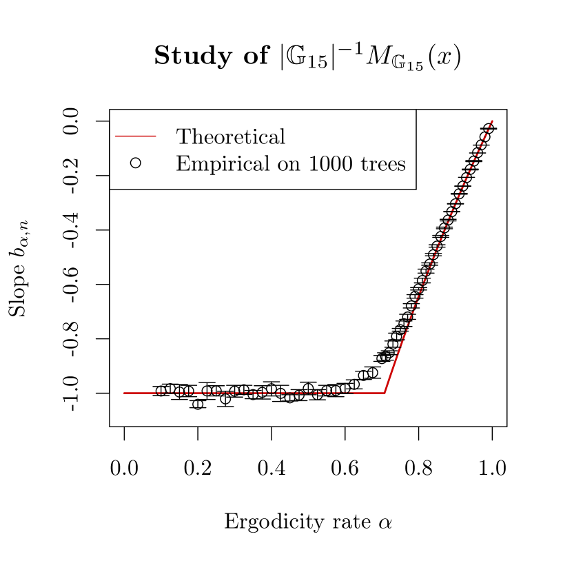
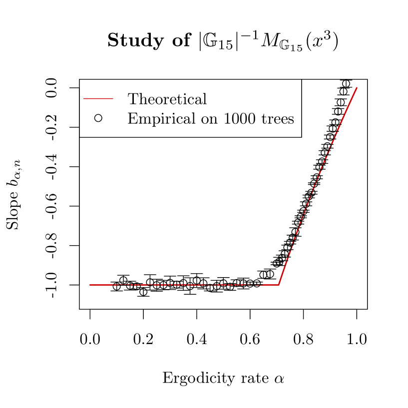
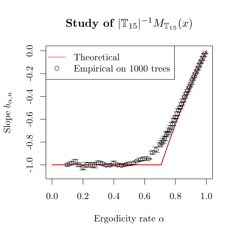
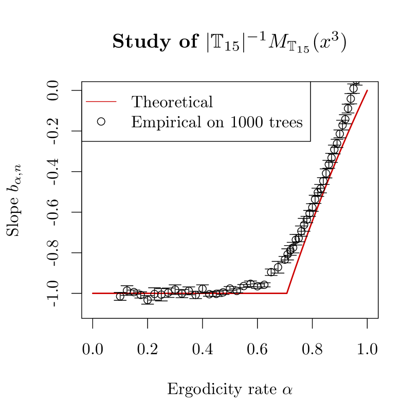
Figure 1. Slope $b_{\alpha,n}$ (empirical mean and confidence interval in black) of the regression line $\log({\mathrm{Var}}(|{\mathbb{A}}_{n}|^{-1}M_{{\mathbb{A}}_{n}}(f)))$ versus $\log(|{\mathbb{A}}_{n}|)$ as a function of the geometric ergodic rate $\alpha$, for $n=15$, ${\mathbb{A}}_{n}\in\{\mathbb{G}_{n},\mathbb{T}_{n}\}$ and $f(x)=x^{p}$ with $p\in\{1,3\}$. In this case, we have ${\mathcal{R}}(f)\neq 0$, where ${\mathcal{R}}$ is the projector defined from formula (31). One can see that the empirical curve (in black) is close to the graph (in red) of the function $h_{1}(\alpha)=\log(\alpha^{2}\vee 2^{-1})/\log(2)$ for $\alpha\in(0,1)$.

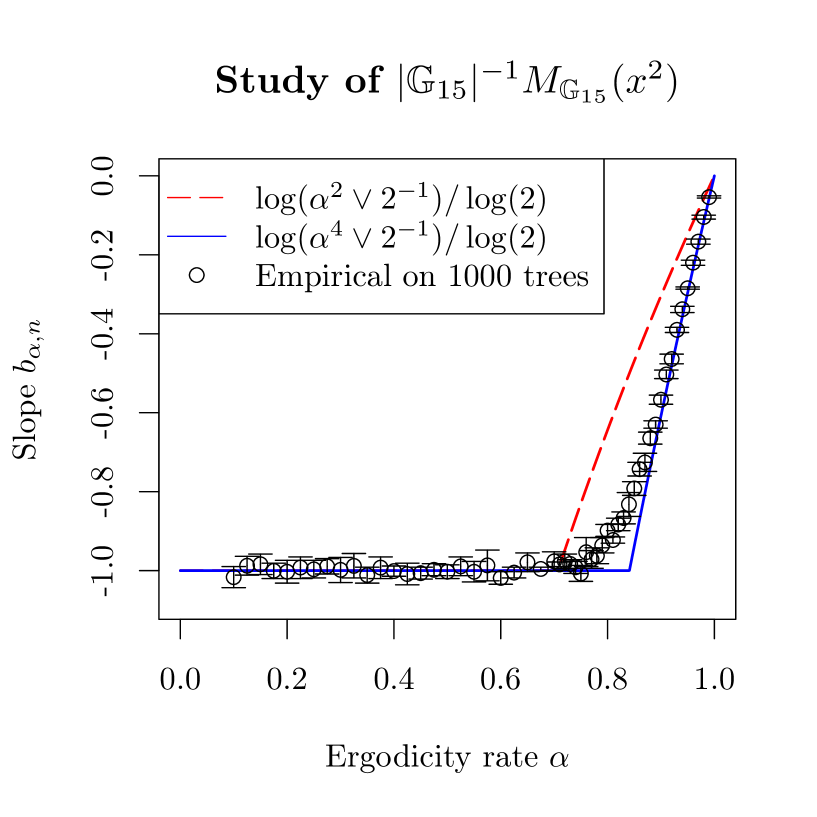
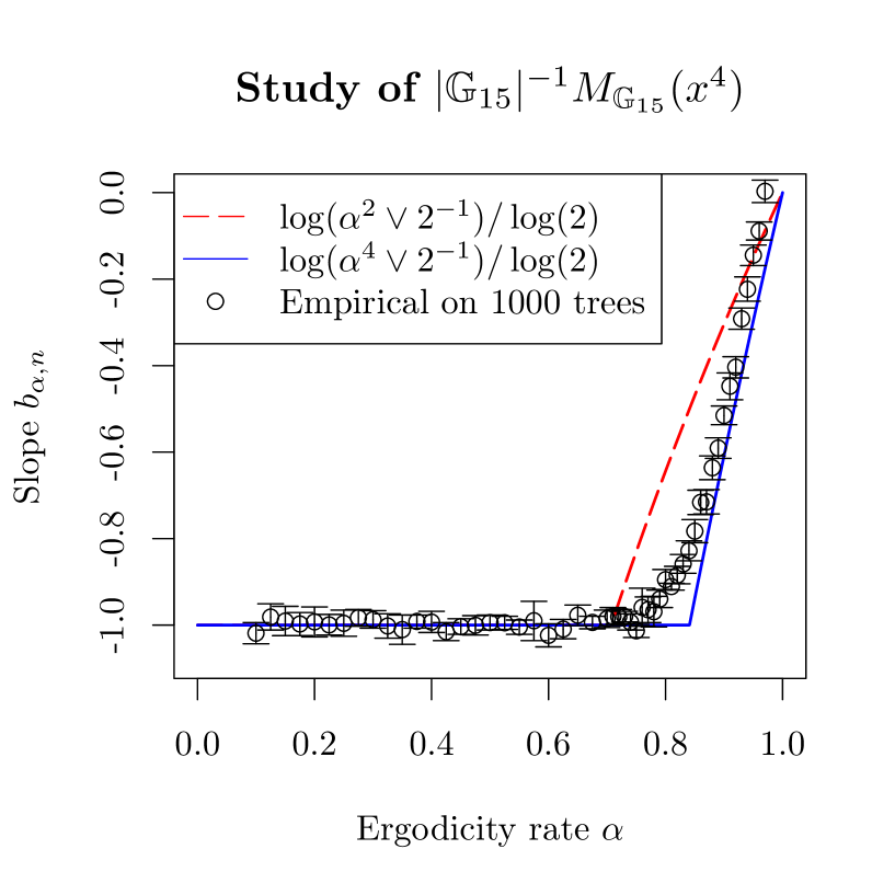
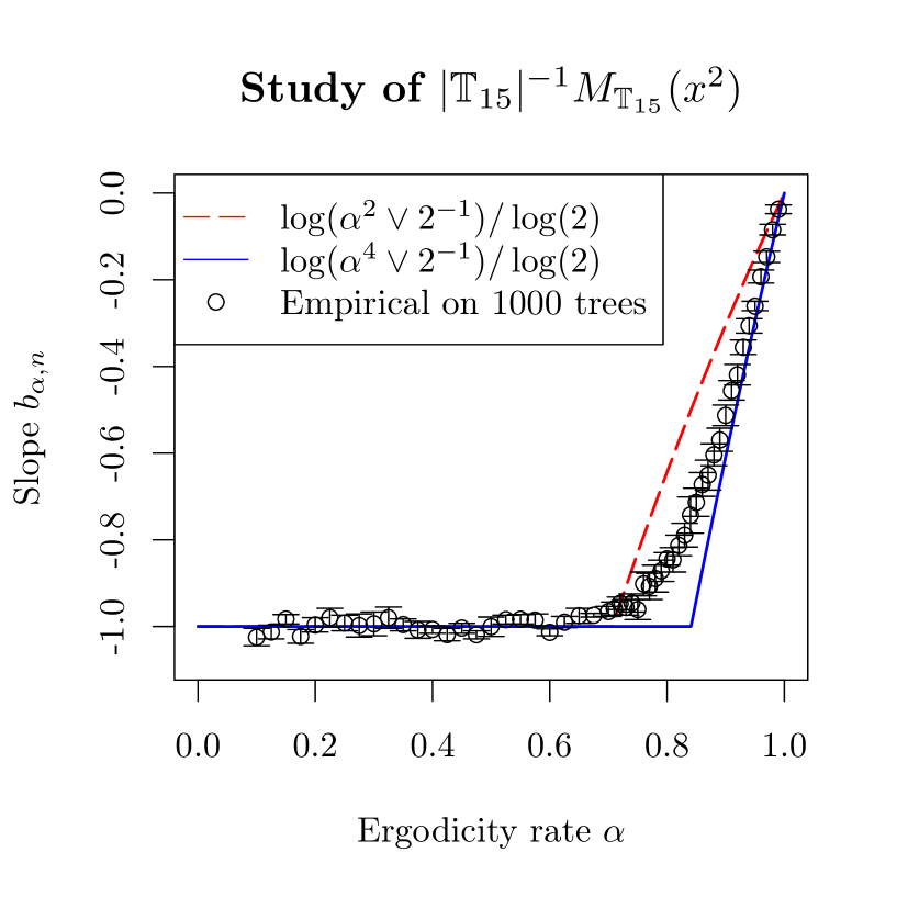
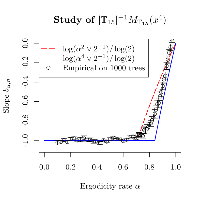
Figure 2. Slope $b_{\alpha,n}$ (empirical mean and confidence interval in black) of the regression line $\log({\mathrm{Var}}(|{\mathbb{A}}_{n}|^{-1}M_{{\mathbb{A}}_{n}}(f)))$ versus $\log(|{\mathbb{A}}_{n}|)$ as a function of the geometric ergodic rate $\alpha$, for $n=15$, ${\mathbb{A}}_{n}\in\{\mathbb{G}_{n},\mathbb{T}_{n}\}$ and $f(x)=x^{p}$ with $p\in\{2,4\}$. In this case, we have ${\mathcal{R}}(f)=0$, where ${\mathcal{R}}$ is the projector defined from formula (31). One can see that the empirical curve (in black) does not agree with the graph (dash line in red) of the function $h_{1}(\alpha)=\log(\alpha^{2}\vee 2^{-1})/\log(2)$ for $2\alpha^{2}>1$; but it is close to the graph (in blue) of the function $h_{2}(\alpha)=\log(\alpha^{4}\vee 2^{-1})/\log(2)$ for $\alpha\in(0,1)$.

5. Proof of Theorem 3.1

In the following proofs, we will denote by $C$ any unimportant finite constant which may vary from line to line (in particular $C$ does not depend on $n$ nor on ${\mathfrak{f}}$).

Let $(p_{n},n\in{\mathbb{N}})$ be a non-decreasing sequence of elements of ${\mathbb{N}}^{*}$ such that, for all $\lambda>0$:

(32) $$p_{n}<n,\quad\lim_{n\rightarrow\infty}p_{n}/n=1\quad\text{and}\quad\lim_{n\rightarrow\infty}n-p_{n}-\lambda\log(n)=+\infty.$$

When there is no ambiguity, we write $p$ for $p_{n}$.

Let $i,j\in\mathbb{T}$. We write $i\preccurlyeq j$ if $j\in i\mathbb{T}$. We denote by $i\wedge j$ the most recent common ancestor of $i$ and $j$, which is defined as the only $u\in\mathbb{T}$ such that if $v\in\mathbb{T}$ and $v\preccurlyeq i$, $v\preccurlyeq j$ then $v\preccurlyeq u$. We also define the lexicographic order $i\leq j$ if either $i\preccurlyeq j$ or $v0\preccurlyeq i$ and $v1\preccurlyeq j$ for $v=i\wedge j$. Let $X=(X_{i},i\in\mathbb{T})$ be a $BMC$ with kernel ${\mathcal{P}}$ and initial measure $\nu$. For $i\in\mathbb{T}$, we define the $\sigma$-field:

$${\mathcal{F}}_{i}=\{X_{u};u\in\mathbb{T}\text{ such that $u\leq i$}\}.$$

By construction, the $\sigma$-fields $({\mathcal{F}}_{i};\,i\in\mathbb{T})$ are nested as ${\mathcal{F}}_{i}\subset{\mathcal{F}}_{j}$ for $i\leq j$.

We define for $n\in{\mathbb{N}}$, $i\in\mathbb{G}_{n-p_{n}}$ and ${\mathfrak{f}}\in F^{\mathbb{N}}$ the martingale increments:

(33) $$\Delta_{n,i}({\mathfrak{f}})=N_{n,i}({\mathfrak{f}})-{\mathbb{E}}\left[N_{n,i}({\mathfrak{f}})|\,{\mathcal{F}}_{i}\right]\quad\text{and}\quad\Delta_{n}({\mathfrak{f}})=\sum_{i\in\mathbb{G}_{n-p_{n}}}\Delta_{n,i}({\mathfrak{f}}).$$

Thanks to (19), we have:

$$\sum_{i\in\mathbb{G}_{n-p_{n}}}N_{n,i}({\mathfrak{f}})=|\mathbb{G}_{n}|^{-1/2}\sum_{\ell=0}^{p_{n}}M_{\mathbb{G}_{n-\ell}}(\tilde{f}_{\ell})=|\mathbb{G}_{n}|^{-1/2}\sum_{k=n-p_{n}}^{n}M_{\mathbb{G}_{k}}(\tilde{f}_{n-k}).$$

Using the branching Markov property, and (19), we get for $i\in\mathbb{G}_{n-p_{n}}$:

$${\mathbb{E}}\left[N_{n,i}({\mathfrak{f}})|\,{\mathcal{F}}_{i}\right]={\mathbb{E}}\left[N_{n,i}({\mathfrak{f}})|\,X_{i}\right]=|\mathbb{G}_{n}|^{-1/2}\sum_{\ell=0}^{p_{n}}{\mathbb{E}}_{X_{i}}\left[M_{\mathbb{G}_{p_{n}-\ell}}(\tilde{f}_{\ell})\right].$$

We deduce from (21) with $k=n-p_{n}$ that:

(34) $$N_{n,\emptyset}({\mathfrak{f}})=\Delta_{n}({\mathfrak{f}})+R_{0}(n)+R_{1}(n),$$

with

(35) $$R_{0}(n)=|\mathbb{G}_{n}|^{-1/2}\,\sum_{k=0}^{n-p_{n}-1}M_{\mathbb{G}_{k}}(\tilde{f}_{n-k})\quad\text{and}\quad R_{1}(n)=\sum_{i\in\mathbb{G}_{n-p_{n}}}{\mathbb{E}}\left[N_{n,i}({\mathfrak{f}})|\,{\mathcal{F}}_{i}\right].$$

We first state a very useful Lemma which holds in sub-critical, critical and super-critical cases.

Lemma 5.1.

Let $X$ be a BMC with kernel ${\mathcal{P}}$ and initial distribution $\nu$ such that (ii) from Assumption 2.4 (with $k_{0}\in{\mathbb{N}}$) is in force. There exists a finite constant $C$, such that for all $f\in{\mathcal{B}}_{+}(S)$ all $n\geq k_{0}$, we have:

(36) $$|\mathbb{G}_{n}|^{-1}{\mathbb{E}}[M_{\mathbb{G}_{n}}(f)]\leq C\mathop{\parallel\!f\!\parallel}\nolimits_{L^{1}(\mu)}\quad\text{and}\quad|\mathbb{G}_{n}|^{-1}{\mathbb{E}}\left[M_{\mathbb{G}_{n}}(f)^{2}\right]\leq C\sum_{k=0}^{n}2^{k}\mathop{\parallel\!{\mathcal{Q}}^{k}f\!\parallel}\nolimits_{L^{2}(\mu)}^{2}.$$

Proof.

Using the first moment formula (73), (ii) from Assumption 2.4 and the fact that $\mu$ is invariant for ${\mathcal{Q}}$, we get that:

$$|\mathbb{G}_{n}|^{-1}{\mathbb{E}}[M_{\mathbb{G}_{n}}(f)]=\langle\nu,{\mathcal{Q}}^{n}f\rangle\leq\mathop{\parallel\!\nu_{0}\!\parallel}\nolimits_{\infty}\,\langle\mu,{\mathcal{Q}}^{n-k_{0}}f\rangle=\mathop{\parallel\!\nu_{0}\!\parallel}\nolimits_{\infty}\,\langle\mu,f\rangle.$$

We also have:

$$|\mathbb{G}_{n}|^{-1}{\mathbb{E}}\left[M_{\mathbb{G}_{n}}(f)^{2}\right] =\langle\nu,{\mathcal{Q}}^{n}(f^{2})\rangle+\sum_{k=0}^{n-1}2^{k}\,\langle\nu,{\mathcal{Q}}^{n-k-1}\left({\mathcal{P}}({\mathcal{Q}}^{k}f\otimes^{2}\right)\rangle$$

$$\leq\langle\nu,{\mathcal{Q}}^{n}(f^{2})\rangle+\sum_{k=0}^{n-1}2^{k}\,\langle\nu,{\mathcal{Q}}^{n-k}\left(({\mathcal{Q}}^{k}f)^{2}\right)\rangle$$

$$\leq\langle\nu,{\mathcal{Q}}^{n}(f^{2})\rangle+\sum_{k=0}^{n-k_{0}}2^{k}\,\langle\nu,{\mathcal{Q}}^{n-k}\left(({\mathcal{Q}}^{k}f)^{2}\right)\rangle+\sum_{k=n-k_{0}+1}^{n-1}2^{k}\,\langle\nu,{\mathcal{Q}}^{k_{0}}\left(({\mathcal{Q}}^{n-k_{0}}f)^{2}\right)\rangle$$

$$\leq C\sum_{k=0}^{n-k_{0}}2^{k}\mathop{\parallel\!{\mathcal{Q}}^{k}f\!\parallel}\nolimits_{L^{2}(\mu)}^{2},$$

where we used the second moment formula (74) for the equality, (3) for the first inequality, Jensen inequality for the second, and (ii) from Assumption 2.4 and the fact that $\mu$ is invariant for ${\mathcal{Q}}$ for the last. ∎

We set for $k\in{\mathbb{N}}^{*}$:

(37) $$c_{k}({\mathfrak{f}})=\sup_{n\in{\mathbb{N}}}\mathop{\parallel\!f_{n}\!\parallel}\nolimits_{L^{k}(\mu)}\quad\text{and}\quad q_{k}({\mathfrak{f}})=\sup_{n\in{\mathbb{N}}}\mathop{\parallel\!{\mathcal{Q}}(f_{n}^{k})\!\parallel}\nolimits_{\infty}^{1/k}.$$

We will denote by $C$ any unimportant finite constant which may vary from line to line (but in particular $C$ does not depend on $n$ nor on ${\mathfrak{f}}$, but may depends on $k_{0}$ and $\mathop{\parallel\!\nu_{0}\!\parallel}\nolimits_{\infty}$).

Remark 5.2.

Recall $k_{0}$ given in Assumption 2.4 (ii). Let ${\mathfrak{f}}=(f_{\ell},\ell\in\mathbb{N})$ be a bounded sequence in $L^{4}(\mu)$. We have

(38) $$N_{n,\emptyset}({\mathfrak{f}})=N_{n,\emptyset}^{[k_{0}]}({\mathfrak{f}})\,+\,|\mathbb{G}_{n}|^{-1/2}\sum_{\ell=0}^{k_{0}-1}M_{\mathbb{G}_{\ell}}(\tilde{f}_{n-\ell}),$$

where we set:

(39) $$\boxed{N_{n,\emptyset}^{[k_{0}]}({\mathfrak{f}})=|\mathbb{G}_{n}|^{-1/2}\sum_{\ell=0}^{n-k_{0}}M_{\mathbb{G}_{n-\ell}}(\tilde{f}_{\ell}).}$$

Using the Cauchy-Schwartz inequality, we get

(40) $$|\mathbb{G}_{n}|^{-1/2}|\sum_{\ell=0}^{k_{0}-1}M_{\mathbb{G}_{\ell}}(\tilde{f}_{n-\ell})|\leq Cc_{2}({\mathfrak{f}})|\mathbb{G}_{n}|^{-1/2}\,+\,|\mathbb{G}_{n}|^{-1/2}\sum_{\ell=0}^{k_{0}-1}M_{\mathbb{G}_{\ell}}(|f_{n-\ell}|).$$

Since the sequence ${\mathfrak{f}}$ is bounded in $L^{4}(\mu)$ and since $k_{0}$ is finite, we have, for all $\ell\in\{0,\ldots,k_{0}-1\}$, $\lim_{n\rightarrow\infty}|\mathbb{G}_{n}|^{-1/2}M_{\mathbb{G}_{\ell}}(|f_{n-\ell}|)=0$ a.s. and then that (used (40))

$$\lim_{n\rightarrow\infty}|\mathbb{G}_{n}|^{-1/2}|\sum_{\ell=0}^{k_{0}-1}M_{\mathbb{G}_{\ell}}(\tilde{f}_{n-\ell})|=0\quad\text{a.s.}$$

Therefore, from (38), the study of $N_{n,\emptyset}({\mathfrak{f}})$ is reduced to that of $N^{[k_{0}]}_{n,\emptyset}({\mathfrak{f}})$.

Recall $(p_{n},n\in{\mathbb{N}})$ is such that (32) holds. Assume that $n$ is large enough so that $n-p_{n}-1\geq k_{0}$. We have:

$$N^{[k_{0}]}_{n,\emptyset}({\mathfrak{f}})=\Delta_{n}({\mathfrak{f}})+R_{0}^{k_{0}}(n)+R_{1}(n),$$

where $\Delta_{n}({\mathfrak{f}})$ and $R_{1}(n)$ are defined in (33) and (35), and :

$$R_{0}^{k_{0}}(n)=|\mathbb{G}_{n}|^{-1/2}\,\sum_{k=k_{0}}^{n-p_{n}-1}M_{\mathbb{G}_{k}}(\tilde{f}_{n-k}).$$

Lemma 5.3.

Under the assumptions of Theorem 3.1, we have the following convergence:

$$\lim_{n\rightarrow\infty}{\mathbb{E}}[R_{0}^{k_{0}}(n)^{2}]=0.$$

Proof.

Assume $n-p\geq k_{0}$. We write:

$$R_{0}^{k_{0}}(n)=|\mathbb{G}_{n}|^{-1/2}\,\sum_{k=k_{0}}^{n-p-1}\sum_{i\in\mathbb{G}_{k_{0}}}M_{i\mathbb{G}_{k-k_{0}}}(\tilde{f}_{n-k}).$$

We have that $\sum_{i\in\mathbb{G}_{k_{0}}}{\mathbb{E}}[M_{i\mathbb{G}_{k-k_{0}}}(\tilde{f}_{n-k})^{2}]={\mathbb{E}}[M_{\mathbb{G}_{k_{0}}}(h_{k,n})]$, where:

$$h_{k,n}(x)={\mathbb{E}}_{x}[M_{\mathbb{G}_{k-k_{0}}}(\tilde{f}_{n-k})^{2}].$$

We deduce from (ii) from Assumption 2.4, see (36), that ${\mathbb{E}}[M_{\mathbb{G}_{k_{0}}}(h_{k,n})]\leq C\langle\mu,h_{k,n}\rangle$. We have also that:

$$\langle\mu,h_{k,n}\rangle={\mathbb{E}}_{\mu}[M_{\mathbb{G}_{k-k_{0}}}(\tilde{f}_{n-k})^{2}] \leq C\,2^{k}\sum_{\ell=0}^{k}2^{\ell}\mathop{\parallel\!{\mathcal{Q}}^{\ell}\tilde{f}_{n-k}\!\parallel}\nolimits_{L^{2}(\mu)}^{2}\leq C\,2^{k}\,c_{2}^{2}({\mathfrak{f}})\sum_{\ell=0}^{k}2^{\ell}\alpha^{2\ell}\leq C2^{k}\,c_{2}^{2}({\mathfrak{f}}),$$

where we used (36) for the first inequality (notice one can take $k_{0}=0$ in this case as we consider the expectation ${\mathbb{E}}_{\mu}$), (15) in the second, and $2\alpha^{2}<1$ in the last. We deduce that:

(41) $${\mathbb{E}}[R_{0}^{k_{0}}(n)^{2}]^{1/2}\leq|\mathbb{G}_{n}|^{-1/2}\,\sum_{k=k_{0}}^{n-p-1}\left(2^{k_{0}}{\mathbb{E}}\left[M_{\mathbb{G}_{k_{0}}}(h_{k,n})\right]\right)^{1/2}\leq C\,2^{-p/2}c_{2}({\mathfrak{f}}),$$

where we used that the sequence ${\mathfrak{f}}$ is bounded in $L^{2}(\mu)$. Use that $\lim_{n\rightarrow\infty}p=\infty$ to conclude. ∎

We have the following lemma.

Lemma 5.4.

Under the assumptions of Theorem 3.1, we have the following convergence:

$$\lim_{n\rightarrow\infty}{\mathbb{E}}\left[R_{1}(n)^{2}\right]=0.$$

Proof.

We set for $p\geq\ell\geq 0$, $n-p\geq k_{0}$ and $j\in\mathbb{G}_{k_{0}}$:

$$R_{1,j}(\ell,n)=\sum_{i\in j\mathbb{G}_{n-p-k_{0}}}{\mathbb{E}}\left[N_{n,i}^{\ell}(f_{\ell})|\,{\mathcal{F}}_{i}\right],$$

so that $R_{1}(n)=\sum_{\ell=0}^{p}\sum_{j\in\mathbb{G}_{k_{0}}}R_{1,j}(\ell,n)$. We have for $i\in\mathbb{G}_{n-p}$:

(42) $$|\mathbb{G}_{n}|^{1/2}{\mathbb{E}}\left[N_{n,i}^{\ell}(f_{\ell})|\,{\mathcal{F}}_{i}\right]={\mathbb{E}}\left[M_{i\mathbb{G}_{p-\ell}}(\tilde{f}_{\ell})|X_{i}\right]={\mathbb{E}}_{X_{i}}\left[M_{\mathbb{G}_{p-\ell}}(\tilde{f}_{\ell})\right]=|\mathbb{G}_{p-\ell}|\,{\mathcal{Q}}^{p-\ell}\tilde{f}_{\ell}(X_{i}),$$

where we used definition (18) of $N_{n,i}^{\ell}$ for the first equality, the Markov property of $X$ for the second and (73) for the third. Using (42), we get for $j\in\mathbb{G}_{k_{0}}$:

$$R_{1,j}(\ell,n)=|\mathbb{G}_{n}|^{-1/2}\,|\mathbb{G}_{p-\ell}|\,M_{j\mathbb{G}_{n-p-k_{0}}}({\mathcal{Q}}^{p-\ell}\tilde{f}_{\ell}).$$

We deduce from the Markov property of $X$ that ${\mathbb{E}}[R_{1,j}(\ell,n)^{2}|\,{\mathcal{F}}_{j}]=2^{-n+2(p-\ell)}\,h_{\ell,n}(X_{j})$ with $h_{\ell,n}(x)={\mathbb{E}}_{x}\left[M_{\mathbb{G}_{n-p-k_{0}}}({\mathcal{Q}}^{p-\ell}\tilde{f}_{\ell})^{2}\right]$. We have, thanks to (ii) from Assumption 2.4, see (36), that:

$$\sum_{j\in\mathbb{G}_{k_{0}}}{\mathbb{E}}[R_{1,j}(\ell,n)^{2}]=2^{-n+2(p-\ell)}\,{\mathbb{E}}\left[M_{\mathbb{G}_{k_{0}}}(h_{\ell,n})\right]\leq C2^{-n+2(p-\ell)}\,\langle\mu,h_{\ell,n}\rangle.$$

We have:

$$\langle\mu,h_{\ell,n}\rangle={\mathbb{E}}_{\mu}\left[M_{\mathbb{G}_{n-p-k_{0}}}({\mathcal{Q}}^{p-\ell}\tilde{f}_{\ell})^{2}\right] \leq C\,2^{n-p}\sum_{k=0}^{n-p-k_{0}}2^{k}\,\mathop{\parallel\!{\mathcal{Q}}^{k}{\mathcal{Q}}^{p-\ell}\tilde{f}_{\ell}\!\parallel}\nolimits_{L^{2}(\mu)}^{2}$$

$$\leq C\,2^{n-p}\alpha^{2(p-\ell)}\,c_{2}^{2}({\mathfrak{f}}),$$

where we used (36) for the first inequality (notice one can take $k_{0}=0$ in this case as we consider the expectation ${\mathbb{E}}_{\mu}$), (15) in the second, and $2\alpha^{2}<1$ in the last. We deduce that:

$$\sum_{j\in\mathbb{G}_{k_{0}}}{\mathbb{E}}\left[R_{1,j}(\ell,n)^{2}\right]\leq C\alpha^{2(p-\ell)}2^{p-2\ell}c_{2}^{2}({\mathfrak{f}}).$$

We get that:

$${\mathbb{E}}\left[R_{1}(n)^{2}\right]^{1/2}\leq\sum_{\ell=0}^{p}\left(2^{k_{0}}\sum_{j\in\mathbb{G}_{k_{0}}}{\mathbb{E}}\left[R_{1,j}(\ell,n)^{2}\right]\right)^{1/2}\leq C\,c_{2}({\mathfrak{f}})\,a_{1,n},$$

with the sequence $(a_{1,n},n\in{\mathbb{N}})$ defined by:

$$a_{1,n}=(2\alpha^{2})^{p/2}\sum_{\ell=0}^{p}(2\alpha)^{-\ell}.$$

The sequence $(a_{1,n},n\in{\mathbb{N}})$ does not depend on ${\mathfrak{f}}$ and converges to 0 since $\lim_{n\rightarrow\infty}p=\infty$, $2\alpha^{2}<1$ and

$$\sum_{\ell=0}^{p}(2\alpha)^{-\ell}\leq\begin{cases}2\alpha/(2\alpha-1)&\text{if $2\alpha>1$},\\ p+1&\text{if $2\alpha=1$},\\ (2\alpha)^{-p}/(1-2\alpha)&\text{if $2\alpha<1$}.\end{cases}$$

Then use that ${\mathfrak{f}}$ is bounded in $L^{2}(\mu)$ to conclude. ∎

Remark 5.5.

From the proofs of Lemmas 5.3 and 5.4, we have that $\mathbb{E}[(N_{n,\emptyset}^{[k_{0}]}({\mathfrak{f}})-\Delta_{n}({\mathfrak{f}}))^{2}]\leq a_{0,n}c_{2}({\mathfrak{f}})$, where the sequence $(a_{0,n},n\in\mathbb{N})$ converges to $0$ as $n$ goes to infinity.

We now study the bracket of $\Delta_{n}$:

$$V(n)=\sum_{i\in\mathbb{G}_{n-p_{n}}}{\mathbb{E}}\left[\Delta_{n,i}({\mathfrak{f}})^{2}|{\mathcal{F}}_{i}\right].$$

Using (19) and (33), we write:

(43) $$V(n)=|\mathbb{G}_{n}|^{-1}\sum_{i\in\mathbb{G}_{n-p_{n}}}{\mathbb{E}}_{X_{i}}\left[\left(\sum_{\ell=0}^{p_{n}}M_{\mathbb{G}_{p_{n}-\ell}}(\tilde{f}_{\ell})\right)^{2}\right]-R_{2}(n)=V_{1}(n)+2V_{2}(n)-R_{2}(n),$$

with:

$$V_{1}(n) =|\mathbb{G}_{n}|^{-1}\sum_{i\in\mathbb{G}_{n-p_{n}}}\sum_{\ell=0}^{p_{n}}{\mathbb{E}}_{X_{i}}\left[M_{\mathbb{G}_{p_{n}-\ell}}(\tilde{f}_{\ell})^{2}\right],$$

$$V_{2}(n) =|\mathbb{G}_{n}|^{-1}\sum_{i\in\mathbb{G}_{n-p_{n}}}\sum_{0\leq\ell<k\leq p_{n}}{\mathbb{E}}_{X_{i}}\left[M_{\mathbb{G}_{p_{n}-\ell}}(\tilde{f}_{\ell})M_{\mathbb{G}_{p_{n}-k}}(\tilde{f}_{k})\right],$$

$$R_{2}(n) =\sum_{i\in\mathbb{G}_{n-p_{n}}}{\mathbb{E}}\left[N_{n,i}({\mathfrak{f}})|X_{i}\right]^{2}.$$

Lemma 5.6.

Under the assumptions of Theorem 3.1, we have the following convergence:

$$\lim_{n\rightarrow\infty}{\mathbb{E}}\left[R_{2}(n)\right]=0.$$

Proof.

We define the sequence $(a_{2,n},n\in{\mathbb{N}})$ for $n\in{\mathbb{N}}$ by:

$$a_{2,n}=2^{-p}\left(\sum_{\ell=0}^{p}(2\alpha)^{\ell}\right)^{2}.$$

Notice that the sequence $(a_{2,n},n\in{\mathbb{N}})$ converges to 0 since $\lim_{n\rightarrow\infty}p=\infty$, $2\alpha^{2}<1$ and

$$\sum_{\ell=0}^{p}(2\alpha)^{\ell}\leq\begin{cases}(2\alpha)^{p+1}/(2\alpha-1)&\text{if $2\alpha>1$},\\ p+1&\text{if $2\alpha=1$},\\ 1/(1-2\alpha)&\text{if $2\alpha<1$}.\end{cases}$$

We now compute ${\mathbb{E}}_{x}\left[R_{2}(n)\right]$.

$${\mathbb{E}}_{x}\left[R_{2}(n)\right] =|\mathbb{G}_{n}|^{-1}\,\sum_{i\in\mathbb{G}_{n-p}}{\mathbb{E}}_{x}\left[{\mathbb{E}}_{x}\left[\sum_{\ell=0}^{p}M_{i\mathbb{G}_{p-\ell}}(\tilde{f}_{\ell})|X_{i}\right]^{2}\right]$$

$$=|\mathbb{G}_{n}|^{-1}\,\sum_{i\in\mathbb{G}_{n-p}}{\mathbb{E}}_{x}\left[\left(\sum_{\ell=0}^{p}{\mathbb{E}}_{X_{i}}\left[M_{\mathbb{G}_{p-\ell}}(\tilde{f}_{\ell})\right]\right)^{2}\right].$$

$$=|\mathbb{G}_{n}|^{-1}\,|\mathbb{G}_{n-p}|\,{\mathcal{Q}}^{n-p}\left(\Big{(}\sum_{\ell=0}^{p}|\mathbb{G}_{p-\ell}|\,{\mathcal{Q}}^{p-\ell}\tilde{f}_{\ell}\Big{)}^{2}\right)(x)$$

where we used the definition of $N_{n,i}({\mathfrak{f}})$ for the first equality, the Markov property of $X$ for the second, (73) for the third. From the latter equality, we have using (ii) from Assumption 2.4:

$${\mathbb{E}}\left[R_{2}(n)\right] =|\mathbb{G}_{n}|^{-1}\,|\mathbb{G}_{n-p}|\,\langle\nu,{\mathcal{Q}}^{n-p}\left(\Big{(}\sum_{\ell=0}^{p}|\mathbb{G}_{p-\ell}|\,{\mathcal{Q}}^{p-\ell}\tilde{f}_{\ell}\Big{)}^{2}\right)\rangle$$

$$\leq C2^{-p}\left(\sum_{\ell=0}^{p}|\mathbb{G}_{p-\ell}|\,\mathop{\parallel\!{\mathcal{Q}}^{p-\ell}\tilde{f}_{\ell}\!\parallel}\nolimits_{L^{2}(\mu)}\right)^{2}.$$

We deduce that:

$${\mathbb{E}}\left[R_{2}(n)\right]\leq C\,c_{2}^{2}({\mathfrak{f}})\,a_{2,n},$$

Then use that ${\mathfrak{f}}$ is bounded in $L^{2}(\mu)$ to conclude. ∎

Remark 5.7.

In particular, we have obtained from the previous proof that $\mathbb{E}[|V(n)-V_{1}(n)-V_{2}(n)|]\leq Cc_{2}^{2}({\mathfrak{f}})a_{2,n}$, with the sequence $(a_{2,n},n\in\mathbb{N})$ going to 0 as $n$ goes to infinity.

Lemma 5.8.

Under the assumptions of Theorem 3.1, we have that in probability $\lim_{n\rightarrow\infty}V_{2}(n)=\Sigma^{\rm sub}_{2}({\mathfrak{f}})$ with $\Sigma^{\rm sub}_{2}({\mathfrak{f}})$ finite and defined in (24).

Proof.

Using (75), we get:

(44) $$V_{2}(n)=V_{5}(n)+V_{6}(n),$$

with

$$V_{5}(n) =|\mathbb{G}_{n}|^{-1}\sum_{i\in\mathbb{G}_{n-p}}\sum_{0\leq\ell<k\leq p}2^{p-\ell}{\mathcal{Q}}^{p-k}\left(\tilde{f}_{k}{\mathcal{Q}}^{k-\ell}\tilde{f}_{\ell}\right)(X_{i}),$$

$$V_{6}(n) =|\mathbb{G}_{n}|^{-1}\sum_{i\in\mathbb{G}_{n-p}}\sum_{0\leq\ell<k<p}\sum_{r=0}^{p-k-1}2^{p-\ell+r}\,{\mathcal{Q}}^{p-1-(r+k)}\left({\mathcal{P}}\left({\mathcal{Q}}^{r}\tilde{f}_{k}\otimes_{\rm sym}{\mathcal{Q}}^{k-\ell+r}\tilde{f}_{\ell}\right)\right)(X_{i}).$$

We consider the term $V_{6}(n)$. We have:

$$V_{6}(n)=|\mathbb{G}_{n-p}|^{-1}M_{\mathbb{G}_{n-p}}(H_{6,n}),$$

with:

(45) $$H_{6,n}=\sum_{\begin{subarray}{c}0\leq\ell<k\\ r\geq 0\end{subarray}}h_{k,\ell,r}^{(n)}\,{\bf 1}_{\{r+k<p\}}\quad\text{and}\quad h_{k,\ell,r}^{(n)}=2^{r-\ell}\,{\mathcal{Q}}^{p-1-(r+k)}\left({\mathcal{P}}\left({\mathcal{Q}}^{r}\tilde{f}_{k}\otimes_{\rm sym}{\mathcal{Q}}^{k-\ell+r}\tilde{f}_{\ell}\right)\right).$$

Define $H_{6}({\mathfrak{f}})=\sum_{0\leq\ell<k;r\geq 0}h_{k,\ell,r}$ with $h_{k,\ell,r}=2^{r-\ell}\langle\mu,{\mathcal{P}}\left({\mathcal{Q}}^{r}\tilde{f}_{k}\otimes_{\rm sym}{\mathcal{Q}}^{k-\ell+r}\tilde{f}_{\ell}\right)\rangle=\langle\mu,h_{k,\ell,r}^{(n)}\rangle$. Thanks to (5) and (15), we get that:

(46) $$|h_{k,\ell,r}|\leq C\,2^{r-\ell}\mathop{\parallel\!{\mathcal{Q}}^{r}\tilde{f}_{k}\!\parallel}\nolimits_{L^{2}(\mu)}\mathop{\parallel\!{\mathcal{Q}}^{k-\ell+r}\tilde{f}_{\ell}\!\parallel}\nolimits_{L^{2}(\mu)}\leq C\,2^{r-\ell}\alpha^{k-\ell+2r}\mathop{\parallel\!f_{\ell}\!\parallel}\nolimits_{L^{2}(\mu)}\mathop{\parallel\!f_{k}\!\parallel}\nolimits_{L^{2}(\mu)}.$$

We deduce that $|h_{k,\ell,r}|\leq C\,2^{r-\ell}\alpha^{k-\ell+2r}c_{2}^{2}({\mathfrak{f}})$ and, as the sum $\sum_{0\leq\ell<k,\,r\geq 0}2^{r-\ell}\alpha^{k-\ell+2r}$ is finite:

(47) $$|H_{6}({\mathfrak{f}})|\leq C\,c_{2}^{2}({\mathfrak{f}}).$$

We write $H_{6}({\mathfrak{f}})=H_{6}^{[n]}({\mathfrak{f}})+B_{6,n}({\mathfrak{f}})$, with

$$H_{6}^{[n]}({\mathfrak{f}})=\sum_{\begin{subarray}{c}0\leq\ell<k\\ r\geq 0\end{subarray}}h_{k,\ell,r}\,{\bf 1}_{\{r+k<p\}}\quad\text{and}\quad B_{6,n}({\mathfrak{f}})=\sum_{\begin{subarray}{c}0\leq\ell<k\\ r\geq 0\end{subarray}}h_{k,\ell,r}\,{\bf 1}_{\{r+k\geq p\}}.$$

As $\lim_{n\rightarrow\infty}{\bf 1}_{\{r+k\geq p\}}=0$, we get from (46), (47) and dominated convergence that $\lim_{n\rightarrow\infty}B_{6,n}({\mathfrak{f}})=0$ and thus:

(48) $$\lim_{n\rightarrow\infty}H_{6}^{[n]}({\mathfrak{f}})=H_{6}({\mathfrak{f}}).$$

We set $A_{6,n}({\mathfrak{f}})=H_{6,n}-H_{6}^{[n]}({\mathfrak{f}})=\sum_{\begin{subarray}{c}0\leq\ell<k\\ r\geq 0\end{subarray}}(h_{k,\ell,r}^{(n)}-h_{k,\ell,r})\,{\bf 1}_{\{r+k<p\}}$, so that from the definition of $V_{6}(n)$, we get that:

$$V_{6}(n)-H_{6}^{[n]}({\mathfrak{f}})=|\mathbb{G}_{n-p}|^{-1}\,M_{\mathbb{G}_{n-p}}(A_{6,n}({\mathfrak{f}})).$$

We now study the second moment of $|\mathbb{G}_{n-p}|^{-1}\,M_{\mathbb{G}_{n-p}}(A_{6,n}({\mathfrak{f}}))$. Using (36), we get for $n-p\geq k_{0}$:

$$|\mathbb{G}_{n-p}|^{-2}\,{\mathbb{E}}\left[M_{\mathbb{G}_{n-p}}(A_{6,n}({\mathfrak{f}}))^{2}\right]\leq C\,|\mathbb{G}_{n-p}|^{-1}\,\sum_{j=0}^{n-p}2^{j}\mathop{\parallel\!{\mathcal{Q}}^{j}(A_{6,n}({\mathfrak{f}}))\!\parallel}\nolimits_{L^{2}(\mu)}^{2}.$$

Recall $c_{k}({\mathfrak{f}})$ and $q_{k}({\mathfrak{f}})$ from (37). We deduce that

$$\mathop{\parallel\!{\mathcal{Q}}^{j}(A_{6,n}({\mathfrak{f}}))\!\parallel}\nolimits_{L^{2}(\mu)} \leq\sum_{\begin{subarray}{c}0\leq\ell<k\\ r\geq 0\end{subarray}}\mathop{\parallel\!{\mathcal{Q}}^{j}h_{k,\ell,r}^{(n)}-h_{k,\ell,r}\!\parallel}\nolimits_{L^{2}(\mu)}{\bf 1}_{\{r+k<p\}}$$

$$\leq C\sum_{\begin{subarray}{c}0\leq\ell<k\\ r\geq 0\end{subarray}}2^{r-\ell}\,\alpha^{p-1-(r+k)+j}\mathop{\parallel\!{\mathcal{P}}\left({\mathcal{Q}}^{r}\tilde{f}_{k}\otimes_{\rm sym}{\mathcal{Q}}^{k-\ell+r}\tilde{f}_{\ell}\right)\!\parallel}\nolimits_{L^{2}(\mu)}{\bf 1}_{\{r+k<p\}}$$

$$\leq Cc_{2}^{2}({\mathfrak{f}})\,\alpha^{j}\,\sum_{\begin{subarray}{c}0\leq\ell<k\\ r\geq 1\end{subarray}}2^{r-\ell}\,\alpha^{p-(r+k)}\alpha^{k-\ell+2r}\,{\bf 1}_{\{r+k<p\}}$$

$$\hskip 56.9055pt+C\alpha^{j}\,\sum_{0\leq\ell<k}2^{-\ell}\,\alpha^{p-k}\mathop{\parallel\!{\mathcal{P}}\left(\tilde{f}_{k}\otimes_{\rm sym}{\mathcal{Q}}^{k-\ell}\tilde{f}_{\ell}\right)\!\parallel}\nolimits_{L^{2}(\mu)}\,{\bf 1}_{\{k<p\}}$$

$$\leq Cc_{2}({\mathfrak{f}})c_{4}({\mathfrak{f}})\,\alpha^{j}\,\sum_{\begin{subarray}{c}0\leq\ell<k\\ r\geq 0\end{subarray}}2^{r-\ell}\,\alpha^{p-(r+k)}\alpha^{k-\ell+2r}\,{\bf 1}_{\{r+k<p\}}$$

$$\leq Cc_{2}({\mathfrak{f}})c_{4}({\mathfrak{f}})\,\alpha^{j},$$

where we used the triangular inequality for the first inequality; (15) for the second; (6) for $r\geq 1$ and (15) again for the third; (8) for $r=0$ to get the $c_{4}({\mathfrak{f}})$ term and $c_{2}({\mathfrak{f}})\leq c_{4}({\mathfrak{f}})$ for the fourth; and that $\sum_{{0\leq\ell<k,\,r\geq 0}}2^{r-\ell}\alpha^{k-\ell+2r}$ is finite for the last. As $\sum_{j=0}^{\infty}(2\alpha^{2})^{j}$ is finite, we deduce that:

(49) $${\mathbb{E}}\left[\left(V_{6}(n)-H_{6}^{[n]}({\mathfrak{f}})\right)^{2}\right]=|\mathbb{G}_{n-p}|^{-2}\,{\mathbb{E}}\left[M_{\mathbb{G}_{n-p}}(A_{6,n}({\mathfrak{f}}))^{2}\right]\leq Cc_{2}^{2}({\mathfrak{f}})c_{4}^{2}({\mathfrak{f}})\,2^{-(n-p)}.$$

We now consider the term $V_{5}(n)$ defined just after (44):

$$V_{5}(n)=|\mathbb{G}_{n-p}|^{-1}M_{\mathbb{G}_{n-p}}(H_{5,n}),$$

with

$$H_{5,n}=\sum_{0\leq\ell<k}h_{k,\ell}^{(n)}\,{\bf 1}_{\{k\leq p\}}\quad\text{and}\quad h_{k,\ell}^{(n)}=2^{-\ell}\,{\mathcal{Q}}^{p-k}\left(\tilde{f}_{k}{\mathcal{Q}}^{k-\ell}\tilde{f}_{\ell}\right).$$

Define $H_{5}({\mathfrak{f}})=\sum_{0\leq\ell<k}h_{k,\ell}$ with $h_{k,\ell}=2^{-\ell}\langle\mu,\tilde{f}_{k}{\mathcal{Q}}^{k-\ell}\tilde{f}_{\ell}\rangle$. We have using Cauchy-Schwartz inequality and (15) that:

(50) $$|h_{k,\ell}|\leq C\,2^{-\ell}\alpha^{k-\ell}\mathop{\parallel\!f_{\ell}\!\parallel}\nolimits_{L^{2}(\mu)}\mathop{\parallel\!f_{k}\!\parallel}\nolimits_{L^{2}(\mu)}\leq C\,2^{-\ell}\alpha^{k-\ell}\,c_{2}^{2}({\mathfrak{f}}).$$

As the sum $\sum_{0\leq\ell<k}2^{-\ell}\alpha^{k-\ell}$ is finite, we deduce that:

(51) $$|H_{5}({\mathfrak{f}})|\leq C\,c_{2}^{2}({\mathfrak{f}}).$$

We write $H_{5}({\mathfrak{f}})=H_{5}^{[n]}({\mathfrak{f}})+B_{5,n}({\mathfrak{f}})$, with

(52) $$H_{5}^{[n]}({\mathfrak{f}})=\!\!\sum_{0\leq\ell<k}\!\!h_{k,\ell}{\bf 1}_{\{k\leq p\}}=\!\!\sum_{0\leq\ell<k}\!\!2^{-\ell}\langle\mu,\tilde{f}_{k}{\mathcal{Q}}^{k-\ell}\tilde{f}_{\ell}\rangle{\bf 1}_{\{k\leq p\}}\quad\text{and}\quad B_{5,n}({\mathfrak{f}})=\!\!\sum_{0\leq\ell<k}\!\!h_{k,\ell}\,{\bf 1}_{\{k>p\}}.$$

As $\lim_{n\rightarrow\infty}{\bf 1}_{\{k>p\}}=0$, we deduce from (50) and (51) that $\lim_{n\rightarrow\infty}B_{5,n}({\mathfrak{f}})=0$ by dominated convergence and thus:

(53) $$\lim_{n\rightarrow\infty}H_{5}^{[n]}({\mathfrak{f}})=H_{5}({\mathfrak{f}}).$$

We set $A_{5,n}({\mathfrak{f}})=H_{5,n}-H_{5}^{[n]}({\mathfrak{f}})=\sum_{0\leq\ell<k}(h_{k,\ell}^{(n)}-h_{k,\ell})\,{\bf 1}_{\{k\leq p\}}$, so that from the definition of $V_{5}(n)$, we get that:

(54) $$V_{5}(n)-H_{5}^{[n]}({\mathfrak{f}})=|\mathbb{G}_{n-p}|^{-1}\,M_{\mathbb{G}_{n-p}}(A_{5,n}({\mathfrak{f}})).$$

We now study the second moment of $|\mathbb{G}_{n-p}|^{-1}\,M_{\mathbb{G}_{n-p}}(A_{5,n}({\mathfrak{f}}))$. Using (36), we get for $n-p\geq k_{0}$:

$$|\mathbb{G}_{n-p}|^{-2}\,{\mathbb{E}}\left[M_{\mathbb{G}_{n-p}}(A_{5,n}({\mathfrak{f}}))^{2}\right]\leq C\,|\mathbb{G}_{n-p}|^{-1}\,\sum_{j=0}^{n-p}2^{j}\mathop{\parallel\!{\mathcal{Q}}^{j}(A_{5,n}({\mathfrak{f}}))\!\parallel}\nolimits_{L^{2}(\mu)}^{2}.$$

We also have that:

$$\mathop{\parallel\!{\mathcal{Q}}^{j}(A_{5,n}({\mathfrak{f}}))\!\parallel}\nolimits_{L^{2}(\mu)} \leq\sum_{0\leq\ell<k}\mathop{\parallel\!{\mathcal{Q}}^{j}h_{k,\ell}^{(n)}-h_{k,\ell}\!\parallel}\nolimits_{L^{2}(\mu)}{\bf 1}_{\{k\leq p\}}$$

$$\leq C\sum_{0\leq\ell<k}2^{-\ell}\,\alpha^{p-k+j}\mathop{\parallel\!\tilde{f}_{k}{\mathcal{Q}}^{k-\ell}\tilde{f}_{\ell}\!\parallel}\nolimits_{L^{2}(\mu)}{\bf 1}_{\{k\leq p\}}$$

(55) $$\leq Cc_{4}^{2}({\mathfrak{f}})\,\alpha^{j},$$

where we used the triangular inequality for the first inequality, (15) for the second, and Cauchy-Schwartz inequality for the last. As $\sum_{j=0}^{\infty}(2\alpha^{2})^{j}$ is finite, we deduce that:

(56) $${\mathbb{E}}\left[\left(V_{5}(n)-H_{5}^{[n]}({\mathfrak{f}})\right)^{2}\right]=|\mathbb{G}_{n-p}|^{-2}\,{\mathbb{E}}\left[M_{\mathbb{G}_{n-p}}(A_{5,n}({\mathfrak{f}}))^{2}\right]\leq C\,c_{4}^{4}({\mathfrak{f}})\,2^{-(n-p)}.$$

Since $c_{2}({\mathfrak{f}})\leq c_{4}({\mathfrak{f}})$, we deduce from (49) and (56), as $V_{2}(n)=V_{5}(n)+V_{6}(n)$ (see (44)), that:

$${\mathbb{E}}\left[\left(V_{2}(n)-H_{2}^{[n]}({\mathfrak{f}})\right)^{2}\right]\leq C\,c_{4}^{4}({\mathfrak{f}})\,2^{-(n-p)}\quad\text{with}\quad H_{2}^{[n]}({\mathfrak{f}})=H_{6}^{[n]}({\mathfrak{f}})+H_{5}^{[n]}({\mathfrak{f}}).$$

Since, according to (48) and (53) and $\Sigma^{\rm sub}_{2}({\mathfrak{f}})=H_{6}({\mathfrak{f}})+H_{5}({\mathfrak{f}})$ (see (24)), we get $\lim_{n\rightarrow\infty}H_{2}^{[n]}({\mathfrak{f}})=\Sigma^{\rm sub}_{2}({\mathfrak{f}})$. This implies that $\lim_{n\rightarrow\infty}V_{2}(n)=\Sigma^{\rm sub}_{2}({\mathfrak{f}})$ in probability.

∎

We now study the limit of $V_{1}(n)$.

Lemma 5.9.

Under the assumptions of Theorem 3.1, we have that in probability $\lim_{n\rightarrow\infty}V_{1}(n)=\Sigma^{\rm sub}_{1}({\mathfrak{f}})<+\infty$ with $\Sigma^{\rm sub}_{1}({\mathfrak{f}})$ finite and defined in (23).

Proof.

Using (74), we get:

(57) $$V_{1}(n)=V_{3}(n)+V_{4}(n),$$

with

$$V_{3}(n) =|\mathbb{G}_{n}|^{-1}\sum_{i\in\mathbb{G}_{n-p}}\sum_{\ell=0}^{p}2^{p-\ell}\,{\mathcal{Q}}^{p-\ell}(\tilde{f}_{\ell}^{2})(X_{i}),$$

$$V_{4}(n) =|\mathbb{G}_{n}|^{-1}\sum_{i\in\mathbb{G}_{n-p}}\sum_{\ell=0}^{p-1}\,\sum_{k=0}^{p-\ell-1}2^{p-\ell+k}\,{\mathcal{Q}}^{p-1-(\ell+k)}\left({\mathcal{P}}\left({\mathcal{Q}}^{k}\tilde{f}_{\ell}\otimes^{2}\right)\right)(X_{i}).$$

We first consider the term $V_{4}(n)$. We have:

$$V_{4}(n)=|\mathbb{G}_{n-p}|^{-1}M_{\mathbb{G}_{n-p}}(H_{4,n}),$$

with:

$$H_{4,n}=\sum_{\ell\geq 0,\,k\geq 0}h_{\ell,k}^{(n)}\,{\bf 1}_{\{\ell+k<p\}}\quad\text{and}\quad h_{\ell,k}^{(n)}=2^{k-\ell}\,{\mathcal{Q}}^{p-1-(\ell+k)}\left({\mathcal{P}}\left({\mathcal{Q}}^{k}\tilde{f}_{\ell}\otimes^{2}\right)\right).$$

Define the constant $H_{4}({\mathfrak{f}})=\sum_{\ell\geq 0,\,k\geq 0}h_{\ell,k}$ with $h_{\ell,k}=2^{k-\ell}\,\langle\mu,{\mathcal{P}}\left({\mathcal{Q}}^{k}\tilde{f}_{\ell}\otimes^{2}\right)\rangle$. Thanks to (3) and (15), we have:

(58) $$|h_{\ell,k}|\leq 2^{k-\ell}\mathop{\parallel\!{\mathcal{Q}}^{k}\tilde{f}_{\ell}\!\parallel}\nolimits_{L^{2}(\mu)}^{2}\leq C\,2^{k-\ell}\alpha^{2k}\mathop{\parallel\!f_{\ell}\!\parallel}\nolimits_{L^{2}(\mu)}^{2}\leq C\,2^{k-\ell}\alpha^{2k}\,c_{2}^{2}({\mathfrak{f}}),$$

and thus, as the sum $\sum_{\ell\geq 0,\,k\geq 0}2^{k-\ell}\alpha^{2k}$ is finite:

(59) $$|H_{4}({\mathfrak{f}})|\leq C\,c_{2}^{2}({\mathfrak{f}}).$$

We write $H_{4}({\mathfrak{f}})=H_{4}^{[n]}({\mathfrak{f}})+B_{4,n}({\mathfrak{f}})$, with

$$H_{4}^{[n]}({\mathfrak{f}})=\sum_{\ell\geq 0,\,k\geq 0}h_{\ell,k}\,{\bf 1}_{\{\ell+k<p\}}\quad\text{and}\quad B_{4,n}({\mathfrak{f}})=\sum_{\ell\geq 0,\,k\geq 0}h_{\ell,k}\,{\bf 1}_{\{\ell+k\geq p\}}.$$

Using that $\lim_{n\rightarrow\infty}{\bf 1}_{\{\ell+k\geq p\}}=0$, we deduce from (58), (59) and dominated convergence that $\lim_{n\rightarrow\infty}B_{4,n}({\mathfrak{f}})=0$, and thus:

(60) $$\lim_{n\rightarrow\infty}H_{4}^{[n]}({\mathfrak{f}})=H_{4}({\mathfrak{f}}).$$

We set $A_{4,n}({\mathfrak{f}})=H_{4,n}-H_{4}^{[n]}({\mathfrak{f}})=\sum_{\ell\geq 0,\,k\geq 0}(h_{\ell,k}^{(n)}-h_{\ell,k})\,{\bf 1}_{\{\ell+k<p\}}$, so that from the definition of $V_{4}(n)$, we get that:

$$V_{4}(n)-H_{4}^{[n]}({\mathfrak{f}})=|\mathbb{G}_{n-p}|^{-1}\,M_{\mathbb{G}_{n-p}}(A_{4,n}({\mathfrak{f}})).$$

We now study the second moment of $|\mathbb{G}_{n-p}|^{-1}\,M_{\mathbb{G}_{n-p}}(A_{4,n}({\mathfrak{f}}))$. Using (36), we get for $n-p\geq k_{0}$:

$$|\mathbb{G}_{n-p}|^{-2}\,{\mathbb{E}}\left[M_{\mathbb{G}_{n-p}}(A_{4,n}({\mathfrak{f}}))^{2}\right]\leq C\,|\mathbb{G}_{n-p}|^{-1}\,\sum_{j=0}^{n-p}2^{j}\mathop{\parallel\!{\mathcal{Q}}^{j}(A_{4,n}({\mathfrak{f}}))\!\parallel}\nolimits_{L^{2}(\mu)}^{2}.$$

Using (3), we obtain that $\mathop{\parallel\!{\mathcal{P}}(\tilde{f}_{\ell}\otimes\tilde{f}_{\ell})\!\parallel}\nolimits_{L^{2}(\mu)}\leq c_{4}^{2}({\mathfrak{f}})$. We deduce that:

$$\mathop{\parallel\!{\mathcal{Q}}^{j}(A_{4,n}({\mathfrak{f}}))\!\parallel}\nolimits_{L^{2}(\mu)} \leq\sum_{\ell\geq 0,\,k\geq 0}\mathop{\parallel\!{\mathcal{Q}}^{j}h_{\ell,k}^{(n)}-h_{\ell,k}\!\parallel}\nolimits_{L^{2}(\mu)}{\bf 1}_{\{\ell+k<p\}}$$

$$\leq C\sum_{\ell\geq 0,\,k\geq 0}2^{k-\ell}\,\alpha^{p-1-(\ell+k)+j}\mathop{\parallel\!{\mathcal{P}}\left({\mathcal{Q}}^{k}\tilde{f}_{\ell}\otimes^{2}\right)\!\parallel}\nolimits_{L^{2}(\mu)}{\bf 1}_{\{\ell+k<p\}}$$

$$\leq C\,c_{2}^{2}({\mathfrak{f}})\,\alpha^{j}\!\!\!\sum_{\ell\geq 0,\,k>0}\!\!\!2^{k-\ell}\,\alpha^{p-(\ell+k)}\alpha^{2k}\,{\bf 1}_{\{\ell+k<p\}}$$

$$\hskip 56.9055pt+C\,\alpha^{j}\sum_{\ell\geq 0}2^{-\ell}\,\alpha^{p-\ell}\mathop{\parallel\!{\mathcal{P}}\left(\tilde{f}_{\ell}\otimes^{2}\right)\!\parallel}\nolimits_{L^{2}(\mu)}{\bf 1}_{\{\ell<p\}}$$

$$\leq C\,c_{4}^{2}({\mathfrak{f}})\,\alpha^{j},$$

where we used the triangular inequality for the first inequality; (15) for the second; (6) for $k\geq 1$ and (15) again for the third; and (3) as well as $c_{2}({\mathfrak{f}})\leq c_{4}({\mathfrak{f}})$ for the last. As $\sum_{j=0}^{\infty}(2\alpha^{2})^{j}$ is finite, we deduce that:

(61) $${\mathbb{E}}\left[\left(V_{4}(n)-H_{4}^{[n]}({\mathfrak{f}})\right)^{2}\right]=|\mathbb{G}_{n-p}|^{-2}\,{\mathbb{E}}\left[M_{\mathbb{G}_{n-p}}(A_{4,n}({\mathfrak{f}}))^{2}\right]\leq C\,c_{4}^{4}({\mathfrak{f}})\,2^{-(n-p)}.$$

We now consider the term $V_{3}(n)$ defined just after (57):

$$V_{3}(n)=|\mathbb{G}_{n-p}|^{-1}M_{\mathbb{G}_{n-p}}(H_{3,n}),$$

with

$$H_{3,n}=\sum_{\ell\geq 0}h_{\ell}^{(n)}\,{\bf 1}_{\{\ell\leq p\}}\quad\text{and}\quad h_{\ell}^{(n)}=2^{-\ell}\,{\mathcal{Q}}^{p-\ell}\left(\tilde{f}_{\ell}^{2}\right).$$

Define the constant $H_{3}({\mathfrak{f}})=\sum_{\ell\geq 0}h_{\ell}$ with $h_{\ell}=2^{-\ell}\langle\mu,\tilde{f}_{\ell}^{2}\rangle=\langle\mu,h^{(n)}_{\ell}\rangle$. As $h_{\ell}\leq\mathop{\parallel\!f_{\ell}\!\parallel}\nolimits_{L^{2}(\mu)}^{2}\leq c_{2}^{2}({\mathfrak{f}})$, we get that $H_{3}({\mathfrak{f}})\leq 2c_{2}^{2}({\mathfrak{f}})$. We write $H_{3}({\mathfrak{f}})=H_{3}^{[n]}({\mathfrak{f}})+B_{3,n}({\mathfrak{f}})$, with

$$H_{3}^{[n]}({\mathfrak{f}})=\sum_{\ell\geq 0}h_{\ell}\,{\bf 1}_{\{\ell\leq p\}}\quad\text{and}\quad B_{3,n}({\mathfrak{f}})=\sum_{\ell\geq 0}h_{\ell}\,{\bf 1}_{\{\ell>p\}}.$$

As $\lim_{n\rightarrow\infty}{\bf 1}_{\{\ell>p\}}=0$, we get from dominated convergence that $\lim_{n\rightarrow\infty}B_{3,n}({\mathfrak{f}})=0$ and thus:

(62) $$\lim_{n\rightarrow\infty}H_{3}^{[n]}({\mathfrak{f}})=H_{3}({\mathfrak{f}}).$$

We set $A_{3,n}({\mathfrak{f}})=H_{3,n}-H_{3}^{[n]}({\mathfrak{f}})=\sum_{\ell\geq 0}(h_{\ell}^{(n)}-h_{\ell})\,{\bf 1}_{\{\ell\leq p\}}$, so that from the definition of $V_{3}(n)$, we get that:

(63) $$V_{3}(n)-H_{3}^{[n]}({\mathfrak{f}})=|\mathbb{G}_{n-p}|^{-1}\,M_{\mathbb{G}_{n-p}}(A_{3,n}({\mathfrak{f}})).$$

We now study the second moment of $|\mathbb{G}_{n-p}|^{-1}\,M_{\mathbb{G}_{n-p}}(A_{3,n}({\mathfrak{f}}))$. Using (36), we get for $n-p\geq k_{0}$:

$$|\mathbb{G}_{n-p}|^{-2}\,{\mathbb{E}}\left[M_{\mathbb{G}_{n-p}}(A_{3,n}({\mathfrak{f}}))^{2}\right]\leq C\,|\mathbb{G}_{n-p}|^{-1}\,\sum_{j=0}^{n-p}2^{j}\mathop{\parallel\!{\mathcal{Q}}^{j}(A_{3,n}({\mathfrak{f}}))\!\parallel}\nolimits_{L^{2}(\mu)}^{2}.$$

We have that

$$\mathop{\parallel\!{\mathcal{Q}}^{j}(A_{3,n}({\mathfrak{f}}))\!\parallel}\nolimits_{L^{2}(\mu)} \leq\sum_{\ell\geq 0}\mathop{\parallel\!{\mathcal{Q}}^{j}h_{\ell}^{(n)}-h_{\ell}\!\parallel}\nolimits_{L^{2}(\mu)}{\bf 1}_{\{\ell\leq p\}}$$

$$\leq C\sum_{\ell\geq 0}2^{-\ell}\,\mathop{\parallel\!{\mathcal{Q}}^{j+p-\ell}\tilde{g}\!\parallel}\nolimits_{L^{2}(\mu)}{\bf 1}_{\{\ell\leq p\}}\quad\text{with}\quad g=\tilde{f}^{2}_{\ell}$$

$$\leq C\sum_{\ell\geq 0}2^{-\ell}\,\alpha^{j+p-\ell}\mathop{\parallel\!\tilde{f}_{\ell}^{2}\!\parallel}\nolimits_{L^{2}(\mu)}{\bf 1}_{\{\ell\leq p\}}$$

$$\leq C\,c_{4}^{2}({\mathfrak{f}})\,\alpha^{j},$$

where we used the triangular inequality for the first inequality; and (15) for the third. As $\sum_{j=0}^{\infty}(2\alpha^{2})^{j}$ is finite, we deduce that:

(64) $${\mathbb{E}}\left[\left(V_{3}(n)-H_{3}^{[n]}({\mathfrak{f}})\right)^{2}\right]=|\mathbb{G}_{n-p}|^{-2}\,{\mathbb{E}}\left[M_{\mathbb{G}_{n-p}}(A_{3,n}({\mathfrak{f}}))^{2}\right]\leq C\,c_{4}^{4}({\mathfrak{f}})\,2^{-(n-p)}.$$

Since $c_{2}({\mathfrak{f}})\leq c_{4}({\mathfrak{f}})$, we deduce from (61) and (64) that:

$${\mathbb{E}}\left[\left(V_{1}(n)-H_{1}^{[n]}({\mathfrak{f}})\right)^{2}\right]\leq C\,c_{4}^{4}({\mathfrak{f}})\,2^{-(n-p)}\quad\text{with}\quad H_{1}^{[n]}({\mathfrak{f}})=H_{4}^{[n]}({\mathfrak{f}})+H_{3}^{[n]}({\mathfrak{f}}).$$

Since, according to (60) and (62) $\Sigma^{\rm sub}_{1}({\mathfrak{f}})=H_{4}({\mathfrak{f}})+H_{3}({\mathfrak{f}})$ (see (23)), we get $\lim_{n\rightarrow\infty}H_{1}^{[n]}({\mathfrak{f}})=\Sigma^{\rm sub}_{1}({\mathfrak{f}})$. This implies that $\lim_{n\rightarrow\infty}V_{1}(n)=\Sigma^{\rm sub}_{1}({\mathfrak{f}})$ in probability.

∎

The next Lemma is a direct consequence of (43) and Lemmas 5.6, 5.8 and 5.9.

Lemma 5.10.

Under the assumptions of Theorem 3.1, we have $\lim_{n\rightarrow\infty}V(n)=\Sigma^{\rm sub}({\mathfrak{f}})$ in probability, where, with $\Sigma^{\rm sub}_{1}({\mathfrak{f}})$ and $\Sigma^{\rm sub}_{2}({\mathfrak{f}})$ defined by (23) and (24), we have:

$$\Sigma^{\rm sub}({\mathfrak{f}})=\Sigma^{\rm sub}_{1}({\mathfrak{f}})+2\Sigma^{\rm sub}_{2}({\mathfrak{f}}).$$

We now check the Lindeberg condition using a fourth moment condition. We set

(65) $$R_{3}(n)=\sum_{i\in\mathbb{G}_{n-p_{n}}}{\mathbb{E}}\left[\Delta_{n,i}({\mathfrak{f}})^{4}\right].$$

Lemma 5.11.

Under the assumptions of Theorem 3.1, we have that $\lim_{n\rightarrow\infty}R_{3}(n)=0$.

Proof.

We have:

$$R_{3}(n) \leq 16\sum_{i\in\mathbb{G}_{n-p}}{\mathbb{E}}\left[N_{n,i}({\mathfrak{f}})^{4}\right]$$

$$\leq 16(p+1)^{3}\sum_{\ell=0}^{p}\sum_{i\in\mathbb{G}_{n-p}}{\mathbb{E}}\left[N_{n,i}^{\ell}(\tilde{f}_{\ell})^{4}\right],$$

where we used that $(\sum_{k=0}^{r}a_{k})^{4}\leq(r+1)^{3}\sum_{k=0}^{r}a_{k}^{4}$ for the two inequalities (resp. with $r=1$ and $r=p$) and also Jensen inequality and (33) for the first and (19) for the last. Using (18), we get:

$${\mathbb{E}}\left[N_{n,i}^{\ell}(\tilde{f}_{\ell})^{4}\right]=|\mathbb{G}_{n}|^{-2}{\mathbb{E}}\left[h_{n,\ell}(X_{i})\right],\quad\text{with}\quad h_{n,\ell}(x)={\mathbb{E}}_{x}\left[M_{\mathbb{G}_{p-\ell}}(\tilde{f}_{\ell})^{4}\right],$$

so that:

$$R_{3}(n)\leq Cn^{3}\sum_{\ell=0}^{p}\sum_{i\in\mathbb{G}_{n-p}}|\mathbb{G}_{n}|^{-2}{\mathbb{E}}\left[h_{n,\ell}(X_{i})\right].$$

Using (36) (with $f$ and $n$ replaced by $h_{n,\ell}$ and $n-p$), we get that:

(66) $$R_{3}(n)\leq C\,n^{3}\,2^{-n-p}\,\sum_{\ell=0}^{p}{\mathbb{E}}_{\mu}\left[M_{\mathbb{G}_{p-\ell}}(\tilde{f}_{\ell})^{4}\right].$$

Now we give the main steps to get an upper bound of ${\mathbb{E}}_{\mu}\left[M_{\mathbb{G}_{p-\ell}}(\tilde{f}_{\ell})^{4}\right]$. Recall that:

$$\mathop{\parallel\!\tilde{f}_{\ell}\!\parallel}\nolimits_{L^{4}(\mu)}\leq C\,c_{4}({\mathfrak{f}}).$$

We have:

(67) $${\mathbb{E}}_{\mu}\left[M_{\mathbb{G}_{p-\ell}}(\tilde{f}_{\ell})^{4}\right]\leq C\,c_{4}^{4}({\mathfrak{f}})\quad\text{for $\ell\in\{p-2,p-1,p\}$.}$$

Now we consider the case $0\leq\ell\leq p-3$. Let the functions $\psi_{j,p-\ell}$, with $1\leq j\leq 9$, from Lemma 6.2, with $f$ replaced by $\tilde{f}_{\ell}$ so that for $\ell\in\{0,\ldots,p-3\}$

(68) $${\mathbb{E}}_{\mu}\left[M_{\mathbb{G}_{p-\ell}}(\tilde{f}_{\ell})^{4}\right]=\sum_{j=1}^{9}\langle\mu,\psi_{j,p-\ell}\rangle.$$

We now assume that $p-\ell-1\geq 2$. We shall give bounds on $\langle\mu,\psi_{j,p-\ell}\rangle$ based on computations similar to those in the second step in the proof of Theorem 2.1 in [5]. We set $h_{k}={\mathcal{Q}}^{k-1}\tilde{f}_{\ell}$ so that for $k\in{\mathbb{N}}^{*}$:

(69) $$\mathop{\parallel\!h_{k}\!\parallel}\nolimits_{L^{2}(\mu)}\leq C\,\alpha^{k}c_{2}({\mathfrak{f}})\quad\text{and}\quad\mathop{\parallel\!h_{k}\!\parallel}\nolimits_{L^{4}(\mu)}\leq C\,c_{4}({\mathfrak{f}}).$$

We recall the notation $f\otimes f=f\otimes^{2}$. We deduce for $k\geq 2$ from (6) applied with $h_{k}={\mathcal{Q}}h_{k-1}$ and for $k=1$ from (4) and (69) that:

(70) $$\mathop{\parallel\!{\mathcal{P}}(h_{k}\otimes^{2})\!\parallel}\nolimits_{L^{2}(\mu)}\leq\begin{cases}C\,\alpha^{2k}c_{2}^{2}({\mathfrak{f}})&\text{for $k\geq 2$,}\\ C\,c_{4}^{2}({\mathfrak{f}})&\text{for $k=1$.}\end{cases}$$

Upper bound of $\langle\mu,|\psi_{1,p-\ell}|\rangle$. We have:

$$\langle\mu,|\psi_{1,p-\ell}|\rangle\leq C\,2^{p-\ell}\,\langle\mu,{\mathcal{Q}}^{p-\ell}(\tilde{f}_{\ell}^{4})\rangle\leq C\,2^{p-\ell}\,c_{4}^{4}({\mathfrak{f}}).$$

Upper bound of $|\langle\mu,\psi_{2,p-\ell}\rangle|$. Using Lemma 6.3 for the second inequality and (69) for the third, we get:

$$|\langle\mu,\psi_{2,p-\ell}\rangle| \leq C2^{2(p-\ell)}\,\sum_{k=0}^{p-\ell-1}2^{-k}\langle\mu,{\mathcal{Q}}^{k}{\mathcal{P}}\left({\mathcal{Q}}^{p-\ell-k-1}(|\tilde{f}_{\ell}|^{3})\otimes_{\rm sym}|h_{p-\ell-k}|\right)\rangle$$

$$\leq C2^{2(p-\ell)}\,\sum_{k=0}^{p-\ell-1}2^{-k}\,c_{4}^{3}({\mathfrak{f}})\,\mathop{\parallel\!h_{p-\ell-k}\!\parallel}\nolimits_{L^{4}(\mu)}$$

$$\leq C\,2^{2(p-\ell)}\,c_{4}^{4}({\mathfrak{f}}).$$

Upper bound of $\langle\mu,|\psi_{3,p-\ell}\rangle|$. Using (5), we easily get:

$$\langle\mu,|\psi_{3,p-\ell}|\rangle\leq C\,2^{2(p-\ell)}\sum_{k=0}^{p-\ell-1}2^{-k}\,\langle\mu,{\mathcal{Q}}^{k}{\mathcal{P}}\left({\mathcal{Q}}^{p-\ell-k-1}(\tilde{f}_{\ell}^{2})\otimes^{2}\right)\rangle\leq C\,2^{2(p-\ell)}\,c_{4}^{4}({\mathfrak{f}}).$$

Upper bound of $\langle\mu,|\psi_{4,p-\ell}\rangle|$. Using (5) and then (70) with $p-\ell-1\geq 2$, we get:

$$\langle\mu,|\psi_{4,p-\ell}|\rangle \leq C\,2^{4(p-\ell)}\,\langle\mu,{\mathcal{P}}\left(|{\mathcal{P}}(h_{p-\ell-1}\otimes^{2})\otimes^{2}|\right)\rangle$$

$$\leq C\,2^{4(p-\ell)}\,\mathop{\parallel\!{\mathcal{P}}(h_{p-\ell-1}\otimes^{2})\!\parallel}\nolimits_{L^{2}(\mu)}^{2}$$

$$\leq C\,2^{4(p-\ell)}\,\alpha^{4(p-\ell)}\,c_{2}^{4}({\mathfrak{f}})$$

$$\leq C\,2^{2(p-\ell)}\,c_{2}^{4}({\mathfrak{f}}).$$

Upper bound of $\langle\mu,|\psi_{5,p-\ell}\rangle|$. We have:

$$\langle\mu,|\psi_{5,p-\ell}|\rangle\leq C\,2^{4(p-\ell)}\,\sum_{k=2}^{p-\ell-1}\sum_{r=0}^{k-1}2^{-r}\,\Gamma_{k,r}^{[5]},$$

with

$$\Gamma_{k,r}^{[5]}=2^{-2k}\langle\mu,{\mathcal{P}}\left({\mathcal{Q}}^{k-r-1}|{\mathcal{P}}(h_{p-\ell-k}\otimes^{2})|\otimes^{2}\right)\rangle.$$

Using (5) and then (70), we get:

$$\Gamma_{k,r}^{[5]} \leq C\,2^{-2k}\mathop{\parallel\!{\mathcal{P}}(h_{p-\ell-k}\otimes^{2})\!\parallel}\nolimits_{L^{2}(\mu)}^{2}$$

$$\leq C\,2^{-2(p-\ell)}\,c_{4}^{4}({\mathfrak{f}})\,{\bf 1}_{\{k=p-\ell-1\}}+C\,2^{-2k}\alpha^{4(p-\ell-k)}c_{2}^{4}({\mathfrak{f}})\,{\bf 1}_{\{k\leq p-\ell-2\}}.$$

We deduce that $\langle\mu,|\psi_{5,p-\ell}|\rangle\leq C\,2^{2(p-\ell)}\,c_{4}^{4}({\mathfrak{f}})$.

Upper bound of $\langle\mu,|\psi_{6,p-\ell}|\rangle$. We have:

$$\langle\mu,|\psi_{6,p-\ell}|\rangle\leq C\,2^{3(p-\ell)}\,\sum_{k=1}^{p-\ell-1}\sum_{r=0}^{k-1}2^{-r}\,\Gamma_{k,r}^{[6]},$$

with

$$\Gamma_{k,r}^{[6]}=2^{-k}\,\langle\mu,{\mathcal{Q}}^{r}{\mathcal{P}}\left({\mathcal{Q}}^{k-r-1}|{\mathcal{P}}\left(h_{p-\ell-k}\otimes^{2}\right)|\otimes_{\rm sym}{\mathcal{Q}}^{p-\ell-r-1}(\tilde{f}^{2}_{\ell})\right)\rangle.$$

Using (5) and then (70), we get:

$$\Gamma_{k,r}^{[6]} \leq C\,2^{-k}\,\mathop{\parallel\!{\mathcal{P}}\left(h_{p-\ell-k}\otimes^{2}\right)\!\parallel}\nolimits_{L^{2}(\mu)}\mathop{\parallel\!{\mathcal{Q}}^{p-\ell-r-1}(\tilde{f}^{2}_{\ell})\!\parallel}\nolimits_{L^{2}(\mu)}$$

$$\leq C\,2^{-(p-\ell)}\,c_{4}^{4}({\mathfrak{f}})\,{\bf 1}_{\{k=p-\ell-1\}}+C\,2^{-k}\,\alpha^{2(p-\ell-k)}\,c_{2}^{2}({\mathfrak{f}})\,c_{4}^{2}({\mathfrak{f}})\,{\bf 1}_{\{k\leq p-\ell-2\}}$$

We deduce that $\langle\mu,|\psi_{6,p-\ell}|\rangle\leq C\,2^{2(p-\ell)}\,\,c_{4}^{4}({\mathfrak{f}})$.

Upper bound of $|\langle\mu,\psi_{7,p-\ell}\rangle|$. We have:

$$|\langle\mu,\psi_{7,p-\ell}\rangle|\leq C\,2^{3(p-\ell)}\,\sum_{k=1}^{p-\ell-1}\sum_{r=0}^{k-1}2^{-r}\,\Gamma_{k,r}^{[7]},$$

with

$$\Gamma_{k,r}^{[7]}=2^{-k}|\langle\mu,{\mathcal{Q}}^{r}{\mathcal{P}}\left({\mathcal{Q}}^{k-r-1}{\mathcal{P}}\left(h_{p-\ell-k}\otimes_{\rm sym}{\mathcal{Q}}^{p-\ell-k-1}(\tilde{f}_{\ell}^{2})\right)\otimes_{\rm sym}h_{p-\ell-r}\right)\rangle|.$$

For $k\leq p-\ell-2$, we have:

$$\Gamma_{k,r}^{[7]} \leq C\,2^{-k}\mathop{\parallel\!{\mathcal{P}}\left(h_{p-\ell-k}\otimes_{\rm sym}{\mathcal{Q}}^{p-\ell-k-1}(\tilde{f}_{\ell}^{2})\right)\!\parallel}\nolimits_{L^{2}(\mu)}\mathop{\parallel\!h_{p-\ell-r}\!\parallel}\nolimits_{L^{2}(\mu)}$$

$$\leq C\,2^{-k}\mathop{\parallel\!h_{p-\ell-k-1}\!\parallel}\nolimits_{L^{2}(\mu)}\mathop{\parallel\!{\mathcal{Q}}^{p-\ell-k-2}(\tilde{f}_{\ell}^{2})\!\parallel}\nolimits_{L^{2}(\mu)}\,\alpha^{p-\ell-r}c_{2}({\mathfrak{f}}){\bf 1}_{\{k\leq p-\ell-2\}}$$

$$\leq C\,2^{-k}\alpha^{2(p-\ell-k)}\,c_{2}^{2}({\mathfrak{f}})\,c_{4}^{2}({\mathfrak{f}})\,{\bf 1}_{\{k\leq p-\ell-2\}},$$

where we used (5) for the first inequality; (6) for the second; and (69) for the third. We now consider the case $k=p-\ell-1$. Let $g\in{\mathcal{B}}_{+}(S)$. As $2ba^{2}\leq b^{3}+a^{3}$ for $a,b$ non-negative, we get that $g\otimes g^{2}\leq g^{3}\otimes_{\rm sym}{\bf 1}$ and thus:

(71) $${\mathcal{P}}(g\otimes_{\rm sym}g^{2})\leq 2{\mathcal{Q}}(g^{3}).$$

Writing $A_{r}=\Gamma_{p-\ell-1,r}^{[7]}$, we get using (71) for the first inequality and Lemma 6.3 for the second:

$$A_{r} =2^{-p-\ell-1}|\langle\mu,{\mathcal{P}}\left({\mathcal{Q}}^{p-\ell-2-r}{\mathcal{P}}\left(\tilde{f}_{\ell}\otimes_{\rm sym}\tilde{f}_{\ell}^{2}\right)\otimes_{\rm sym}h_{p-\ell-r}\right)\rangle|$$

$$\leq C\,2^{-(p-\ell)}\langle\mu,{\mathcal{P}}\left({\mathcal{Q}}^{p-\ell-1-r}|\tilde{f}_{\ell}^{3}|\otimes_{\rm sym}|{\mathcal{Q}}^{p-\ell-1-r}\tilde{f}_{\ell}|\right)\rangle$$

$$\leq C\,2^{-(p-\ell)}c_{4}^{4}({\mathfrak{f}}).$$

Since $c_{2}({\mathfrak{f}})\leq c_{4}({\mathfrak{f}})$, we deduce that $|\langle\mu,\psi_{7,p-\ell}\rangle|\leq C\,2^{2(p-\ell)}\,c_{4}^{4}({\mathfrak{f}})$.

Upper bound of $\langle\mu,|\psi_{8,p-\ell}|\rangle$. We have:

$$\langle\mu,|\psi_{8,p-\ell}|\rangle\leq C\,2^{4(p-\ell)}\,\sum_{k=2}^{p-\ell-1}\sum_{r=1}^{k-1}\sum_{j=0}^{r-1}\,2^{-j}\,\Gamma_{k,r,j}^{[8]},$$

with

$$\Gamma_{k,r,j}^{[8]}\leq 2^{-k-r}\langle\mu,{\mathcal{Q}}^{j}{\mathcal{P}}\left(|{\mathcal{Q}}^{r-j-1}{\mathcal{P}}\left(h_{p-\ell-r}\otimes^{2}\right)|\otimes_{\rm sym}|{\mathcal{Q}}^{k-j-1}{\mathcal{P}}\left(h_{p-\ell-k}\otimes^{2}\right)|\right)\rangle.$$

Using (5) and then (70) (twice and noticing that $p-\ell-r\geq 2$), we get:

$$\Gamma_{k,r,j}^{[8]} \leq C\,2^{-k-r}\mathop{\parallel\!{\mathcal{P}}\left(h_{p-\ell-r}\otimes^{2}\right)\!\parallel}\nolimits_{L^{2}(\mu)}\mathop{\parallel\!{\mathcal{P}}\left(h_{p-\ell-k}\otimes^{2}\right)\!\parallel}\nolimits_{L^{2}(\mu)}$$

$$\leq C\,2^{-k-r}\alpha^{2(p-\ell-r)}\,c_{2}^{2}({\mathfrak{f}})\,\left(\alpha^{2(p-\ell-k)}c_{2}^{2}({\mathfrak{f}})+c_{4}^{2}({\mathfrak{f}}){\bf 1}_{\{k=p-\ell-1\}}\right).$$

We deduce that $\langle\mu,|\psi_{8,p-\ell}|\rangle\leq C\,2^{2(p-\ell)}\,c_{4}^{4}({\mathfrak{f}})$.

Upper bound of $\langle\mu,|\psi_{9,p-\ell}|\rangle$. We have:

$$\langle\mu,|\psi_{9,p-\ell}|\rangle\leq C\,2^{4(p-\ell)}\,\sum_{k=2}^{p-\ell-1}\sum_{r=1}^{k-1}\sum_{j=0}^{r-1}\,2^{-j}\,\Gamma_{k,r,j}^{[9]},$$

with

$$\Gamma_{k,r,j}^{[9]}\leq 2^{-k-r}\,\langle\mu,{\mathcal{Q}}^{j}{\mathcal{P}}\left({\mathcal{Q}}^{r-j-1}|{\mathcal{P}}\left(h_{p-\ell-r}\otimes_{\rm sym}{\mathcal{Q}}^{k-r-1}{\mathcal{P}}\left(h_{p-\ell-k}\otimes^{2}\right)\right)|\otimes_{\rm sym}|h_{p-\ell-j}|\right)\rangle.$$

For $r\leq k-2$, we have:

$$\Gamma_{k,r,j}^{[9]} \leq C\,2^{-k-r}\,\mathop{\parallel\!{\mathcal{P}}\left(h_{p-\ell-r}\otimes_{\rm sym}{\mathcal{Q}}^{k-r-1}{\mathcal{P}}\left(h_{p-\ell-k}\otimes^{2}\right)\right)\!\parallel}\nolimits_{L^{2}(\mu)}\mathop{\parallel\!h_{p-\ell-j}\!\parallel}\nolimits_{L^{2}(\mu)}$$

$$\leq C\,2^{-k-r}\,\mathop{\parallel\!h_{p-\ell-r-1}\!\parallel}\nolimits_{L^{2}(\mu)}\mathop{\parallel\!{\mathcal{P}}\left(h_{p-\ell-k}\otimes^{2}\right)\!\parallel}\nolimits_{L^{2}(\mu)}\mathop{\parallel\!h_{p-\ell-j}\!\parallel}\nolimits_{L^{2}(\mu)}$$

$$\leq C\,2^{-k-r}\,\alpha^{2(p-\ell-r)}\,c_{2}^{2}({\mathfrak{f}})\left(\alpha^{2(p-\ell-k)}\,c_{2}^{2}({\mathfrak{f}})\,{\bf 1}_{\{k\leq p-\ell-2\}}+c_{4}^{2}({\mathfrak{f}})\,{\bf 1}_{\{k=p-\ell-1\}}\right),$$

where we used (5) for the first inequality; (6) as $p-\ell-r\geq 2$ and $k-r-1\geq 1$ for the second; and (69) (two times) and (70) (one time) for the last. For $r=k-1$ and $k\leq p-\ell-2$, we have:

$$\Gamma_{k,r,j}^{[9]} \leq C\,2^{-2k}\,\mathop{\parallel\!{\mathcal{P}}\left(h_{p-\ell-k+1}\otimes_{\rm sym}{\mathcal{P}}\left(h_{p-\ell-k}\otimes^{2}\right)\right)\!\parallel}\nolimits_{L^{2}(\mu)}\mathop{\parallel\!h_{p-\ell-j}\!\parallel}\nolimits_{L^{2}(\mu)}$$

$$\leq C\,2^{-2k}\,\mathop{\parallel\!h_{p-\ell-k}\!\parallel}\nolimits_{L^{2}(\mu)}\mathop{\parallel\!h_{p-\ell-k-1}\!\parallel}\nolimits_{L^{2}(\mu)}^{2}\mathop{\parallel\!h_{p-\ell-j}\!\parallel}\nolimits_{L^{2}(\mu)}$$

$$\leq C\,2^{-2k}\,\alpha^{4(p-\ell-k)}\,c_{2}^{4}({\mathfrak{f}}),$$

where we used (5) for the first inequality; (7) as $p-\ell-k\geq 2$ for the second; and (69) (three times) for the last. For $r=k-1=p-\ell-2$, we have:

$$\Gamma_{k,r,j}^{[9]} \leq C\,2^{-2(p-\ell)}\,\mathop{\parallel\!{\mathcal{P}}\left({\mathcal{Q}}\tilde{f}_{\ell}\otimes_{\rm sym}{\mathcal{P}}\left(\tilde{f}_{\ell}\otimes^{2}\right)\right)\!\parallel}\nolimits_{L^{2}(\mu)}\mathop{\parallel\!h_{p-\ell-j}\!\parallel}\nolimits_{L^{2}(\mu)}$$

$$\leq C\,2^{-2(p-\ell)}\,\mathop{\parallel\!{\mathcal{P}}\left({\mathcal{Q}}\tilde{f}_{\ell}\otimes_{\rm sym}{\mathcal{Q}}(\tilde{f}_{\ell}^{2})\right)\!\parallel}\nolimits_{L^{2}(\mu)}\mathop{\parallel\!h_{p-\ell-j}\!\parallel}\nolimits_{L^{2}(\mu)}$$

$$\leq C\,2^{-2(p-\ell)}\,c_{4}^{2}({\mathfrak{f}})\,\alpha^{p-\ell-j}\,c_{2}^{2}({\mathfrak{f}}),$$

where we used (5) for the first inequality, (3) (with $f$ replaced by $f_{\ell}$) for the second and (6) as well as (70) (with $p-\ell-j\geq 2$) for the last. Taking all together, we deduce that $\langle\mu,|\psi_{9,p-\ell}|\rangle\leq C\,2^{2(p-\ell)}\,c_{4}^{2}({\mathfrak{f}})\,c_{2}^{2}({\mathfrak{f}})$.

Wrapping all the upper bounds with (68) we deduce that for $\ell\in\{0,\ldots,p-3\}$

$${\mathbb{E}}_{\mu}\left[M_{\mathbb{G}_{p-\ell}}(\tilde{f}_{\ell})^{4}\right]\leq C\,2^{2(p-\ell)}c_{4}^{4}({\mathfrak{f}}).$$

Thanks to (67), this equality holds for $\ell\in\{0,\ldots,p\}$. We deduce from (66) that:

(72) $$R_{3}(n)\leq C\,n^{3}\,2^{-(n-p)}\,c_{4}^{4}({\mathfrak{f}}).$$

This proves that $\lim_{n\rightarrow\infty}R_{3}(n)=0$. ∎

We can now use Theorem 3.2 and Corollary 3.1, p. 58, and the Remark p. 59 from [9] to deduce from Lemmas 5.10 and 5.11 that $\Delta_{n}({\mathfrak{f}})$ converges in distribution towards a Gaussian real-valued random variable with deterministic variance $\Sigma^{\rm sub}({\mathfrak{f}})$ given by (22). Using (34), Remark 5.2 and Lemmas 5.3 and 5.4, we then deduce Theorem 3.1.

6. Moments formula for BMC

Let $X=(X_{i},i\in\mathbb{T})$ be a BMC on $(S,{\mathscr{S}})$ with probability kernel ${\mathcal{P}}$. Recall that $|\mathbb{G}_{n}|=2^{n}$ and $M_{\mathbb{G}_{n}}(f)=\sum_{i\in\mathbb{G}_{n}}f(X_{i})$. We also recall that $2{\mathcal{Q}}(x,A)={\mathcal{P}}(x,A\times S)+{\mathcal{P}}(x,S\times A)$ for $A\in{\mathscr{S}}$. We use the convention that $\sum_{\emptyset}=0$.

We recall the following well known and easy to establish many-to-one formulas for BMC.

Lemma 6.1.

Let $f,g\in{\mathcal{B}}(S)$, $x\in S$ and $n\geq m\geq 0$. Assuming that all the quantities below are well defined, we have:

(73) $${\mathbb{E}}_{x}\left[M_{\mathbb{G}_{n}}(f)\right] =|\mathbb{G}_{n}|\,{\mathcal{Q}}^{n}f(x)=2^{n}\,{\mathcal{Q}}^{n}f(x),$$

(74) $${\mathbb{E}}_{x}\left[M_{\mathbb{G}_{n}}(f)^{2}\right] =2^{n}\,{\mathcal{Q}}^{n}(f^{2})(x)+\sum_{k=0}^{n-1}2^{n+k}\,{\mathcal{Q}}^{n-k-1}\left({\mathcal{P}}\left({\mathcal{Q}}^{k}f\otimes{\mathcal{Q}}^{k}f\right)\right)(x),$$

(75) $${\mathbb{E}}_{x}\left[M_{\mathbb{G}_{n}}(f)M_{\mathbb{G}_{m}}(g)\right] =2^{n}{\mathcal{Q}}^{m}\left(g{\mathcal{Q}}^{n-m}f\right)(x)$$

$$\hskip 56.9055pt+\sum_{k=0}^{m-1}2^{n+k}\,{\mathcal{Q}}^{m-k-1}\left({\mathcal{P}}\left({\mathcal{Q}}^{k}g\otimes_{\rm sym}{\mathcal{Q}}^{n-m+k}f\right)\right)(x).$$

We also give some bounds on ${\mathbb{E}}_{x}\left[M_{\mathbb{G}_{n}}(f)^{4}\right]$, see the proof of Theorem 2.1 in [5]. We will use the notation:

$$g\otimes^{2}=g\otimes g.$$

Lemma 6.2.

There exists a finite constant $C$ such that for all $f\in{\mathcal{B}}(S)$, $n\in{\mathbb{N}}$ and $\nu$ a probability measure on $S$, assuming that all the quantities below are well defined, there exist functions $\psi_{j,n}$ for $1\leq j\leq 9$ such that:

$${\mathbb{E}}_{\nu}\left[M_{\mathbb{G}_{n}}(f)^{4}\right]=\sum_{j=1}^{9}\langle\nu,\psi_{j,n}\rangle,$$

and, with $h_{k}={\mathcal{Q}}^{k-1}(f)$ and (notice that either $|\psi_{j}|$ or $|\langle\nu,\psi_{j}\rangle|$ is bounded), writing $\nu g=\langle\nu,g\rangle$:

$$|\psi_{1,n}| \leq C\,2^{n}{\mathcal{Q}}^{n}(f^{4}),$$

$$|\nu\psi_{2,n}| \leq C\,2^{2n}\,\sum_{k=0}^{n-1}2^{-k}|\nu{\mathcal{Q}}^{k}{\mathcal{P}}\left({\mathcal{Q}}^{n-k-1}(f^{3})\otimes_{\rm sym}h_{n-k}\right)|,$$

$$|\psi_{3,n}| \leq C2^{2n}\sum_{k=0}^{n-1}2^{-k}\,{\mathcal{Q}}^{k}{\mathcal{P}}\left({\mathcal{Q}}^{n-k-1}(f^{2})\otimes^{2}\right),$$

$$|\psi_{4,n}| \leq C\,2^{4n}\,{\mathcal{P}}\left(|{\mathcal{P}}(h_{n-1}\otimes^{2})\otimes^{2}|\right),$$

$$|\psi_{5,n}| \leq C\,2^{4n}\,\sum_{k=2}^{n-1}\sum_{r=0}^{k-1}2^{-2k-r}{\mathcal{Q}}^{r}{\mathcal{P}}\left({\mathcal{Q}}^{k-r-1}|{\mathcal{P}}(h_{n-k}\otimes^{2})|\otimes^{2}\right),$$

$$|\psi_{6,n}| \leq C\,2^{3n}\,\sum_{k=1}^{n-1}\sum_{r=0}^{k-1}2^{-k-r}{\mathcal{Q}}^{r}|{\mathcal{P}}\left({\mathcal{Q}}^{k-r-1}{\mathcal{P}}\left(h_{n-k}\otimes^{2}\right)\otimes_{\rm sym}{\mathcal{Q}}^{n-r-1}(f^{2})\right)|,$$

$$|\nu\psi_{7,n}| \leq C\,2^{3n}\,\sum_{k=1}^{n-1}\sum_{r=0}^{k-1}2^{-k-r}|\nu{\mathcal{Q}}^{r}{\mathcal{P}}\left({\mathcal{Q}}^{k-r-1}{\mathcal{P}}\left(h_{n-k}\otimes_{\rm sym}{\mathcal{Q}}^{n-k-1}(f^{2})\right)\otimes_{\rm sym}h_{n-r}\right)|,$$

$$|\psi_{8,n}| \leq C\,2^{4n}\,\sum_{k=2}^{n-1}\sum_{r=1}^{k-1}\sum_{j=0}^{r-1}2^{-k-r-j}{\mathcal{Q}}^{j}{\mathcal{P}}\left(|{\mathcal{Q}}^{r-j-1}{\mathcal{P}}\left(h_{n-r}\otimes^{2}\right)|\otimes_{\rm sym}|{\mathcal{Q}}^{k-j-1}{\mathcal{P}}\left(h_{n-k}\otimes^{2}\right)|\right),$$

$$|\psi_{9,n}| \leq C\,2^{4n}\,\sum_{k=2}^{n-1}\sum_{r=1}^{k-1}\sum_{j=0}^{r-1}2^{-k-r-j}{\mathcal{Q}}^{j}|{\mathcal{P}}\left({\mathcal{Q}}^{r-j-1}|{\mathcal{P}}\left(h_{n-r}\otimes_{\rm sym}{\mathcal{Q}}^{k-r-1}{\mathcal{P}}\left(h_{n-k}\otimes^{2}\right)\right)\otimes_{\rm sym}h_{n-j}\right)|.$$

We shall use the following lemma in order to bound the term $|\nu\psi_{2,n}|$.

Lemma 6.3.

Let $\mu$ be an invariant probability measure on $S$ for ${\mathcal{Q}}$. Let $f,g\in L^{4}(\mu)$. Then we have for all $r\in{\mathbb{N}}$:

$$\langle\mu,{\mathcal{P}}({\mathcal{Q}}^{r}|f|^{3}\otimes|g|)\rangle\leq 2\mathop{\parallel\!f\!\parallel}\nolimits_{L^{4}(\mu)}^{3}\,\mathop{\parallel\!g\!\parallel}\nolimits_{L^{4}(\mu)}.$$

Proof.

We have

$$\langle\mu,{\mathcal{P}}({\mathcal{Q}}^{r}|f|^{3}\otimes|g|)\rangle \leq\langle\mu,{\mathcal{P}}(({\mathcal{Q}}^{r}|f|^{3})^{4/3}\otimes 1)\rangle^{3/4}\,\langle\mu,{\mathcal{P}}(1\otimes g^{4})\rangle^{1/4}$$

$$\leq 2\langle\mu,{\mathcal{Q}}(({\mathcal{Q}}^{r}|f|^{3})^{4/3})\rangle^{3/4}\,\langle\mu,{\mathcal{Q}}(g^{4}))\rangle^{1/4}$$

$$\leq 2\langle\mu,|f|^{4}\rangle^{3/4}\,\langle\mu,|g|)^{4}\rangle^{1/4},$$

where we used Hölder inequality and that $v\otimes w=(v\otimes 1)\,(1\otimes w)$ for the first inequality, that ${\mathcal{P}}(v\otimes 1)\leq 2{\mathcal{Q}}v$ and ${\mathcal{P}}(1\otimes v)\leq 2{\mathcal{Q}}v$ if $v$ is non-negative for the second inequality, Jensen’s inequality and that $\mu$ is invariant for ${\mathcal{Q}}$ for the last. ∎

7. Supplementary material to Section 3.2 on the critical case

We give a proof to Theorem 3.2. We keep notations from Section 5 on the sub-critical case, and adapt very closely the arguments of this section. We recall that $c_{k}({\mathfrak{f}})=\sup\{\mathop{\parallel\!f_{n}\!\parallel}\nolimits_{L^{k}(\mu)},\,n\in{\mathbb{N}}\}$ for all $k\in\mathbb{N}$. We recall that $C$ denotes any unimportant finite constant which may vary from line to line, which does not depend on $n$ or ${\mathfrak{f}}$.

Lemma 7.1.

Under the assumptions of Theorem 3.2, we have that $\lim_{n\rightarrow\infty}\mathbb{E}[n^{-1}R_{0}^{k_{0}}(n)^{2}]=0.$

Proof.

Mimicking the proof of Lemma 5.3, we get:

$$\lim_{n\rightarrow\infty}\mathbb{E}[R_{0}^{k_{0}}(n)^{2}]^{1/2}\leq\lim_{n\rightarrow\infty}Cc_{2}({\mathfrak{f}})\,\sqrt{n}2^{-p/2}=0.$$

This trivially implies the result. ∎

Lemma 7.2.

Under the assumptions of Theorem 3.2, we have that $\lim_{n\rightarrow\infty}\mathbb{E}[n^{-1}R_{1}(n)^{2}]=0.$

Proof.

Mimicking the proof of Lemma 5.4, we get $\mathbb{E}[R_{1}(n)^{2}]^{1/2}\leq Cc_{2}({\mathfrak{f}})\sqrt{n-p}$. As $\lim_{n\rightarrow\infty}p/n=1$, this implies that $\lim_{n\rightarrow\infty}\mathbb{E}[n^{-1}R_{1}(n)^{2}]=0$. ∎

Similarly to Lemma 5.6, we get the following result on $R_{2}(n)$.

Lemma 7.3.

Under the assumptions of Theorem 3.2, we have that $\lim_{n\rightarrow\infty}\mathbb{E}[n^{-1/2}R_{2}(n)]=0.$

We now consider the asymptotics of $V_{2}(n)$.

Lemma 7.4.

Under the assumptions of Theorem 3.2, we have that $\lim_{n\rightarrow\infty}n^{-1}V_{2}(n)=\Sigma^{\rm crit}_{2}({\mathfrak{f}})$ in probability, where $\Sigma^{\rm crit}_{2}({\mathfrak{f}})$, defined in (29), is well defined and finite.

In the proof, we shall use the analogue of (8) with $f$ replaced by $\hat{f}$ in the left hand-side, whereas $f\in L^{4}(\mu)$ does imply that $\tilde{f}\in L^{4}(\mu)$ but does not imply that $\hat{f}\in L^{4}(\mu)$. Thanks to (8), we get for $f\in L^{4}(\mu)$ and $g\in L^{2}(\mu)$, as ${\mathcal{R}}_{j}f=\alpha_{j}^{-1}{\mathcal{Q}}{\mathcal{R}}_{j}f$ and $|\alpha_{j}|=\alpha$, that:

$$\mathop{\parallel\!{\mathcal{P}}\left(\hat{f}\otimes_{\rm sym}{\mathcal{Q}}g\right)\!\parallel}\nolimits_{L^{2}(\mu)} \leq\mathop{\parallel\!{\mathcal{P}}\left(\tilde{f}\otimes_{\rm sym}{\mathcal{Q}}g\right)\!\parallel}\nolimits_{L^{2}(\mu)}+\alpha^{-1}\sum_{j\in J}\mathop{\parallel\!{\mathcal{P}}\left({\mathcal{Q}}({\mathcal{R}}_{j}f)\otimes_{\rm sym}{\mathcal{Q}}g\right)\!\parallel}\nolimits_{L^{2}(\mu)}$$

$$\leq C\,\left(\mathop{\parallel\!f\!\parallel}\nolimits_{L^{4}(\mu)}+\mathop{\parallel\!f\!\parallel}\nolimits_{L^{2}(\mu)}\right)\mathop{\parallel\!g\!\parallel}\nolimits_{L^{2}(\mu)}$$

(76) $$\leq C\,\mathop{\parallel\!f\!\parallel}\nolimits_{L^{4}(\mu)}\mathop{\parallel\!g\!\parallel}\nolimits_{L^{2}(\mu)}.$$

Proof.

We keep the decomposition (44) of $V_{2}(n)=V_{5}(n)+V_{6}(n)$ given in the proof of Lemma 5.8. We recall $V_{6}(n)=|\mathbb{G}_{n-p}|^{-1}M_{\mathbb{G}_{n-p}}(H_{6,n})$ with $H_{6,n}$ defined in (45). We set

$$\bar{H}_{6,n}=\sum_{0\leq\ell<k\leq p;\,r\geq 0}\bar{h}_{k,\ell,r}^{(n)}\,{\bf 1}_{\{r+k<p\}}\quad\text{and}\quad\bar{V}_{6}(n)=|\mathbb{G}_{n-p}|^{-1}M_{\mathbb{G}_{n-p}}(\bar{H}_{6,n}),$$

where for $0\leq\ell<k\leq p$ and $0\leq r<p-k$:

$$\bar{h}_{k,\ell,r}^{(n)}=2^{r-\ell}\,\alpha^{k-\ell+2r}\,{\mathcal{Q}}^{p-1-(r+k)}({\mathcal{P}}f_{k,\ell,r})=2^{-(k+\ell)/2}\,{\mathcal{Q}}^{p-1-(r+k)}({\mathcal{P}}f_{k,\ell,r}),$$

where we used that $2\alpha^{2}=1$. For $f\in L^{2}(\mu)$, we recall $\hat{f}$ defined in (26). We set:

$$h_{k,\ell,r}^{(n,1)} =2^{r-\ell}{\mathcal{Q}}^{p-1-(r+k)}({\mathcal{P}}({\mathcal{Q}}^{r}(\hat{f}_{k})\otimes_{\rm sym}{\mathcal{Q}}^{k-\ell+r}(\hat{f}_{\ell}))),$$

$$h_{k,\ell,r}^{(n,2)} =2^{r-\ell}{\mathcal{Q}}^{p-1-(r+k)}({\mathcal{P}}({\mathcal{Q}}^{r}(\hat{f}_{k})\otimes_{\rm sym}{\mathcal{Q}}^{k-\ell+r}(\sum_{j\in J}{\mathcal{R}}_{j}(f_{\ell})))),$$

$$h_{k,\ell,r}^{(n,3)} =2^{r-\ell}{\mathcal{Q}}^{p-1-(r+k)}({\mathcal{P}}({\mathcal{Q}}^{r}(\sum_{j\in J}{\mathcal{R}}_{j}(f_{k}))\otimes_{\rm sym}{\mathcal{Q}}^{k-\ell+r}(\hat{f}_{\ell}))),$$

so that $h^{(n)}_{k,\ell,r}=\bar{h}^{(n)}_{k,\ell,r}+\sum_{i=1}^{3}h^{(n,i)}_{k,\ell,r}$. Thanks to (6) for $r\geq 1$ and (76) for $r=0$, we have using Jensen’s inequality, (16) and the fact that the sequence $(\beta_{r},r\in\mathbb{N})$ is nonincreasing:

$$\mathop{\parallel\!h_{k,\ell,r}^{(n,1)}\!\parallel}\nolimits_{L^{2}(\mu)}\leq C2^{-(k+\ell)/2}\beta_{r}\mathop{\parallel\!f_{\ell}\!\parallel}\nolimits_{L^{2}(\mu)}\begin{cases}\mathop{\parallel\!f_{k}\!\parallel}\nolimits_{L^{2}(\mu)}&\text{for $r\geq 1$},\\ \mathop{\parallel\!f_{k}\!\parallel}\nolimits_{L^{4}(\mu)}&\text{for $r=0.$}\end{cases}$$

Using the same arguments, that $\langle\mu,{\mathcal{R}}_{j}(g)\rangle=0$ for $g\in L^{2}(\mu)$ (as ${\mathcal{R}}_{j}(g)$ is an eigen-vector of ${\mathcal{Q}}$ associated to $\alpha_{j}$) and that $\mathop{\parallel\!\sum_{j\in J}{\mathcal{R}}_{j}(f_{\ell})\!\parallel}\nolimits_{L^{2}(\mu)}\leq C\,\mathop{\parallel\!f_{\ell}\!\parallel}\nolimits_{L^{2}(\mu)}$ (as ${\mathcal{R}}_{j}$ are bounded operators on $L^{2}(\mu)$), we get:

$$\mathop{\parallel\!h_{k,\ell,r}^{(n,2)}\!\parallel}\nolimits_{L^{2}(\mu)}+\mathop{\parallel\!h_{k,\ell,r}^{(n,3)}\!\parallel}\nolimits_{L^{2}(\mu)}\leq C2^{-(k+\ell)/2}\beta_{r}\,\mathop{\parallel\!f_{\ell}\!\parallel}\nolimits_{L^{2}(\mu)}\begin{cases}\mathop{\parallel\!f_{k}\!\parallel}\nolimits_{L^{2}(\mu)}&\text{for $r\geq 1$},\\ \mathop{\parallel\!f_{k}\!\parallel}\nolimits_{L^{4}(\mu)}&\text{for $r=0.$}\end{cases}$$

We deduce that

(77) $$\sum_{i=1}^{3}\mathop{\parallel\!h_{k,\ell,r}^{(n,i)}\!\parallel}\nolimits_{L^{2}(\mu)}\leq Cc_{2}({\mathfrak{f}})c_{4}({\mathfrak{f}})2^{-(k+\ell)/2}\beta_{r}.$$

Using (36) for the first inequality, Jensen’s inequality for the second inequality, the triangular inequality for the third inequality and (77) for the last inequality, we get:

$${\mathbb{E}}\left[\left(V_{6}(n)-\bar{V}_{6}(n)\right)^{2}\right] =|\mathbb{G}_{n-p}|^{-2}\mathbb{E}[M_{\mathbb{G}_{n-p}}(H_{6}(n)-\bar{H}_{6}(n))^{2}]$$

$$\leq C|\mathbb{G}_{n-p}|^{-1}\sum_{m=0}^{n-p}2^{m}\mathop{\parallel\!{\mathcal{Q}}^{m}(H_{6}(n)-\bar{H}_{6}(n))\!\parallel}\nolimits_{L^{2}(\mu)}^{2}$$

$$\leq C\mathop{\parallel\!H_{6}(n)-\bar{H}_{6}(n)\!\parallel}\nolimits_{L^{2}(\mu)}^{2}$$

$$\leq C\Big{(}\sum_{0\leq\ell<k<p}\sum_{r=0}^{p-k-1}\sum_{i=1}^{3}\mathop{\parallel\!h_{n,k,\ell,r}^{(n,i)}\!\parallel}\nolimits_{L^{2}(\mu)}\Big{)}^{2}$$

$$\leq Cc_{2}({\mathfrak{f}})^{2}c_{4}({\mathfrak{f}})^{2}\Big{(}\sum_{r=0}^{p}\beta_{r}\Big{)}^{2}.$$

We deduce that

$$\mathbb{E}[(V_{6}(n)-\bar{V}_{6}(n))^{2}]\leq Cc_{2}({\mathfrak{f}})^{2}c_{4}({\mathfrak{f}})^{2}\Big{(}\sum_{r=0}^{p}\beta_{r}\Big{)}^{2},$$

and then that

(78) $$\lim_{n\rightarrow\infty}\mathbb{E}[n^{-2}(V_{6}(n)-\bar{V}_{6}(n))^{2}]=0.$$

We set $H_{6}^{[n]}=\sum_{0\leq\ell<k\leq p;\,r\geq 0}h_{k,\ell,r}\,{\bf 1}_{\{r+k<p\}}$ with for $0\leq\ell<k\leq p$ and $0\leq r<p-k$:

$$h_{k,\ell,r}=2^{-(k+\ell)/2}\langle\mu,{\mathcal{P}}f_{k,\ell,r}\rangle=\langle\mu,\bar{h}_{k,\ell,r}^{(n)}\rangle.$$

We have that

$${H}_{6}^{[n]}=\sum_{0\leq\ell<k<p}\sum_{r=0}^{p-k-1}h_{k,\ell,r}=\langle\mu,\bar{H}_{6,n}\rangle.$$

We have:

$$\mathbb{E}[(\bar{V}_{6}(n)-{H}_{6}^{[n]})^{2}] \leq C|\mathbb{G}_{n-p}|^{-1}\sum_{m=0}^{n-p}2^{m}\mathop{\parallel\!{\mathcal{Q}}^{m}(\bar{H}_{6,n}-{H}_{6}^{[n]})\!\parallel}\nolimits_{L^{2}(\mu)}^{2}$$

$$\leq C|\mathbb{G}_{n-p}|^{-1}\sum_{m=0}^{n-p}2^{m}\left(\sum_{0\leq\ell<k\leq p}\sum_{r=0}^{p-k-1}\alpha^{m+p-r-k}2^{-(k+\ell)/2}\mathop{\parallel\!{\mathcal{P}}f_{k,\ell,r}\!\parallel}\nolimits_{L^{2}(\mu)}\right)^{2}$$

$$\leq C(n-p)|\mathbb{G}_{n-p}|^{-1}\left(\sum_{0\leq\ell<k\leq p}\sum_{r=0}^{p-k-1}2^{-(p+\ell-r)/2}\mathop{\parallel\!{\mathcal{P}}(f_{k,\ell,r})\!\parallel}\nolimits_{L^{2}(\mu)}\right)^{2}$$

$$\leq C(n-p)|\mathbb{G}_{n-p}|^{-1}\left(\sum_{0\leq\ell<k<p}2^{-(\ell+k)/2}\|\sum_{j\in J}{\mathcal{R}}_{j}(f_{k})\|_{L^{2}(\mu)}\|\sum_{j\in J}{\mathcal{R}}_{j}(f_{\ell})\|_{L^{2}(\mu)}\right)^{2}$$

$$\leq C(n-p)|\mathbb{G}_{n-p}|^{-1}\,c_{2}^{4}({\mathfrak{f}}),$$

where we used (36) for the first inequality, (15) for the second, $\alpha=1/\sqrt{2}$ for the third, (6) and the fact that ${\mathcal{Q}}(\sum_{j\in J}{\mathcal{R}}_{j}f)=\sum_{j\in J}\alpha_{j}{\mathcal{R}}_{j}(f)$, with $|\alpha_{j}|=1/\sqrt{2}$, for the fourth, $\|\sum_{j\in J}{\mathcal{R}}_{j}(f)\|_{L^{2}(\mu)}\leq\mathop{\parallel\!f\!\parallel}\nolimits_{L^{2}(\mu)}$ for the last. From the latter inequality we conclude that:

(79) $$\lim_{n\rightarrow\infty}\mathbb{E}[n^{-2}(\bar{V}_{6}(n)-{H}_{6}^{[n]})^{2}]=0.$$

We set for $k,\ell\in{\mathbb{N}}$: $h_{k,\ell}^{*}=2^{-(k+\ell)/2}\langle\mu,{\mathcal{P}}(f^{*}_{k,\ell})\rangle$ and we consider the sums

$$H_{0}^{*}=\sum_{0\leq\ell<k}(k+1)|h_{k,\ell}^{*}|\quad\text{and}\quad H^{*}_{6}({\mathfrak{f}})=\sum_{0\leq\ell<k}h_{k,\ell}^{*}=\Sigma^{\rm crit}_{2}({\mathfrak{f}}).$$

Using (5), we have:

$$|h_{k,\ell}^{*}|\leq C2^{-(k+\ell)/2}\sum_{j\in J}\mathop{\parallel\!{\mathcal{R}}_{j}(f_{k})\!\parallel}\nolimits_{L^{2}(\mu)}\mathop{\parallel\!{\mathcal{R}}_{j}(f_{\ell})\!\parallel}\nolimits_{L^{2}(\mu)}\leq C2^{-(k+\ell)/2}c_{2}^{2}({\mathfrak{f}}).$$

This implies that $H_{0}^{*}\leq Cc_{2}^{2}({\mathfrak{f}})$, $H_{6}^{*}({\mathfrak{f}})\leq Cc_{2}^{2}({\mathfrak{f}})$ and then that $H_{0}^{*}$ and $H_{6}^{*}({\mathfrak{f}})$ are well defined. We write:

$$h_{k,\ell,r}=h_{k,\ell}^{*}+h_{k,\ell,r}^{\circ},\quad\text{with}\quad h_{k,\ell,r}^{\circ}=2^{-(k+\ell)/2}\langle\mu,{\mathcal{P}}f^{\circ}_{k,\ell,r}\rangle,$$

where we recall that $f^{\circ}_{k,\ell,r}=f_{k,\ell,r}-f^{*}_{k,\ell}$, and

(80) $$H_{6}^{[n]}=H_{6}^{[n],*}+H_{6}^{[n],\circ}$$

with

$$H_{6}^{[n],*}=\sum_{0\leq\ell<k\leq p}(p-k)h^{*}_{k,\ell}\quad\text{and}\quad H_{6}^{[n],\circ}=\sum_{0\leq\ell<k\leq p;\,r\geq 0}h_{k,\ell,r}^{\circ}\,{\bf 1}_{\{r+k<p\}}.$$

Recall $\lim_{n\rightarrow\infty}p/n=1$. We have:

$$|n^{-1}H_{6}^{[n],*}-H^{*}_{6}({\mathfrak{f}})|\leq|n^{-1}p-1||H^{*}_{6}({\mathfrak{f}})|+n^{-1}H_{0}^{*}+\sum_{\begin{subarray}{c}0\leq\ell<k\\ k>p\end{subarray}}|h_{k,\ell}^{*}|,$$

so that $\lim_{n\rightarrow\infty}|n^{-1}H_{6}^{[n],*}-H^{*}_{6}({\mathfrak{f}})|=0$ and thus:

(81) $$\lim_{n\rightarrow\infty}n^{-1}H_{6}^{[n],*}=H^{*}_{6}({\mathfrak{f}}).$$

We now prove that $n^{-1}H_{6}^{[n],\circ}$ converges towards 0. We have:

(82) $$f^{\circ}_{k,\ell,r}=\sum_{j,j^{\prime}\in J,\,\theta_{j}\theta_{j^{\prime}}\neq 1}(\theta_{j^{\prime}}\theta_{j})^{r}\theta_{j^{\prime}}^{k-\ell}\,\,{\mathcal{R}}_{j}f_{k}\otimes_{\rm sym}{\mathcal{R}}_{j^{\prime}}f_{\ell}.$$

This gives:

$$|H^{[n],\circ}_{6}| =\Big{|}\sum_{0\leq\ell<k\leq p,\,r\geq 0}2^{-(k+\ell)/2}\langle\mu,{\mathcal{P}}f^{\circ}_{k,\ell,r}\rangle\,{\bf 1}_{\{r+k<p\}}\Big{|}$$

(83) $$\leq\sum_{0\leq\ell<k\leq p}2^{-(k+\ell)/2}\sum_{j,j^{\prime}\in J,\,\theta_{j}\theta_{j^{\prime}}\neq 1}\Big{|}\langle\mu,{\mathcal{P}}({\mathcal{R}}_{j}f_{k}\otimes_{\rm sym}{\mathcal{R}}_{j^{\prime}}f_{\ell})\rangle\Big{|}\,\Big{|}\sum_{r=0}^{p-k-1}(\theta_{j^{\prime}}\theta_{j})^{r}\Big{|},$$

where we used (82) for the inequality. Using (5) in the upper bound (83), we get

$$\Big{|}\langle\mu,{\mathcal{P}}({\mathcal{R}}_{j^{\prime}}f_{k}\otimes_{\rm sym}{\mathcal{R}}_{j}f_{\ell})\rangle\Big{|}\leq 2\mathop{\parallel\!{\mathcal{R}}_{j^{\prime}}(f_{k})\!\parallel}\nolimits_{L^{2}(\mu)}\mathop{\parallel\!{\mathcal{R}}_{j}(f_{\ell})\!\parallel}\nolimits_{L^{2}(\mu)}\leq C\mathop{\parallel\!f_{k}\!\parallel}\nolimits_{L^{2}(\mu)}\mathop{\parallel\!f_{\ell}\!\parallel}\nolimits_{L^{2}(\mu)}.$$

This implies that $|H^{[n],\circ}_{6}|\leq c$, with

$$c=C\,c_{2}({\mathfrak{f}})^{2}\,\sum_{0\leq\ell<k\leq p}2^{-(k+\ell)/2}\sum_{j,j^{\prime}\in J,\,\theta_{j}\theta_{j^{\prime}}\neq 1}|1-\theta_{j^{\prime}}\theta_{j}|^{-1}.$$

Since $J$ is finite, we deduce that $c$ is finite. This gives that $\lim_{n\rightarrow\infty}n^{-1}H^{[n],\circ}_{6}=0$. Recall that $H_{6}^{[n]}$ and $H^{*}_{6}({\mathfrak{f}})$ are complex numbers (i.e. constant functions). Use (80) and (81) to get that:

(84) $$\lim_{n\rightarrow\infty}n^{-1}H_{6}^{[n]}=H^{*}_{6}({\mathfrak{f}})$$

It follows from (78), (79) and (84) that:

(85) $$\lim_{n\rightarrow\infty}\mathbb{E}[(n^{-1}V_{6}(n)-H_{6}^{*}({\mathfrak{f}}))^{2}]=0.$$

We recall $H_{5}^{[n]}({\mathfrak{f}})$ defined in (52). From (54), we have:

$$\mathbb{E}[n^{-2}V_{5}(n)^{2}]\leq 2n^{-2}|\mathbb{G}_{n-p}|^{-2}\,{\mathbb{E}}\left[M_{\mathbb{G}_{n-p}}(A_{5,n}({\mathfrak{f}}))^{2}\right]+2n^{-2}H_{5}^{[n]}({\mathfrak{f}})^{2}.$$

Using (50) with $\alpha=1/\sqrt{2}$, we get $|H_{5}^{[n]}({\mathfrak{f}})|\leq C\,c_{2}^{2}({\mathfrak{f}})$ and thus:

$$\lim_{n\rightarrow\infty}n^{-2}H_{5}^{[n]}({\mathfrak{f}})^{2}=0.$$

Next, as (55) holds for $\alpha=1/\sqrt{2}$, we get (56) with the right hand-side replaced by $C\,c_{4}^{4}({\mathfrak{f}})\,(n-p)2^{-(n-p)}$, and thus:

$$\lim_{n\rightarrow\infty}n^{-2}|\mathbb{G}_{n-p}|^{-2}\,{\mathbb{E}}\left[M_{\mathbb{G}_{n-p}}(A_{5,n}({\mathfrak{f}}))^{2}\right]=0.$$

It then follows that:

$$\lim_{n\rightarrow\infty}\mathbb{E}[n^{-2}V_{5}(n)^{2}]=0.$$

Finally, since $V_{2}(n)=V_{5}(n)+V_{6}(n)$, we get thanks to (7) that in probability $\lim_{n\rightarrow\infty}n^{-1}V_{2}(n)=H^{*}_{6}({\mathfrak{f}})=\Sigma^{\rm crit}_{2}({\mathfrak{f}})$. ∎

Lemma 7.5.

Under the assumptions of Theorem 3.2, we have that in probability $\lim_{n\rightarrow\infty}V_{1}(n)=\Sigma^{\rm crit}_{1}({\mathfrak{f}})$, where $\Sigma^{\rm crit}_{1}({\mathfrak{f}})$, defined in (28), is well defined and finite.

Proof.

We recall the decomposition (57): $V_{1}(n)=V_{3}(n)+V_{4}(n).$ First, following the proof of (85) in the spirit of the proof of (61), we get:

$$\lim_{n\rightarrow\infty}\mathbb{E}[(n^{-1}V_{4}(n)-H^{*}_{4}({\mathfrak{f}}))^{2}]=0\quad\text{with}\quad H_{4}^{*}({\mathfrak{f}})=\sum_{\ell\geq 0}2^{-\ell}\langle\mu,{\mathcal{P}}(\sum_{j\in J}\,\,{\mathcal{R}}_{j}(f_{\ell})\otimes_{\rm sym}\overline{\mathcal{R}}_{j}(f_{\ell}))\rangle=\Sigma^{\rm crit}_{1}({\mathfrak{f}}).$$

Let us stress that the proof requires to use (4). Since $\sum_{\ell\geq 0}2^{-\ell}|\langle\mu,{\mathcal{P}}(\sum_{j\in J}\,\,{\mathcal{R}}_{j}(f_{\ell})\otimes_{\rm sym}\overline{\mathcal{R}}_{j}(f_{\ell}))\rangle|\leq\sum_{\ell\geq 0}2^{-\ell}c_{2}^{2}({\mathfrak{f}})$, we deduce that $\Sigma^{\rm crit}_{1}({\mathfrak{f}})$ is well defined and finite. Next, from (63) we have

$$\mathbb{E}[n^{-2}V_{3}(n)^{2}]\leq 2n^{-2}|\mathbb{G}_{n-p}|^{-2}\,{\mathbb{E}}\left[M_{\mathbb{G}_{n-p}}(A_{3,n}({\mathfrak{f}}))^{2}\right]+2n^{-2}H_{3}^{[n]}({\mathfrak{f}})^{2}.$$

It follows from (64) (with an extra term $n-p$ as $2\alpha^{2}=1$ in the right hand side) and (62) that $\lim_{n\rightarrow\infty}\mathbb{E}[n^{-2}V_{3}(n)^{2}]=0.$ Finally the result of the lemma follows as $V_{1}=V_{3}+V_{4}$. ∎

We now check the Lindeberg condition using a fourth moment condition. Recall $R_{3}(n)=\sum_{i\in\mathbb{G}_{n-p_{n}}}{\mathbb{E}}\left[\Delta_{n,i}({\mathfrak{f}})^{4}\right]$ defined in (65).

Lemma 7.6.

Under the assumptions of Theorem 3.2, we have that $\lim_{n\rightarrow\infty}n^{-2}R_{3}(n)=0.$

Proof.

Following line by line the proof of Lemma 5.11 with the same notations and taking $\alpha=1/\sqrt{2}$, we get that concerning $|\langle\mu,\psi_{i,p-\ell}\rangle|$ or $\langle\mu,|\psi_{i,p-\ell}|\rangle$, the bounds for $i\in\{1,2,3,4\}$ are the same; the bounds for $i\in\{5,6,7\}$ have an extra $(p-\ell)$ term, the bounds for $i\in\{8,9\}$ have an extra $(p-\ell)^{2}$ term. This leads to (compare with (72)):

$$R_{3}(n)\leq C\,n^{5}\,2^{-(n-p)}\,c_{4}^{4}({\mathfrak{f}})$$

which implies that $\lim_{n\rightarrow\infty}n^{-2}R_{3}(n)=0$. ∎

The proof of Theorem 3.2 then follows the proof of Theorem 3.1.

8. Supplementary material to Section 3.3 on the supercritical case

8.1. Complementary results and proof of Corollary 3.4

Now, we state the main result of this section, whose proof is given in Section 8.3. Recall that $\theta_{j}=\alpha_{j}/\alpha$ and $|\theta_{j}|=1$ and $M_{\infty,j}$ is defined in Lemma 3.3.

Theorem 8.1.

Let $X$ be a BMC with kernel ${\mathcal{P}}$ and initial distribution $\nu$ such that Assumptions 2.4 (ii) and 2.8 are in force with $\alpha\in(1/\sqrt{2},1)$ in (16). We have the following convergence for all sequence ${\mathfrak{f}}=(f_{\ell},\ell\in{\mathbb{N}})$ uniformly bounded in $L^{2}(\mu)$ (that is $\sup_{\ell\in{\mathbb{N}}}\mathop{\parallel\!f_{\ell}\!\parallel}\nolimits_{L^{2}(\mu)}<+\infty$):

$$(2\alpha^{2})^{-n/2}N_{n,\emptyset}({\mathfrak{f}})-\sum_{\ell\in{\mathbb{N}}}(2\alpha)^{-\ell}\sum_{j\in J}\theta_{j}^{n-\ell}M_{\infty,j}(f_{\ell})\;\xrightarrow[n\rightarrow\infty]{{\mathbb{P}}}\;0.$$

Remark 8.2.

We stress that if for all $\ell\in\mathbb{N}$, the orthogonal projection of $f_{\ell}$ on the eigen-spaces corresponding to the eigenvalues $1$ and $\alpha_{j}$, $j\in J$, equal 0, then $M_{\infty,j}(f_{\ell})=0$ for all $j\in J$ and in this case, we have

$$(2\alpha^{2})^{-n/2}N_{n,\emptyset}({\mathfrak{f}})\;\xrightarrow[n\rightarrow\infty]{{\mathbb{P}}}\;0.$$

As a direct consequence of Theorem 8.1 and Remark 2.10, we deduce the following results. Recall that $\tilde{f}=f-\langle\mu,f\rangle$.

Corollary 8.3.

Under the assumptions of Theorem 8.1, we have for all $f\in L^{2}(\mu)$:

$$(2\alpha)^{-n}M_{\mathbb{T}_{n}}(\tilde{f})-\sum_{j\in J}\theta_{j}^{n}(1-(2\alpha\theta_{j})^{-1})^{-1}M_{\infty,j}(f) \underset{n\rightarrow\infty}{\overset{\mathbb{P}}{\xrightarrow{\hskip 21.33955pt}}}0$$

$$(2\alpha)^{-n}M_{\mathbb{G}_{n}}(\tilde{f})-\sum_{j\in J}\theta_{j}^{n}M_{\infty,j}(f) \underset{n\rightarrow\infty}{\overset{\mathbb{P}}{\xrightarrow{\hskip 21.33955pt}}}0.$$

Proof.

We first take ${\mathfrak{f}}=(f,f,\ldots)$ and next ${\mathfrak{f}}=(f,0,\ldots)$ in Theorem 8.1, and then use (20). ∎

We directly deduce the following Corollary.

Corollary 8.4.

Under the hypothesis of Theorem 8.1, if $\alpha$ is the only eigen-value of ${\mathcal{Q}}$ with modulus equal to $\alpha$ (and thus $J$ is reduced to a singleton), then we have:

$$(2\alpha^{2})^{-n/2}N_{n,\emptyset}({\mathfrak{f}})\;\xrightarrow[n\rightarrow\infty]{{\mathbb{P}}}\;\sum_{\ell\in{\mathbb{N}}}(2\alpha)^{-\ell}M_{\infty}(f_{\ell}),$$

where, for $f\in F$, $M_{\infty}(f)=\lim_{n\rightarrow\infty}(2\alpha)^{-n}M_{\mathbb{G}_{n}}({\mathcal{R}}(f))$, and ${\mathcal{R}}$ is the projection on the eigen-space associated to the eigen-value $\alpha$.

The Corollary 3.4 is then a direct consequence of Corollary 8.4.

8.2. Proof of Lemma 3.3

Let $f\in L^{2}(\mu)$ and $j\in J$. Use that ${\mathcal{R}}_{j}(L^{2}(\mu))\subset{\mathbb{C}}L^{2}(\mu)$ to deduce that ${\mathbb{E}}\left[|M_{n,j}(f)|^{2}\right]$ is finite. We have for $n\in{\mathbb{N}}^{*}$:

$${\mathbb{E}}[M_{n,j}(f)|{\mathcal{H}}_{n-1}] =(2\alpha_{j})^{-n}\sum_{i\in\mathbb{G}_{n-1}}{\mathbb{E}}[{\mathcal{R}}_{j}f(X_{i0})+{\mathcal{R}}_{j}f(X_{i1})|{\mathcal{H}}_{n-1}]$$

$$=(2\alpha_{j})^{-n}\sum_{i\in\mathbb{G}_{n-1}}2\,{\mathcal{Q}}{\mathcal{R}}_{j}f(X_{i})$$

$$=(2\alpha_{j})^{-(n-1)}\sum_{i\in\mathbb{G}_{n-1}}{\mathcal{R}}_{j}f(X_{i})$$

$$=M_{n-1,j}(f),$$

where the second equality follows from branching Markov property and the third follows from the fact that ${\mathcal{R}}_{j}$ is the projection on the eigen-space associated to the eigen-value $\alpha_{j}$ of ${\mathcal{Q}}$. This gives that $M_{j}(f)$ is a ${\mathcal{H}}$-martingale. We also have, writing $f_{j}$ for ${\mathcal{R}}_{j}(f)$:

$${\mathbb{E}}\left[|M_{n,j}(f)|^{2}\right] =(2\alpha)^{-2n}\,{\mathbb{E}}\left[M_{\mathbb{G}_{n}}(f_{j})M_{\mathbb{G}_{n}}(\overline{f}_{j})\right]$$

$$=(2\alpha^{2})^{-n}\,\langle\nu,{\mathcal{Q}}^{n}(|f_{j}|^{2})\rangle+(2\alpha)^{-2n}\sum_{k=0}^{n-1}2^{n+k}\langle\nu,{\mathcal{Q}}^{n-k-1}{\mathcal{P}}\left({\mathcal{Q}}^{k}f_{j}\otimes_{\rm sym}{\mathcal{Q}}^{k}\overline{f}_{j}\right)\rangle$$

$$\leq\,C\,(2\alpha^{2})^{-n}\,\langle\mu,{\mathcal{Q}}^{n-k_{0}}(|f_{j}|^{2})\rangle+(2\alpha)^{-2n}\sum_{k=0}^{n-1}2^{n+k}\langle\nu,{\mathcal{Q}}^{n-k-1}{\mathcal{P}}\left(|{\mathcal{Q}}^{k}f_{j}|\otimes^{2}\right)\rangle$$

(86) $$\leq C(2\alpha^{2})^{-n}\|f_{j}\|^{2}_{L^{2}(\mu)}+C\,(2\alpha^{2})^{-n}\sum_{k=0}^{n-k_{0}}2^{k}\,\|{\mathcal{Q}}^{k}f_{j}\|^{2}_{L^{2}(\mu)}$$

where we used the definition of $M_{n,j}$ for the first equality, (75) with $m=n$ for the second equality, Assumption 2.4 (ii) for the first term of the first inequality, the fact that ${\mathcal{Q}}^{k}f_{j}\otimes_{\rm sym}{\mathcal{Q}}^{k}\overline{f}_{j}\leq|{\mathcal{Q}}^{k}f_{j}|\otimes^{2}$ for the second term of the first inequality and for the last inequality, we followed the lines of the proof of Lemma 5.1. Finally, using that $|{\mathcal{Q}}^{k}f_{j}|=\alpha^{k}|f_{j}|$, this implies that $\sup_{n\in{\mathbb{N}}}{\mathbb{E}}\left[|M_{n,j}(f)|^{2}\right]<+\infty.$ Thus the martingale $M_{j}(f)$ converges a.s. and in $L^{2}$ towards a limit.

8.3. Proof of Theorem 8.1

Recall the sequence $(\beta_{n},n\in\mathbb{N})$ defined in Assumption 2.8 and the $\sigma$-field ${\mathcal{H}}_{n}=\sigma\{X_{u},u\in\mathbb{T}_{n}\}$. Let $({\hat{p}}_{n},n\in\mathbb{N})$ be a sequence of integers such that ${\hat{p}}_{n}$ is even and (for $n\geq 3$):

(87) $$\frac{5n}{6}<{\hat{p}}_{n}<n,\quad\lim_{n\rightarrow\infty}(n-{\hat{p}}_{n})=\infty\quad\text{and}\quad\lim_{n\rightarrow\infty}\alpha^{-(n-{\hat{p}}_{n})}\beta_{{\hat{p}}_{n}/2}=0.$$

Notice such sequences exist. When there is no ambiguity, we shall write ${\hat{p}}$ for ${\hat{p}}_{n}$. Using Remark 5.2, it suffices to do the proof with $N_{n,\emptyset}^{[k_{0}]}({\mathfrak{f}})$ instead of $N_{n,\emptyset}({\mathfrak{f}}).$ We deduce from (21) that:

(88) $$N^{[k_{0}]}_{n,\emptyset}({\mathfrak{f}})=R_{0}^{k_{0}}(n)+R_{4}(n)+T_{n}({\mathfrak{f}}),$$

with notations from (34) and (35):

$$R_{0}^{k_{0}}(n) =|\mathbb{G}_{n}|^{-1/2}\sum_{k=k_{0}}^{n-{\hat{p}}_{n}-1}M_{\mathbb{G}_{k}}(\tilde{f}_{n-k}),$$

$$T_{n}({\mathfrak{f}})=R_{1}(n) =\sum_{i\in\mathbb{G}_{n-{\hat{p}}_{n}}}\mathbb{E}[N_{n,i}({\mathfrak{f}})|{\mathcal{H}}_{n-{\hat{p}}_{n}}],$$

$$R_{4}(n)=\Delta_{n} =\sum_{i\in\mathbb{G}_{n-{\hat{p}}_{n}}}\left(N_{n,i}({\mathfrak{f}})-\mathbb{E}[N_{n,i}({\mathfrak{f}})|{\mathcal{H}}_{n-{\hat{p}}_{n}}]\right).$$

Furthermore, using the branching Markov property, we get for all $i\in\mathbb{G}_{n-{\hat{p}}_{n}}$:

(89) $$\mathbb{E}[N_{n,i}({\mathfrak{f}})|{\mathcal{H}}_{n-{\hat{p}}_{n}}]=\mathbb{E}[N_{n,i}({\mathfrak{f}})|X_{i}].$$

We have the following elementary lemma.

Lemma 8.5.

Under the assumptions of Theorem 8.1, we have the following convergence:

$$\lim_{n\rightarrow\infty}(2\alpha^{2})^{-n}\,\mathbb{E}\left[R^{[k_{0}]}_{0}(n)^{2}\right]=0.$$

Proof.

We follow the proof of Lemma 5.3. As $2\alpha^{2}>1$ and using the first inequality of (41) we get that for some constant $C$ which does not depend on $n$ or ${\hat{p}}$:

$$\mathbb{E}\left[R_{0}^{k_{0}}(n)^{2}\right]^{1/2}\leq C\,2^{-{\hat{p}}/2}(2\alpha^{2})^{(n-{\hat{p}})/2}.$$

It follows from the previous inequality that $(2\alpha^{2})^{-n}{\mathbb{E}}\left[R_{0}(n)^{2}\right]\leq C(2\alpha)^{-2{\hat{p}}}$. Then use $2\alpha>1$ and $\lim_{n\rightarrow\infty}{\hat{p}}=\infty$ to conclude. ∎

Next, we have the following lemma.

Lemma 8.6.

Under the assumptions of Theorem 8.1, we have the following convergence:

$$\lim_{n\rightarrow\infty}(2\alpha^{2})^{-n}\mathbb{E}\left[R_{4}(n)^{2}\right]=0.$$

Proof.

First, we have:

$$\mathbb{E}[R_{4}(n)^{2}] =\mathbb{E}\left[\left(\sum_{i\in\mathbb{G}_{n-{\hat{p}}}}(N_{n,i}({\mathfrak{f}})-\mathbb{E}[N_{n,i}({\mathfrak{f}})|X_{i}])\right)^{2}\right]$$

$$=\mathbb{E}\left[\sum_{i\in\mathbb{G}_{n-{\hat{p}}}}\mathbb{E}[(N_{n,i}({\mathfrak{f}})-\mathbb{E}[N_{n,i}({\mathfrak{f}})|X_{i}])^{2}|{\mathcal{H}}_{n-{\hat{p}}}]\right]$$

(90) $$\leq\mathbb{E}\left[\sum_{i\in\mathbb{G}_{n-{\hat{p}}}}\mathbb{E}[N_{n,i}({\mathfrak{f}})^{2}|X_{i}]\right],$$

where we used (89) for the first equality and the branching Markov chain property for the second and the last inequality. Note that for all $i\in\mathbb{G}_{n-{\hat{p}}}$ we have

$$\mathbb{E}\left[\mathbb{E}[N_{n,i}({\mathfrak{f}})^{2}|X_{i}]\right]=|\mathbb{G}_{n}|^{-1}\mathbb{E}\left[\mathbb{E}\left[\left(\sum_{\ell=0}^{{\hat{p}}}M_{i\mathbb{G}_{{\hat{p}}-k}}(\tilde{f}_{\ell})\right)^{2}|X_{i}\right]\right],$$

where we used the definition of $N_{n,i}({\mathfrak{f}})$. Putting the latter equality in (90) and using the first inequality of (36), we get

$$\mathbb{E}[R_{4}(n)^{2}]\leq|\mathbb{G}_{n}|^{-1}\,\mathbb{E}[M_{\mathbb{G}_{n-p}}(h_{\hat{p}})]\leq C\,2^{-\hat{p}}\langle\mu,h_{{\hat{p}}}\,\rangle,\quad\text{with}\quad h_{{\hat{p}}}(x)=\mathbb{E}_{x}[(\sum_{\ell=0}^{{\hat{p}}}M_{\mathbb{G}_{{\hat{p}}-\ell}}(\tilde{f}))^{2}].$$

Using the second inequality of (36) and (15), we get

$$\langle\mu,h_{{\hat{p}}}\rangle=\mathbb{E}_{\mu}[(\sum_{\ell=0}^{{\hat{p}}}M_{\mathbb{G}_{{\hat{p}}-\ell}}(\tilde{f}))^{2}]\leq\left(\sum_{\ell=0}^{p}\mathbb{E}_{\mu}[(M_{\mathbb{G}_{p-\ell}}(\tilde{f}_{\ell}))^{2}]^{1/2}\right)^{2}\leq C\,(2\alpha)^{2{\hat{p}}}.$$

This implies that

$$(2\alpha^{2})^{-n}\mathbb{E}\left[R_{4}(n)^{2}\right]\leq C\,(2\alpha^{2})^{-n}\,(2\alpha^{2})^{{\hat{p}}}\,=\,C\,(2\alpha^{2})^{{\hat{p}}-n}.$$

We then conclude using $2\alpha^{2}>1$ and (87). ∎

Now, we study the third term of the right hand side of (88). First, note that:

$$T_{n}({\mathfrak{f}}) =\sum_{i\in\mathbb{G}_{n-{\hat{p}}}}\mathbb{E}[N_{n,i}({\mathfrak{f}})|X_{i}]$$

$$=\sum_{i\in\mathbb{G}_{n-{\hat{p}}}}|\mathbb{G}_{n}|^{-1/2}\sum_{\ell=0}^{{\hat{p}}}\mathbb{E}_{X_{i}}[M_{\mathbb{G}_{{\hat{p}}-\ell}}(\tilde{f}_{\ell})]$$

$$=|\mathbb{G}_{n}|^{-1/2}\sum_{i\in\mathbb{G}_{n-{\hat{p}}}}\sum_{\ell=0}^{{\hat{p}}}2^{{\hat{p}}-\ell}{\mathcal{Q}}^{{\hat{p}}-\ell}(\tilde{f}_{\ell})(X_{i}),$$

where we used (89) for the first equality, the definition (19) of $N_{n}({\mathfrak{f}})$ for the second equality and (73) for the last equality. Next, projecting in the eigen-space associated to the eigenvalue $\alpha_{j}$, we get

$$T_{n}({\mathfrak{f}})=T^{(1)}_{n}({\mathfrak{f}})+T^{(2)}_{n}({\mathfrak{f}}),$$

where, with $\hat{f}=f-\langle\mu,f\rangle-\sum_{j\in J}{\mathcal{R}}_{j}(f)$ defined in (26):

$$T^{(1)}_{n}({\mathfrak{f}}) =|\mathbb{G}_{n}|^{-1/2}\sum_{i\in\mathbb{G}_{n-{\hat{p}}}}\sum_{\ell=0}^{{\hat{p}}}2^{{\hat{p}}-\ell}\left({\mathcal{Q}}^{{\hat{p}}-\ell}(\hat{f}_{\ell})\right)(X_{i}),$$

$$T^{(2)}_{n}({\mathfrak{f}}) =|\mathbb{G}_{n}|^{-1/2}\sum_{i\in\mathbb{G}_{n-{\hat{p}}}}\sum_{\ell=0}^{{\hat{p}}}2^{{\hat{p}}-\ell}\alpha^{{\hat{p}}-\ell}\sum_{j\in J}\theta_{j}^{{\hat{p}}-\ell}{\mathcal{R}}_{j}(f_{\ell})(X_{i}).$$

We have the following lemma.

Lemma 8.7.

Under the assumptions of Theorem 8.1, we have the following convergence:

$$\lim_{n\rightarrow\infty}(2\alpha^{2})^{-n/2}\mathbb{E}[|T^{(1)}_{n}({\mathfrak{f}})|]=0.$$

Proof.

Recall ${\hat{p}}$ is even. We set $h_{{\hat{p}}}=\sum_{\ell=0}^{{\hat{p}}}2^{{\hat{p}}-\ell}{\mathcal{Q}}^{{\hat{p}}-\ell}(\hat{f}_{\ell}).$ We have:

$$(2\alpha^{2})^{-n/2}\mathbb{E}[|T^{(1)}_{n}({\mathfrak{f}})|] \leq(2\alpha)^{-n}\mathbb{E}[M_{\mathbb{G}_{n-{\hat{p}}}}(|h_{{\hat{p}}}|)]$$

$$\leq C\,(2\alpha)^{-n}2^{n-{\hat{p}}}\langle\mu,|h_{{\hat{p}}}|\rangle$$

$$\leq C\,(2\alpha)^{-n}2^{n-{\hat{p}}}\|h_{{\hat{p}}}\|_{L^{2}(\mu)}$$

$$\leq C\,(2\alpha)^{-n}2^{n-{\hat{p}}}\sum_{\ell=0}^{{\hat{p}}}2^{{\hat{p}}-\ell}\alpha^{{\hat{p}}-\ell}\beta_{{\hat{p}}-\ell}\mathop{\parallel\!f_{\ell}\!\parallel}\nolimits_{L^{2}(\mu)}$$

$$=C\,\sum_{\ell=0}^{\hat{p}}2^{-\ell}\alpha^{-(n-{\hat{p}}+\ell)}\beta_{{\hat{p}}-\ell}\,,$$

where we used the definition of $T^{(1)}_{n}({\mathfrak{f}})$ for the first inequality, the first equation of (36) for the second, Cauchy-Schwartz inequality for the third and (16) for the last inequality. We have:

$$\sum_{\ell=0}^{{\hat{p}}/2}2^{-\ell}\alpha^{-(n-{\hat{p}}+\ell)}\beta_{{\hat{p}}-\ell}\leq\alpha^{-(n-{\hat{p}})}\beta_{{\hat{p}}/2}\sum_{\ell=0}^{{\hat{p}}/2}(2\alpha)^{-\ell}.$$

Using the third condition in (87) and that $2\alpha>1$, we deduce the right hand-side converges to $0$ as $n$ goes to infinity. Without loss of generality, we can assume that the sequence $(\beta_{n},n\in{\mathbb{N}}^{*})$ is bounded by 1. Since $\alpha>1/\sqrt{2}$, we also have:

$$\sum_{\ell={\hat{p}}/2}^{\hat{p}}2^{-\ell}\alpha^{-(n-{\hat{p}}+\ell)}\beta_{{\hat{p}}-\ell}\leq(1-2\alpha)^{-1}\,2^{-{\hat{p}}/2}\alpha^{-n+{\hat{p}}/2}\leq(1-2\alpha)^{-1}\,2^{n/2-3{\hat{p}}/4}.$$

Using that $n/2-3{\hat{p}}/4<-n/8$, thanks to the first condition in (87), we deduce the right hand-side converges to $0$ as $n$ goes to infinity. Thus, we get that $\lim_{n\rightarrow\infty}(2\alpha^{2})^{-n/2}\mathbb{E}[|T^{(1)}_{n}({\mathfrak{f}})|]=0$. ∎

Now, we deal with the term $T^{(2)}_{n}({\mathfrak{f}})$ in the following result. Recall $M_{\infty,j}$ defined in Lemma 3.3.

Lemma 8.8.

Under the assumptions of Theorem 8.1, we have the following convergence:

$$(2\alpha^{2})^{-n/2}T^{(2)}_{n}({\mathfrak{f}})-\sum_{\ell\in{\mathbb{N}}}(2\alpha)^{-\ell}\sum_{j\in J}\theta_{j}^{n-\ell}M_{\infty,j}(f_{\ell})\;\xrightarrow[n\rightarrow\infty]{{\mathbb{P}}}\;0.$$

Proof.

By definition of $T^{2}_{n}({\mathfrak{f}})$, we have $T^{2}_{n}({\mathfrak{f}})=2^{-n/2}\sum_{\ell=0}^{{\hat{p}}}(2\alpha)^{n-\ell}\sum_{j\in J}\theta_{j}^{n-\ell}M_{n,j}(f_{\ell})$ and thus:

(91) $$(2\alpha^{2})^{-n/2}T^{(2)}_{n}({\mathfrak{f}})-\sum_{\ell\in{\mathbb{N}}}(2\alpha)^{-\ell}\sum_{j\in J}\theta_{j}^{n-\ell}M_{\infty,j}(f_{\ell})\\ =\sum_{\ell=0}^{{\hat{p}}}(2\alpha)^{-\ell}\sum_{j\in J}\theta_{j}^{n-\ell}(M_{n,j}(f_{\ell})-M_{\infty,j}(f_{\ell}))-\sum_{\ell={\hat{p}}+1}^{\infty}(2\alpha)^{-\ell}\sum_{j\in J}\theta_{j}^{n-\ell}M_{\infty,j}(f_{\ell}).$$

Using that $|\theta_{j}|=1$, we get:

$$\mathbb{E}[|\sum_{\ell=0}^{{\hat{p}}}(2\alpha)^{-\ell}\sum_{j\in J}\theta_{j}^{n-\ell}(M_{n,j}(f_{\ell})-M_{\infty,j}(f_{\ell}))|]\leq\sum_{\ell=0}^{{\hat{p}}}(2\alpha)^{-\ell}\sum_{j\in J}\mathbb{E}[|M_{n,j}(f_{\ell})-M_{\infty,j}(f_{\ell})|].$$

Now, using that $(f_{\ell},\ell\in{\mathbb{N}})$ is uniformly bounded in $L^{2}(\mu)$, a close inspection of the proof of Lemma 3.3, see (86), reveals us that there exists a finite constant $C$ (depending on ${\mathfrak{f}}$) such that for all $j\in J$, we have:

$$\sup_{\ell\in\mathbb{N}}\sup_{n\in\mathbb{N}}\mathbb{E}[|M_{n,j}(f_{\ell})|^{2}]\leq C.$$

The $L^{2}(\nu)$ convergence in Lemma 3.3 yields that:

(92) $$\sup_{\ell\in\mathbb{N}}\mathbb{E}[|M_{\infty,j}(f_{\ell})|^{2}]\leq C\quad\text{and}\quad\sup_{\ell\in\mathbb{N}}\sup_{n\in\mathbb{N}}\sum_{j\in J}\mathbb{E}[|M_{n,j}(f_{\ell})-M_{\infty,j}(f_{\ell})|]<2|J|\sqrt{C}.$$

Since Lemma 3.3 implies that $\lim_{n\rightarrow\infty}\mathbb{E}[|M_{n,j}(f_{\ell})-M_{\infty,j}(f_{\ell})|]=0$, we deduce, as $2\alpha>1$ by the dominated convergence theorem that:

(93) $$\lim_{n\rightarrow+\infty}\mathbb{E}[|\sum_{\ell=0}^{{\hat{p}}}(2\alpha)^{-\ell}\sum_{j\in J}\theta_{j}^{n-\ell}(M_{n,j}(f_{\ell})-M_{\infty,j}(f_{\ell}))|]=0.$$

On the other hand, we have

(94) $$\mathbb{E}[|\sum_{\ell={\hat{p}}+1}^{\infty}(2\alpha)^{-\ell}\sum_{j\in J}\theta_{j}^{n-\ell}M_{\infty,j}(f_{\ell})|]\leq\sum_{\ell={\hat{p}}+1}^{\infty}(2\alpha)^{-\ell}\sum_{j\in J}\mathbb{E}[|M_{\infty,j}(f_{\ell})|]\leq|J|\sqrt{C}\,\sum_{\ell={\hat{p}}+1}^{\infty}(2\alpha)^{-\ell},$$

where we used $|\theta_{j}|=1$ for the first inequality and the Cauchy-Schwarz inequality and (92) for the second inequality. Finally, from (91), (93) and (94) (with $\lim_{n\rightarrow\infty}\sum_{\ell={\hat{p}}+1}^{\infty}(2\alpha)^{-\ell}=0$) , we get the result of the lemma. ∎

References

- [1] J. R. Baxter and J. S. Rosenthal. Rates of convergence for everywhere-positive Markov chains. Statistics & probability letters, 22(4):333–338, 1995.
- [2] B. Beauzany. Introduction to operator theory and invariant subspaces. Elsevier Science Publishers B. V., North-Holland Mathematical Library, vol. 42, 1988.
- [3] S. V. Bitseki Penda and J.-F. Delmas. Central limit theorem for bifurcating Markov chains. hal-03047744, 2020.
- [4] S. V. Bitseki Penda and J.-F. Delmas. Central limit theorem for bifurcating Markov chains under pointwise ergodic conditions. arXiv:2012.04741v2, 2021.
- [5] S. V. Bitseki Penda, H. Djellout, and A. Guillin. Deviation inequalities, moderate deviations and some limit theorems for bifurcating Markov chains with application. Ann. Appl. Probab., 24(1):235–291, 2014.
- [6] R. Cowan and R. Staudte. The bifurcating autoregression model in cell lineage studies. Biometrics, 42(4):769–783, December 1986.
- [7] R. Douc, E. Moulines, P. Priouret, and P. Soulier. Markov chains. Springer Series in Operations Research and Financial Engineering. Springer, Cham, 2018.
- [8] J. Guyon. Limit theorems for bifurcating Markov chains. Application to the detection of cellular aging. Ann. Appl. Probab., 17(5-6):1538–1569, 2007.
- [9] P. Hall and C. C. Heyde. Martingale limit theory and its application. Academic Press, Inc. [Harcourt Brace Jovanovich, Publishers], New York-London, 1980. Probability and Mathematical Statistics.