Deep neural networks for geometric multigrid methods

Abstract

We investigate scaling and efficiency of the deep neural network multigrid method (DNN-MG). DNN-MG is a novel neural network-based technique for the simulation of the Navier-Stokes equations that combines an adaptive geometric multigrid solver, i.e. a highly efficient classical solution scheme, with a recurrent neural network with memory. The neural network replaces in DNN-MG one or multiple finest multigrid layers and provides a correction for the classical solve in the next time step. This leads to little degradation in the solution quality while substantially reducing the overall computational costs. At the same time, the use of the multigrid solver at the coarse scales allows for a compact network that is easy to train, generalizes well, and allows for the incorporation of physical constraints. Previous work on DNN-MG focused on the overall scheme and how to enforce divergence freedom in the solution. In this work, we investigate how the network size affects training and solution quality and the overall runtime of the computations. Our results demonstrate that larger networks are able to capture the flow behavior better while requiring only little additional training time. At runtime, the use of the neural network correction can even reduce the computation time compared to a classical multigrid simulation through a faster convergence of the nonlinear solve that is required at every time step.

1 Introduction

In the last decade, deep neural networks had great success with tasks such as machine translation and image classification and recently also showed surprising effectiveness for even more challenging problems such as image generation and playing games, cf. [10]. Underlying these results is the ability of deep neural networks (DNNs) to accurately approximate high dimensional mappings when sufficiently deep and complex network architectures are used, training is performed on large or very large amounts of data, and powerful hardware, such as GPUs, are employed for this.

The aforementioned success of deep neural networks and related techniques leads to a growing interest to apply these also to problems in computational science and engineering, including for the simulation of partial differential equations (PDEs). Raissi, Karniadakis and co-workers [17, 18], for example, proposed physics-informed neural networks (PINNs) that directly learn the mapping from the input of a potentially parametric PDE to its solution. Kasim et al. [9] showed the effectiveness of deep neural networks to approximate a wide range of partial differential equations when also the network architecture is part of the training. Various works [12, 13, 11] recently also developed frameworks for operator learning. These can be applied to the fundamental solution of a PDE. A natural connection between neural networks and dynamical systems has been observed for example by E [5] and Haber and Rothutto [6, 4]. This can also be exploited when neural networks are used for the solution of PDEs, for example to improve the stability of the learning. A more detailed discussion of related work can, for example, be found in [7].

A principle question for the applicability of deep neural networks for PDEs is how the equations themselves and known results on their solutions should be incorporated. Furthermore, there exists already a large number of numerical schemes for partial differential equations and one has to ask under what circumstances a neural network can outperform these. To address these questions, we investigated in our previous work how an adaptive multigrid solver, i.e. one of the most efficient classical techniques for partial differential equations, can be combined with deep neural networks for the solution of the Navier-Stokes equations. The resulting deep neural network multigrid method (DNN-MG) [7] combines a geometric multigrid solver with a recurrent neural network with memory to replace computations on one or multiple finest mesh levels with network based corrections. Through this, DNN-MG achieves a significant speed-up with only a small degradation in quality while its design for small patches ensures that the technique generalizes well and is comparatively easy to train. The divergence freedom of learned corrections for the Navier-Stokes equations was investigated in [14].

In this work, we investigate the scalability with respect to the size of the neural network. Our results show that larger networks are able to capture the flow behavior better and improve important flow quantities. The increased network size has a minor impact on training and test time. DNN-MG compared to a pure numerical simulation can even reduce the simulation time.

2 Deep neural network multigrid solver

In this section we give a short summary of the deep neural network multigrid solver [7]. Although it is applicable to other equations, we will consider it in the context of the incompressible Navier-Stokes equations as in our previous work.

2.1 Finite Element Discretization of the Incompressible Navier-Stokes equations

The incompressible Navier-Stokes equations are given by

$$\partial_{t}v+(v\cdot\nabla)v-\frac{1}{\mathrm{Re}}\Delta v+\nabla p =f\quad \text{on }[0,\,T]\times\Omega$$ (1)

$$\nabla\cdot v =0\quad \text{on }[0,\,T]\times\Omega.$$

Here $v\colon[0,\,T]\times\Omega\to\mathbb{R}^{2}$ is the velocity, $p\colon[0,\,T]\times\Omega\to\mathbb{R}$ the pressure, $\mathrm{Re}>0$ the Reynolds number, and $f$ an external force. The initial and boundary conditions are

$$v(0,\,\cdot) =v_{0}(\cdot)\quad \text{on }\Omega$$ (2)

$$v =v^{D}\quad \text{on }[0,\,T]\times\Gamma^{D}$$

$$\frac{1}{\mathrm{Re}}(\vec{n}\cdot\nabla)v-p\vec{n} =0\quad \text{in }[0,\,T]\times\Gamma^{N}$$

where $\vec{n}$ is the outward facing unit normal on the boundary $\partial\Omega$ of the domain. On the outflow boundary $\Gamma^{N}$ we consider the do-nothing outflow condition [8] which is a well established model for artificial boundaries; see [3] for a detailed discussion.

We use a weak finite element formulation to discretize (1) with $\smash{v_{h},\,\phi_{h}\in V_{h}=[W_{h}^{(2)}]^{d}}$ and test functions $\smash{p_{h},\,\xi_{h}\in L_{h}=W_{h}^{(2)}}$. $\smash{W_{h}^{(r)}}$ is here the space of continuous functions which are polynomials of degree $r$ on each element $T\in\Omega_{h}$ and $\Omega_{h}$ is the mesh domain. The equal order finite element pair $V_{h}\times L_{h}$ that we use does not fulfill the inf-sup condition. We hence use stabilization terms of local projection type [1] with parameter $\alpha_{T}=\alpha_{0}\cdot\mathrm{Re}\cdot h_{T}^{2}$ and projection $\smash{\pi_{h}:W_{h}^{(2)}\to W_{h}^{(1)}}$ into the space of linear polynomials.

We use the second order Crank-Nicolson method for time discretization. The solution of (1) subject to (2) at the $n$-th time step then amounts to determining the state $x_{n}=(v_{n}^{1},\dots,\,v_{n}^{d},\,p_{n})$ such that

$${\cal A}_{n}(x_{n})=f_{n}$$ (3)

_i $$\coloneqq(\nabla\cdot v_{n},\,\xi_{h}^{i})+\sum_{T\in\Omega_{h}}\alpha_{T}(\nabla(p_{n}-\pi_{h}p_{n}),\nabla(\xi_{h}^{i}-\pi_{h}\xi_{h}^{i}))$$ (4)

$$[f_{n}]_{i} \coloneqq 0$$

for all pressure unknowns $i=1,\dots,N_{p}$ and

$${}_{i+N_{p}} \coloneqq\frac{1}{k}(v_{n},\,\phi_{h}^{i})\,+{}\frac{1}{2}(v_{n}\cdot\nabla v_{n},\,\phi_{h}^{i})+\frac{1}{2\mathrm{Re}}(\nabla v_{n},\,\nabla\phi_{h}^{i})-(p_{n},\,\nabla\cdot\phi_{h}^{i})$$ (5)

$$[f_{n}]_{i+N_{p}} \coloneqq\frac{1}{k}(v_{n-1},\,\phi_{h}^{i})+\frac{1}{2}(f_{n},\phi_{h}^{i})+\frac{1}{2}(f_{n-1},\,\phi_{h}^{i})$$

$$\qquad-\frac{1}{2}(v_{n-1}\cdot\nabla v_{n-1},\,\phi_{h}^{i})-\frac{1}{2\mathrm{Re}}(\nabla v_{n-1},\,\nabla\phi_{h}^{i}),$$

for all velocity unknowns $i=1,\dots,N_{v}$ with corresponding test functions $\phi_{h}^{i}$ and $\xi_{h}^{i}$. Equation (3) is a large nonlinear system of algebraic equations that is solved by Newton’s method with the initial guess $x_{n}^{(0)}=(v_{n-1},p_{n-1})$. Each Newton step takes the form

$${\cal A}_{n}^{\prime}(x_{n}^{(l-1)})\,w^{(l)}=f_{n}-{\cal A}_{n}(x_{n}^{(l-1)}),\quad x_{n}^{(l)}=x_{n}^{(l-1)}+w^{(l)}\text{ for }l=1,2,\dots$$ (6)

${\cal A}^{\prime}(x^{(l-1)})$ is the Jacobian of ${\cal A}$ at $x^{(l-1)}$, which can be computed analytically for this problem, cf. [19, Sec. 4.4.2].

2.2 Deep Neural Network Multigrid Solver

For the solution of the Newton iteration described above we use GMRES and the geometric multigrid method as preconditioner, leading to a highly efficient solver. However, multiple GMRES steps and one up- and down-sweep of the multigrid method per Newton step still result in a significant amount of computations. Most of the computation time is thereby spent on the finest mesh level (about 75%), so solving on an additional level $L+1$ leads to a substantial increase in the computational costs. The principle idea of the deep neural network multigrid solver (DNN-MG) is therefore to use the multigrid hierarchy and correct a classical, coarse solution of the nonlinear Navier-Stokes equation on one or multiple finest mesh levels with a neural network, see Algorithm 1. For this to be meaningful, the network has to be able to (largely) retain the accuracy of the multigrid computation. Through the coarse multigrid solution as well as the nonlinear residual, the network has, however, highly informative input; in other words, the classical coarse solution as well as its error on finer levels provide a strong prior for the network correction. We furthermore use the underlying mesh to subdivide our domain into patches, e.g. a mesh element or a structured assembly of a few adjacent elements, and apply the network on these. This greatly aids generalizability since the network no longer needs to correct the general flow and instead only local corrections for each patch are required. Furthermore, the local setup simplifies training and ensures that a large training corpus is given by just a few example flows. As neural network we use a recurrent one with memory, more specifically GRUs, so that complex flow behavior can be predicted and coherence in time is ensured.

Algorithm 1 DNN-MG for the solution of the Navier-Stokes equations. Lines 6–9 (blue) provide the modifications of the DNN-MG method compared to a classical Newton-Krylow simulation with geometric multigrid preconditioning.

1:for all time steps $n$ do

2:     while not converged do$\triangleright$ Newton’s method for Eq. 4

3:         $\delta z_{i}\leftarrow$ multigrid($L,\,A_{L}^{n},\,b_{L}^{n},\,\delta z_{i}$)$\triangleright$ Geometric multigrid with $z=(p_{n}^{L},\,v_{n}^{L})$

4:         $z_{i+1}\leftarrow z_{i}+\epsilon\,\delta z_{i}$

5:     end while

6:      $\tilde{v}_{n}^{\scriptscriptstyle L+1}\leftarrow\mathcal{P}(v_{n}^{\scriptscriptstyle L})$$\triangleright$ Prolongation on level $L+1$

7:      $d_{n}^{\scriptscriptstyle L+1}\leftarrow\mathcal{N}(\tilde{v}_{n}^{\scriptscriptstyle L+1},\,\Omega_{L},\,\Omega_{L+1})$$\triangleright$ Prediction of velocity correction

8:      $b_{n+1}^{\scriptscriptstyle L+1}\leftarrow\textbf{Rhs}(\tilde{v}_{n}^{\scriptscriptstyle L+1}+d_{n}^{\scriptscriptstyle L+1},f_{n},f_{n+1})$$\triangleright$ Set up rhs for next time step

9:      $b_{n+1}^{\scriptscriptstyle L}\leftarrow\mathcal{R}(b_{n+1}^{\scriptscriptstyle L+1})$$\triangleright$ Restriction of rhs to level $L$

10:end for

In summary, the key features that make DNN-MGs efficient and flexible are:

1. patchwise operation to ensures generalizability to unseen flow regimes and meshes;

2. GRUs with memory to capture complex flow behavior and ensure coherence in time;

3. use of the nonlinear residual in Eq. 3 as network input to have rich information about the sought correction.

Algorithmically, DNN-MG works as follows, see Alg. 1. The neural network-based correction is applied at the end of every time step after we computed an updated velocity $v_{n}^{L}$ on level $L$ (Alg. 1, l. 2-4). For this, $v_{n}^{L}$ is first prolongated to level $L+1$, yielding $\tilde{v}_{n}^{L+1}\coloneqq\mathcal{P}(v_{n}^{L})$. Then we compute the input to the neural network, which is evaluated individually for each patch $P_{i}$ (a mesh element on level $L$ in the present work). The inputs to the neural network are thereby also entirely local and include the residual of Eq. (3) on level $L+1$, the prolongated velocity $\smash{\tilde{v}_{n}^{L+1}}$, geometric properties such as the patch’s aspect ratio, and the Péclet number over the patch. The network predicts a velocity correction $d_{n,i}^{L+1}$ and notably does not include the pressure. It enters only through the fine mesh residual, which is part of the input.

At the end of the neural network-based correction a provisional right hand side $b_{n+1}^{\scriptscriptstyle L+1}=\mathrm{Rhs}(\tilde{v}_{n}^{\scriptscriptstyle L+1}+d_{n}^{\scriptscriptstyle L+1},f_{n},f_{n+1})$ of (6) is computed on level $L+1$ and then restricted to level $L$. The corrected $b_{n+1}^{\scriptscriptstyle L}$ is then used in the next time step, which is again improved by a neural network-based correction at the end of the step. Through this, the neural network based correction propagates back into the Newton solver and improves the numerical solution.

Before we can use DNN-MG, we train the network with a high fidelity finite element solution on the fine mesh level $L+1$ using the loss function

$$\mathcal{L}(v^{L},v^{L+1};d^{L+1})\coloneqq\sum_{n=1}^{N}\sum_{P_{i}\in\Omega_{L+1}}\big{\|}v^{L+1}_{n+1}-(v^{L}_{n}+d^{L+1}_{n})\big{\|}^{2}_{l^{2}(P_{i})}.$$ (7)

Here $N$ is the number of time-steps in the training data. Since DNN-MG operates strictly local on patches, the loss accumulates the local residuals for each patch in the second sum.

For a detailed description and results showing the generalizability, efficiency and efficacy, we refer to [7, 14].

3 Numerical experiments

In this section we investigate the scalability of DNN-MG with respect to the size of the neural network both in terms of its computational efficiency and the quality of the results.

3.1 Setup

As test problem we considered the classic benchmark of a laminar flow around an obstacle [21] governed by the Navier-Stokes equations. Analogous to [7] and different from [21] we use elliptic obstacles with varying aspect ratios instead of discs. This avoids that the neural networks can memories flows and perform well in the experiments.

The neural networks of DNN-MG used for our experiments had the same overall structure as in our previous work [7] with GRU cells with memory at their heart. In contrast to [7], however, we replaced the convolutional layer with a dense one since it slowed down training considerably with only a negligible effect on the effectiveness of the network. To investigate the effect of the neural network size we parameterized the network by the hidden state size of the GRU-cells (32, 64) and the number of GRUs stacked on top of each other (1, 2, 3). The resulting network sizes are reported in Tab. 1.

We use the finite element library Gascoigne 3d [2] for numerical simulations and PyTorch [16] for the neural networks. The training data was obtained in the same manner described in previous works by running highly resolved finite element simulations consisting of 2560 elements and 8088 degrees of freedom and localizing the data to the time steps and to the patches of the mesh. The simulations were carried out on a coarser mesh with 640 elements resulting 2124 degrees of freedom. The training of the networks was performed on a NVIDIA Tesla V100. The numerical simulations were performed on the same machine equipped with 2 Intel Xeon E5-2640 v4 CPUs and running on 20 cores.

3.2 Training performance

The convergence behavior of the training for the different network configurations is reported in Fig. 1. We see that all networks show a similar behavior although the larger networks converge slightly faster and the loss is generally lower. The strongest effect on this behavior has the size of the hidden state with the GRUs of size $64\times n$ performing best.

In Tab. 1 we see that the training time scales very well with the network size. Although the number of parameters is increased by almost one magnitude between the networks $32\times 1$ and $64\times 3$, the training time grows only by 35%.

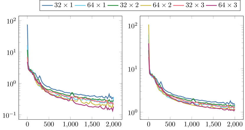
Figure 1: Average training (left) and validation (right) loss of different GRU-cells per patch (smoothed with gnuplots smooth bezier curve): A cell with dimension $m\times n$ consists of $n$ GRUs stacked on top of each other, where the hidden states $h$ are of size $m$.

GRU dims	#parameters		time
$32\times 1$	8544	$($1.00$)$	$7039\text{\,}\mathrm{s}$	$($1.00$)$
$64\times 1$	23232	$($2.72$)$	$7238\text{\,}\mathrm{s}$	$($1.02$)$
$32\times 2$	14688	$($1.72$)$	$8055\text{\,}\mathrm{s}$	$($1.14$)$
$64\times 2$	47808	$($5.60$)$	$8335\text{\,}\mathrm{s}$	$($1.18$)$
$32\times 3$	20832	$($2.44$)$	$9158\text{\,}\mathrm{s}$	$($1.30$)$
$64\times 3$	72384	$($8.47$)$	$9573\text{\,}\mathrm{s}$	$($1.36$)$

Table 1: GRU dimensions, parameters and the training time. In parentheses we list the factor compared to GRU $32\times 1$.

3.3 Application performance

Once trained, the network is used in the DNN-MG solver described in Section 2. Table 2 collects the runtimes for the overall simulation over 1050 time steps as well as the time required for evaluating the neural network in DNN-MG. In most cases, the neural network contributes less than 4% to the overall computational time. We further note that about $1.5\text{\,}\mathrm{s}$ of the network evaluation time must be attributed to data processing and communication between the finite element library and PyTorch. In an optimized implementation this time could most likely be reduced substantially.

The observed scaling in Tab. 2 does not always agree with what one would expect from the neural networks sizes in Tab. 1. There are multiple reasons for this. First, when the neural network correction is highly inaccurate then we need more Newton iterations in the next time step, resulting in higher runtimes such as for the $32\times 1$ network. High quality predictions, on the other hand, improve the runtimes and for the $64\times 3$ GRU-cell, for example, the time associated with the assembly routines was reduced by a factor of 4. Second, if the network deteriorates the solution and convergence of the Newton iteration is too slow we switch off the prediction for this time step. If this happens often, it leads to significantly less network evaluations and thus reduces runtimes of the network (this causes the spikes e.g. for $64\times 1$, $64\times 2$) although at the price of a loss in accuracy.

In summary, the networks take up only a small fraction of the runtime and may even reduce the overall runtime through faster convergence of the Newton iteration. For the largest network $64\times 3$, for example, we achieve a speedup of almost 100% compared to the solution without a network. However, an ill-suited network can also negatively affect the convergence and hence slow down computations.

type	runtime	NN-Eval
MG($L+1$)	$538.45\text{\,}\mathrm{s}$		$($0$\%)$
MG($L$)	$453.06\text{\,}\mathrm{s}$		$($0$\%)$
$32\times 1$	$705.53\text{\,}\mathrm{s}$	$21.84\text{\,}\mathrm{s}$	$($3.1$\%)$
$64\times 1$	$284.63\text{\,}\mathrm{s}$	$2.85\text{\,}\mathrm{s}$	$($1.0$\%)$
$32\times 2$	$257.72\text{\,}\mathrm{s}$	$7.44\text{\,}\mathrm{s}$	$($2.9$\%)$
$64\times 2$	$224.95\text{\,}\mathrm{s}$	$4.14\text{\,}\mathrm{s}$	$($1.8$\%)$
$32\times 3$	$200.42\text{\,}\mathrm{s}$	$11.01\text{\,}\mathrm{s}$	$($5.5$\%)$
$64\times 3$	$230.6\text{\,}\mathrm{s}$	$5.47\text{\,}\mathrm{s}$	$($2.3$\%)$

Table 2: Timing results for the simulations with the different GRUs we tested with runtime referring to the timing of the whole simulation and NN-eval the time spent on evaluating the neural network. In general $\approx$1.5\text{\,}\mathrm{s}$$ of the latter is spent on data processing. In parentheses we specify the time taken relative to the runtime in percent.

3.4 Accuracy of the networks

To compare the approximation power of the different neural network configurations, we evaluate the solution to the benchmark problem with respect to three functionals and also compute the error in the computed velocities and pressures.

The first functional we consider is the squared divergence

$$J_{\text{div}}(v(t))=\int_{\Omega}|\nabla\cdot v(t)|^{2}\,\text{d}x.$$

We know that the exact solution should satisfy $J_{\text{div}}(v)=0$. However, since our finite element approach is not strictly divergence free and since we are adding artificial stabilization terms, compare (4), the numerical solution will carry a divergence error that is also present in the training data. Hence, also the neural network correction will not be exactly divergence free although it should not deteriorate it further.

As suggested in [21], the second and third functional we are considering are the drag and lift forces acting on the obstacle

$$J_{\text{drag}}(v(t),p(t)) =-\int_{\partial\Gamma}\big{(}\frac{1}{Re}\nabla v(t)-p(t)I\big{)}\vec{n}\cdot\vec{e}_{x}\,\text{d}s,$$

$$J_{\text{lift}}(v(t),p(t)) =-\int_{\partial\Gamma}\big{(}\frac{1}{Re}\nabla v(t)-p(t)I\big{)}\vec{n}\cdot\vec{e}_{y}\,\text{d}s,$$

where we denote by $\Gamma$ the boundary of the obstacle, by $\vec{n}$ the unit normal vector pointing into the obstacle and by $\vec{e}_{x},\vec{e}_{y}$ the Cartesian unit vectors.

Figure 2: Divergence $J_{\text{div}}(v(t))$, drag $J_{\text{drag}}(v(t),p(t))$, lift $J_{\text{lift}}(v(t),p(t))$ (from left to right) for the coarse multigrid solution MG($L$), a high fidelity finite element reference solution MG($L+1$) and DNN-MG solutions for different GRU configurations.

Figure 2 shows all three functionals over the temporal interval $[9\,\mathrm{s},10\,\mathrm{s}]$, where the solution reached the periodic limit cycle (the phase were adjusted so that they agree on the first maximum in $[9\,\mathrm{s},10\,\mathrm{s}]$). We use a high resolution simulation MG($L+1$) as reference and MG($L$), that is the uncorrected simulation on level $L$, as base line. We observe that most functional outputs are significantly improved by DNN-MG with the best performing neural networks. Nearly exact values are obtained in case of the lift functional (right) but also drag (middle) is getting close to the reference value, in particular for $64\times 3$. For the divergence $J_{\text{div}}$ the improvement is more modest although compared to our previous results  [15] ([14, Fig. 1] in the corresponding preprint) with a network with $32\times 1$ GRU cells we still obtain a lower divergence.

In Fig. 3 we show the relative $l_{2}$ errors of the velocity and pressure with respect to the fine mesh solution MG($L+1$). The results demonstrate that the largest network $64\times 3$ is able to produce robust and accurate predictions for large time intervals. This network is also able to substantially reduce the phase error that results from the interplay between spatial and temporal discretization [20, 7] and leads to lower frequency oscillations on coarser meshes. Our previous results and the smaller networks show the same effect for the DNN-MG approach (low frequency oscillations in Fig. 3) but using a larger neural network cures this defect. We also refer to Fig. 2 which shows (e.g. in the case of the lift functional) that the GRU $64\times 3$ solution is almost perfectly in phase with the fine mesh solution MG($L+1$) while a lower frequency is found for the coarse mesh MG($L$).

4 Discussion

The presented results show the scalability of the DNN-MG method with respect to the network size. We observed that larger networks lead to DNN-MG simulations that capture flow behavior more accurately. At the same time, the increased number of parameters in the network has little impact on the training times and can (through the faster convergence of the Newton solve) even improve the runtime performance compared to a standard MG solver. Smaller networks are often not able to capture the flow behavior and even render the solution useless at times. In some cases they also have a negative impact on the runtime performance due to the interaction of the neural network and the Newton solve.

Figure 3: Relative errors for velocity (left) and pressure (right) compared to the reference solution on level $L+1$ for the coarse solution on level $L$ and DNN-MG with different neural network configurations.

5 Conclusion

We have investigated the scalability of the DNN-MG method with respect to the neural network size in terms of accuracy, runtime, and training time. We showed that larger networks are able to more accurately predict flow features and this allowed us to substantially improve over previous results for the DNN-MG method. In particular, our largest network $64\times 3$ is able to recover the flow frequency of the high fidelity simulations and through this we obtained velocity and pressure errors not attainable before. The divergence is now also at least as good as for the standard multigrid simulation without any additional effort, cf. [14]. Importantly, the improved accuracy comes at virtually no additional cost in terms of runtime and are now able to improve over a standard multigrid simulation by almost 100%.

The presented results lead to further research directions we would like to investigate in the future. One question is when the network size saturates and how the required amount of training data scales with the number of network parameters. The presented results in 2D provide also a promising basis for a hybrid finite element / neural network simulation for the Navier-Stokes equations in 3D which we would like to consider in the future. Finally, our practical findings provide a strong motivation to address more theoretical questions such as the stability, consistency and convergence of DNN-MG.

Acknowledgement

NM acknowledges support by the Helmholtz-Gesellschaft grant number HIDSS-0002 DASHH.

References

- [1] R. Becker and M. Braack “A Finite Element Pressure Gradient Stabilization for the Stokes Equations Based on Local Projections” In Calcolo 38.4, 2001, pp. 173–199
- [2] R. Becker et al. “The Finite Element Toolkit Gascoigne 3d”
- [3] M. Braack and P.. Mucha “Directional Do-Nothing Condition for the Navier-Stokes Equations” In J. Comp. Math. 32.5, 2014, pp. 507–521
- [4] B. Chang et al. “Reversible Architectures for Arbitrarily Deep Residual Neural Networks” In AAAI Conference on Artificial Intelligence, 2018
- [5] W. E “A Proposal on Machine Learning via Dynamical Systems” In Communications in Mathematics and Statistics 5.1, 2017, pp. 1–11 DOI: 10.1007/s40304-017-0103-z
- [6] E. Haber and L. Ruthotto “Stable architectures for deep neural networks” In Inverse Problems 34.1 IOP Publishing, 2017, pp. 014004 DOI: 10.1088/1361-6420/aa9a90
- [7] D. Hartmann, C. Lessig, N. Margenberg and T. Richter “A Neural Network Multigrid Solver for the Navier-Stokes Equations” In submitted, 2020 arXiv:2008.11520
- [8] J.. Heywood, R. Rannacher and S. Turek “Artificial Boundaries and Flux and Pressure Conditions for the Incompressible Navier-Stokes Equations” In Int. J. Numer. Math. Fluids. 22, 1992, pp. 325–352
- [9] M.. Kasim et al. “Up to two billion times acceleration of scientific simulations with deep neural architecture search”, 2020 arXiv: http://arxiv.org/abs/2001.08055
- [10] Y. LeCun, Y. Bengio and G. Hinton “Deep learning” In Nature 521.7553 Nature Publishing Group, 2015, pp. 436–444 DOI: 10.1038/nature14539
- [11] Z. Li et al. “Fourier Neural Operator for Parametric Partial Differential Equations”, 2020 arXiv:2010.08895 [cs.LG]
- [12] Z. Li et al. “Neural Operator: Graph Kernel Network for Partial Differential Equations”, 2020 arXiv:2003.03485 [cs.LG]
- [13] L. Lu, P. Jin and G.. Karniadakis “DeepONet: Learning nonlinear operators for identifying differential equations based on the universal approximation theorem of operators”, 2020 arXiv:1910.03193 [cs.LG]
- [14] Nils Margenberg, Christian Lessig and Thomas Richter “Structure Preservation for the Deep Neural Network Multigrid Solver”, 2020 arXiv: http://arxiv.org/abs/2012.05290
- [15] Nils Margenberg, Christian Lessig and Thomas Richter “Structure Preservation for the Deep Neural Network Multigrid Solver” accepted In Electronic Transactions on Numerical Analysis, 2021
- [16] Adam Paszke et al. “Automatic Differentiation in PyTorch” In NIPS Autodiff Workshop, 2017
- [17] M. Raissi and G.. Karniadakis “Hidden physics models: Machine learning of nonlinear partial differential equations” In Journal of Computational Physics 357 Academic Press, 2018, pp. 125–141 DOI: 10.1016/J.JCP.2017.11.039
- [18] M. Raissi, P. Perdikaris and G.E. Karniadakis “Physics-informed neural networks: A deep learning framework for solving forward and inverse problems involving nonlinear partial differential equations” In Journal of Computational Physics 378, 2019, pp. 686–707 DOI: https://doi.org/10.1016/j.jcp.2018.10.045
- [19] T. Richter “Fluid-Structure Interactions. Models, Analysis and Finite Elements” 118, Lecture Notes in Computational Science and Engineering Springer, 2017
- [20] Thomas Richter and Nils Margenberg “Parallel Time-Stepping for Fluid-Structure Interactions” In Mathematical Modelling of Natural Phenomena, 2021 DOI: 10.1051/mmnp/2021005
- [21] M. Schäfer and S. Turek “Benchmark computations of laminar flow around a cylinder. (With support by F. Durst, E. Krause and R. Rannacher)” In Flow Simulation with High-Performance Computers II. DFG priority research program results 1993-1995, Notes Numer. Fluid Mech. 52 Vieweg, Wiesbaden, 1996, pp. 547–566