Unpredictability and entanglement in open quantum systems

Abstract

We investigate dynamical many-body systems capable of universal computation, which leads to their properties being unpredictable unless the dynamics is simulated from the beginning to the end. Unpredictable behavior can be quantitatively assessed in terms of a data compression of the states occurring during the time evolution, which is closely related to their Kolmogorov complexity. We analyze a master equation embedding of classical cellular automata and demonstrate the existence of a phase transition between predictable and unpredictable behavior as a function of the random noise introduced by the embedding. We then turn to have this dynamics competing with a second process inducing quantum fluctuations and dissipatively driving the system to a highly entangled steady state. Strikingly, for intermediate strength of the quantum fluctuations, we find that both unpredictability and quantum entanglement can coexist even in the long time limit. Finally, we show that the required many-body interactions for the cellular automaton embedding can be efficiently realized within a variational quantum simulator platform based on ultracold Rydberg atoms with high fidelity.

I Introduction

The discovery of problems that are fundamentally undecidable is one of the most striking results in the history of mathematics Gödel (1931); Turing (1937). For physical systems, this means that certain problems such as the existence of a spectral gap in a many-body system can be undecidable as well Lloyd (1993); Cubitt et al. (2015). Likewise, the long-term dynamics of a physical system can be unpredictable in the sense that the only way to compute observables is to simulate the system from the beginning to the end Wolfram (1984a). Here, we show that driven-dissipative quantum systems provide an ideal platform to study such fascinating systems and to explore the hitherto largely unknown relation of this unpredictably with entanglement that is absent in classical dynamical systems. Strikingly, while we find that the statistical aspects of entangled states inherently drive the system towards chaotic behavior, we find that under the right conditions, unpredictability and entanglement can coexist in the steady state.

The dynamical behavior of unpredictable systems is most readily analyzed in the framework of cellular automata, as one can show rigorously that these systems are Turing-complete and hence unpredictable Margolus (1984); Berlekamp et al. (2004); Cook (2004); Neary and Woods (2006). However, common quantum version of cellular automata Brennen and Williams (2003); Raussendorf (2005); Arrighi et al. (2008); Bleh et al. (2012); Hillberry et al. (2021) rely on purely unitary dynamics and are therefore challenging to realize without having access to fault-tolerant quantum computers. For this reason, variants of quantum cellular automata using open quantum many-body systems Lesanovsky et al. (2019); Wintermantel et al. (2020) appear to be a much more promising route to investigate the interplay between unpredictability and inherently quantum properties of the dynamics like quantum superpositions and entanglement.

In this article, we provide an embedding of cellular automata (CA) into a Lindblad master equation, which is commonly used within open quantum systems. To this end, we consider two coupled one-dimensional (1D) chains representing the state of the automaton at the time step $t$ and $t+1$, respectively, see Fig. 1a. Here, we focus on a class of elementary cellular automata introduced by Wolfram Wolfram (1983), as this class contains Turing-complete automata and can be realized in the embedding using at most four-body interactions. The mapping of CAs onto master equation requires a periodic switching of the chains, with the exact CA dynamics being recovered in the limit of infinite cycle times. Interestingly, the imperfections to the perfect CA rules introduced by finite cycle times do not immediately destroy unpredictability, as shown using an information-theoretical complexity measure based on data compression of the states during the dynamical evolution of the system Zenil (2010). We then introduce quantum fluctuations by adding a second set of terms to the master equation that drive the system to a highly-entangled Rokhsar-Kivelson state Roghani and Weimer (2018). We explore the interplay between unpredictability and entanglement by modifying the relative rates of the two competing dynamics, finding an intermediate regime in which both entanglement and unpredictability coexist. Finally, we demonstrate the experimental feasibility of our approach by investigating a platform based on ultracold Rydberg atoms Browaeys and Lahaye (2019); Morgado and Whitlock (2021). To this end, we introduce an open system version of a variational quantum estimation algorithm Peruzzo et al. (2014); Moll et al. (2018); Kokail et al. (2019) and show that the full dynamics including dissipative many-body interactions can be realized efficiently.

	a
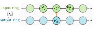
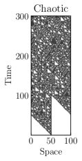
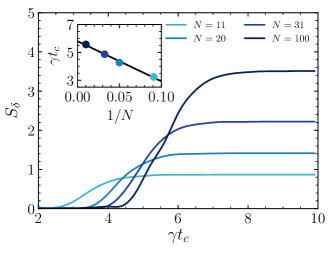
b	c	d

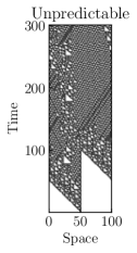
Figure 1: (a) Physical implementation of elementary CA on two rings of lattice sites, with the input and output ring switching after a cycle time $t_{c}$. (b) Typical trajectory of the rule 110 CA evolving from a single cell in the 1 state (black) for a short cycle time $t_{c}=4/\gamma$, leading to Class III chaotic behavior. (c) Increasing the cycle time induces a transition to unpredictable behavior as shown by the slope $S_{\delta}$ of the characteristic compression exponent. Finite size scaling (inset) points to a value of $\gamma t_{c}=5.80\pm 0.08$ for the transition in the thermodynamic limit. (d) Typical trajectory in the unpredictable Class IV phase at a large cycle time $t_{c}=10/\gamma$. At longer times, emergent glider structures propagating through the systems become clearly visible. Calculations were made at $n=50$ and $t=300$ to obtain convergence in $S_{\delta}$. For each initial state, 100 Monte-Carlo samples were taken.

II Complexity classes and unpredictability

The fundamental properties of the dynamical evolution of translation invariant dynamical systems like CAs can be broadly captured in four distinct classes Wolfram (1984a); Martinez et al. (2013), referring to their generic behavior for almost all initial states. Class I refers to a fast evolution towards a steady state. Class II systems evolve towards periodic limit-cycle oscillations. Class III systems are chaotic, which can be captured in terms of a positive Lyapunov exponent Eckmann and Ruelle (1985) and fast relaxation of entropic measures to a constant value that is large. Finally, Class IV systems exhibit diverging transient times and are exhibiting emerging structures that can be very complex. It is conjectured that Class IV systems are capable of universal computation and hence their behavior in the thermodynamical limit are fundamentally uncomputable Wolfram (1984a). It has also been discussed that Class IV systems are critical phases at the edge between regular periodic and chaotic behavior Langton (1990).

While chaotic (i.e., Class III) systems are sometimes also classified as unpredictable because of their sensitvity to changes in the initial condition, the notion of unpredictability we employ here is more strict, as statements about some long-time properties of chaotic systems are possible in terms of statistical averages, e.g., by coarse-graining the system under consideration Cotler et al. (2017). Our notion of unpredictability is closely connected to the concept of sophistication in computer science Koppel (1987), which can also be understood as capturing the complexity of systems at a coarse-grained level Aaronson et al. (2014).

The quantitative identification of Class IV behavior is extremely challenging, requiring the computation of observables that go beyond entropic measures or Lyapunov exponents geared to the analysis of Class III systems. For systems of discrete variables, one possibility is an information-theoretical analysis of the computational strings encoding the state of the system. For each string $S$, the algorithmic complexity is given by its Kolmogorov complexity $\mathcal{K}(S)$, which is defined as the length of the shortest program that can output $S$ Li and Vitányi (2008). However, Kolmogorov complexity itself is an uncomputable quantity, preventing a direct practical application. Fortunately, it is possible to construct practically useful upper bounds to the Kolmogorov complexity by considering the compression length $\mathcal{C}(S)$ satisfying

$$\mathcal{C}(S)=\mathcal{C}_{c}(S)+\mathcal{C}_{0}\geq\mathcal{K}(S),$$ (1)

where $\mathcal{C}_{c}(S)$ is the compressed length of $S$ using a compression program of length $\mathcal{C}_{0}$, the latter being the same for all strings $S$.

For the classification of dynamical systems, the Kolmogorov complexity (or the compression length is not sufficient to capture unpredictability, as the (pseudo-)randomness inherent in chaotic systems will generically lead to large values of $\mathcal{K}(S)$ even for Class III systems. However, it is possible to differentiate Class III and Class IV by looking at the compression length for different initial states Zenil (2010); Martinez et al. (2013). For chaotic Class III systems, the Kolmogorov complexity does not depend on the particular initial state, i.e., differential measures of Kolmogorov complexity are vanishing. Importantly, this is not the case in Class IV systems, where the Kolmogorov complexity strongly depends on the initial state. This can be understood as the initial state encoding a program that is run using the universal computing capabilities of the Class IV system. Some programs can produce simple computing results exhibiting a low Kolmogorov complexity, while others can lead to arbitrary complex computations. This can be captured quantitatively in the form of a characteristic compression exponent Zenil (2010), which is a generalization of the Lyapunov exponent to algorithmic complexity. It is given by

$$\delta_{n}(t)=\sum_{j=1}^{n-1}\frac{\big{|}\mathcal{C}_{c}(S_{j}(t))-\mathcal{C}_{c}(S_{j+1}(t))\big{|}}{n-1},$$ (2)

where $S_{j}(t)$ refers to the string representation of the state at time $t$ for the $j$th initial state and the sum runs over $n$ initial states in total. For systems with binary degrees of freedom, this can be achieved by using the Gray code Gray (1953), which ensures that the changes observed in the compression lengths are not stemming from discontinuities within the initial conditions Zenil (2010). For the compression algorithm, we use the zlib.compress function provided by Python 3.6.9., which provides a widely used implementation of the DEFLATE algorithm Deutsch (1996).

Generically, $\delta_{n}(t)$ will increase linearly with time in the long time limit. Therefore, the slope $S_{\delta}=d\delta_{n}(t)/dt$ of the characteristic exponent for sufficiently large $n$ is the actual quantity that can be used to identify Class IV systems.

III Embedding of elementary cellular automata

Elementary cellular automata (ECAs) Wolfram (1984b) are two-level systems on a 1D lattice, where the state $i$ at the dimensionless time $t+1$ depends only on the states of the sites $i-1$, $i$, and $i+1$ and time $t$. In total, there are $2^{2^{3}}=256$ different possible ECA rules, which can be enumerated according to the binary representation of their ruleset. Here, we will be interested in rule 110 (or its binary complement 137), see Tab. 1 for the ruleset, as this ECA has been proven to be capable of universal computation Cook (2004) and hence belongs into Class IV.

State at $t$	111	110	101	100	011	010	001	000
Central site at $t+1$	0	1	1	0	1	1	1	0

Table 1: Ruleset for ECA rule $110=01101110_{2}$ indicating how the central site is updated. The ruleset for the corresponding rule 137 can be found by inverting all inputs and outputs.

Most ECA rules are irreversible, as each output bit depends on three input bits. This prevents an implementation in a quantum system in terms of unitary operations and instead requires the use of a dissipative quantum channel $\mathcal{V}$ providing the mapping $\rho(t+1)=\mathcal{V}\rho(t)$ for the quantum state $\rho$. The generator of such a quantum channel can be expressed in terms of a purely dissipative quantum master equation in Lindblad form,

$$\frac{d}{dt}\rho=\gamma\sum\limits_{i}\left(c_{i}\rho c_{i}^{\dagger}-\frac{1}{2}\left\{c_{i}^{\dagger}c_{i},\rho\right\}\right),$$ (3)

with $c_{i}$ being the associated quantum jump operators Breuer and Petruccione (2002) and $\gamma$ being the characteristic rate of the dynamics. Note that the channel $\mathcal{V}$ is only implemented in the steady state, i.e., in the infinite time limit. For the case of a finite evolution time $t_{c}$, this means that the evolution of the corresponding cellular automaton becomes probabilistic. However, since a finite error rate can be recovered in classical systems by error correction codes, one can expect that Class IV systems capable of universal computation can tolerate a finite amount of computational errors introduced by the probabilistic update scheme. Interestingly, this setting allows to treat the cycle time $t_{c}$ as a control parameter, which allows to alter the dynamical properties of the system under consideration in a relatively simple way.

For practical implementation purposes, it is highly desirable that the quantum jump operators are quasi-local, i.e., they act only on a small subset of the total Hilbert space. Within the ECA framework, this can be readily achieved by considering a second copy of the system, in which the state at time $t+1$ is prepared, see Fig. 1a. After a time $t_{c}$, the role of the two copies is reversed and the second copy is taken as the input for the creation of the new state at time $t+2$ in the first copy.

IV Cycle time phase transition

IV.1 Purely classical dynamics

Let us now turn to investigating how the dynamics of the rule 110 CA change with the cycle time $t_{c}$. Since the dynamics is purely classical, the master equation can be simulated efficiently using Monte-Carlo sampling. Fig. 1c shows that the slope of the characteristic compression exponent $S_{\delta}$ indeed undergoes a phase transition from a chaotic Class III phase (Fig. 1b) with vanishing $S_{\delta}$ to an unpredictable Class IV phase (Fig. 1d) with finite $S_{\delta}$. We also observe that the value of $S_{\delta}$ significantly depends on the system size $N$, which can be attributed to the appearance of emergent glider structures much larger than the three-site unit cell of the CA Cook (2004). For example, the smallest system size in which all types of gliders can be realized is $N=11$. Nevertheless, we can still perform finite size scaling of $S_{\delta}$ by considering only those system sizes at which $S_{\delta}$ is at a local maximum, a technique that has been used previously in the analysis of systems with strong incommensurability effects Weimer and Büchler (2010); Arora et al. (2015). Here, we find the phase transition to occur at $t_{c}=5.80\pm 0.08$ in the thermodynamic limit. Note that it might seem surprising that we are able to perform finite size scaling in a system with unpredictable behavior, as unpredictability is directly tied to a breakdown of finite size scaling theory Cubitt et al. (2015). However, here one of the two phases has the computable value of zero for $S_{\delta}$ in the thermodynamic limit, which means that the phase transition can successfully detected by observing deviations from $S_{\delta}$ vanishing for increasing system sizes.

IV.2 Competition with entanglement

So far, we have not addressed including quantum fluctuations into the dynamics. While there are many different proposals for CA dynamics within quantum systems Brennen and Williams (2003); Bleh et al. (2012); Lesanovsky et al. (2019); Wintermantel et al. (2020); Klobas and Prosen (2020); Wilkinson et al. (2020), here we focus on the case where we have two competing dynamics $\mathcal{L}_{c}$ and $\mathcal{L}_{q}$, which are both generators satisfying the purely dissipative Lindblad form of Eq. (3), i.e., the full Lindblad generator $\mathcal{L}$ is given by

$$\mathcal{L}=\sin^{2}\left(\phi\frac{\pi}{2}\right)\mathcal{L}_{c}+\cos^{2}\left(\phi\frac{\pi}{2}\right)\mathcal{L}_{q},$$ (4)

where $\phi$ is a parameter that interpolates between the fully quantum and fully classical dynamics. This approach has the advantage that the relevant observable $S_{\delta}$ for detecting unpredictability can be carried over to the quantum case by identifying the $i$th bit in the string $S_{j}$ by the most likely measurement result when sampled over many trajectories.

In the following, we will be interested in the case where the quantum part of the dynamics is carefully chosen to have its unique steady state being highly entangled. For this, we choose a recently introduced quantum master equation that prepares the system in a Rokhsar-Kivelson state Roghani and Weimer (2018), which is given by

$$|\psi_{RK}\rangle=\frac{1}{\sqrt{Z}}\prod_{k}^{N}(1-P_{k-1}\sigma_{+}^{k}P_{k+1})|00\cdots 0\rangle,$$ (5)

where $P_{k}=\mathopen{|}0\mathclose{\rangle}\mathopen{\langle}0\mathclose{|}_{k}$ and $Z$ is a normalization constant. This state is an equal-weight superposition of all states that have no adjacent qubits in the $\mathopen{|}1\mathclose{\rangle}$ state. The jump operators $c_{i}^{q}$ required to prepare $\mathopen{|}\psi_{RK}\mathclose{\rangle}$ can be brought into a similar form as the one for the rule 110, i.e.,

$$c_{i}^{q}=\sum\limits_{k}O_{\bar{i},k}Q_{i,k}$$ (6)

where $O_{\bar{i},k}$ is an operator acting on the sites $i-1$, $i$, and $i+1$ on the output ring, while $Q_{i,k}=\mathopen{|}k\mathclose{\rangle}\mathopen{\langle}k\mathclose{|}$ is a projection operator acting on the corresponding sites of the input ring. The index $k$ runs over all eight basis states on the sites $i-1,$ $i$, and $i+1$. Table 2 shows a set of operators that lead to $\mathopen{|}\psi_{RK}\mathclose{\rangle}$ being the dark state of the dynamics, satisfying $c_{i}^{q}\mathopen{|}\psi_{RK}\mathclose{\rangle}=0$. To observe the interplay between unpredictability and entanglement, it is helpful to make the two competing dynamics closely aligned with each other. One can see that $\mathopen{|}\psi_{RK}\mathclose{\rangle}$ will have more 0s than 1s in its binary representation due to the action of the projection operators $P_{k}$. On the other hand, the dynamics of rule 110 is slightly biased towards the 1 state, as there are more 1s than 0s in the output set. Therefore, we consider the binary complement rule $137=10001001_{2}$, which is then also biased towards the 0 state, but having otherwise identical properties as rule 110.

State $k$ at $t$	111	110	101	100	011	010	001	000
Operation $O_{k}$	$\mu$	$\sigma_{-}$	$\mu$	$\mu$	$\mu$	$\mu$	$\mu$	$\mu$

Table 2: Ruleset to prepare the Rokhsar-Kivelson state $\mathopen{|}\psi_{RK}\mathclose{\rangle}$. The operator $\mu_{\bar{i}}=P_{\bar{i}-1}{\mathopen{|}-\mathclose{\rangle}\mathopen{\langle}+\mathclose{|}_{\bar{i}}}P_{\bar{i}+1}$ acts on the three sites surrounding $\bar{i}$ on the output ring, with $\mathopen{|}\pm\mathclose{\rangle}=(\mathopen{|}0\mathclose{\rangle}\pm\mathopen{|}1\mathclose{\rangle})$. The operator $\sigma_{-}$ acts only on the site $\bar{i}$.

To further align the two competing dynamics, we additionally split the dynamics into two parts, each being $t_{c}/2$ long. During the first part, both the classical part $\mathcal{L}_{c}$ and the quantum part $\mathcal{L}_{q}$ are active, while during the second part only the classical dynamics is acting on the system. All observables are evaluated at the time $t_{c}/2$.

a

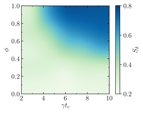
b

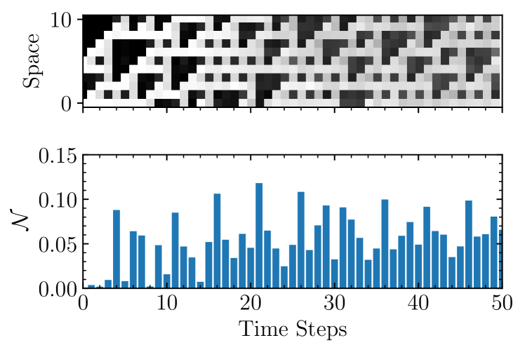
Figure 2: Competition between classical and quantum dynamics. (a) Slope $S_{\delta}$ of the characteristic compression exponent as a function of the cycle time $t_{c}$ and the interpolation parameter $\phi$, showing an extended region of unpredictable Class IV behavior even in the presence of quantum fluctuations. (b) Average over 50 Monte-Carlo samples of a single initial configuration for $\gamma t_{c}=10$ and $\phi=0.6$. Although quantum fluctuations lead to a washing out of the patterns, the emergent structures remain clearly visible. The negativity $\mathcal{N}$ rapidly increases and remains finite in the long time limit.

Let us now turn to a numerical investigation of the competition between the classical rule 137 dynamics $\mathcal{L}_{c}$ and the quantum dynamics $\mathcal{L}_{q}$ preparing the Rokhsar-Kivelson state. Figure 2 shows the unpredictability of the system in terms of the slope $S_{\delta}$ of the characteristic compression exponent as a function of the cycle time $t_{c}$ and the interpolation parameter $\phi$, as well as the entanglement of the system in terms of the negativity

$$\mathcal{N}(\rho)=\frac{\left\lVert\rho^{T_{A}}\right\rVert_{1}-1}{2},$$ (7)

where $\left\lVert.\right\rVert_{1}$ denotes the trace norm and $\rho^{T_{A}}$ is the partial transpose of $\rho$ with respect to the subsystem $A$ Vidal and Werner (2002). Calculations were performed using massively parallelized wave-function Monte-Carlo simulations Johansson et al. (2013) for 22 sites, improving the previously reported largest system size for simulations retaining the full Hilbert space Raghunandan et al. (2018). For the classical limit $\phi\to 1$, we recover the classical transition to an unpredictable Class IV phase reported in Sec. IV.1. However, this transition remains observable away from the classical limit as well. Crucially, we also find a nonzero negativity for sufficiently low values of $\phi$, meaning that unpredictability and entanglement can coexist in the system. Finally, when the interpolation parameter $\phi$ is decreased further, unpredictable Class IV behavior is destroyed by quantum fluctuations.

V Variational quantum simulation

The realization of the jump operators for the classical and quantum dynamics requires the implementation of four and six-body interactions, respectively. While such high-order interactions can be readily engineered in digital quantum simulators Weimer et al. (2010, 2011), recently developed techniques for the variational preparation of quantum states Peruzzo et al. (2014); Moll et al. (2018); Kokail et al. (2019) can be adapted for the quantum simulation of open system dynamics, especially on noisy intermediate-scale quantum devices. Basically, variational quantum simulation (VQS) is a hybrid classical-quantum approach that can approximately reproduce the dynamics of a quantum system without explicit realization of the corresponding Hamiltonian.

Within our VQS approach, we can realize the time evolution of largely arbitrary open quantum many-body systems according to a Lindblad quantum master equation. To this end, we consider the dynamics of an observable $O$ in the Heisenberg picture,

$$\frac{dO}{dt}\equiv\mathcal{L}_{H}O=i[H,O]+\sum\limits_{i}^{N}{L_{i}}^{\dagger}OL_{i}-\frac{1}{2}\big{\{}L_{i}^{\dagger}L_{i},O\big{\}}.$$ (8)

The strategy behind VQS is to consider a variational parametrization of the state $\rho(t+\tau)$ after a timestep $\tau$, given the state $\rho(t)$ at time $t$ and the dynamics according to the quantum master equation. Our approach is based on the variational principle for open quantum systems Weimer (2015), which also has been generalized towards variational approximation of the time evolution, both in the Schrödinger Overbeck and Weimer (2016) and in the Heisenberg picture Pistorius and Weimer (2020). Within the latter, one can introduce a variational cost functional $F_{v}$ given by

$$F_{v}=\sum_{i}\Big{|}\big{\langle}O_{i}(t+\tau)\big{\rangle}-\big{\langle}O_{i}(t)\big{\rangle}-\frac{\tau}{2}\mathcal{L}_{H}[O_{i}(t)+O_{i}(t+\tau)]\Big{|},$$ (9)

which realizes a discretized version of the master equation that is correct up to second order in $\tau$. Crucially, the sum does not need to run over a complete set of observables to achieve accurate results Pistorius and Weimer (2020).

Having defined the variational cost function, we also need to specify the parameterization of the density matrix $\rho$ using a set of variational parameters $\boldsymbol{\theta}$. For this, we consider a variational circuit consisting of three parts, see Fig. 3: (i) Coherent single qubit rotations, (ii) dissipative single qubit damping, and (iii) global unitary time evolution under an interacting many-body Hamiltonian that can be implemented efficiently.

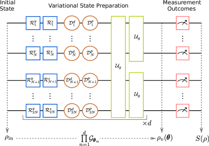
Figure 3: Sketch of the variational quantum simulation scheme. A quantum state $\rho_{v}(\boldsymbol{\theta})$ is generated from an initial state $\rho_{\text{in}}$ and a set of variational parameters $\boldsymbol{\theta}=\{\boldsymbol{\theta}_{n}\}_{n=1}^{d}$ for $d$ layers. The variational circuit consists of local Pauli rotations $\mathcal{R}(\boldsymbol{\theta}_{n})$, local dissipation operators $\mathcal{D}(\boldsymbol{\theta}_{n})$, and global unitary operations $\mathcal{U}_{g}(\boldsymbol{\theta}_{n})$.

To be specific, we envision the qubits stored in the hyperfine ground states of ultracold atoms trapped in an optical tweezer array Endres et al. (2016); Barredo et al. (2016). While the coherent single qubit rotations are following from standard Pauli rotations around two independent axes using microwave driving, the dissipative dynamics is governed by two separate quantum channels realized by dissipative optical pumping of the qubit states ($\mathcal{D}_{d}$) and phase fluctuations mediated by noisy laser driving ($\mathcal{D}_{p}$), respectively. In the operator sum representation Nielsen and Chuang (2000) the two channels can be written as

$$\mathcal{D}_{\mu}(\rho)=\frac{1}{N}\sum_{j=1}^{N}\Big{[}D_{\mu_{1}}^{(j)}\rho{D_{\mu_{1}}^{(j)}}^{\dagger}+D_{\mu_{2}}^{(j)}\rho{D_{\mu_{2}}^{(j)}}^{\dagger}\Big{]},$$ (10)

where $\mu\in\{d,p\}$ and

$$D_{d_{1}}= \sqrt{1-e^{-\theta_{d}}}\sigma_{-},$$ (11)

$$D_{d_{2}}= P_{0}+e^{-\theta_{d}/2}P_{1},$$ (12)

$$D_{p_{1},p_{2}}= \sqrt{\frac{e^{-\theta_{p}/2}}{2}}\pm\sqrt{\frac{(1-e^{-\theta_{p}})}{2}}\sigma_{z},$$ (13)

depending on the variational parameters $\theta_{d}$ and $\theta_{p}$. Finally, the global unitaries $\mathcal{U}_{g}$ are implemented based on coupling the $\mathopen{|}1\mathclose{\rangle}$ state to a strongly interacting Rydberg state in a Rydberg dressing configuration Glaetzle et al. (2015); Zeiher et al. (2016); Overbeck et al. (2017); Helmrich et al. (2018), giving rise to the effective Hamiltonian

$$H_{0}=\frac{\Omega}{2}\sum_{i}\sigma_{x}^{(i)}+\sum_{i<j}\frac{C_{6}}{{|\textbf{r}_{i}-\textbf{r}_{j}|}^{6}}P_{1}^{(i)}P_{1}^{(j)},$$ (14)

where $\Omega$ indicates the Rabi frequency of the driving field and $C_{6}$ denotes the effective van der Waals coefficient of the Rydberg-dressed state. The global unitaries act first on both of the rails at the same time and then subsequently on each rail independently. The times $t_{1}$ and $t_{2}$ of these steps provide two additional variational parameters.

a

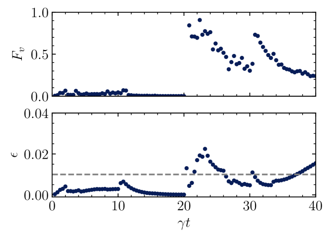
b

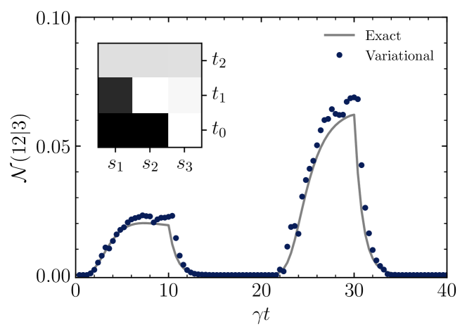
Figure 4: Benchmarking of the VQS approach for $\phi=0.5$ and $\gamma t_{c}=10$ for a system of $N=3$ sites, using $d=3$ variational layers. Variational norm $F_{v}$, error probability $\varepsilon$ (a) and quantum negativity $\mathcal{N}$ (b) as a function of time for the first two timesteps. The inset shows the density pattern in the output ring at the middle of the steps.

Let us now benchmark our VQS procedure for the quantum rule 137 dynamics using two rings of $N=3$ sites. In our simulations, we set $C_{6}/\Omega=100$ as this corresponds to a Rydberg blockade radius $r_{b}=\sqrt{6}{C_{6}/\Omega}\approx 2.15$ in units of the lattice spacing, which is comparable to the range of the multi-qubit jump operators in the quantum master equation. Furthermore, we choose a variational circuit depth of $d=3$. For the set of observables entering the variational cost function (9), we choose a complete set of 3-local Pauli operators per site, i.e., $4^{3}=64$ observables. Numerical optimization of the highly non-linear cost function is performed using a sequential quadratic programming algorithm Virtanen et al. (2020) in a layerwise fashion to avoid getting stuck in barren plateaus McClean et al. (2018).

Figure 4a shows variational norm $F_{v}$ and error probability $\varepsilon$ between the exact density matrix $\rho$ and variational state $\rho_{v}(\boldsymbol{\theta})$ at time $t$, defined in terms of the fidelity $F$ as

$$\varepsilon=1-F=1-\Bigg{[}\text{Tr}\sqrt{\sqrt{\rho_{v}(\boldsymbol{\theta})}\rho\sqrt{\rho_{v}(\boldsymbol{\theta})}}\Bigg{]}^{2}.$$ (15)

For $\phi=0.5$ and $\gamma t_{c}=10$, where unpredictability and quantum entanglement coexist, the results indicate overall errors less than $2\%$ for almost all data points. Figure 4b demonstrates that entanglement measured in terms of the negativity also shows good quantitative agreement with the exact dynamics, underlining the power of the VQS approach.

VI Conclusion

In summary, our work establishes a novel dynamical class of open quantum many-body systems that allow to study the interplay between computational properties and quantum effects. Strikingly, we have shown that computational unpredictability is not incompatible with quantum entanglement, but that the two can coexist with each other for a long time. Our results on the variational quantum simulation of these systems show that their experimental realization is possible using present technologies, making these systems also excellent candidates to observe a quantum advantage, given that their classical simulation is extremely challenging Weimer et al. (2021). In the future, it will be interesting to develop quantum analogs of the data compression approach for Class IV systems, using quantum compression algorithms Schumacher (1995); Jozsa et al. (1998); Rozema et al. (2014); Romero et al. (2017).