Non-Lorentzian Chaos and Cosmological Holography

Abstract

We study chaos in non-Lorentzian field theories, specifically Galilean and Carrollian conformal field theories in two dimensions. In a large central charge limit, we find that the Lyapunov exponent saturates the bound on chaos, conjectured originally for relativistic field theories. We recover the same Lyapunov exponent holographically by a shock-wave calculation in three-dimensional flat space cosmologies, providing further evidence for flat space holography.

Introduction. As aptly put by Edward Lorenz, a dynamical system becomes chaotic when the present determines the future, but the approximate present does not. In other words, the dynamics of the system is strongly sensitive to initial conditions. Colloquially, this is often described by flapping butterfly wings in Brazil, causing a tornado in Texas [1]. In this work, we discuss aspects of chaos in unconventional quantum field theories (QFTs) and their holographic manifestation in cosmological spacetimes.

The QFTs we consider are non-Lorentzian conformal field theories (CFTs) in two dimensions (2d). We begin our analysis with Galilean CFTs (GCFTs) [2], where the speed of light goes to infinity [3]. GCFTs are natural analogues of relativistic CFTs [4]. They are expected to arise as fixed points in renormalization group flows in the parameter space of Galilean QFTs. GCFTs appear in the non-relativistic limit of all known relativistic conformally invariant QFTs, e.g. massless scalars and fermions in all dimensions, sourceless electrodynamics, and pure non-Abelian gauge theories in four dimensions [5]. GCFTs are governed by the Galilean conformal algebra (GCA), which in 2d reads [6]

$$[L_{n},L_{m}] =(n-m)L_{n+m}+\frac{c_{L}}{12}\big{(}n^{3}-n\big{)}\delta_{n+m,0}$$ (1a)

$$[L_{n},M_{m}] =(n-m)M_{n+m}+\frac{c_{M}}{12}\big{(}n^{3}-n\big{)}\delta_{n+m,0}$$ (1b)

$$[M_{n},M_{m}] =0\qquad\qquad\qquad\qquad\qquad\quad n,m\in\mathbb{Z}\,.$$ (1c)

The $c$-numbers $c_{L}$ and $c_{M}$ are the central charges. We focus on the case $c_{L}=0$ and large $c_{M}$, since this will be most relevant for holographic applications of our results. With methods mirroring recent advances in relativistic 2d CFTs [7, 8, 9] we compute the diagnostics of chaos in GCFTs, specifically, the Lyapunov exponent, which characterizes the divergence of nearby trajectories in phase space.

We are also interested in another class of non-Lorentzian CFTs, viz. Carrollian CFTs (CCFTs). In Carrollian theories, the speed of light goes to zero, the opposite of the Galilean limit [3, 10, 11, 12]. Carrollian QFTs encompass any QFT defined on a null manifold [13]. Interestingly, in $d=2$, the Galilean and Carrollian groups are isomorphic. This isomorphism extends to their conformal versions [14]. Thus, 2d CCFTs are also governed by the algebra (1). Hence our answers, constructed for 2d GCFTs, are also valid for 2d CCFTs, albeit with an interchange of the spatial and temporal directions, and correspondingly different physical interpretations.

Finally, we use the holographic correspondence between 3d flat space and 2d CCFTs [14, 10] (elaborated on later) to holographically reproduce our field theory answers. Thermal states in the CCFT are dual to cosmological solutions called ‘Flat Space Cosmologies’ (FSC) [15, 16]. A calculation similar in spirit to the corresponding anti-de Sitter (AdS) black hole calculation with a shock-wave [17, 18] recovers the Lyapunov exponent that we find on the field theory side, giving further support to the proposed holographic correspondence in flat space. The main result of the present work is that both on the field theory and the gravity sides the Lyapunov exponent

$$\lambda_{L}=\frac{2\pi}{\beta}$$ (2)

saturates the conjectured bound on chaos [19] ($\beta$ is the inverse temperature).

Galilean CFT basics. We begin with some representation theory aspects of 2d GCFTs. The states of the theory are labeled by [6]

$$L_{0}|\Phi\rangle=\Delta_{\Phi}|\Phi\rangle\,,\qquad M_{0}|\Phi\rangle=\xi_{\Phi}|\Phi\rangle\,.$$ (3)

The action of $L_{n},M_{n}$ for $n>0$ on a state $|\Phi\rangle$ lowers the weight $\Delta_{\Phi}$. Hence in analogy with 2d CFTs, there is a notion of primary states $|\Phi\rangle_{p}$ satisfying

$$L_{n}|\Phi\rangle_{p}=M_{n}|\Phi\rangle_{p}=0,\qquad\forall n>0\,.$$ (4)

The rest of the module is built by acting with raising operators $L_{-n},M_{-n}$ for $n>0$ on a given primary state. Like in relativistic CFTs, there is also a state-operator correspondence $\Phi(0,\,0)\leftrightarrow|\Phi\rangle$. Below we exclusively use operators.

Chaos in classical systems can be diagnosed via the sensitivity to initial conditions using the Poisson bracket $\{x(t),p(0)\}=\frac{\partial x(t)}{\partial x(0)}$, which can grow as a sum of exponentials in $t$. The exponents therein are called Lyapunov exponents. The analogous quantity for a quantum system in a state that is described by a density matrix $\rho$ is $-\textnormal{Tr}(\rho[x(t),p(0)])$ [20]. Random phase cancellations that thermalize this quantity too soon are avoided by considering the square of the commutator. To study chaos of a thermal system in equilibrium at inverse temperature $\beta$ we thus consider the quantity [18, 21, 22, 23]

$$C(t)=-\langle[W(t),V(0)]^{2}\rangle_{\beta}\,,$$ (5)

which can be written in terms of time-ordered and out-of-time-ordered correlation functions (OTOCs). In a generic quantum many-body system the former approach a constant after the relaxation time $\beta$ while the OTOCs in contrast start at a large value and decrease over time, resulting in an increase of $C(t)$. Thus, one can use OTOCs to diagnose chaos [24]. To find chaotic behavior in a generic 2d GCFT we study the late time behavior of the following OTOC of pairs of local primary operators in a thermal state

$$\frac{\langle V^{\dagger}(0)W^{\dagger}(t)V(0)W(t)\rangle_{\beta}}{\langle V^{\dagger}(0)V(0)\rangle_{\beta}\langle W^{\dagger}(t)W(t)\rangle_{\beta}}\,,$$ (6)

and look for exponential decay of this OTOC. It is evaluated by mapping the 2d GCFT from the plane to a cylinder of radius $\beta$. We work in the approximation $c_{M}/\xi_{n}\gg 1$ , where $\xi_{n}=\xi_{V},\xi_{W}$ are the weights defined in (3). This allows the use of closed-form expressions of Galilean conformal blocks [26, 27, 28, 29, 30].

Chaotic correlators in GCFT. We start with a 2d GCFT on a complex plane with coordinates $(u,v)$. Consider two local scalar primary operators $V$ and $W$ with weights $(\Delta_{V},\xi_{V})$ and $(\Delta_{W},\xi_{W})$, respectively. Symmetry restricts the vacuum 4-point function [6]

$$\frac{\langle V^{\dagger}(u_{1},v_{1})V(u_{2},v_{2})W^{\dagger}(u_{3},v_{3})W(u_{4},v_{4})\rangle}{\langle V^{\dagger}(u_{1},v_{1})V(u_{2},v_{2})\rangle\langle W^{\dagger}(u_{3},v_{3})W(u_{4},v_{4})\rangle}=\mathcal{A}$$ (7)

to be a function $\mathcal{A}=\mathcal{A}(\chi,\zeta)$ of the GCFT cross-ratios

$$\chi=\frac{u_{12}u_{34}}{u_{13}u_{24}}\,,\qquad\frac{\zeta}{\chi}=\frac{v_{12}}{u_{12}}+\frac{v_{34}}{u_{34}}-\frac{v_{13}}{u_{13}}-\frac{v_{24}}{u_{24}}\,,$$ (8)

where $u_{nm}:=u_{n}-u_{m}$ and $v_{nm}:=v_{n}-v_{m}$. The amplitude $\cal A$ is invariant under a map to the (thermal) cylinder $u=\exp{(\frac{2\pi}{\beta}\tau)}$, $v=\frac{2\pi}{\beta}\sigma\exp{(\frac{2\pi}{\beta}\tau)}$, with a spacelike coordinate $-\infty<\sigma<\infty$ and complexified time $\tau=t_{R}+it_{E}$ where $t_{R}$ and $t_{E}$ denote real and Euclidean time, and $\tau$ satisfies $\tau\sim\tau+i\beta$.

The OTOC (6) is obtained by an analytic continuation from the Euclidean version of (7) involving three steps. First, one separates all operators in Euclidean time $t_{E_{n}}=\epsilon_{n}$ such that $\epsilon_{1}<\epsilon_{3}<\epsilon_{2}<\epsilon_{4}$. This preserves the real-time ordering of the operators in (6). Second, the real-time is evolved until the desired values of $t_{R}$. Finally, one takes the $\epsilon_{n}$ to zero. We place $V$ and $V^{\dagger}$ at $\sigma=t_{R}=0$ and $W$ as well as $W^{\dagger}$ at $\sigma=x$, $t_{R}=t$. This leads to $(u_{n},v_{n})=(\exp{[\frac{2\pi}{\beta}i\epsilon_{n}]},0)$ for $n\in\{1,2\}$ and $(u_{n},v_{n})=(\exp{[\frac{2\pi}{\beta}(t+i\epsilon_{n})]},\frac{2\pi}{\beta}x\exp{[\frac{2\pi}{\beta}(t+i\epsilon_{n})]})$ for $n\in\{3,4\}$.

A useful choice of operator positions along the thermal circle is to place them in diametrically opposite pairs, i.e., $\epsilon_{2}=\epsilon_{1}+\beta/2$ and $\epsilon_{4}=\epsilon_{3}+\beta/2$. We set $\epsilon_{1}=0$ without loss of generality and define the angular displacement of both operator pairs as $\theta=\frac{2\pi}{\beta}\epsilon_{3}$, which satisfies $0<\theta<\pi$, maintaining the required operator ordering. The cross-ratios $\chi$ and $\zeta$ simplify to

$$\frac{1}{\chi}=-\sinh^{2}\Big{(}\frac{\pi t}{\beta}+\frac{i\theta}{2}\Big{)},\,\frac{\zeta}{\chi}=-\frac{2\pi x}{\beta}\coth\Big{(}\frac{\pi t}{\beta}+\frac{i\theta}{2}\Big{)}.$$ (9)

The first equality (9) shows that the cross-ratio $\chi$ encircles counter-clockwise the point $\chi=1$, which will turn out to be a branch point of the amplitude $\mathcal{A}$. The variable $\zeta$ follows a closed contour that does not enclose singularities or branch cuts of $\mathcal{A}$.

GCA blocks and Regge limits. For large values of $c_{M}/\xi_{n}$ the amplitude $\mathcal{A}(\chi,\zeta)$ given by (7) can be written in terms of $s$-channel global GCA blocks [26, 27] and 3-point coefficients $C^{p}_{nm}$

$$\mathcal{A}(\chi,\zeta)=\sum_{p}C^{p}_{VV}C^{p}_{WW}~{}\mathfrak{g}^{VV}_{WW}(p|\chi,\zeta),\quad\text{with}$$ (10)

$$\mathfrak{g}^{VV}_{WW}=4^{\Delta_{p}-1}(1-\chi)^{\frac{1}{3}\left(\Delta_{V}+\Delta_{W}-\frac{3}{2}\right)}\chi^{\Delta_{p}+\frac{4}{3}\left(\Delta_{W}-2\Delta_{V}\right)}$$

$$e^{\frac{\zeta}{\chi}\left(\frac{4}{3}\left(2\xi_{V}-\xi_{W}\right)-\frac{\xi_{p}}{\sqrt{1-\chi}}\right)+\frac{\zeta\left(\xi_{V}+\xi_{W}\right)}{3\left(1-\chi\right)}}(1+\sqrt{1-\chi})^{2-2\Delta_{p}}$$

Note that $\mathfrak{g}^{VV}_{WW}(p|\chi,\zeta)$ exhibits a branch cut along $\chi\in(1,\infty)$.

For large, negative values of $t$ the contribution from the identity channel ($p=0$) dominates since $\chi\approx 0$ and $\zeta\approx 0$. At late times $t\gg\beta$ one has again $\chi\approx 0$ and $\zeta\approx 0$. However, $\chi$ crosses the branch cut along $\chi\in(1,\infty)$ leading to a non-trivial monodromy of $\mathfrak{g}^{VV}_{WW}(p|\chi,\zeta)$. This process is equivalent to taking the GCA Regge limit [9]

$$(1-\chi)\rightarrow e^{2\pi i}(1-\chi),\quad\chi,\zeta\rightarrow 0,\quad\frac{\zeta}{\chi}=\text{ const.}$$ (11)

In the limit (11) the cross-ratios (9) simplify to

$$\chi=-\exp\Big{(}-\frac{2\pi}{\beta}\,t\Big{)}\epsilon_{12}\epsilon^{*}_{34}\,,\qquad\frac{\zeta}{\chi}=-\frac{2\pi}{\beta}\,x\,,$$ (12)

with $\epsilon_{nm}:=i\,[\exp(\frac{2\pi}{\beta}i\,\epsilon_{n})-\exp(\frac{2\pi}{\beta}i\,\epsilon_{m})]$. The leading behavior of the amplitude (10) is then given by

$$\mathfrak{g}^{\text{Regge}}_{V,W}(p|\chi,\eta)=N(p,V,W)\chi^{2-\Delta_{p}^{\prime}}e^{-\frac{2\pi}{\beta}x\,\xi_{p}^{\prime}}\,,$$ (13)

where $N(p,V,W)=16^{\Delta_{p}-1}\exp{\big{(}\frac{\pi i}{3}[2(\Delta_{V}+\Delta_{W})-3]\big{)}}$ and $\Delta_{p}^{\prime}=\Delta_{p}-\frac{4}{3}(\Delta_{W}-2\Delta_{V})$, and similarly for $\xi_{p}^{\prime}$. In terms of $x$ and $t$, the above expression is

$$\frac{\mathfrak{g}^{\text{Regge}}_{V,W}(p|x,t)}{N(p,V,W)}=e^{-\frac{2\pi}{\beta}t(2-\Delta_{p}^{\prime})-\frac{2\pi}{\beta}x\,\xi_{p}^{\prime}}(\epsilon_{12}\epsilon^{*}_{34})^{2-\Delta_{p}^{\prime}}\,.$$ (14)

Equation (14) is our first key result.

Lyapunov exponent in GCFT. For large $c_{M}/\xi_{n}$ and at late times $t\gg\beta$ (but $t\ll t_{\ast}$, see below) the OTOC (7) is dominated by the identity block [30]

$$\mathcal{A}_{\mathds{1}}\sim 1+\frac{2}{c_{M}}(\Delta_{V}\xi_{W}+\Delta_{W}\xi_{V}+\xi_{V}\xi_{W}\zeta\partial_{\chi})\mathcal{F}(\chi)\,,$$ (15)

where $\mathcal{F}(\chi)=\chi^{2}\,_{2}F_{1}(2,2,4,\chi)=(6-12/\chi)\log(1-\chi)-12$. Applying the limit, we find

$$\mathcal{A}_{\mathds{1}}(x,t)\sim 1+h(x)\exp{\Big{(}\frac{2\pi}{\beta}(t-t_{*})\Big{)}}\,,\quad\text{with}$$

$$h(x)=\frac{48\pi i}{\epsilon_{12}\epsilon^{*}_{34}}\Big{[}(\Delta_{V}\xi_{W}+\Delta_{W}\xi_{V})+\xi_{V}\xi_{W}\frac{2\pi}{\beta}x\Big{]}\,.$$ (16)

We define the scrambling time $t_{\ast}$ in (Non-Lorentzian Chaos and Cosmological Holography) as the time-scale where the global block expansions fails :

$$t_{\ast}\sim\frac{\beta}{2\pi}\,\log c_{M}\,.$$ (17)

From the exponential behavior of the OTOC (Non-Lorentzian Chaos and Cosmological Holography) we read off the main result of our field theory calculations, the Lyapunov exponent for 2d GCFTs 

$$\lambda_{L}=\frac{2\pi}{\beta}.$$ (18)

We conclude the GCFT discussion with a few technical remarks. Crossing the branch cut and passing to the second sheet of $\mathcal{A}$ is essential for obtaining a non-trivial result for the OTOC exhibiting chaotic behavior. The sign in front of $h(x)$ in (Non-Lorentzian Chaos and Cosmological Holography) ensures that the magnitude of $\mathcal{A}_{\mathds{1}}$ decreases in time for any choice of $\epsilon_{n}$ that is consistent with the real-time ordering of the operators in (6) and it does so in an exponential manner, signaling the onset of chaos in a 2d GCFT.

To obtain the corresponding Carrollian results relevant for flat space holography, one simply replaces $t\leftrightarrow x$. Thus, in stark contrast to CFTs, it is not an OTOC that exhibits chaotic behavior in a CCFT but rather an out-of-space-ordered correlation function. The expression for the Lyapunov exponent stays the same as above.

In the remainder of this work, we show how to reproduce the Lyapunov exponent (18) using holographic methods in flat space. We shall see that the interchange of space and time required for Carrollian results manifests itself on the gravity side as a change from black hole physics in standard AdS/CFT to a cosmological set-up in flat holography.

Holography and Flat Space Cosmology. Although holography has been principally and successfully explored using the AdS/CFT correspondence [33], there are recent efforts generalising beyond AdS and specifically to 3d asymptotically flat spacetimes [14, 10, 34, 35, 36, 37, 38, 39, 40, 41, 42, 43, 44, 45, 46]. The asymptotic symmetry group (ASG) dictates the symmetries at the boundary of a spacetime. A natural recipe for holography is to declare this to be the symmetry governing the dual field theory. In asymptotically flat spacetimes, the ASG at null infinity is the Bondi-Metzner-Sachs (BMS) group. Following the above recipe, the 2d field theory duals of 3d flat space are governed by the BMS₃ algebra, which turns out to be (1) again, with $c_{L}=0$ and $c_{M}=3/G$, where $G$ is the 3d Newton constant [47]. In hindsight, this is not surprising, as the flat space limit of AdS translates to a Carrollian limit on the boundary CFT [10]. This means we can check our field theory results in a flat space holographic context.

The zero modes of the most general solutions compatible with boundary conditions that generate the symmetries (1) at null infinity are FSC solutions [15, 16]. They describe toy model universes with a contracting and an expanding phase given by the locally Ricci-flat metric

$$ds^{2}=-\frac{d\tau^{2}}{f(\tau)}+f(\tau)dx^{2}+\tau^{2}\left(d\phi-N_{\phi}(\tau)dx\right)^{2}\,,$$ (19)

where $f(\tau)=\tau_{+}^{2}(\tau^{2}-\tau_{0}^{2})/\tau^{2}$ and $N_{\phi}(\tau)=\tau_{0}\tau_{+}/\tau^{2}$. This geometry has a cosmological horizon at $\tau=\tau_{0}$, such that $\tau$ is timelike while $x,\phi$ are spacelike for all $\tau>\tau_{0}$. The parameters $\tau_{+}=\sqrt{m}$ and $\tau_{0}=|j|/\sqrt{m}$ determine the FSC mass $M=\frac{m}{8G}$ and angular momentum $J=\frac{j}{4G}$.

In 3d flat holography, the FSCs (19) are dual to thermal states in the 2d CCFT discussed above. This is analogous to the AdS/CFT relation between BTZ black holes [48, 49] and thermal states in a 2d CFT. Below, inspired by corresponding AdS shock-wave calculations [17, 21, 19, 50, 51], we perform an analysis of a shock-wave in the FSC geometry to compute the Lyapunov exponent holographically, validating our field theory result (18).

Null geodesics on FSC backgrounds. A general null geodesic moving on the background (19) satisfies

$$-\frac{\dot{\tau}^{2}}{f(\tau)}+f(\tau)\dot{x}^{2}+\tau^{2}(\dot{\phi}-N_{\phi}(\tau)\dot{x})^{2}=0\,,$$ (20)

where dots denote derivatives with respect to an affine parameter. The first integrals of the geodesic equations

$$m\dot{x}-j\dot{\phi}=P\,,\qquad\tau^{2}\dot{\phi}-j\dot{x}=L\,,$$ (21)

yield constants of motion $P$ and $L$ corresponding to the Killing vectors $\partial_{x}$ and $\partial_{\phi}$, respectively. For the sake of simplicity, we set $L=0$ . The above equations can be solved to get

$$\dot{\tau}=\pm P\,,\quad\dot{x}=\frac{P\tau^{2}}{\tau_{+}^{2}(\tau^{2}-\tau^{2}_{0})}\,,\quad\dot{\phi}=\frac{P\tau_{0}}{\tau_{+}(\tau^{2}-\tau_{0}^{2})}\,,$$ (22)

permitting to express $x$ and $\phi$ as functions of $\tau$

$$dx=\pm\frac{d\tau}{f(\tau)}\,,\qquad d\phi=\pm\frac{N_{\phi}(\tau)d\tau}{f(\tau)}\,.$$ (23)

Here $+$ corresponds to right-moving and anti-clockwise rotating rays with respect to $x$ and $\phi$, respectively (and $-$ is defined similarly). The separation of comoving spatial coordinates between two events $(x_{i},\tau_{i},\phi_{i})$ and $(x_{j},\tau_{j},\phi_{j})$ along a null geodesic is got by integrating (23)

$$x_{j}-x_{i}=\pm H(\tau_{i},\tau_{j})\,,\,\phi_{j}-\phi_{i}=\pm G(\tau_{i},\tau_{j})\,,$$ (24)

$$\text{where}\,\,H=\int\limits_{\tau_{i}}^{\tau_{j}}\frac{\tau^{2}d\tau}{\tau_{+}^{2}(\tau^{2}-\tau_{0}^{2})}\,,\,G=\frac{\tau_{0}}{\tau_{+}}\int\limits_{\tau_{i}}^{\tau_{j}}\frac{d\tau}{(\tau^{2}-\tau_{0}^{2})}.$$ (25)

Spatial shifts and cosmological chaos. To holographically compute the Lyapunov exponent, we consider a left-moving, massless probe that is sent out from past null infinity ($\mathscr{I}^{-}$) and crosses the cosmological horizon of the contracting region, adding some tiny amount of energy $\delta M\ll M$ and angular momentum $\delta J\ll J$ to the background geometry. The probe gets reflected at the timelike causal singularity $\tau=0$ (see [16] for details) and enters the expanding region from the past cosmological horizon.

This is pictorially described in Figure 1.

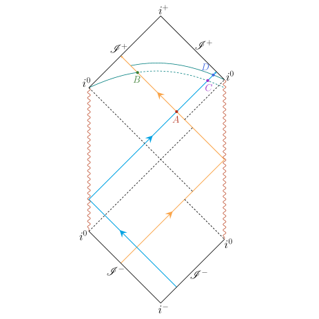
Figure 1: Penrose diagram depicting the shock wave FSC geometry. Here the lower (upper) part of the diagram corresponds to a contracting (expanding) universe. The probe is sent out from $\mathscr{I}^{-}$ and after a reflection at the singularity (wiggly line) emerges from the cosmological horizon (dashed line) where it intersects with the signal very close to the horizon at point $A$ and with the surface $\tau=\tau_{c}$ at point $B$. Without taking backreactions into account the signal intersects the surface $\tau=\tau_{c}$ at the point $C$. Taking backreactions into account the observer $O^{\prime}$ gets shifted to the point $D$ in order to still be able to receive the signal at $\tau=\tau_{c}$.

An observer $O$ located in the expanding region of the FSC receives this left-moving signal at a time $\tau_{c}$ and at a point $B=(x_{1},\tau_{c},\phi_{1})$ and eventually sees it moving towards future null infinity ($\mathscr{I}^{+}$). Due to the infinite blue shift at the past cosmological horizon the perturbation $(\delta M,\delta J)$ effectively causes the formation of a shock-wave geometry in an FSC background. A right-moving null signal crosses the worldline of the probe very close to the horizon at a point $A=(x_{\epsilon},\tau_{\epsilon},\phi_{\epsilon})$, where $\tau_{\epsilon}=\tau_{0}(1+\epsilon)$ for $1\gg\epsilon>0$, and intersects the $\tau=\tau_{c}$ surface at $C=(x_{2},\tau_{c},\phi_{2})$ in the unperturbed geometry where we place a second observer $O^{\prime}$. Due to the backreaction of the probe this observer gets shifted to a different spatial point $({\tilde{x}}_{2},{\tilde{\phi}}_{2})$ on the constant $\tau_{c}$ surface. Below we show that the comoving distance by which the observer $O^{\prime}$ is shifted due to the backreaction of the shock wave grows exponentially with the initial comoving distance between the observers $O$ and $O^{\prime}$, with a numerical prefactor corresponding to the holographic Lyapunov exponent.

Applying (24) to the spatial separation of comoving coordinates between the events $A$ and $B$ [$x_{1}-x_{\epsilon}=-H(\tau_{\epsilon},\tau_{c})$, $\phi_{1}-\phi_{\epsilon}=-G(\tau_{\epsilon},\tau_{c})$] and between the events $A$ and $C$ [$x_{2}-x_{\epsilon}=H(\tau_{\epsilon},\tau_{c})$, $\phi_{2}-\phi_{\epsilon}=G(\tau_{\epsilon},\tau_{c})$] yields

$$\Delta x=x_{2}-x_{1}=2H(\tau_{\epsilon},\tau_{c}),\qquad\;\Delta\phi=2G(\tau_{\epsilon},\tau_{c})\,.$$ (26)

Solving the integrals (25) for $e^{-\tau_{c}/\tau_{0}}\gg\epsilon>\delta\tau_{0}/\tau_{0}$ and $\tau_{c}\gg\tau_{0}$ gives the leading order behavior of the separation

$$\Delta x=\frac{\beta}{2\pi}\log{\frac{1}{\epsilon}}+\ldots\,,\qquad\Delta\phi=\frac{\mu\beta}{2\pi}\log{\frac{1}{\epsilon}}+\ldots\,,$$ (27)

expressed in terms of inverse Hawking temperature $\beta=2\pi\tau_{0}/\tau_{+}^{2}$ and angular velocity $\mu=\tau_{+}/\tau_{0}$. To leading order, $\Delta\phi=\mu\Delta x$ and therefore, in what follows we display only $\Delta x$.

A key aspect of (27) is that the spatial intervals are dominated by the red-shift factor $\epsilon$. Holographically, chaos is a consequence of this red-shift factor and backreaction effects from the shock-wave, which together produce an exponential dependence on the separation $\Delta x$, the prefactor of which is the Lyapunov exponent. To determine this exponent, we consider backreactions.

Backreaction and holographic Lyapunov exponent. Backreactions of the shock wave on the FSC background are included by modifying the original FSC parameters $m$ and $j$ to $\tilde{m}=m+\delta m$ and $\tilde{j}=j+\delta j$. As a consequence, the location of the event horizon also changes to $\tau_{0}\rightarrow\tau_{0}+\delta\tau_{0}$ where $\delta\tau_{0}=\frac{\beta}{2\pi}\,(\mu\,\delta j-\frac{1}{2}\,\delta m)$. This is the first law of thermodynamics for the FSC geometry,

$$-T\,\delta S=\delta M-\mu\,\delta J\,,\qquad\delta S:=\frac{\delta(\textrm{area})}{4G}=\frac{\pi\delta\tau_{0}}{2G}\,,$$ (28)

featuring a well-documented sign [36, 39]. The entropy change ${\delta}S$ concurs with the Bekenstein–Hawking area law.

Due to the backreaction of the shock wave on the FSC geometry the spatial interval $\Delta x=x_{j}-x_{i}$ changes

$$\tilde{x}_{j}-\tilde{x}_{i}=\pm\int\limits_{\tau_{i}}^{\tau_{j}}\frac{d\tau}{\tilde{f}(\tau)}:=\pm\tilde{H}(\tau_{i},\tau_{j}),$$ (29)

Here $\tilde{f}(\tau)=f(\tau)|_{m\rightarrow\tilde{m},j\rightarrow\tilde{j}}$. To linear order in $(\delta m,\delta j)$

$$\tilde{H}(\tau_{i},\tau_{j})=H-\delta m\int\limits_{\tau_{i}}^{\tau_{j}}\frac{d\tau}{f(\tau)^{2}}+2j\,\delta j\int\limits_{\tau_{i}}^{\tau_{j}}\frac{d\tau}{\tau^{2}f(\tau)^{2}}\,.$$ (30)

The above is valid for general probes carrying energy and angular momentum. Probes without angular momentum, i.e., null geodesics with $L=0$ don’t change the total angular momentum of the FSC and thus we have $\delta j=0$ and an expanding cosmological horizon in the expanding universe as depicted in Figure 1.

The results (29), (30) yield the interval

$$\tilde{x}_{2}-x_{\epsilon}=\tilde{H}(\tau_{\epsilon},\tau_{c})=x_{2}-x_{\epsilon}-\delta m\int\limits_{\tau_{\epsilon}}^{\tau_{c}}\frac{d\tau}{f(\tau)^{2}}\,.$$ (31)

Shifting $x_{2}\to{\tilde{x}}_{2}$ takes care of the necessary shift of $O^{\prime}$ so that the signal is still received at $\tau_{c}$. The crossing point $x_{\epsilon}$ remains the same as before since the correction to this point is subleading in perturbation parameters. Evaluating (31), the leading order contribution to the spatial shift of the observer,

$$\tilde{x}_{2}-x_{2}\approx\frac{\beta\delta\tau_{0}}{4\pi\tau_{0}\epsilon}=\frac{\beta}{4\pi}\,(\delta\log{S})\,e^{\frac{2\pi}{\beta}(x_{2}-x_{1})}\,,$$ (32)

contains the entropy change $\delta S$ given in (28). The results above can also be expressed in a coordinate-independent way in terms of proper distances [53], but we choose a simplified route to match with our field theory answers.

The expression (32) has the same functional form as the amplitude (Non-Lorentzian Chaos and Cosmological Holography) computed previously using field theory methods. To connect these results we first take $\tau_{c}$ to be large, thereby placing the observers $O$ and $O^{\prime}$ close to $\mathscr{I}^{+}$ where the holographic CCFT is encoded. Since (32) does not explicitly depend on $\tau_{c}$, this expression also holds close to $\mathscr{I}^{+}$. The inverse Hawking temperature $\beta$ can also be interpreted as the periodicity of the Euclidean time circle and hence the (inverse) temperature that an observer in the dual field theory measures. Thus, we find the holographic Lyapunov exponent

$$\lambda_{L}=\frac{2\pi}{\beta}\,,$$ (33)

in precise agreement with (18).

Outlook. Our results in this work have moved us into uncharted territories. We generalized 2d CFT results of chaos to non-Lorentzian settings. By studying spatial displacements in cosmological shock-wave solutions, we obtained a holographic Lyapunov exponent matching our field theory results. We shall address further aspects and generalizations of this work in [53]. We close with an important future direction. Chaos is related to the spreading of entanglement [54, 55]. Entanglement in Galilean and Carrollian CFTs was studied extensively in [44, 56, 28, 57, 58, 59]. We would like to understand how our results can help clarify the spread of entanglement and the speed of entanglement (dubbed ‘butterfly velocity’) in these non-Lorentzian theories.

Acknowledgements. We thank Jordan Cotler, Diptarka Das, Shahar Hadar, Elizabeth Himwich, Kristan Jensen, Daniel Kapec, Alexandru Lupsasca, Rohan Poojary, Stefan Prohazka, Jakob Salzer, Joan Simón, Douglas Stanford, and Andy Strominger for delightful scientific discussions and comments.

AB is partially supported by a Swarnajayanti Fellowship of the Department of Science and Technology (DST) and the Science and Engineering Research Board (SERB), India. DG is supported by the Austrian Science Fund (FWF), projects P 30822, P 32581, and P 33789. The research of MR is supported by the European Union’s Horizon 2020 research and innovation programme under the Marie Skłodowska-Curie grant agreement No. 832542 as well as the DOE grant de-sc/0007870. BR was supported in part by the INSPIRE scholarship of the Department of Science and Technology, Government of India, and the Long Term Visiting Students Program of the International Centre for Theoretical Sciences Bangalore. SC is partially supported by the ISIRD grant 9-252/2016/IITRPR/708.

References

- [1] E. Lorenz, “Predictibility.” Talk presented at the 139th AAAS meeting, 1972.
- [2] A. Bagchi and R. Gopakumar, “Galilean Conformal Algebras and AdS/CFT,” JHEP 07 (2009) 037, 0902.1385.
- [3] H. Bacry and J. Levy-Leblond, “Possible kinematics,” J. Math. Phys. 9 (1968) 1605–1614.
- [4] P. Di Francesco, P. Mathieu, and D. Senechal, Conformal Field Theory. Springer, 1997.
- [5] A. Bagchi, J. Chakrabortty, and A. Mehra, “Galilean Field Theories and Conformal Structure,” JHEP 04 (2018) 144, 1712.05631.
- [6] A. Bagchi, R. Gopakumar, I. Mandal, and A. Miwa, “GCA in 2d,” JHEP 08 (2010) 004, 0912.1090.
- [7] D. A. Roberts and D. Stanford, “Two-dimensional conformal field theory and the butterfly effect,” Phys. Rev. Lett. 115 (2015), no. 13, 131603, 1412.5123.
- [8] A. L. Fitzpatrick, J. Kaplan, and M. T. Walters, “Virasoro Conformal Blocks and Thermality from Classical Background Fields,” JHEP 11 (2015) 200, 1501.05315.
- [9] E. Perlmutter, “Bounding the Space of Holographic CFTs with Chaos,” JHEP 10 (2016) 069, 1602.08272.
- [10] A. Bagchi and R. Fareghbal, “BMS/GCA Redux: Towards Flatspace Holography from Non-Relativistic Symmetries,” JHEP 10 (2012) 092, 1203.5795.
- [11] C. Duval, G. W. Gibbons, P. A. Horvathy, and P. M. Zhang, “Carroll versus Newton and Galilei: two dual non-Einsteinian concepts of time,” Class. Quant. Grav. 31 (2014) 085016, 1402.0657.
- [12] A. Bagchi, R. Basu, A. Kakkar, and A. Mehra, “Flat Holography: Aspects of the dual field theory,” JHEP 12 (2016) 147, 1609.06203.
- [13] A. Bagchi, R. Basu, A. Mehra, and P. Nandi, “Field Theories on Null Manifolds,” JHEP 02 (2020) 141, 1912.09388.
- [14] A. Bagchi, “Correspondence between Asymptotically Flat Spacetimes and Nonrelativistic Conformal Field Theories,” Phys. Rev. Lett. 105 (2010) 171601, 1006.3354.
- [15] L. Cornalba and M. S. Costa, “A New cosmological scenario in string theory,” Phys. Rev. D 66 (2002) 066001, hep-th/0203031.
- [16] L. Cornalba and M. S. Costa, “Time dependent orbifolds and string cosmology,” Fortsch. Phys. 52 (2004) 145–199, hep-th/0310099.
- [17] S. H. Shenker and D. Stanford, “Black holes and the butterfly effect,” JHEP 03 (2014) 067, 1306.0622.
- [18] S. H. Shenker and D. Stanford, “Multiple Shocks,” JHEP 12 (2014) 046, 1312.3296.
- [19] J. Maldacena, S. H. Shenker, and D. Stanford, “A bound on chaos,” JHEP 08 (2016) 106, 1503.01409.
- [20] A. Larkin and Y. Ovchinnikov, “Quasiclassical method in the theory of superconductivity,” Sov.Phys.JETP 28 (19669) 1200.
- [21] D. A. Roberts, D. Stanford, and L. Susskind, “Localized shocks,” JHEP 03 (2015) 051, 1409.8180.
- [22] S. H. Shenker and D. Stanford, “Stringy effects in scrambling,” JHEP 05 (2015) 132, 1412.6087.
- [23] A. Kitaev, “Hidden Correlations in the Hawking Radiation and Thermal Noise,” talk given at KITP, Santa Barbara (2014). http://online.kitp.ucsb.edu/online/joint98/kitaev/.
- [24] F. M. Haehl, R. Loganayagam, P. Narayan, and M. Rangamani, “Classification of out-of-time-order correlators,” SciPost Phys. 6 (2019), no. 1, 001, 1701.02820.
- [25] The approximation of large central charge corresponds to the classical approximation on the gravity side (small Newton constant) [47], whenever there is a gravity dual. Therefore, this approximation is not only convenient, it is also pertinent to the holographic calculation in the second half of our work.
- [26] A. Bagchi, M. Gary, and Zodinmawia, “Bondi-Metzner-Sachs bootstrap,” Phys. Rev. D 96 (2017), no. 2, 025007, 1612.01730.
- [27] A. Bagchi, M. Gary, and Zodinmawia, “The nuts and bolts of the BMS Bootstrap,” Class. Quant. Grav. 34 (2017), no. 17, 174002, 1705.05890.
- [28] E. Hijano and C. Rabideau, “Holographic entanglement and Poincaré blocks in three-dimensional flat space,” JHEP 05 (2018) 068, 1712.07131.
- [29] E. Hijano, “Semi-classical BMS3 blocks and flat holography,” JHEP 10 (2018) 044, 1805.00949.
- [30] W. Merbis and M. Riegler, “Geometric actions and flat space holography,” JHEP 02 (2020) 125, 1912.08207.
- [31] Since has a physical dimension a more precise definition of scrambling time is , where is either or , depending on which weight is bigger. However, since we assume the weights to be finite and to be large, the quantity must be large and hence dominates the scrambling time.
- [32] This result can be extended to the case where since a non-zero only affects the terms.
- [33] J. M. Maldacena, “The Large N limit of superconformal field theories and supergravity,” Adv. Theor. Math. Phys. 2 (1998) 231–252, hep-th/9711200.
- [34] G. Barnich, A. Gomberoff, and H. A. Gonzalez, “The Flat limit of three dimensional asymptotically anti-de Sitter spacetimes,” Phys. Rev. D 86 (2012) 024020, 1204.3288.
- [35] A. Bagchi, S. Detournay, and D. Grumiller, “Flat-Space Chiral Gravity,” Phys. Rev. Lett. 109 (2012) 151301, 1208.1658.
- [36] A. Bagchi, S. Detournay, R. Fareghbal, and J. Simón, “Holography of 3D Flat Cosmological Horizons,” Phys. Rev. Lett. 110 (2013), no. 14, 141302, 1208.4372.
- [37] G. Barnich, “Entropy of three-dimensional asymptotically flat cosmological solutions,” JHEP 10 (2012) 095, 1208.4371.
- [38] G. Barnich, A. Gomberoff, and H. A. González, “Three-dimensional Bondi-Metzner-Sachs invariant two-dimensional field theories as the flat limit of Liouville theory,” Phys. Rev. D 87 (2013), no. 12, 124032, 1210.0731.
- [39] A. Bagchi, S. Detournay, D. Grumiller, and J. Simon, “Cosmic Evolution from Phase Transition of Three-Dimensional Flat Space,” Phys. Rev. Lett. 111 (2013), no. 18, 181301, 1305.2919.
- [40] H. Afshar, A. Bagchi, R. Fareghbal, D. Grumiller, and J. Rosseel, “Spin-3 Gravity in Three-Dimensional Flat Space,” Phys. Rev. Lett. 111 (2013), no. 12, 121603, 1307.4768.
- [41] H. A. Gonzalez, J. Matulich, M. Pino, and R. Troncoso, “Asymptotically flat spacetimes in three-dimensional higher spin gravity,” JHEP 09 (2013) 016, 1307.5651.
- [42] R. Fareghbal and A. Naseh, “Flat-Space Energy-Momentum Tensor from BMS/GCA Correspondence,” JHEP 03 (2014) 005, 1312.2109.
- [43] S. Detournay, D. Grumiller, F. Schöller, and J. Simón, “Variational principle and one-point functions in three-dimensional flat space Einstein gravity,” Phys. Rev. D 89 (2014), no. 8, 084061, 1402.3687.
- [44] A. Bagchi, R. Basu, D. Grumiller, and M. Riegler, “Entanglement entropy in Galilean conformal field theories and flat holography,” Phys. Rev. Lett. 114 (2015), no. 11, 111602, 1410.4089.
- [45] A. Bagchi, D. Grumiller, and W. Merbis, “Stress tensor correlators in three-dimensional gravity,” Phys. Rev. D 93 (2016), no. 6, 061502, 1507.05620.
- [46] J. Hartong, “Holographic Reconstruction of 3D Flat Space-Time,” JHEP 10 (2016) 104, 1511.01387.
- [47] G. Barnich and G. Compere, “Classical central extension for asymptotic symmetries at null infinity in three spacetime dimensions,” Class. Quant. Grav. 24 (2007) F15–F23, gr-qc/0610130.
- [48] M. Bañados, C. Teitelboim, and J. Zanelli, “The Black hole in three-dimensional space-time,” Phys. Rev. Lett. 69 (1992) 1849–1851, hep-th/9204099.
- [49] M. Bañados, M. Henneaux, C. Teitelboim, and J. Zanelli, “Geometry of the (2+1) black hole,” Phys. Rev. D 48 (1993) 1506–1525, gr-qc/9302012. [Erratum: Phys.Rev.D 88, 069902 (2013)].
- [50] J. Engelsöy, T. G. Mertens, and H. Verlinde, “An investigation of AdS2 backreaction and holography,” JHEP 07 (2016) 139, 1606.03438.
- [51] D. Grumiller and R. McNees, “Universal flow equations and chaos bound saturation in 2d dilaton gravity,” JHEP 01 (2021) 112, 2007.03673.
- [52] The case yields essentially the same results and will be addressed in upcoming work [53].
- [53] A. Bagchi, S. Chakrabortty, D. Grumiller, B. Radhakrishnan, M. Riegler, and A. Sinha, “Chaos and holography in BMS invariant field theories.” in preparation.
- [54] M. Mezei and D. Stanford, “On entanglement spreading in chaotic systems,” JHEP 05 (2017) 065, 1608.05101.
- [55] M. Mezei, “On entanglement spreading from holography,” JHEP 05 (2017) 064, 1612.00082.
- [56] H. Jiang, W. Song, and Q. Wen, “Entanglement Entropy in Flat Holography,” JHEP 07 (2017) 142, 1706.07552.
- [57] L. Apolo, H. Jiang, W. Song, and Y. Zhong, “Modular Hamiltonians in flat holography and (W)AdS/WCFT,” JHEP 09 (2020) 033, 2006.10741.
- [58] D. Grumiller, P. Parekh, and M. Riegler, “Local quantum energy conditions in non-Lorentz-invariant quantum field theories,” Phys. Rev. Lett. 123 (2019), no. 12, 121602, 1907.06650.
- [59] V. Godet and C. Marteau, “Gravitation in flat spacetime from entanglement,” JHEP 12 (2019) 057, 1908.02044.