Variational Causal Networks: Approximate Bayesian Inference over Causal Structures

Abstract

Learning the causal structure that underlies data is a crucial step towards robust real-world decision making. The majority of existing work in causal inference focuses on determining a single directed acyclic graph (DAG) or a Markov equivalence class thereof. However, a crucial aspect to acting intelligently upon the knowledge about causal structure which has been inferred from finite data demands reasoning about its uncertainty. For instance, planning interventions to find out more about the causal mechanisms that govern our data requires quantifying epistemic uncertainty over DAGs. While Bayesian causal inference allows to do so, the posterior over DAGs becomes intractable even for a small number of variables. Aiming to overcome this issue, we propose a form of variational inference over the graphs of Structural Causal Models (SCMs). To this end, we introduce a parametric variational family modelled by an autoregressive distribution over the space of discrete DAGs. Its number of parameters does not grow exponentially with the number of variables and can be tractably learned by maximising an Evidence Lower Bound (ELBO). In our experiments, we demonstrate that the proposed variational posterior is able to provide a good approximation of the true posterior.

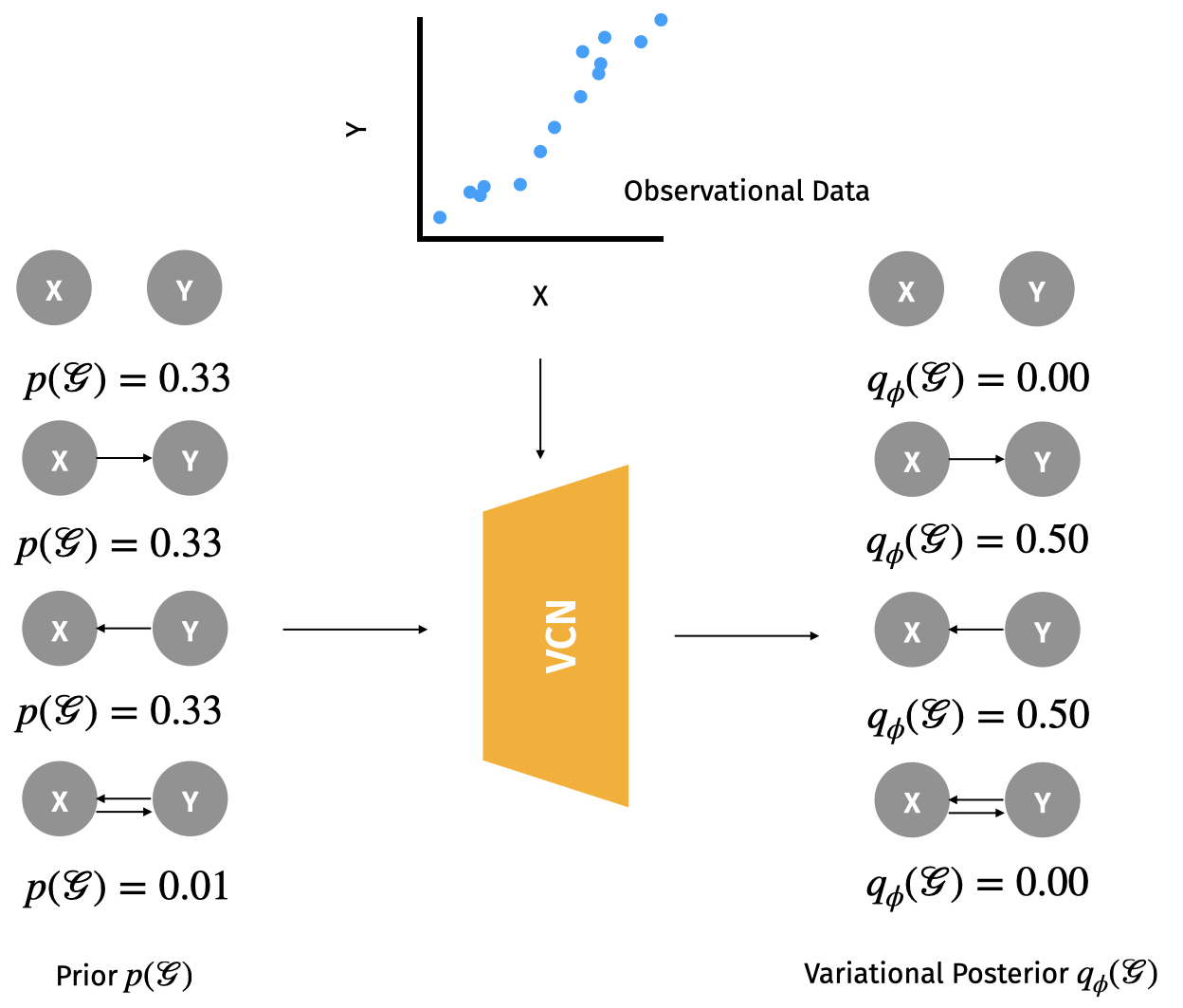
Figure 1: Schematic Diagram of Variational Inference on SCMs with VCN.

Moving from learning correlation and association in data to causation is a critical step towards increased robustness, interpretability and real-world decision-making [27, 34]. Doing so entails learning the causal structure underlying the data generating process. Causal inference is concerned with determining the causal structure of a set of random variables from data, commonly represented as a directed acycilc graph (DAG) [29]. While Structural Causal Models (SCMs) provide a generative model over the data, they are hard to learn from data due to the non-identifiability of the causal models without interventional data [7] and the combinatorial nature of the space of DAGs [15]. Even with infinite amount of data, recovering the causal structure is intrinsically hard since a DAG is only identifiable up to its Markov equivalence class (MEC) and the space of possible DAGs grows super-exponentially with the number of variables. While the majority of work on causal inference [6, 5, 38] deals with getting a single underlying causal structure without a probabilistic treatment, quantifying the epistemic uncertainty in case of non-identifiability is crucial and is not possible in these approaches.

In this work, we take a Bayesian approach to causal structure learning. Given only finite observational data, a Bayesian approach allows us to quantify the uncertainty in the causal structure of the data generating process, even before performing interventions. Having such a framework over causal structures can help further downstream tasks on graph learning and causal inference. For example, we can leverage the model’s uncertainty to select informative interventions and discover the full graph with minimal amount of interventions [2]. Also, for estimating the causal effect of certain variables, it is often not required to know the full graph. Hence, by marginalising the posterior we can uncover the confidence we have about a specific causal effect, which may already fall below a specified tolerance level. Having such a model is very desirable as interventions are hard to perform, sometimes unethical and even impossible [29].

A key component in learning causal structures is the identifiability under the availability of observational data. While some assumptions are always required to say anything about the underlying causal process, additional assumptions are sometimes made to especially make the causal model identifiable from (observational) data. These additional assumptions are not necessarily part of the data generating process, and hence the recovered causal structure may be incorrect due to model misspecification. In addition, identifiability results are usually asymptotic in the number of samples. Causal discovery in a limited sample regime calls for active learning to perform interventions to improve identifiability. Such setups benefit from probabilistic reasoning about unknown causal structures. We are interested in such settings and we propose a Bayesian framework for linear SCM’s with additive noise which can quantify the uncertainty in the learned causal structure.

Our contributions are as follows:

• We perform Bayesian inference over the unknown causal structures. The posterior over this distribution is intractable. Therefore, we perform variational inference and demonstrate how we can model the variational family over this distribution.

• The key contribution is to model distributions over adjacency matrices of the causal structures with an autoregressive distribution using an LSTM.

• Empirically demonstrate the performance of our modeling choice.

• Evaluating Bayesian causal inference techniques are hard in practice. We discuss the difficulty entailed in evaluation, as well as provide insights which alleviate this problem.

1 Problem Setting

Causal modeling

Consider a set of $d$ random variables $\mathbf{X}:=\{X_{1},\dots,X_{d}\}$. A Structural Causal Model (SCM) [29] over $\mathbf{X}$ is defined as set of structural assignments

$$X_{i}:=f_{i}(\mathbf{x}_{\pi_{\mathcal{G}}(i)},\epsilon_{i})~{},i=1,...,d$$ (1)

corresponding to a Directed Acyclic Graph (DAG) $\mathcal{G}$ with vertices $\mathbf{X}$. In here, $\pi_{\mathcal{G}}(i)$ are the parents of $X_{i}$ in $\mathcal{G}$, $\epsilon_{i}$ are independent noise variables with probability density $P_{\epsilon_{i}}$ and the $f_{i}$’s are (potentially non-linear) functions. The SCM entails a joint probability distribution $P_{\mathbf{x}}$ over the random variables. In this work, we assume that all the endogenous variables are observed, that is, there are no hidden confounders.

A popular instantiation of this generic framework are linear SCMs with additive noise, given by:

$$x_{i}:=\bm{\theta}_{i}^{T}\mathbf{x}_{\pi_{\mathcal{G}}(i)}+\epsilon_{i}~{}~{}~{}~{}\bm{\theta}_{i}\in\mathbb{R}^{|\pi_{\mathcal{G}}(i)|}$$ (2)

wherein $\bm{\theta}_{i}$ are parameters (edge weights) of the linear functions $f_{i}$. Alternatively, this can be written as

$$x_{i}:=\bm{\theta}_{i}^{T}\left(\mathbf{X}\circ\mathbf{A}_{\mathcal{G}_{i}}\right)+\epsilon_{i}~{}~{}~{}~{}\bm{\theta}_{i}~{},~{}\mathbf{A}_{\mathcal{G}_{i}}\in\mathbb{R}^{d}~{},$$ (3)

where $\circ$ corresponds to elementwise product, $\mathbf{A}_{\mathcal{G}_{i}}$ is the $i$^th row of $\mathbf{A}_{\mathcal{G}}\in\mathbb{R}^{d\times d}$, the $(0,1)$-adjacency matrix of $\mathcal{G}$. We restrict our further exposition to continuous random variables. However, the framework presented in the remainder of the paper applies to discrete random variables as well. We focus on linear SCMs with Gaussian variables, as they are non-identifiable in this setting and hence obtaining uncertainty estimates is useful. Non-linear additive noise SCM’s with Gaussian variables are identifiable, and hence a single point estimate suffices.

NOTEARS - Causal inference as continuous optimization problem

In practice, we often have data while the causal structure that underlies the data generating process is unknown to us. Causal discovery is concerned with recovering this causal structure, e.g. in the form of an SCM, from observational data or interventional data (or both). Assuming a linear SCM, this coincides with estimating the graph $\mathcal{G}$, i.e. its adjacency matrix $\mathbf{A}$, and its corresponding edge weights $\bm{\theta}=\{\bm{\theta}_{1},...,\bm{\theta}_{d}\}$, given data ${\mathcal{D}}:=\{\mathbf{x}_{1},...,\mathbf{x}_{n}\}\in{\mathcal{X}}^{n}$.

In score-based causal discovery, we use a score function $F:\{0,1\}^{d\times d}\times{\mathcal{X}}^{n}\mapsto\mathbb{R}$ to find the graph that best corresponds to the data as follows:

$$\operatorname*{arg\,min}_{\mathbf{A}\in\{0,1\}^{d\times d}}F(\mathbf{A},{\mathcal{D}})\quad\text{s.t.}~{}~{}{\mathcal{G}}(\mathbf{A})\in\operatorname{DAG}(d)$$ (4)

where $\mathbf{A}$ is the $\{0,1\}$ adjacency matrix of graph ${\mathcal{G}}$.

However, since the search space of DAGs of this combinatorial optimization problem grows in the order of $\mathcal{O}(2^{d^{2}})$, solving (4) becomes infeasible even for a relatively small number of variables $d$.

Addressing this issue, Zheng et al. [38] propose an alternative formulation that converts the combinatorial problem into the following continuous program:

$$\operatorname*{arg\,min}_{{\bm{W}}\in\mathbb{R}^{d\times d}}F({\bm{W}},{\mathcal{D}})\quad\text{s.t.}~{}~{}\text{tr}\left(e^{{\bm{W}}}\right)-d=0~{}.$$ (5)

that can be solved with standard tools of constrained optimization such as the Lagrange method. In here, we have converted the adjacency matrix $\mathbf{A}\in\{0,1\}^{d\times d}$ into a weighted adjacency matrix ${\bm{W}}\in\mathbb{R}^{d\times d}$ such that $a_{i,j}=1\Leftrightarrow w_{i,j}\neq 0$.

Bayesian inference over DAGs

An important aspect towards acting intelligently upon the knowledge about the causal structure which has been inferred from finite data demands reasoning about its uncertainty. For instance, in scientific inquiry, planning interventional experiments to find out more about the causal mechanisms that govern a data-generating system of interest requires quantifying epistemic uncertainty over DAGs. Bayesian inference gives us a principled framework for the treatment of such uncertainty (Figure 1).

In the Bayesian framework, we encode our prior structural knowledge in form of a prior $p({\mathcal{G}})$ over DAGs. By combining the prior with the likelihood $p({\mathcal{D}}|{\mathcal{G}})$ through Bayes’ rule, we obtain a posterior distribution over DAGs:

$$p(\mathcal{G}|{\mathcal{D}})=\frac{p({\mathcal{D}}|\mathcal{G})p(\mathcal{G})}{p({\mathcal{D}})}$$ (6)

where $p({\mathcal{D}})=\sum_{\mathcal{G}}\int_{\theta}p(\mathbf{x}|\mathcal{G},\bm{\theta})p(\bm{\theta}|\mathcal{G})p(\mathcal{G})d\bm{\theta}$ is the model evidence. A key issue with (6) is the intractable evidence term in the denominator. Even if the integral over $\bm{\theta}$ can be solved analytically such as in the case of linear structural equations with Gaussian prior and likelihood with standard parameter priors [10], the sum over possible DAGs grows in the order of ${\mathcal{O}}(2^{d^{2}})$, making its computation infeasible even for a small number of variables $d$.

2 Variational Causal Networks

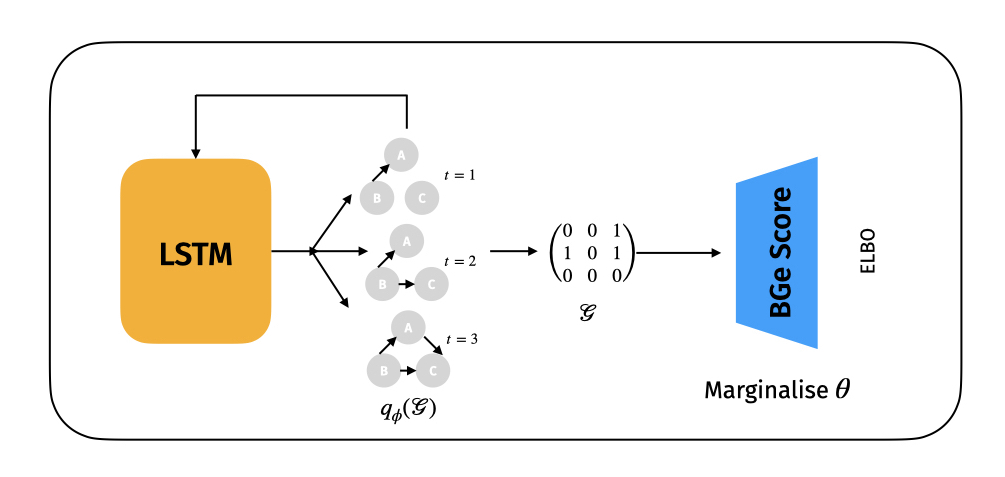
Figure 2: Schematic Diagram of Variational Causal Networks

In this section, we present our variational inference (VI) framework for approximating Bayesian posteriors over causal structures (Equation 6). First, we derive the evidence lower bound and sketch out how to perform VI on DAGs. Unlike the variational inference in a latent variable model [4], the evidence lower bound is still intractable in the case of causal models due to the superexponential number of graph configurations. Therefore, we introduce a novel parametric variational family which makes the intractable ELBO into a tractable one while still having the flexibility to model complex distributions over DAGs. Such a variational family can be modelled using autoregressive models like LSTM [17]. This particular instantiation of approximate Bayesian inference for SCMs with the presented variational family is called Variational Causal Networks (VCN).

2.1 Variational Inference for Causal Structures

In variational inference [4], we aim to approximate the Bayesian posterior $p(\mathcal{G}|{\mathcal{D}})$ by a variational distribution $q_{\phi}({\mathcal{G}})$, parameterized by $\phi$, that has a tractable density. To learn the parameters of our variational distribution, we minimize the KL-Divergence between $q_{\phi}(\mathcal{G})$ and the true posterior $p(\mathcal{G}|{\mathcal{D}})$ which is equivalent to maximising the Evidence Lower Bound (ELBO), given by the following proposition.

Proposition 1.

(ELBO) Let $q_{\phi}(\mathcal{G})$ be the variational posterior over causal structures. Then the evidence lower bound (ELBO) is given by:

$$\begin{split}\log p({\mathcal{D}})\geq\mathcal{L}(\phi;{\mathcal{D}})=\mathop{{}\mathbb{E}}_{q_{\phi}(\mathcal{G})}\left[\log p({\mathcal{D}}|\mathcal{G})\right]-\operatorname{D_{KL}}\left(q_{\phi}(\mathcal{G})||p(\mathcal{G})\right)\end{split}$$ (7)

To maximise the ELBO, we estimate the gradients $\nabla_{(\phi)}\mathcal{L}(\phi;{\mathcal{D}})$ to employ a form of gradient ascent on the objective.

2.2 A Variational Family for Causal Structures

A key challenge to variational inference over DAGs concerns the choice of the variational distribution $q_{\phi}(\mathcal{G})$ over discrete DAGs ${\mathcal{G}}$. For instance, if we choose $q_{\phi}({\mathcal{G}})$ naively as categorical distribution over the space of DAGs, the dimensionality of $\phi$ grows super-exponentially in the number of variables $d$ (i.e. $\mathcal{O}(2^{d^{2}})$), rendering this choice impractical. Hence, we need to find a way of representing $q_{\phi}({\mathcal{G}})$ that is not combinatorial in its nature while ensuring a rich family of distributions over graphs. In addition, to be able to compute Monte Carlo gradient estimates of the ELBO in (7), $q_{\phi}(\mathcal{G})$ needs to have a tractable probability density.

Aiming to fulfil these requirements, we represent graphs by their adjacency matrix $\mathbf{A}\in\{0,1\}^{d\times d}$ and model $q_{\phi}$ as a discrete distribution over such $\{0,1\}$-matrices. While Ke et al. [19] represent each entry of the adjacency matrix as independent Bernoulli variable, such approach is insufficient to capture any dependencies between the entries of the adjacency matrix which are necessary to ensure that $q(\mathbf{A})$ only assigns positive probabilities to adjacency matrices corresponding to DAGs. For instance, to avoid cycles of length two, $(\mathbf{A})_{i,j}$ needs to have a strong negative dependency $(\mathbf{A})_{j,i}$, i.e., if there is a directed edge $i\rightarrow j$ there must be no edge $j\rightarrow i$, and reverse. In addition, a factorisable distribution can only capture unimodal distributions while the posterior over causal structures in the non-identifiable case could have exponential number of modes. Hence, the variational distribution needs to be parameterised such that multiple modes could be captured. In order to address these issues, we model this discrete distribution as an autoregressive distribution over entries of the adjacency matrix using an LSTM [17].

Let $q_{\phi}(\mathcal{G})=q_{\phi}(\mathbf{A}_{\mathcal{G}})$ be defined in an autoregressive manner as follows:

$$\begin{split}q_{\phi}(\mathbf{A}_{\mathcal{G}})&=\prod_{i=1}^{d(d-1)}q_{\phi}(a_{\mathcal{G}_{i}}|a_{\mathcal{G}_{1:i-1}})\\ s.t.~{}~{}~{}~{}q_{\phi}(a_{\mathcal{G}_{i}}|a_{\mathcal{G}_{1:i-1}})&:=\text{Bernoulli}\left(a_{\mathcal{G}_{i}};f_{\phi}\left(a_{\mathcal{G}_{1:i-1}}\right)\right),~{}~{}\mathbf{A}_{\mathcal{G}}=\{a_{\mathcal{G}_{i}}\}_{i=1}^{d(d-1)}\end{split}$$

where only the non-diagonal elements of the adjacency matrix are modelled and $f_{\phi}$ is a function which predicts the Bernoulli parameter based on the previous realisations of the entries of the adjacency matrix, thus making the distribution autoregressive. We model this function using an LSTM [17].

Note that using an autoregressive distribution on the entries of the adjacency matrix helps to implicitly keep a distribution over super-exponential number of graphs, and also be able to sample from that distribution.

Prior over graph structures

Choosing the appropriate prior $p(\mathcal{G})$ over graph structures is important to learn good approximation of the posterior. In causal discovery, it is usually a requirement that the search space of all graphs is a DAG. However, in the parameterisation described above, the discrete distribution is defined over all possible graphs, including the one which contains cycles. Having support over graphs with cycles and using maximum likelihood estimation results in high probability mass corresponding to a fully connected graph in the approximate posterior. Therefore, appropriate DAG regularizers are required. We employ the result of NOTEARS [38] to define a Gibbs distribution as the prior which helps us to limit the support of graphs to just DAGs. We can also encode additional assumptions about the data generating process such as sparsity. The Gibbs distribution in this case could be defined as:

$$p(\mathcal{G})\propto\exp(-\lambda_{t}g(\mathbf{A}_{\mathcal{G}})-\lambda_{s}\norm{\mathbf{A}_{\mathcal{G}}}_{1})$$ (8)

where $g(\mathbf{A}_{\mathcal{G}})$ is the DAG constraint given by the matrix exponential [38], i.e $g(\mathbf{A}_{\mathcal{G}})=\tr\left[e^{\mathbf{A}_{\mathcal{G}}}\right]-d$. Matrix binomial can also be used to define $g$, as given in [37]. The second term in the Gibbs distribution corresponds to the sparsity constraint. $\lambda_{t}$ and $\lambda_{s}$ are tunable hyperparameters. Typically, $\lambda_{t}\to\infty$ if graphs with cycles should have zero probability mass under the posterior. However, any large value should still give a reasonable prior with very low probabilities for cyclic graphs.

Marginal Likelihood

We use standard parameter priors which ensure marginal likelihood $\log p({\mathcal{D}}|\mathcal{G})$ is ”score-equivalent”, i.e. all the DAGs which are in the same MEC have the same marginal likelihood. This can be ensured with a Gaussian-Wishart prior over the parameters $\bm{\theta}$ and the marginalisation can be done in closed form [10, 23] (called as the BGe score). Using this parameter prior to calculate marginal likelihood in the ELBO makes the ELBO score-equivalent. Details are given in Appendix B.3.

2.3 Estimating Gradients

Since the KL regulariser is defined on a discrete distribution with many parameters, obtaining a Monte Carlo estimate of this term (and hence the corresponding ELBO) requires unbiased gradients of $\phi$. Therefore, we use the score-function gradient estimator [36] with exponential moving average baseline for obtaining the gradients. As the score function estimator does not require the estimand function to be differentiable, we can perform closed form marginalisation of the parameters with the standard parameter priors like that of Gaussian-Wishart.

The detailed algorithm is given in Algorithm 1.

Algorithm 1 VCN Algorithm

1:$\phi\leftarrow$ initialise parameters

2:repeat

3:     Sample $L$ graphs $\{\mathcal{G}^{(i)}\}_{i=1}^{L}$ autoregressively from $q_{\phi}(\mathbf{A}_{\mathcal{G}})$ using an LSTM.

4:     Calculate the per-sample marginal log-likelihood $\log p({\mathcal{D}}|\mathcal{G}^{(i)})$ by marginalising $\bm{\theta}$ to obtain the BGe Score [10, 23].

5:     $g\leftarrow\frac{1}{L}\sum_{i=1}^{L}\nabla_{\phi}\left[\log p({\mathcal{D}}|\mathcal{G}^{(i)})-\left[\log q_{\phi}(\mathcal{G}^{(i)})-\log p(\mathcal{G}^{(i)})\right]\right]$

6:     $\phi\leftarrow$ Update parameters using gradients $g$.

7:until $\phi\leftarrow$ converge.

3 Related Work

Causal Discovery: Broadly, causal structure learning approaches can be mainly categorised to two different paradigms with regards to kind of data used: methods involving learning structure from purely observational data and methods involving learning structure from both observational and interventional data. Both these approaches strongly rely on the identifiability of SCM. Zheng et al. [38], Yu et al. [37], Lachapelle et al. [24] use a score-based objective with global search over DAG space to learn the structure. Lachapelle et al. [24] extend the linear model of [38] to non-linear case using neural networks. GES [6, 31] greedily searches over the space of CPDAG’s and maximize a score based on Bayesian Information Criterion (BIC). LiNGAM [33] uses an Independent Component Analysis (ICA) based approach by making the assumption that either the variables or one of the noise variables are non-Gaussian. PC [34] algorithm uses a constraint based approach for causal discovery.

Different from the above approaches, a few approaches use a combination of observational and interventional data to learn the causal structure [13]. ICP [28] assumes a linear SCM and resorts to conditional independence testing to test the hypothesis of invariance, a concept wherein the plausible causal predictors of a given variable are stable across different interventions. [16] extend ICP to non-linear SCMs. These methods do not infer the complete graph but instead just the causal parents of a particular variable. The difficulty of these approaches rest in the fact that conditional independence tests are hard to perform. More recently, [3, 20] and [19] use a meta-learning objective to learn the causal structure using interventional data.

Bayesian Approach to Structure Learning: Existing approaches for Bayesian learning of causal graphs are mainly concerned with efficient sampling of graph structures from the posterior distribution. A popular choice for such an approach is the Markov Chain Monte Carlo (MCMC) with suitably chosen energy functions and heuristics [8, 26, 25, 22, 14, 9]. While Niinimäki et al. [26] is concerned with causal discovery by sampling graph structures from partial orders of edge orientation, Madigan et al. [25] proposes an approach for learning probabilistic graphical models with discrete variables called as structure MCMC. Kuipers and Moffa [22], Grzegorczyk and Husmeier [12] and Ellis and Wong [8] propose improved MCMC techniques for sampling graph structures by restricting graph space to certain topology and sampling from a restricted space. Heckerman et al. [14] use a BIC based scoring function to learn a Bayesian network by sampling from Metropolis-Hastings under different energy configurations. An estimate of MAP is obtained using Maximum Likelihood to get the final graph structure. Agrawal et al. [2] use DAG bootstrapping to estimate the posterior over graphs and use this for budgeted experimental design for causal discovery. While all these techniques are intended for a Bayesian approach to structure learning, they face the problem of efficiently approximating the posterior over graph structures and hence resort to either heuristics or restricted graph structures. However, we do not make any simplifying assumptions about the graph structures and we can efficiently approximate the posterior while being able to sample exactly from them.

4 Experiments

To validate the modelling choice presented in the previous section, we perform experiments mainly focusing on the following aspects: (1) since we approximate the posterior, we evaluate how close is the approximation to the true posterior in lower dimensional settings ($\leq 4$) where enumeration of true posterior is possible. (2) We outline the difficulty involved in evaluating the Bayesian Causal inference models in higher dimensions where enumeration is not possible and suggest possible metrics which alleviate the problem and quantify how well the true posterior is approximated. We further evaluate our model on these metrics.

Key Findings

We summarise the experimental results as follows: (1) The proposed autoregressive approach of VCN performs better than a factorised distribution [19] in all the considered settings. This is due to the ability of an autoregressive distribution to model multi-modal posteriors as compared to the unimodal factorised distribution. (2) In higher dimensions, the proposed approach compares favourably to competitive baselines on various metrics. (3) VCN achieves a good approximation vs run-time trade-off, thus making it a suitable approach for Bayesian causal inference.

Experimental Settings

We evaluate our method on both synthetic and real datasets. For generating synthetic data, we follow the procedure of NOTEARS [38]. We sample a DAG at random from an Erdos-Renyi (ER) model with expected number of edges equal to $d$. Each reported result is over 20 different random graphs. The models were trained with a learning rate of $1e-2$ using the Adam optimiser [21] for 30k epochs. We consider the settings when we have $n=10,100$ samples. For taking the Monte Carlo estimate of the ELBO, we take $L=1000$ samples. $\lambda_{s}$ is fixed to 0.01 and $\lambda_{t}$ is annealed from 10 to 1000 with an exponential annealing schedule.

Baselines

Parameterising the posterior with a factorised distribution [19] is our main baseline as it involves differentiable causal learning based techniques similar to our approach. We also compare with DAG Bootstrap [2] where the posterior is estimated by bootstrapping the data with any causal discovery algorithm and then forming an empirical estimate of the posterior based on frequency count. We use LiNGAM [33] and NOTEARS [38] as underlying causal discovery algorithms for DAG Bootstrap. They are denoted by Boot Lingam and Boot Notears respectively. In addition, we compare with the MCMC approach of Minimal IMAP MCMC [1]. Details of experimental settings of each of these techniques is given in Appendix B.4.

4.1 Evaluation Metrics

For low dimensional variables $(d\leq 4)$, we can enumerate the true posterior for all graphs. Therefore, in this setting we compute the distance between the variational posterior learned from data and the true posterior.

For higher dimensional variables, where enumerating the true posterior is not possible, evaluating Bayesian causal inference algorithms is not straightforward. Directly comparing the likelihoods do not necessarily ensure that the posterior learned is good, as graphs with more edges always have higher likelihoods. Instead, we employ the following metrics:

Expected Structural Hamming Distance ($\mathop{{}\mathbb{E}}[\text{SHD}]$)

Given that the true posterior has modes over all the graphs inside the MEC corresponding to the ground truth graph, we can sample the graphs from the model and then compute the Structural Hamming Distance (SHD) between these samples and the ground truth. We can then compute the empirical mean of these SHDs as a metric. As all the graphs inside the MEC have the same number of edges, this metric indicates how well the approximated posterior is close to the ground truth on average. If $\mathcal{G}_{\text{GT}}$ is the ground truth data generating graph, then $\mathop{{}\mathbb{E}}[\text{SHD}]$ is given by

$$\mathop{{}\mathbb{E}}_{q_{\phi}(\mathcal{G})}[\text{SHD}]\approx\frac{1}{T}\sum_{i=1}^{T}\left[\text{SHD}(\mathcal{G}^{(i)},\mathcal{G}_{\text{GT}})\right]~{}~{}~{}~{}\mathcal{G}^{(i)}\sim q_{\phi}(\mathcal{G})$$ (9)

Area Under Reciever Operating Curve (AUROC)

If we care for just feature probabilities of quantities like the presence of an edge, we can compute edge beliefs and compute the Receiver Operating Curve (ROC). The area under this curve can be treated as a metric for evaluating the Bayesian model. However, it does not necessarily give a full picture of the multiple modes of the posterior and whether the sampled graph is far away /close to the MEC of the true graph. Nevertheless, it can still be informative of the edge beliefs of the learned approximation. Details of computing this is give in [30].

We would like to note that though these metrics capture to a reasonable extent how well the true posterior is approximated, they are still imperfect. Since the true posterior has mass over all the graphs corresponding to MEC of the ground truth graph, the true posterior does not necessarily evaluate to zero on $\mathop{{}\mathbb{E}}[\text{SHD}]$ and one on AUROC. Hence, evaluating the learned model on these metrics only partially indicates how well the true posterior is approximated.

4.2 Results

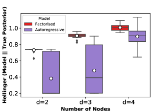
Figure 3: Hellinger distance of the full posterior of the approximation with the true posterior.

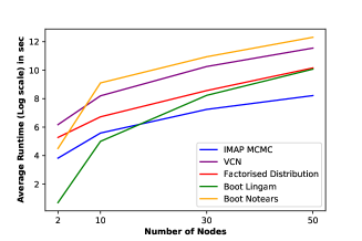
Figure 4: Average runtime (in seconds, log scale) of different Bayesian causal inference approaches.

4.2.1 Estimation of True Posterior

As indicated before, when the number of variables in the graph is small, we can enumerate the true posterior and compute the divergence/distance between the approximation and the true posterior. Figure 4 presents the Hellinger distance of the approximation up to four nodes. It can be seen that the autoregressive distribution of VCN reconstructs the true posterior much better than the factorised distribution, mainly due to the non-identifiability of graphs and the fact that the true posterior is multimodal.

4.2.2 Evaluation in higher dimensions

Figure 5 reports the $\mathop{{}\mathbb{E}}[\text{SHD}]$ of the approximation for different number of nodes. It can be seen that the autoregressive distribution of VCNs gives better performance than the factorised distribution in all the settings. In addition, the autoregressive distribution gives better results as compared to all the competitive baselines when there are 10 samples, a regime common in biological applications. When the number of samples are increased to 100, the proposed approach compares favourably to the baselines which do not involve differentiable learning based techniques, while being much better than the factorised distribution. Figure 6 presents the AUROC of these approaches. The autoregressive distribution of VCN performs better than the learning based method of factorised distribution, while comparing favourably to IMAP MCMC. We found that Boot Notears usually performs well on this metric. However, DAG Bootstrap in general has some limitations. Though DAG Bootstrap can capture multiple modes, its support is limited to the DAGs estimated using the bootstrap procedure and hence does not necessarily have full support. In addition, it can be significantly slower than VCN (Figure 4). Therefore, the proposed approach has a good tradeoff of runtime versus performance against the evaluated metrics and is strictly favourable in terms of purely learning based approaches.

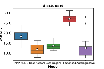
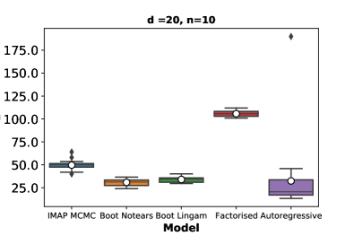
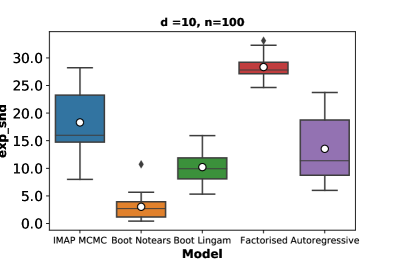
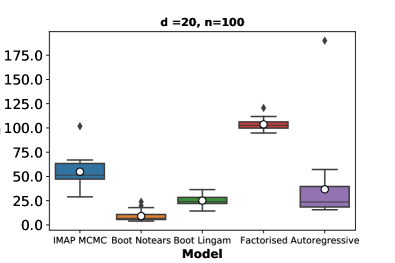
Figure 5: $\mathop{{}\mathbb{E}}\left[\text{SHD}\right]$ for $d=10$ and $d=20$ node ER random graphs (lower is better). Results obtained using 20 different random graphs.

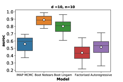
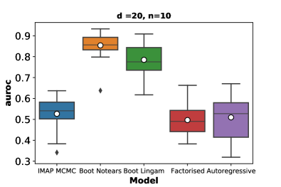
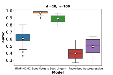
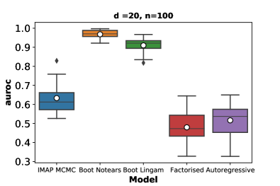
Figure 6: AUROC for $d=10$ and $d=20$ node ER random graphs (higher is better). Results obtained using 20 different random graphs.

4.2.3 Real Dataset

Table 1: Results on the Dream4 gene expression dataset in terms of AUROC.

	AUROC
IMAP MCMC	0.438 $\pm$ 0.02
Boot Notears	0.330
Boot Lingam	0.689
Factorised	0.489 $\pm$ 0.01
Autoregressive (VCN)	0.519 $\pm$ 0.03

We evaluate our method in terms of AUROC on edge feature probabilities against all the baselines on the Dream4 in-silico network challenge on gene regulation. As the typical metric for this challenge is the AUROC, we restrict our focus to this metric on this dataset. In particular, we examine the multifactorial dataset consisting of ten nodes and ten observations. Table 1 reports the AUROC of all the methods including the baselines. As the table suggests, our method achieves favourable performance while still being faster. In addition, we note that the underlying true graph corresponding to this dataset need not be a DAG, therefore introducing model misspacification.

5 Conclusion

We present a variational inference approach to perform Bayesian inference over the unknown causal structure in the structural causal model. Since the posterior over graph structures is multimodal in nature due to non-identifiability, we parameterise the variational family as an autoregressive distribution and model it using an LSTM. While we explore getting uncertainty estimates for linear models, it could be relevant to extend this to the case of non-linear models. One of the main limitations of this approach is the scalability of this method to larger dimensions. While a score function estimator might be limiting in higher dimensions due to higher variance, advanced variance reduction techniques could be used [11]. Further improvements to the proposed method can be obtained by combining with normalising flows for discrete variables [35, 18]. Nevertheless, the uncertainty estimates obtained in this framework can be useful for selecting the most informative interventions, performing budgeted interventional experiments as well as representation learning of high-dimensional signals like natural images [3].

Appendix A Proof of Proposition 1

Proof.

$$\begin{split}&\operatorname*{arg\,min}_{\phi}\operatorname{D_{KL}}{\left(q_{\phi}(\mathcal{G})||p(\mathcal{G}|{\mathcal{D}})\right)}\\ &\stackrel{{\scriptstyle Eq.\ref{eq:true_posterior}}}{{=}}\operatorname*{arg\,min}_{\phi}\mathop{{}\mathbb{E}}_{q_{\phi}(\mathcal{G})}[\log p({\mathcal{D}}|\mathcal{G})+\log p({\mathcal{D}})+\log q_{\phi}(\mathcal{G})-\log p(\mathcal{G})]\\[4.30554pt] &=\operatorname*{arg\,min}_{\phi}\mathop{{}\mathbb{E}}_{q_{\phi}(\mathcal{G})}\left[-\log p({\mathcal{D}}|\mathcal{G})\right]+\log p({\mathcal{D}})+\operatorname{D_{KL}}\left(q_{\phi}(\mathcal{G})||p(\mathcal{G})\right)\\[4.30554pt] \end{split}$$

which gives us a lower bound on the marginal log-likelihood of the data.

$$\begin{split}\log p({\mathcal{D}})\geq\mathop{{}\mathbb{E}}_{q_{\phi}(\mathcal{G})}\left[\log p({\mathcal{D}}|\mathcal{G})\right]-\operatorname{D_{KL}}\left(q_{\phi}(\mathcal{G})||p(\mathcal{G})\right)\\ \end{split}$$

∎

Appendix B Detailed Experimental Setup

B.1 Synthetic Data Generation

For generating synthetic data, we follow the procedure of NOTEARS [38]. We sample a DAG at random from an Erdos-Renyi model with expected number of edges equal to $d$. We only select the DAG if it has atleast two graphs inside the MEC. The edge weights are sampled independently at random from a Gaussian prior with a mean of $2$ and variance of $1$.The noise variables of the SCM are Gaussian mean 0 and variance of 1.

B.2 Experimental Details

Each model was then trained 20 times with different graphs (and hence datasets) for $n=10$ and $n=100$ data samples. For the plots of the true posterior comparison, we focus on $n=10$ samples. In addition, we also take the Hellinger distance instead of other divergences as the probabilities of many graph configurations are almost 0 and the log probabilities become numerically infeasible to tractably compute. For the factorised distribution and VCN, the models were trained with a learning rate of $1e-2$ with Adam optimiser [21] for 30k epochs where the Gibbs temperature of the DAG constraint $\lambda_{t}$ is annealed from 10 to 1000 with the following annealing schedule:

$$\lambda_{t}(i)=\text{min\_temp}+10^{\frac{-2\max(0,k-1.1i)}{k}}(\text{max\_temp}-\text{min\_temp})$$ (10)

where $k$ is the total number of epochs and $i$ is the current epoch. We set $\lambda_{s}$ to 0.01. We also note that $Z_{d}$ is the partition function of the Gibbs distribution which in practice cannot be computed easily for data with dimensionality $d\geq 5$. However, we note that computing this is not required for the optimisation of the ELBO (Eq. 7) as it turns out to be a constant.

B.3 BGe score

To compute the BGe score, the parameters $\theta$ have the following prior:

$$\begin{split}\bm{\theta}&\sim\mathcal{N}(\bm{\theta}|\mu,W^{-1})\\ p(\mu|\gamma,W,\alpha_{w})&=\mathcal{N}(\mu|\gamma,(\alpha_{\mu}W)^{-1})\\ p(W|\alpha_{\lambda},T)&:=\text{Wishart}(W|\alpha_{\lambda},T)\end{split}$$ (11)

We set $\gamma$ to 2, $\alpha_{\lambda}$ to 10 if $d\leq 5$ else we set it to 1000. $T$ is set to $\alpha_{\mu}\frac{\alpha_{\lambda}-d-1)}{\alpha_{\mu}+1}\cdot\mathbb{I}^{d\times d}$. The posterior for the above equation can be obtained with the same distribution family in close form and is given by:

$$\begin{split}p(\mu|W,{\mathcal{D}})&:=\mathcal{N}(\mu|\gamma^{\prime},W^{\prime})\\ \gamma^{\prime}&=\frac{\alpha_{\mu}\gamma+n\bar{x}_{n}}{\alpha_{\mu}+n}\\ W^{\prime}&=(\alpha_{\mu}+n)W\end{split}$$ (12)

$$\begin{split}p(W|{\mathcal{D}})&:=\text{Wishart}(\alpha_{w}^{\prime},T^{\prime})\\ \alpha_{w}^{\prime}&=\alpha_{w}+n\\ T^{\prime}&=T+S_{n}+\frac{\alpha_{\mu}n}{\alpha_{\mu}+n}(\gamma-\bar{x}_{n})(\gamma-\bar{x}_{n})^{T}\end{split}$$ (13)

where $\bar{x}_{n}=\sum_{i=1}^{n}x^{(i)}$ is the sample mean and $S_{n}=\sum_{i=1}^{n}(x^{(i)}-\bar{x}_{n})(x^{(i)}-\bar{x}_{n})^{T}$ is the sample covariance.

B.4 Baselines

Here we review the baselines which have been used for comparison and outline the hyperparameters and training procedures which have been used.

B.4.1 DAG Bootstrap

For the DAG bootstrap method, we ran Lingam [33] and NOTEARS [38] by resampling (with replacement) 50 points at random for 1000 different times for $n=100$ and 252 times with 5 points for $n=10$. An empirical estimate of the posterior $P(\mathcal{G}|\mathbf{x})=w_{\mathcal{G},\mathbf{x}}\mathbbm{1}(\mathcal{G}\in\mathcal{G}_{t})$ is obtained where $\mathcal{G}_{t}$ is the set of all graphs predicted during the Bootstrap procedure and $w_{\mathcal{G},\mathbf{x}}$ is the empirical normalised frequency count.

B.4.2 IMAP MCMC

We follow the default hyperparameters given in the IMAP MCMC paper [1]. In particular, we run the MCMC chain for $1e5$ iterations with a burn-in period of $2e4$ iterations. We use a thinning factor of 100 and use the same parameters for BGe score calculation as that for our approach.

B.4.3 Open Source Codes for Baselines

We use the following open source implementations for the baselines:

• NOTEARS: https://github.com/xunzheng/notears with Apache-2.0 License.

• Lingam: https://github.com/cdt15/lingam with MIT License.

• IMAP MCMC: https://github.com/miraep8/Minimal_IMAP_MCMC.

B.5 Real Dataset

For the Dream4 [32] gene-expression dataset, we use one of the gene expressions from the multifactorial dataset with ten nodes and ten observations. We also note that all the graphs in Dream4 do not necessarily correspond to DAGs, thereby introducing a crucial model misspacification in many of the models presented. We hypothesize that the inferior results of many of the techniques including the proposed approach suffer from this because of the non-DAGness.

References

- Agrawal et al. [2018] Raj Agrawal, Caroline Uhler, and Tamara Broderick. Minimal i-map mcmc for scalable structure discovery in causal dag models. In International Conference on Machine Learning, pages 89–98. PMLR, 2018.
- Agrawal et al. [2019] Raj Agrawal, Chandler Squires, Karren Yang, Karthik Shanmugam, and Caroline Uhler. Abcd-strategy: Budgeted experimental design for targeted causal structure discovery. arXiv preprint arXiv:1902.10347, 2019.
- Bengio et al. [2019] Yoshua Bengio, Tristan Deleu, Nasim Rahaman, Rosemary Ke, Sébastien Lachapelle, Olexa Bilaniuk, Anirudh Goyal, and Christopher Pal. A meta-transfer objective for learning to disentangle causal mechanisms. arXiv preprint arXiv:1901.10912, 2019.
- Blei et al. [2017] David M. Blei, Alp Kucukelbir, and Jon D. McAuliffe. Variational Inference: A Review for Statisticians. Journal of the American Statistical Association, 112(518):859–877, Apr 2017. ISSN 1537-274X. doi: 10.1080/01621459.2017.1285773. URL http://dx.doi.org/10.1080/01621459.2017.1285773.
- Bühlmann et al. [2014] Peter Bühlmann, Jonas Peters, Jan Ernest, et al. Cam: Causal additive models, high-dimensional order search and penalized regression. The Annals of Statistics, 2014.
- Chickering [2002] David Maxwell Chickering. Optimal structure identification with greedy search. Journal of machine learning research, 2002.
- Eberhardt and Scheines [2007] Frederick Eberhardt and Richard Scheines. Interventions and causal inference. Philosophy of science, 74(5):981–995, 2007.
- Ellis and Wong [2008] Byron Ellis and Wing Hung Wong. Learning causal bayesian network structures from experimental data. Journal of the American Statistical Association, 2008.
- Friedman and Koller [2003] Nir Friedman and Daphne Koller. Being bayesian about network structure. a bayesian approach to structure discovery in bayesian networks. Machine learning, 50(1):95–125, 2003.
- Geiger et al. [2002] Dan Geiger, David Heckerman, et al. Parameter priors for directed acyclic graphical models and the characterization of several probability distributions. The Annals of Statistics, 2002.
- Grathwohl et al. [2017] Will Grathwohl, Dami Choi, Yuhuai Wu, Geoffrey Roeder, and David Duvenaud. Backpropagation through the void: Optimizing control variates for black-box gradient estimation. arXiv preprint arXiv:1711.00123, 2017.
- Grzegorczyk and Husmeier [2008] Marco Grzegorczyk and Dirk Husmeier. Improving the structure mcmc sampler for bayesian networks by introducing a new edge reversal move. Machine Learning, 2008.
- Hauser and Bühlmann [2012] Alain Hauser and Peter Bühlmann. Characterization and greedy learning of interventional markov equivalence classes of directed acyclic graphs. Journal of Machine Learning Research, 2012. URL http://jmlr.org/papers/v13/hauser12a.html.
- Heckerman et al. [1999] David Heckerman, Christopher Meek, and Gregory Cooper. A bayesian approach to causal discovery. Computation, causation, and discovery, 1999.
- Heinze-Deml et al. [2018a] Christina Heinze-Deml, Marloes H Maathuis, and Nicolai Meinshausen. Causal structure learning. Annual Review of Statistics and Its Application, 5:371–391, 2018a.
- Heinze-Deml et al. [2018b] Christina Heinze-Deml, Jonas Peters, and Nicolai Meinshausen. Invariant causal prediction for nonlinear models. Journal of Causal Inference, 2018b.
- Hochreiter and Schmidhuber [1997] Sepp Hochreiter and Jürgen Schmidhuber. Long short-term memory. Neural computation, 1997.
- Hoogeboom et al. [2019] Emiel Hoogeboom, Jorn WT Peters, Rianne van den Berg, and Max Welling. Integer discrete flows and lossless compression. arXiv preprint arXiv:1905.07376, 2019.
- Ke et al. [2019] Nan Rosemary Ke, Olexa Bilaniuk, Anirudh Goyal, Stefan Bauer, Hugo Larochelle, Chris Pal, and Yoshua Bengio. Learning neural causal models from unknown interventions. arXiv preprint arXiv:1910.01075, 2019.
- Ke et al. [2020] Nan Rosemary Ke, Jane Wang, Jovana Mitrovic, Martin Szummer, Danilo J Rezende, et al. Amortized learning of neural causal representations. arXiv preprint arXiv:2008.09301, 2020.
- Kingma and Ba [2014] Diederik P Kingma and Jimmy Ba. Adam: A method for stochastic optimization. arXiv preprint arXiv:1412.6980, 2014.
- Kuipers and Moffa [2017] Jack Kuipers and Giusi Moffa. Partition mcmc for inference on acyclic digraphs. Journal of the American Statistical Association, 2017.
- Kuipers et al. [2014] Jack Kuipers, Giusi Moffa, David Heckerman, et al. Addendum on the scoring of gaussian directed acyclic graphical models. Annals of Statistics, 42(4):1689–1691, 2014.
- Lachapelle et al. [2019] Sébastien Lachapelle, Philippe Brouillard, Tristan Deleu, and Simon Lacoste-Julien. Gradient-based neural dag learning. arXiv preprint arXiv:1906.02226, 2019.
- Madigan et al. [1995] David Madigan, Jeremy York, and Denis Allard. Bayesian graphical models for discrete data. International Statistical Review/Revue Internationale de Statistique, 1995.
- Niinimäki et al. [2016] Teppo Niinimäki, Pekka Parviainen, and Mikko Koivisto. Structure discovery in bayesian networks by sampling partial orders. The Journal of Machine Learning Research, 2016.
- Pearl [2009] Judea Pearl. Causality. Cambridge university press, 2009.
- Peters et al. [2016] Jonas Peters, Peter Bühlmann, and Nicolai Meinshausen. Causal inference by using invariant prediction: identification and confidence intervals. Journal of the Royal Statistical Society: Series B (Statistical Methodology), 2016.
- Peters et al. [2017] Jonas Peters, Dominik Janzing, and Bernhard Schölkopf. Elements of causal inference. The MIT Press, 2017.
- Prill et al. [2010] Robert J Prill, Daniel Marbach, Julio Saez-Rodriguez, Peter K Sorger, Leonidas G Alexopoulos, Xiaowei Xue, Neil D Clarke, Gregoire Altan-Bonnet, and Gustavo Stolovitzky. Towards a rigorous assessment of systems biology models: the dream3 challenges. PloS one, 2010.
- Ramsey et al. [2017] Joseph Ramsey, Madelyn Glymour, Ruben Sanchez-Romero, and Clark Glymour. A million variables and more: the fast greedy equivalence search algorithm for learning high-dimensional graphical causal models, with an application to functional magnetic resonance images. International journal of data science and analytics, 2017.
- Schaffter et al. [2011] Thomas Schaffter, Daniel Marbach, and Dario Floreano. Genenetweaver: in silico benchmark generation and performance profiling of network inference methods. Bioinformatics, 2011.
- Shimizu [2014] Shohei Shimizu. LiNGAM: Non-Gaussian methods for estimating causal structures. Behaviormetrika, 2014.
- Spirtes et al. [2000] Peter Spirtes, Clark N Glymour, Richard Scheines, and David Heckerman. Causation, prediction, and search. MIT press, 2000.
- Tran et al. [2019] Dustin Tran, Keyon Vafa, Kumar Agrawal, Laurent Dinh, and Ben Poole. Discrete flows: Invertible generative models of discrete data. In Advances in Neural Information Processing Systems, 2019.
- Williams [1992] Ronald J Williams. Simple statistical gradient-following algorithms for connectionist reinforcement learning. Machine learning, 1992.
- Yu et al. [2019] Yue Yu, Jie Chen, Tian Gao, and Mo Yu. Dag-gnn: Dag structure learning with graph neural networks. arXiv preprint arXiv:1904.10098, 2019.
- Zheng et al. [2018] Xun Zheng, Bryon Aragam, Pradeep K Ravikumar, and Eric P Xing. Dags with no tears: Continuous optimization for structure learning. In Advances in Neural Information Processing Systems, pages 9472–9483, 2018.