Nonperturbative renormalization of the quark chromoelectric dipole moment with the gradient Flow: Power divergences

Abstract

The $CP$-violating quark chromoelectric dipole moment (qCEDM) operator, contributing to the electric dipole moment (EDM), mixes under renormalization and particularly on the lattice with the pseudoscalar density. The mixing coefficient is power-divergent with the inverse lattice spacing squared, $1/a^{2}$, regardless of the lattice action used. We use the gradient flow to define a multiplicatively renormalized qCEDM operator and study its behavior at small flow time. We determine nonperturbatively the linearly divergent coefficient with the flow time, $1/t$, up to subleading logarithmic corrections, and compare it with the 1-loop perturbative expansion in the bare and renormalized strong coupling. We also discuss the O($a$) improvement of the qCEDM defined at positive flow time.

I Introduction

The Standard Model (SM) of particle physics is described by a Lagrangian density of dimension $d=4$, with fundamental fields associated with all the elementary particles already experimentally observed. Physics beyond the Standard Model (BSM) at the hadronic scale can be described by higher dimensional ($d>4$) operators, with coefficients usually suppressed, up to logarithmic corrections, by powers of the BSM energy scale $1/\Lambda_{\textrm{BSM}}^{d-4}$.

The baryon asymmetry in the universe can be determined by comparing the abundances of the light elements (D, ³He, ⁴He) determined experimentally with the prediction of standard big-bang nucleosynthesis [1, 2]. A completely independent determination of the baryon asymmetry can be obtained from the cosmic microwave background (CMB) [3, 4] giving perfectly consistent results [5]. The amount of $CP$-violation stemming from the CKM (Cabibbo-Kobayashi-Maskawa) matrix [6, 7, 8] is impossible to reconcile with the amount of $CP$-violation needed to explain the observed baryon asymmetry. This lead to the conclusion that new sources of $CP$-violation are needed.

$CP$-violation can be investigated by studying the electric dipole moment (EDM) of particles with nonzero spin. The current bound on the neutron EDM (nEDM) [9] is several orders of magnitude larger than the value of the nEDM that would be induced by the CKM matrix in the weak sector [10]. An experimental signal of a nonzero EDM would thus provide strong evidence for BSM physics.

To provide possible clues on the type of BSM physics it is crucial to determine separately every $CP$-violating contribution to a nonzero EDM. Using lattice QCD it is possible, at least in principle, to determine the renormalized matrix elements of the $CP$-violating operators. An important contribution to the EDM comes from the $CP$-violating chromoelectric quark operator

$$O_{\textrm{C}}^{ij}(x)=\overline{\psi}_{i}(x)\gamma_{5}\sigma_{\mu\nu}F_{\mu\nu}(x)\psi_{j}(x)\,,$$ (1)

where $\psi_{i}$ and $\overline{\psi}_{i}$ are fermion fields with flavor $i=1,\ldots,N_{f}$, and $F_{\mu\nu}(x)=F_{\mu\nu}^{a}(x)T^{a}$ is the gluon field tensor with $a=1,\ldots,8$. The operator is known as the quark chromoelectric dipole moment (qCEDM) operator.

The determination of the renormalized qCEDM using lattice QCD is particularly difficult because the $O_{\textrm{C}}$ operator mixes under renormalization with the lower-dimensional pseudoscalar density and this poses a challenge in extracting the physical matrix element. In this paper we advocate the use of the gradient flow [11, 12, 13, 14] to define the quark chromo-EDM.

The qCEDM defined at nonvanishing flow time, $t$, is multiplicatively renormalizable and to determine the physical matrix element one needs to study its behavior at small flow time. The local operators contributing to the short flow time expansion have the same symmetry transformation properties of the qCEDM. Of particular importance is the leading behavior at small flow time stemming from the pseudoscalar density, which scales as $1/t$ and is thus linearly divergent with the flow time.

Power divergences have been tackled in several ways, for example by imposing renormalization conditions on hadronic matrix elements at finite lattice spacing (see e.g. [15]). We use the gradient flow to probe the short distance behavior of the quark chromoelectric dipole moment and determine nonperturbatively the mixing coefficient of the qCEDM operator with the lowest dimensional operator – in this case the pseudoscalar density.

Here the application of the gradient flow is potentially advantageous for several reasons. We can perform the continuum limit at each stage of the calculation at finite flow time $t$, thus the classification of the operators contributing to the renormalization of the qCEDM can be done using continuum symmetries. Additionally the analysis of cutoff effects is simplified [13] and, by using chiral symmetry transformation at finite flow time [16], we can determine the leading dimension $6$ operators contributing to the O($a$) cutoff effects.

If the lattice QCD action breaks chiral symmetry, the qCEDM mixes with lower dimensional operators with different chiral transformation properties, such as the topological charge density. The definition of the qCEDM at nonzero flow time allows us to perform the continuum limit at fixed flow time, thus forbidding the contribution of such operators to the small flow time behavior. The taming of induced power divergences at finite flow time $t$ is the main advantage of the gradient flow and thus motivates our use of it with regards to the $O_{\textrm{C}}$ operator.

In this paper we determine the linearly divergent mixing coefficient of the qCEDM with the pseudoscalar density as function of the renormalized and bare strong coupling. We note that the particular dependence on the bare coupling is specific to the lattice action chosen in this paper, which is the Iwasaki gauge action [17] with O($a$) improved Wilson fermions [18, 19, 20].

The paper is organized as follows: we introduce the main definitions and discuss the power divergences in the context of flowed fields in Sec. II. In Sec. III we define the lattice correlation functions we analyze and discuss the O($a$) improvement of the qCEDM at finite flow time $t$. Our analysis and the ensuing results are presented in Sec. IV in terms of the renormalized coupling and in Sec. IV.2 in terms of the bare coupling. In Sec. V we show results for the specific O($a$) contributions to the flowed correlation functions. We finally recapitulate our findings and provide an outlook on future calculations in Sec. VI. We defer to Appendices A and B for more details of our numerical analysis and in Appendix C we discuss the perturbative calculation performed using the same scheme adopted in this paper for the nonperturbative determination of the mixing with the pseudoscalar density.

II Quark chromoelectric dipole moment at short flow time

In this section we discuss the definition of the qCEDM with flowed fermion and gauge fields, its behavior at small flow time $t$ and the definition of the lattice correlation functions. We assume that the reader is familiar with the gradient flow (GF) formalism for both for gauge and fermion fields [11, 12, 14]. Otherwise, for detailed references on the gradient flow and the use of the gradient flow to determine $CP$-violating operators contributing to the EDM we recommend the reader to consult [16, 21, 22, 23, 24, 25, 26, 27], and the recent review [28]. Our numerical implementation of the GF for fermions using a 4th-order Runge-Kutta integration scheme follows closely that of [11].

We denote the fermion and antifermion fields with flavor $i$ at nonzero flow time $t$ as $\chi_{i}(x;t)$, and $\overline{\chi}_{i}(x;t)$, respectively, and the gluon fields $B_{\mu}(x;t)$. We define the qCEDM operator at nonzero flow time as

$$O_{\textrm{C}}^{ij}(x;t)=\overline{\chi}_{i}(x;t)\gamma_{5}\sigma_{\mu\nu}G_{\mu\nu}(x;t)\chi_{j}(x;t)\,,$$ (2)

where $\sigma_{\mu\nu}=\frac{i}{2}\left[\gamma_{\mu},\gamma_{\nu}\right]$ and $G_{\mu\nu}(x;t)$ is the gauge field tensor with flowed field $B_{\mu}(x;t)$.

At vanishing flow time, $t=0$, the renormalization of the qCEDM is nontrivial, and it mixes divergently with several operators of the same dimension and less, $d\leq 5$. The list of operators that can mix with the qCEDM has been analyzed in Ref. [29] in the context of the RI-MOM renormalization of the qCEDM and classified based on their engineering dimension. The proliferation of local operators contributing to the mixing motivates in large measure our use of the gradient flow to define the nonperturbatively renormalized qCEDM operator. We note that in Ref. [30] the qCEDM has been renormalized in the $\overline{\rm MS}$ scheme using a background gauge to ensure that only gauge invariant divergences contribute. Our method, described below in Sec. II.1, is based on the short flow time expansion [14] and, as it will become clear in the next section, is based on gauge invariant correlation functions.

Taking into account gauge invariance the list of operators reduces to

$$P^{ij},\quad\partial^{2}P^{ij},\quad\frac{e(q_{i}+q_{j})}{2}\overline{\psi}_{i}\gamma_{5}\sigma_{\mu\nu}F_{\mu\nu}^{\textrm{em}}\psi_{j}\,,$$ (3)

where $F_{\mu\nu}^{\textrm{em}}$ is the electromagnetic field tensor and $q_{i}$ is the quark $i$ charge in units of the proton charge. Other operators, proportional to the quark mass, can contribute at small flow time, but we choose a massless scheme and our results are extrapolated to zero quark mass.

In this work we focus only on the power divergence of the qCEDM and the only contribution to the power divergence comes from the pseudoscalar density

$$P^{ij}(x)=\overline{\psi}_{i}(x)\gamma_{5}\psi_{j}(x)\,.$$ (4)

If we perform our renormalization using the lattice as a regulator, the mixing pattern will depend on the choice of the lattice action and in particular whether the action preserves (a remnant of) chiral symmetry or not.

The renormalization of the qCEDM presented in Ref. [29] assumes that the lattice action breaks chiral symmetry, thus the classification of operators includes the ones with opposite chirality with respect to the qCEDM, such as the topological charge density. For example, if our calculation were to use the RI-MOM scheme and nonperturbatively O($a$) improved Wilson fermions [18, 20], operators of dimension $d=4$, with opposite chirality with respect to the qCEDM operator, would contribute to a linear power divergence in the lattice spacing, $\sim 1/a$. These additional operators have been also classified in Ref. [29].

As our strategy to study the power divergences is based on the use of the GF, we can perform the continuum limit before studying the short distance behavior of the qCEDM. This allows to classify operators using the symmetries of the continuum theory, such as chiral symmetry.

Operators with opposite chirality do contribute to O($a$) cutoff effects of the qCEDM correlation functions under the GF, however. Such contributions can be analyzed using a Symanzik effective theory at finite flow time [13] and then using a generalization of chiral symmetry at finite flow time [16]. We present our analysis of this effect relevant for the qCEDM in Sec. V.

II.1 Short flow time expansion

To study the power divergent mixing of the qCEDM operator with the pseudoscalar density $P^{ij}$, we probe the short distance behavior of the qCEDM with the GF and by means of the short flow time expansion (SFTE). The SFTE, as the name suggests, is an operator product expansion for $t\rightarrow 0$. Its application is valid for renormalized fields and can be used to define renormalized operators via nonperturbative subtraction at nonvanishing flow time [14]. We first perform the SFTE in the continuum assuming that any correlation function calculated on a lattice with spacing $a$ has been extrapolated to the continuum at a fixed physical value of the flow time $t$. We do not specify at the moment the renormalization scheme we use to renormalize the operators. The SFTE reads

$$\left[O_{\textrm{C}}^{ij}\right]_{R}(x;t)\stackrel{{\scriptstyle t\rightarrow 0}}{{\sim}}c_{\textrm{CP}}(t)P_{R}^{ij}(x)\,,$$ (5)

where $c_{\textrm{CP}}\sim 1/t$ and we have neglected any additional contribution coming from higher dimensional operators. The final goal is to determine nonperturbatively the coefficient $c_{\textrm{CP}}$ so as to subtract the power divergence and thus renormalize our qCEDM matrix element of interest.

The expansion coefficient $c_{\textrm{CP}}=c_{\textrm{CP}}^{(1)}g^{2}+O(g^{4})$ can be also computed in perturbation theory and its value can provide us with the behavior of $c_{\textrm{CP}}$ at small coupling. In Ref. [23] we have calculated $c_{\textrm{CP}}$ at one-loop order in perturbation theory in an off-shell scheme with two external quarks obtaining

$$c_{\textrm{CP}}=c_{\textrm{CP}}^{(1)}\overline{g}^{2}+O(\overline{g}^{4})\,,\qquad c_{CP}^{(1)}=\frac{1}{2\pi^{2}t}\,,$$ (6)

where $\overline{g}$ denotes the strong coupling renormalized at a scale $\mu=(8t)^{-1/2}$. We have repeated the perturbative calculation of $c_{\textrm{CP}}$, using the same gauge invariant correlation functions that we use in our nonperturbative lattice determination of $c_{\textrm{CP}}$ described in Secs. (II.2, IV, IV.2). Details on the perturbative calculation can be found in Appendix C. The final result for the linear divergence is the same as the one obtained in Ref. [23] given by Eq. (6). This result suggests a form of universality for the leading order divergence. We comment in more details on this result in Appendix C.

II.2 Lattice correlators

We have a certain amount of freedom when choosing how to compute the expansion coefficient nonperturbatively of a given correlator. Being an operator relation, the SFTE can be applied to different correlation functions, the choice of which is only dictated by theoretical or numerical convenience. The specific choice of the external state allows one to select, to a certain extent, which operators that contribute to the SFTE we want to study. We use gauge invariant correlation functions that are numerically unproblematic and allows us to select the contribution coming from the pseudoscalar density to the SFTE shown in Eq. (5).

We consider a four-dimensional, hypercubic Euclidean lattice with spacing $a$ and we define the two-point function

$$\Gamma_{CP}(x_{4};t)=a^{3}\sum_{{\bf x}}\left\langle O_{\textrm{C}}^{ij}(x_{4},{\bf x};t)P^{ji}(0,{\bf 0};0)\right\rangle\,,\qquad$$ (7)

where the probe is represented by the pseudoscalar density at $t=0$. To define the lattice correlation function we need to specify the form of the field tensor

$$G_{\mu\nu}(x)=\frac{1}{8ia^{2}}\left[Q_{\mu\nu}(x)-Q_{\nu\mu}(x)\right]\,,$$ (8)

where $Q_{\mu\nu}(x)$ is the “clover” term, i.e. the sum of the $4$ plaquettes in the $\mu\nu$ plane around the point $x$.

Inserting the SFTE (5) in Eq. (7) and thereby neglecting higher dimensional operators, we obtain

$$\left[\Gamma_{CP}(x_{4};t)\right]_{R}=c_{\textrm{CP}}\left[\Gamma_{PP}(x_{4})\right]_{R}\,,$$ (9)

where

$$\Gamma_{PP}(x_{4})=\Gamma_{PP}(x_{4};t=0)=a^{3}\sum_{{\bf x}}\left\langle P^{ij}(x_{4},{\bf x};t=0)P^{ji}(0,{\bf 0})\right\rangle\,,$$ (10)

is the usual pseudoscalar two-point function. The SFTE suggests that the following dimensionless renormalized ratio

$$\left[R_{P}(x_{4};t)\right]_{R}=t\frac{\left[\Gamma_{CP}(x_{4};t)\right]_{R}}{\left[\Gamma_{PP}(x_{4})\right]_{R}}\,,$$ (11)

tends to $t\cdot c_{\textrm{CP}}$ for small enough values of $t$. Before detailing the method, we want to comment on this particular choice to determine $c_{\textrm{CP}}$. We could have chosen any interpolator with the quantum numbers of the qCEDM, but we find the pseudoscalar density very convenient to work with. Another important aspect is the choice to keep $O_{\textrm{C}}$ and $P$ at nonzero physical distance $x_{4}>0$. This choice is done to avoid possible spurious contact terms at $x_{4}\sim 0$. We also notice that the denominator of $R_{P}$ will have additional contact terms if $x_{4}=0$.

In determining $c_{\textrm{CP}}$ it is advantageous to study the correlation functions in Eq. (11) for large Euclidean times $x_{4}\gg\sqrt{8t}$. Performing a spectral decomposition of the $2$ correlation functions (7) and (10) and retaining only the contributions of the ground state we obtain

$$\Gamma_{CP}(x_{4};t)=\frac{1}{2m_{\pi}}\left\langle 0|O_{\textrm{C}}^{ij}(t)|\pi\right\rangle\left\langle\pi|P^{ij}|0\right\rangle{\rm{e}}^{-m_{\pi}x_{4}}\,,$$ (12)

$$\Gamma_{PP}(x_{4})=\frac{1}{2m_{\pi}}\left\langle 0|P^{ij}|\pi\right\rangle\left\langle\pi|P^{ij}|0\right\rangle{\rm{e}}^{-m_{\pi}x_{4}}\,,$$ (13)

where $\left.|\pi\right\rangle$ is the pion state. The bare ratio $R_{P}$ thus has a spectral decomposition for large $x_{4}$

$$R_{P}(t)=t\frac{\left\langle 0|\left[O_{\textrm{C}}\right]_{R}^{ij}(t)|\pi\right\rangle}{\left\langle 0|P_{R}^{ij}|\pi\right\rangle}\,.$$ (14)

The renormalization of the pseudoscalar density and any flowed operators is well understood [11, 12, 13]

$$P_{R}^{ij}=Z_{P}P^{ij}\,,\qquad\left[O_{\textrm{C}}\right]_{R}^{ij}(t)=Z_{\chi}O_{\textrm{C}}^{ij}(t)\,,$$ (15)

where $Z_{\chi}^{1/2}$ is the renormalization factor of the flowed fermion field. If we make explicit the renormalization constants in Eq. (9) we then obtain

$$Z_{\chi}\Gamma_{CP}(x_{4};t)=c_{\textrm{CP}}Z_{P}\Gamma_{PP}(x_{4})\,.$$ (16)

To determine $c_{\textrm{CP}}$ in the continuum limit we need an independent determination of $Z_{P}$ and $Z_{\chi}$ (or the use of the ringed fermion fields [25]). In this first study of the qCEDM we calculate $2$ different quantities. The first is the nonperturbative renormalization that connects the qCEDM at finite flow time with the pseudoscalar density, also at finite flow time. This quantity, labeled $\Delta(\overline{g}^{2})$ below in Eq. (21), is finite and represents the leading dependence of the coefficient of the linear divergence on the renormalized coupling. The second quantity we calculate is the bare expansion coefficient of the linear divergence divided by $Z_{\chi}$, labeled $c_{\chi}$ below in Eq. (23).

To calculate the finite renormalization, instead of using the ratio $R_{P}(x_{4};t)$ in Eq. (11), we consider the ratio

$$\left[\overline{R}_{P}(x_{4};t)\right]_{R}=t\frac{\left[\Gamma_{CP}(x_{4};t)\right]_{R}}{\left[\Gamma_{PP}(x_{4};t)\right]_{R}}\,,$$ (17)

where the denominator now contains a flowed pseudoscalar density

$$\Gamma_{PP}(x_{4};t)=a^{3}\sum_{{\bf x}}\left\langle P^{ij}(x_{4},{\bf x};t)P^{ji}(0,{\bf 0})\right\rangle\,,$$ (18)

where

$$P^{ij}(x;t)=\overline{\chi}_{i}(x;t)\gamma_{5}\chi_{j}(x;t)\,.$$ (19)

The reason for this definition is that now we can perform the continuum limit of $\overline{R}_{P}(x_{4};t)$ without any knowledge of renormalization factors since the ratio in Eq. (17) is scheme independent and free of renormalization ambiguities. To determine the expansion coefficient $c_{\textrm{CP}}$ one still needs to determine the expansion coefficient, $c_{\textrm{P}}$, of the pseudoscalar density, $P^{ij}(x;t)$

$$P^{ij}(x;t)=c_{\textrm{P}}(t)P^{ij}(x)+{\mathcal{O}}(t)\,.$$ (20)

We do this via the relation

$$c_{\textrm{CP}}(t)=\frac{1}{t}\Delta(\overline{g}^{2})c_{\textrm{P}}(t)+{\mathcal{O}}(t)\,,$$ (21)

where $\Delta(\overline{g}^{2})$ is the nonperturbative finite renormalization we determine in this work:

$$\Delta(\overline{g}^{2})=\left[\overline{R}_{P}(x_{4};t)\right]_{R}\,,\qquad x_{4}\gg\sqrt{8t}\,.$$ (22)

In this way we determine nonperturbatively the power-divergent coefficient up to subleading logarithmic corrections described by of the expansion coefficient of the pseudoscalar density. Using the gradient flow shows that we can determine the power-divergent coefficient in the continuum limit, and once we determine the expansion coefficient $c_{\textrm{P}}$ of the pseudoscalar density it is possible to estimate also the subleading logarithmic contribution to the power divergence. Operating with the RG operator $\mu\frac{d}{d\mu}$ on the SFTE of the pseudoscalar density (20), it is possible to determine the flow time dependence of the expansion coefficient $c_{\textrm{P}}$ given the anomalous dimension of the pseudoscalar density, of the flowed fermion field and the beta function [14]. We leave the determination of $c_{\textrm{P}}$ for a future work.

The second quantity we determine is the bare expansion coefficient

$$c_{\chi}\equiv\frac{t}{Z_{\chi}}c_{\textrm{CP}}=\frac{1}{Z_{P}}R_{P}(x_{4};t)\,,$$ (23)

and make use of the determination of $Z_{P}(g_{0}^{2})$ in Ref. [31] (the values of $Z_{P}$ are also listed for completeness in Table 1). With this definition we can study the dependence of $c_{\chi}$ on the bare coupling $g_{0}$ leaving for future calculations the determination of $Z_{\chi}$ or the use of ”ringed” fermion fields [25]. Employing a Padé approximant in combination with perturbation theory, we determine the dependence on the bare coupling of $c_{\chi}$ for our choice of the lattice action. In Sec. IV we present the numerical details for the determination of $\Delta(\overline{g}^{2})$, while in Sec. IV.2 we show results for $c_{\chi}$.

III O($a$) improvement of the Quark Chromoelectric Dipole Moment operator

The theoretical analysis of cutoff effects in lattice field theory follows the Symanzik description [32, 33, 19, 20] in terms of effective action and operators close to the continuum limit. To study the cutoff effects of correlation functions involving fields at positive flow time $t$, it is better to rely on the quantum theoretical description based on the $4+1$ dimensional field theory [13, 16, 34]. The extra dimension is represented by the flow time $t$ and the GF equations are imposed augmenting the theory with an additional Grassmanian field $\lambda$ that acts as a Lagrange multiplier. With this field theoretical description it is possible to write the corresponding Symanzik effective action by adding higher dimensional operators to the continuum theory. We recall that the higher dimensional operators are constrained by the symmetries of the lattice theory.

We consider here nonperturbatively clover-improved Wilson fermions and gauge invariant correlation functions of fields, at nonzero physical distance with each other. With this prescription we can use the equations of motion to reduce the number of higher dimensional operators and thus avoid spurious O($a$) terms stemming from contact terms.

Following Ref. [13] the lattice action is improved by adding the following $d=5$ operators

$${\mathcal{O}}_{1}(x)=\frac{i}{4}\sum_{i=1}^{N_{f}}\overline{\psi}_{i}(x)\sigma_{\mu\nu}F_{\mu\nu}(x)\psi_{i}(x)\,,$$ (24)

$${\mathcal{O}}_{2}(x)=\sum_{i=1}^{N_{f}}\overline{\lambda}_{i}(x)\lambda_{i}(x)\,,$$ (25)

where $\lambda(x)$ is the Lagrange multiplier that, once integrated over in the Functional Integral, enforces the fermion fields, defined at positive flow time, to be solutions of the GF equations. We discuss in Appendix A how we numerically contract the Lagrange multiplier with the fermion fields. Here we just recall the basic properties. The field $\lambda$ has energy dimension $\frac{5}{2}$ in $d=4$ spacetime dimensions and the chiral transformation properties of this field are described in Ref. [16], as well as those of other higher dimensional operators. The operator ${\mathcal{O}}_{2}$ breaks chiral symmetry and is present as an O($a$) operator in the Symanzik effective action. The O($a$) operators are all evaluated at $t=0$, i.e. they are boundary terms for the $4+1$ dimensional theory. This is a consequence of the invariance of the action under chiral symmetry in the bulk of the $4+1$ dimensional theory [16]. While the term proportional to ${\mathcal{O}}_{1}$ is the usual clover term, with a tunable ${\textrm{c}}_{\textrm{sw}}$ parameter in the lattice action, the term proportional to ${\mathcal{O}}_{2}$ has a tunable $c_{\textrm{fl}}$ coefficient that only contributes to contractions between fermion fields at nonvanishing flow time [13]. In this work we will never consider fermion contractions between two flowed fermion fields, thus from now on we assume that $c_{\textrm{fl}}$ is not needed to remove O($a$) effects from the lattice correlators we compute.

The effective action is not sufficient to describe correlation functions in the Symanzik effective theory. We also need to consider O($a$) terms from the local operators. The list of higher dimensional operators, parametrizing O($a$) cutoff effects, for the fermion fields and the pseudoscalar and scalar densities is given in Ref. [13]. Here we just list for completeness the form of the renormalized O($a$) improved operators using the same notation as in [13]. For the fields at positive flow time the renormalization is dictated always by the same field renormalization factor $Z_{\chi}^{1/2}$. Chiral symmetry implies that only O($am$) contributions be present,

$$\chi_{R}(x,t)=Z_{\chi}^{1/2}\left(1+a~{}\frac{b_{\chi}}{2}m_{q}+a~{}\frac{\overline{b}_{\chi}}{2}{\rm{Tr}}M\right)\chi(x,t)\,,$$ (26)

$$P^{ij}_{R}(x,t)=Z_{\chi}\left(1+a~{}b_{\chi}m_{q,ij}+a~{}\overline{b}_{\chi}{\rm{Tr}}M\right)P^{ij}(x,t)\,,$$ (27)

where $m_{q}$ is the subtracted bare quark mass and $m_{q,ij}$ is the average of the subtracted quark masses, $m_{q,ij}=\frac{1}{2}(m_{q,i}+m_{q,j})$. To determine the subtracted quark mass it is possible to use the PCAC mass,

$$m_{q,ij}=\frac{\sum_{\bf x}\left\langle\partial_{0}A_{0}^{ij}(x_{4},{\bf x};0)P^{ji}(0;0)\right\rangle}{\sum_{\bf x}\left\langle P^{ij}(x_{4},{\bf x};0)P^{ji}(0;0)\right\rangle}\,.$$ (28)

The correlator on the right-hand-side (rhs) of Eq. (28) should be independent of $x_{4}$ up to cutoff effects.

With respect to the standard treatment of O($a$) cutoff effects, the fields at the boundary $t=0$ show additional O($a$) terms, if these are then contracted with fields at positive flow time

$$\left[A_{\mu}^{ij}(x)\right]_{I}=A_{\mu}^{ij}(x)+a~{}c_{A}\partial_{\mu}P^{ij}(x)+a~{}\widetilde{c}_{A}\widetilde{A}_{\mu}^{ij}(x)\,,$$ (29)

$$\left[P^{ij}(x)\right]_{I}=P^{ij}(x)+a~{}\widetilde{c}_{P}\widetilde{P}^{ij}(x)\,.$$ (30)

The two additional O($a$) terms are proportional to

$$\widetilde{A}_{\mu}^{ij}(x)=\overline{\lambda}_{i}(x)\gamma_{\mu}\gamma_{5}\psi_{j}(x)+\overline{\psi}_{i}(x)\gamma_{\mu}\gamma_{5}\lambda_{j}(x)\,,$$ (31)

$$\widetilde{P}^{ij}(x)=\overline{\lambda}_{i}(x)\gamma_{\mu}\gamma_{5}\psi_{j}(x)+\overline{\psi}_{i}(x)\gamma_{\mu}\gamma_{5}\lambda_{j}(x)\,.$$ (32)

The presence of the Lagrange multipliers confirms that these O($a$) terms contribute only when contracted with flowed local operators. According to Ref. [13] at tree level perturbation theory we have

$$c_{\textrm{fl}}=-\widetilde{c}_{A}=-\widetilde{c}_{P}=\frac{1}{2}\,,\qquad b_{\chi}=1\,.$$ (33)

To determine the O($a$) terms for the qCEDM operator we consider its chiral symmetry properties and construct the higher dimensional operator following Ref. [16]. Any operator of the form $\overline{\chi}_{i}(t)\Gamma(t)\chi_{j}(t)$ at $t>0$, where $\Gamma(t)$ is either constant or it contains, as in this case, the flowed gauge field, renormalizes with $Z_{\chi}$ and shows only O($am$) cutoff effects

$$\left[O_{\textrm{C}}^{ij}(x,t)\right]_{R}=Z_{\chi}\left[O_{\textrm{C}}^{ij}(x,t)\right]_{I}\,,\qquad\left[O_{\textrm{C}}^{ij}(x,t)\right]_{I}=\left(1+a~{}b_{\chi}m_{q,ij}+a~{}\overline{b}_{\chi}{\rm{Tr}}M\right)O_{\textrm{C}}^{ij}(x,t)\,,$$ (34)

where again this form is constrained by the chiral symmetry at $t>0$. In addition to the O($a$) terms shown in (34), we have to add an additional O($a$) improvement term because the pseudoscalar density is contracted with a field at nonvanishing flow time, which introduces the term proportional to $\widetilde{P}^{ij}$. The final form of the renormalized and improved correlation function is then

$$\left[\Gamma_{CP}(x_{4};t)\right]_{R}=Z_{\chi}Z_{P}\left[\Gamma_{CP}(x_{4};t)\right]_{I}\,,$$ (35)

$$\left[\Gamma_{CP}(x_{4};t)\right]_{I}=\left(1+a~{}b_{\chi}m_{q,ij}+a~{}\overline{b}_{\chi}{\rm{Tr}}M\right)\Gamma_{CP}(x_{4};t)+a~{}\widetilde{c}_{P}\widetilde{\Gamma}_{CP}(x_{4};t)\,,$$ (36)

where

$$\widetilde{\Gamma}_{CP}(x_{4};t)=a^{3}\sum_{{\bf x}}\left\langle O_{\textrm{C}}^{ij}(x_{4},{\bf x};t)\widetilde{P}^{ji}(0,{\bf 0};0)\right\rangle\,.$$ (37)

To improve the denominator in the ratio of Eq. (17) we define

$$\left[\Gamma_{PP}(x_{4};t)\right]_{R}=Z_{\chi}Z_{P}\left[\Gamma_{PP}(x_{4};t)\right]_{I}\,,$$ (38)

$$\left[\Gamma_{PP}(x_{4};t)\right]_{I}=\left(1+a~{}b_{\chi}m_{q,ij}+a~{}\overline{b}_{\chi}{\rm{Tr}}M\right)\Gamma_{PP}(x_{4};t)+a~{}\widetilde{c}_{P}\widetilde{\Gamma}_{PP}(x_{4};t)\,,$$ (39)

where

$$\widetilde{\Gamma}_{PP}(x_{4};t)=a^{3}\sum_{{\bf x}}\left\langle P^{ij}(x_{4},{\bf x};t)\widetilde{P}^{ji}(0,{\bf 0};0)\right\rangle\,.$$ (40)

The renormalized and improved ratio $\overline{R}_{P}$ then reads

$$\left[\overline{R}_{P}(x_{4};t)\right]_{R}=t\frac{\left[\Gamma_{CP}(x_{4};t)\right]_{I}}{\left[\Gamma_{PP}(x_{4};t)\right]_{I}}\,.$$ (41)

We show in Sec. IV.2 (see Figs. 12,13) that the O($a$) terms proportional to $\widetilde{\Gamma}_{CP}(x_{4};t)$ and $\widetilde{\Gamma}_{PP}(x_{4};t)$ vanish for $x_{4}$ slightly larger than zero for any value of the flow time we consider.

To improve the ratio in Eq. (11) we also need to improve the denominator

$$\left[\Gamma_{PP}(x_{4})\right]_{I}=\left(1+a~{}b_{P}m_{q,ij}+a~{}\overline{b}_{P}{\rm{Tr}}M\right)\Gamma_{PP}(x_{4})\,,$$ (42)

where the tree-level value is $b_{p}^{(0)}=1$. All the coefficients coming from sea quark effects on fermion correlation functions, such as the parameters $\overline{b}_{X}=O(g^{4})$, are neglected. The tree level value of $b_{P}$ coincides with the value of $b_{\chi}$ thereby simplifying the ratio (11). Thus we are left with O($am$) discretization errors of O($g^{2}$). The O($am$) terms of the pseudoscalar density probing the qCEDM in Eqs. (36, 42) simplify once we determine the ratios in Eqs. (11, 17).

In the next section we evaluate the correlation functions in Eqs. (37, 40) and show that it contributes only at short distances when $x_{4}\sim\sqrt{8t}$. To conclude, at nonzero physical distances $x_{4}\gg\sqrt{8t}$, for all practical purposes the ratio in Eq. (17) is renormalization group invariant and automatically O($a$) improved, after we improve the action, while the ratio in Eq. (11) is O($a$) improved, up to O($amg^{2}$).

IV Numerical Analysis

Table 1: Summary of the lattice bare parameters for the ensembles used. $N_{G}$ is the number of gauge configurations and $Z_{P}$ is the value of the renormalization constant determined in Ref. [31].

Designation	$\beta$	$\kappa_{l}$	$\kappa_{s}$	L/a	T/a	${\textrm{c}}_{\textrm{sw}}$	$N_{G}$	$a$ [fm]	$m_{\pi}$ [MeV]	$m_{N}$ [GeV]	$Z_{P}$
M1	1.90	0.13700	0.1364	32	64	1.715	399	0.0907(13)	699.0(3)	1.585(2)	0.49605
M2	1.90	0.13727	0.1364	32	64	1.715	400	0.0907(13)	567.6(3)	1.415(3)	0.49605
M3	1.90	0.13754	0.1364	32	64	1.715	450	0.0907(13)	409.7(7)	1.219(4)	0.49605
A1	1.83	0.13825	0.1371	16	32	1.761	800	0.1095(25)	710(1)	1.65(1)	0.44601
A2	1.90	0.13700	0.1364	20	40	1.715	790	0.0936(33)	676.3(7)	1.549(6)	0.49605
A3	2.05	0.13560	0.1351	28	56	1.628	650	0.0684(41)	660.4(7)	1.492(5)	0.51155

To determine the ratios $R_{P}$ and $\overline{R}_{P}$ in Eqs. (11, 17) we need to calculate the two-point functions in Eqs. (7, 10) and (18). We use publicly available [35] lattice gauge configurations generated with the Iwasaki gauge action [17] and nonperturbatively clover-improved fermions [18, 20]. Details on the generation of these ensembles can be found in Refs. [36, 31]. The improvement coefficient ${\textrm{c}}_{\textrm{sw}}$ for this choice of lattice action has been determined in Ref. [37]. The bare parameters of our ensembles are listed in Table 1 together with some basic quantities and the pseudoscalar renomalization constant $Z_{P}$. In this work, as illustration, we use the values of $Z_{P}$ determined using the Schrödinger Functional scheme in Ref. [31] at some low-energy scale. The exact value of the renormalization scale is not relevant for the method we use to determine the linear divergent term.

The computation of the fermion correlation functions requires, beside the standard quark propagators, the calculation of the quark fields contractions between fields at zero and nonzero flow time $t$. The flow time dependence is calculated taking the standard quark propagator as initial condition of the GF equation. We always place the flowed field at the “sink”: in this way we do not have to repeat the inversion of the lattice Dirac operator for each value of the flow time $t$.

Recall that in Sec. II we discussed $2$ different strategies to study the behavior at small flow time $t$ of the qCEDM operator (2). The first strategy was based on the determination of the ratio $\overline{R}_{P}$ defined in Eq. (17), or in other words the determination of the finite renormalization connecting the qCEDM and the pseudoscalar density at finite flow time. We now discuss this strategy in more detail.

IV.1 Finite renormalization

To determine the ratio $\overline{R}_{P}$ in Eq. (17) we need to calculate the two-point functions in Eqs. (7) and (18). The spectral decomposition of Eq. (17) is straightforward and if we retain only the ground state contribution we obtain

$$\overline{R}_{P}(t)=t\frac{\left\langle 0|\left[O_{\textrm{C}}\right]_{R}^{ij}(t)|\pi\right\rangle}{\left\langle 0|P_{R}^{ij}(t)|\pi\right\rangle}\,,$$ (43)

where we assume that $x_{4}\gg\sqrt{8t}$ in order to make sure that the state propagating are pion states. It is easy to check numerically if this condition is satisfied. In Fig. 1 we show examples of the Euclidean time, $x_{4}$, dependence of $\overline{R}_{P}(t)/t$. The quark propagators are determined using a pointlike source. We have studied the influence of using smeared sources and we found no obvious advantage in the determination of the plateau in Eq. (43). We discuss the impact of smeared sources in Sec. IV.2.

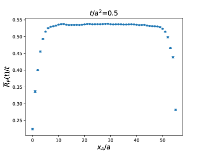
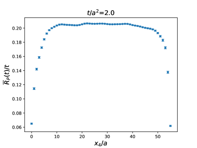
Figure 1: $\overline{R}_{P}(t)/t$ defined in Eq. (17) and determine on the ensemble $A_{3}$ (see Table 1) for values of the flow time $t/a^{2}=0.5,2.0$, corresponding to a flow time radius $r_{f}=\sqrt{8t}=2a,4a$.

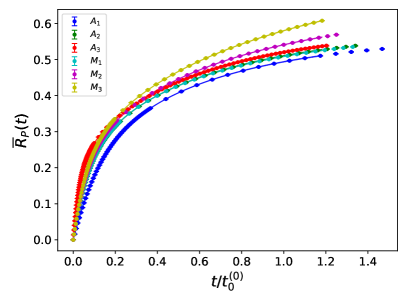
Figure 2: Flow time dependence of the ratio $\overline{R}_{P}$ for all our ensembles. For the x-axis we choose the standard definition of $t_{0}/a^{2}$, i.e. $t_{0}=t_{0}^{(0)}$ (see main text).

In Fig. 2 we show the flow time dependence, in unit of $t/t_{0}$, of $\overline{R}_{P}$ for all our ensembles in Table 1. The data allow a smooth interpolation with a cubic spline and we can perform a robust chiral and continuum limit extrapolation with a global fit at fixed values of the flow time.

To assess the uncertainty due to the continuum limit, we have calculated the values of $t_{0}$ for each ensemble, removing tree-level cutoff effects, at different orders in $a^{2}$ [38].

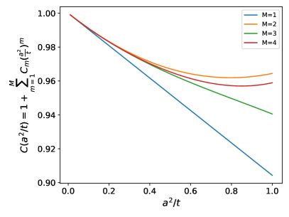
Figure 3: Tree-level lattice artifacts of the energy density defined in Eq. (45) for different orders $(\frac{a^{2}}{t})^{M}$.

Table 2: Here we present the $t_{0}^{(M)}/a^{2}$ values with improvements in Ref. [38], where $M$ is the order of the improvements in $C(a^{2}/t)=1+\sum^{M}_{m=1}C_{m}(\frac{a^{2}}{t})^{m}$.

Designation	$t_{0}^{(0)}/a^{2}$	$t_{0}^{(1)}/a^{2}$	$t_{0}^{(2)}/a^{2}$	$t_{0}^{(3)}/a^{2}$	$t_{0}^{(4)}/a^{2}$
$M_{1}$	2.2586(12)	2.1344(12)	2.1723(12)	2.1655(12)	2.1680(12)
$M_{2}$	2.3993(12)	2.2739(11)	2.3094(11)	2.3033(11)	2.3054(11)
$M_{3}$	2.5371(15)	2.4088(15)	2.4435(15)	2.4379(15)	2.4397(15)
$A_{1}$	1.3627(15)	1.2397(15)	1.3028(14)	1.2849(15)	1.2951(14)
$A_{2}$	2.2378(24)	2.1145(23)	2.1526(23)	2.1457(23)	2.1482(23)
$A_{3}$	4.9879(65)	4.8652(64)	4.8815(64)	4.8802(64)	4.8804(64)

The value of $t_{0}/a^{2}$ determined on a given lattice is usually defined as the value of the flow time satisfying

$$t_{0}^{2}\left\langle E(t_{0})\right\rangle_{\textrm{lat}}=0.3\,,$$ (44)

where $E=\frac{1}{4}G_{\mu\nu}^{a}G_{\mu\nu}^{a}$ and the index “lat” reminds us that the expectation value is evaluated on the lattice. The discretization effects depend on the form of the discretization of $3$ different aspects of the calculation: the lattice action, the lattice GF equation and the lattice definition of the observable which is the energy in this case. By evaluating the energy lattice expectation value at tree-level it is possible to remove tree-level cutoff effects. The tree-level ratio

$$C(t)=\frac{\left\langle E(t)\right\rangle^{(0)}_{\textrm{lat}}}{\left\langle E(t)\right\rangle_{\textrm{c}}^{(0)}}\,,$$ (45)

between the lattice and the continuum expectation values is $1$ in the continuum limit, and dimensionless. At tree-level of perturbation theory, in a pure gauge calculation, the only scale available, beside the lattice spacing $a$, is the flow time $t$, thus $C=C(a^{2}/t)$ and expanding in powers of $a^{2}/t$ one has

$$C(t)=1+\sum_{m=1}^{M}C_{m}\left(\frac{a^{2}}{t}\right)^{m}\,.$$ (46)

The values of the coefficients $C_{m}$, for a wide selection of different lattice actions, GF equations and energy definitions, are given in Ref. [38]. Our choice corresponds to the Iwasaki gauge action, a lattice GF equation using the “plaquette” discretization for the field tensor, and an energy defined using the so called “clover” definition [see Eq. (8)]. We can have different determinations of $t_{0}/a^{2}$

$$\left(t_{0}^{(M)}\right)^{2}\left\langle E(t_{0}^{(M)})\right\rangle_{\textrm{lat}}\times\frac{1}{C(t_{0}^{(M)})}=0.3\,,$$ (47)

depending on the order in $a^{2}/t$ to which we evaluate $C(t)$. In Table 2 we list all the values of $t_{0}/a^{2}$ we have determined for all the ensembles and in Fig. 3 we show the ratio $C(t)$ for given orders $M$ and for our lattice setup. The complete Symanzik analysis of the O($a^{2}$) for flowed gauge observable can be found in Ref. [34].

We can now perform the chiral and continuum extrapolation of the renormalized coupling defined as

$$\overline{g}^{2}=\frac{16\pi^{2}}{3}t^{2}\left\langle E(t)\right\rangle\,,$$ (48)

at fixed values of $t/t_{0}$ and using different definitions of $t_{0}/a^{2}$. We parametrize our data with

$$\left[\overline{g}^{2}\right]_{\textrm{fit}}=A_{g}(t)+B_{g}(t)a^{2}+C_{g}(t)m_{q}+D_{g}(t)m_{q}^{2}\,,$$ (49)

where $X_{g}(t)$, $X=A,B,C,D$, are the fit parameters. We keep the freedom to have both cutoff effects and the quark mass term depending on the flow time, but we do not have sufficient ensembles to be sensitive to mass dependent cutoff effects. The quark mass is determined with the PCAC relation (28).

Figure 4: Simultaneous fit for chiral and continuum extrapolation of renormalized coupling $\overline{g}^{2}$ at $t/t_{0}=0.4$ choosing the standard definition of $t_{0}$ with $M=0$. See main text for more details. The empty point at the coarser lattice spacing is excluded from the continuum and chiral extrapolation.

In Fig. 4 we show the results of our global fits for the coupling $\overline{g}^{2}$ at fixed values of $t/t_{0}=0.4$. In the left plot we show the continuum extrapolation for the standard definition of $t_{0}$, i.e. with $C(t)=1$, while on the right plot we show the chiral extrapolation. The variation of the results obtained for different choices of $t_{0}/a^{2}$ represents our estimate of the systematic uncertainty of the continuum extrapolation. We can now repeat the same analysis for the ratio $\overline{R}_{P}$ of Eq. (17). We parametrize our data with the function

$$\left[\overline{R}_{P}\right]_{\textrm{fit}}=A_{R}(t)+B_{R}(t)a^{2}+C_{R}(t)m_{q}+D_{R}(t)m_{q}^{2}\,,$$ (50)

where $X_{R}(t)$, $X=A,B,C,D$, are the fit parameters. In Fig. 5 we show respectively the continuum limit (left plot) and the chiral extrapolation (right plot) at fixed $t/t_{0}=0.4$ using the standard definition of $t_{0}/a^{2}$ with $C(t)=1$.

Figure 5: Global fit of the ratio $\overline{R}_{P}$ for the definition of $t_{0}$, with $M=0$. See main text for more details. The empty point at the coarser lattice spacing is excluded from the continuum and chiral extrapolation.

Having determined both $\overline{R}_{P}(t)$ and $\overline{g}(t)$ in the continuum limit, we can analyze the dependence of $\Delta(\overline{g}^{2})$ as a function of the renormalized coupling and compare it with perturbation theory. We have calculated using continuum perturbation theory at order O($\overline{g}^{2}$) the same $\Delta(\overline{g}^{2})$. Details of the calculation can be found in Appendix C. The final result at O($\overline{g}^{2}$), consistent with our previous determination [23], is given by

$$\Delta^{(1)}\overline{g}^{2}=\frac{1}{2\pi^{2}}\overline{g}^{2}\,,$$ (51)

and is represented in Fig. 6 by a green straight line. In Fig. 6 we also show our raw data, obtained with the $M=4$ definition of $t_{0}/a^{2}$, and the continuum extrapolation. The raw data show statistical uncertainties in both the y- and x-directions, the latter coming from the uncertainty on the determination of $\overline{g}^{2}$. The blue band represents the statistical and systematic uncertainty in the continuum extrapolation obtained considering the maximal variation of results varying among all the values of $M=0,\ldots,4$. The plot shows the data and our continuum extrapolation for values above the renormalized coupling $\overline{g}^{2}\simeq 9$. The reason for this choice stems from our ability to control the continuum limit, which for smaller values of $\overline{g}^{2}$ become increasingly difficult due to larger cutoff effects.

Figure 6: Blue band corresponds to chiral, continuum limit of data. The error is obtained from the maximum difference between $t_{0}^{(M)}$, $M=0,1,2,3,4$. For plotting $\overline{g}^{2}$ for data points are obtained using $t_{0}^{(4)}$.

Figure 7: Error bands are obtained from the fitting of the chiral, continuum limit data. The error band is obtained from the maximum difference between the fitting results of extrapolated data using different $t_{0}^{(M)}$, $M=0,1,2,3,4$.

Table 3: Results for the polynomial fit $\Delta(\overline{g}^{2})$ as a function of $\overline{g}^{2}$. The perturbative result is given by $\Delta^{(1)}=\frac{1}{2\pi^{2}}=0.05066$.

$\Delta(\overline{g}^{2})=\Delta^{(1)}\overline{g}^{2}+\Delta^{(2)}\overline{g}^{4}+\Delta^{(3)}\overline{g}^{6}+\Delta^{(4)}\overline{g}^{8}$
M	$\Delta^{(1)}$	$\Delta^{(2)}$	$\Delta^{(3)}$	$\Delta^{(4)}$	$\chi^{2}/d.o.f.$	d.o.f.
0	0.07255(71)	-0.00279(17)	0.000027(11)	0.00000059(25)	0.003	785
1	0.08156(55)	-0.00444(13)	0.0001289(85)	-0.00000155(18)	0.0004	815
2	0.0491(10)	0.00191(23)	-0.000286(16)	0.00000749(35)	0.13	874
3	0.07357(66)	-0.00304(16)	0.000046(10)	0.00000012(22)	0.001	833
4	0.0409(11)	0.00376(27)	-0.000420(19)	0.00001063(43)	0.45	888
$\Delta(\overline{g}^{2})=\frac{1}{2\pi^{2}}\overline{g}^{2}+\Delta^{(2)}\overline{g}^{4}+\Delta^{(3)}\overline{g}^{6}+\Delta^{(4)}\overline{g}^{8}$
M	$\Delta^{(2)}$	$\Delta^{(3)}$	$\Delta^{(4)}$	$\chi^{2}/d.o.f.$	d.o.f.
0	0.002321(44)	-0.0003604(46)	0.00001016(14)	0.40	786
1	0.002611(46)	-0.0003923(46)	0.00001097(14)	1.09	816
2	0.001551(38)	-0.0002593(44)	0.00000683(14)	0.13	875
3	0.002210(42)	-0.0003444(43)	0.00000955(13)	0.59	834
4	0.001489(38)	-0.0002493(45)	0.00000647(14)	0.57	889
$\Delta(\overline{g}^{2})=\frac{1}{2\pi^{2}}\overline{g}^{2}+\Delta^{(2)}\overline{g}^{4}+\Delta^{(3)}\overline{g}^{6}+\Delta^{(4)}\overline{g}^{8}+\Delta^{(5)}\overline{g}^{10}$
M	$\Delta^{(2)}$	$\Delta^{(3)}$	$\Delta^{(4)}$	$\Delta^{(5)}$	$\chi^{2}/d.o.f.$	d.o.f.
0	0.004075(68)	-0.000765(14)	0.0000405(10)	-0.000000743(22)	0.005	785
1	0.005016(62)	-0.000934(12)	0.00005056(80)	-0.000000941(18)	0.04	815
2	0.001565(86)	-0.000262(20)	0.0000071(14)	-0.000000005(30)	0.13	874
3	0.004007(63)	-0.000751(13)	0.00003944(88)	-0.000000714(19)	0.01	833
4	0.00095(10)	-0.000126(22)	-0.0000027(16)	0.000000221(36)	0.51	888

This behavior is expected at such short distances, but perhaps surprisingly, as we can see from Fig. 6, we are still able to match the perturbative results even at these relatively large values of the renormalized coupling. We then attempt to parametrize the dependence on the renormalized coupling of $\Delta(\overline{g}^{2})$ over the whole range of renormalized couplings with polynomials of the form

$$\Delta(\overline{g}^{2})=\sum_{i=1}^{N}\Delta^{(i)}\overline{g}^{2i}\,,\qquad N=4,5\,.$$ (52)

In Fig. 7 we show the results of these polynomial fits: for $N=4$ we compare the results leaving the leading O($\overline{g}^{2}$) coefficient as a free fit parameter (left plot), while in the middle plot with constrain it to our perturbative results. From the plots and the fit results in Table 3 we observe that without constraining the fit parameter $\Delta^{(1)}$, we obtain results consistent with one-loop perturbation theory if we consider the uncertainties due to the continuum limit. We also notice that the value for $M=2$ is perfectly consistent with the perturbative result. In the right plot of Fig. 7 we show the same fit up to the order O($\overline{g}^{10}$). The blue bands represent the uncertainty stemming from the uncertainty in the continuum limit. The fit parameters and their uncertainties are given in Table 3. The results indicate a very good description of the numerical data combined with the perturbative results and demonstrate a rather fast convergence of the polynomial. There is still some instabilities in the fit parameters, especially when changing the order of the polynomial (however the $M=2$ case shows very stable results). As our final result we quote the parametrization with $N=4$. This curve is universal and renormalization group invariant. It can be applied to any determination of the expansion coefficient of the pseudoscalar density and to any corresponding hadronic matrix element.

IV.2 Analysis in terms of the bare coupling

A second strategy to study the behavior of the qCEDM at small flow time is to define an effective expansion coefficient $c_{\chi}$ in Eq. (23) and determine its value in terms of the bare coupling. To estimate $c_{\chi}$, as discussed in Sec. II, we want to determine the ratio $R_{P}(t)$ in Eq. (43). The calculation of the correlation functions in (7) and (10) requires the same propagators used in the analysis presented in the previous section. The only difference is that in the denominator of $R_{P}$ we do not flow the quark propagators.

In Fig. 8, we show the source-sink separation, $x_{4}$, dependence of $R_{P}(x_{4};t)/t$ for several values of the flow time $t/a^{2}=0,0.5,2.0$, corresponding to values of the flow time radius $r_{f}=\sqrt{8t}=0,2a,4a$.

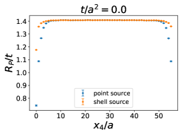
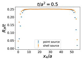
Figure 8: The ratio $R_{P}/t$ defined in Eqs. (11, 43) and determine on the ensemble $A_{3}$ (see Table 1) for several values of the flow time $t/a^{2}=0,0.5,2.0$, corresponding to a flow time radius $r_{f}=\sqrt{8t}=0,2a,4a$. Different colors correspond to different sources.

We observe that the asymptotic plateau value is reached with no particular problem for every value of the flow time we adopt in this work. In Fig. 8 we also show a comparison between a point and a gauge-invariant Gaussian smeared source [39, 40] with $64$ iterations of the smearing algorithm and, using the definition of Ref. [39], a smearing parameter of $\alpha=0.39$. The determination of the plateau is fairly straightforward so we perform a simple constant fit, where the fit range is determined in a standard way minimizing the corresponding $\chi^{2}$.

The result of the fit is the ratio $R_{P}(t)$ of Eq. (43) and it is shown, as a function of $t/t_{0}$, in the left plot of Fig. 9. We determine $t_{0}/a^{2}$ in a standard way [11] and the values for all our ensembles are given in Appendix B in Table 4.

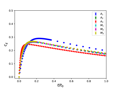
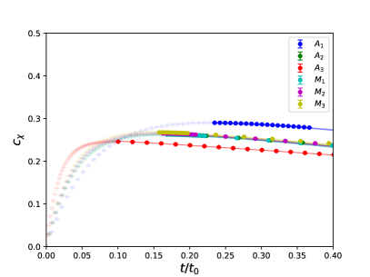
Figure 9: Ratio $R_{P}$ in Eqs. (11, 43) as a function of $t/t_{0}$. In the right plot, error bands are reconstructed based on the final fitting results and solid data points are belonged in the selected fitting ranges in Table 4.

The flow time dependence of $R_{P}(t)$ in Fig. 9 can be explained as follows: at short distances $r_{f}\lesssim 2a$ the ratio $R_{P}$ is dominated by cutoff effects, while at large flow times, aside from the expansion coefficient we want to determine, $R_{P}$ contains contributions from higher dimensional operators linear in $t$. For this reason we decided to perform a simple fit using the fit function

$$R_{\textrm{fit}}(t)=B_{-1}\frac{t_{0}}{t}+B_{0}+B_{1}\frac{t}{t_{0}}\,,$$ (53)

where $B_{-1}$ parametrizes O($a^{2}$/t) effects, while $B_{1}$ parametrizes collectively effects from higher dimensional operators. A similar analysis has been done in Refs. [41, 42, 43] to analyze finite temperature quantities and renormalized 4-fermion operators. The fit coefficient $B_{0}$ provides the value of $c_{\chi}$ in Eq. (23) for each ensemble.

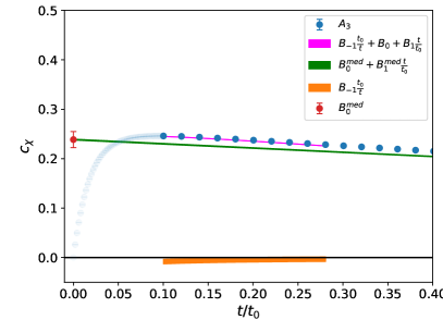
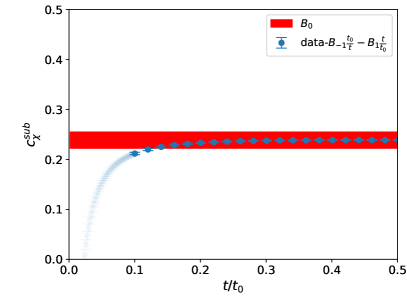
Figure 10: Left plot: flow-time dependence of $c_{\chi}$ for the ensemble $A_{3}$. The different colored lines show the following contributions. Magenta: example of a single fit satisfying the p-value condition. The magenta band represents the statistical uncertainty for the particular fit range chosen. Orange: the contribution of the cutoff effect, parametrized by $B_{-1}$, to the single fit chosen in the plot. The orange band represents the associated statistical and systematic uncertainties stemming from the variation of the fit ranges. Green: the fit result obtained removing cutoff effects. The central value this time represents the median of the distribution obtained varying the fit ranges and satisfying our p-value condition (see Appendix B). The width of the band represents the associated statistical uncertainty. Red data point: the central value is $B_{0}$ obtained as the median of the distribution of values of $B_{0}$ varying the fit ranges and the error represents the sum in quadrature of the statistical and systematic uncertainties on $B_{0}$. Right plot: the blue data points represent the raw data after subtracting the cutoff effects and the higher dimensional operator contributions, linear in $t/t_{0}$, determined from the fit. The red band represents our estimate of $c_{\chi}$ including the statistical and systematic uncertainties added in quadrature.

The efficacy of the method depends on the robustness of the determination of $B_{0}$ with respect to the other contributions. To include all possible systematic effects in the determination of $B_{0}$, we scan many possible fit ranges in $t/t_{0}$ determining both the $\chi^{2}$ and the p-values.

All the details of the analysis are deferred to Appendix B. The value of $B_{0}$, for each ensemble, is determined taking into account the statistical uncertainty and the systematic one stemming from the choice of the fitting range in $t/t_{0}$ (see Appendix B). In the right plot of Fig. 9 we show the effective coefficient $c_{\chi}$ as a function of $t/t_{0}$ for all our ensembles together with the fit functions, where with the thick symbols we show the data included in the fit. We note that the data are described well by the fit function (53). We also note that closer to the continuum limit we are able to describe the data at smaller values of $t/t_{0}$. This is consistent with the expectation that at smaller lattice spacing short distance effects are milder.

In Fig. 10 we show an example of the study of the flow time dependence of $c_{\chi}$. In the left plot with the magenta band we indicate a single fit using Eq. (53) with the associated statistical uncertainty. With the orange band we show only the contribution from the cutoff effects, proportional to $B_{-1}$, this time including the systematic uncertainties stemming from varying the fit ranges. The green line is the fit result obtained removing cutoff effects. The central value this time represents the median of the distribution obtained varying the fit ranges and satisfying our p-value condition (see Appendix B). The width of the band represents the associated statistical uncertainty. The red data point has a central value representing $B_{0}$ obtained as the median of the distribution of values of $B_{0}$ varying the fit ranges and the error represents the sum in quadrature of the statistical and systematic uncertainties. We observe that cutoff effects become important at $t/t_{0}<0.1$ while the fit function describes the data over a large range of flow times, $0.1<t/t_{0}<0.3$. The analysis described in Appendix B also shows that more fit ranges are statistical acceptable and our final error budget include the systematic error induced by varying the fit ranges. A similar behavior is observed for the other ensembles with different fit ranges.

In the right plot of Fig. 10 we show the data for $c_{\chi}$ after subtracting the contributions from cutoff effects and higher dimensional operators

$$c_{\chi}^{\textrm{sub}}(t)=c_{\chi}(t)-B_{-1}\frac{t_{0}}{t}-B_{1}\frac{t}{t_{0}}\,.$$ (54)

The red band now represents our estimate of $c_{\chi}$ including systematic uncertainties and clearly covers any possible ambiguity coming from the choice of the fit range and it coincides with the red point in the left plot. The systematic uncertainties we associate to $B_{0}$ come from the different choices of fit ranges. Again details are given in Appendix B.

Figure 11: Nonperturbative dependence of $c_{\chi}$ as a function of the bare coupling $g_{0}$. The blue band represents the Padé approximant in Eq. (56). The width of the band represents the statistical and systematic uncertainties added in quadrature.

While for the coefficient $B_{0}$ it is not possible to perform the continuum limit because the value of $Z_{\chi}$ is not known, we can nevertheless parametrize the dependence of $c_{\chi}$ on the bare coupling $g_{0}$ with a Padé approximant.

To make sure that the behavior at small coupling is reproduced, we have calculated in perturbation theory the same ratio $R_{P}$ in Eq. (11). The result of the calculation is described in Appendix C. At one loop in perturbation theory there is no contribution to the expansion coefficient $c_{\textrm{CP}}$ coming from the renormalization of the flowed fermion field or the pseudoscalar density. For completeness we quote here the result

$$c_{\chi}=c_{\chi}^{(1)}g^{2}+O(g^{4})\,,\quad c_{\chi}^{(1)}(t)=\frac{1}{2\pi^{2}}\,.$$ (55)

In Fig. 11 the data points represent the nonperturbative determination of $c_{\chi}$ with error bars including statistical and systematic uncertainties. We have parametrized the dependence on the bare coupling of $c_{\chi}$ with a Padé approximant

$$c_{\chi}(g_{0}^{2})=\frac{\frac{1}{2\pi^{2}}g_{0}^{2}+c_{2}g_{0}^{4}}{1+c_{4}g_{0}^{2}}\,,$$ (56)

where we have constrained the leading order in $g_{0}^{2}$ to be consistent with perturbation theory. The green straight line in Fig. 11 represents the perturbative result described in Appendix C, consistent with the result of Ref. [23]. The blue curve represents the Padé approximant obtained from fitting to data we obtained all our ensembles. We note that in some ensembles, for example $M_{3}$, the data became bimodal in distribution and because of this we restricted our fitting to a smaller range in $t/t_{0}$. Otherwise we use the full possible fitting range, when possible, consistent with the p-values chosen. See Appendix B for details. Our final result is summarized by Eq. (56) with the values

$$c_{2}=-0.01115(63)\,,\qquad c_{4}=-0.2690(61)\,.$$ (57)

The parametrization of Eq. (56) with the fit parameters in Eq. (57) provides the coefficient of the power divergence for each value of the bare coupling for the particular choice of the lattice action in this paper. With a different lattice action $c_{\chi}(g_{0}^{2})$ changes, but this paper provides a general method that can be adapted to any lattice action.

V O($a$) improvement at finite flow time

In Sec. III we concluded that to nonperturbatively remove O($a$) cutoff effects in the flowed correlation functions we use, beside improving the action and the local operators, we need to add nonstandard O($a$) terms like $\widetilde{\Gamma}_{PP}(x_{4};t)$ and $\widetilde{\Gamma}_{CP}(x_{4};t)$ defined in Eqs. (40, 37). The numerical determination of these types of correlation functions requires, in addition to the calculation of flowed propagators, the calculation of “kernel” lines, where the Lagrange multipliers $\lambda$ and $\overline{\lambda}$ are contracted with flowed fermion fields. Details on how to determine “kernel” lines are given in Appendix A.

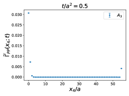
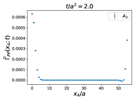
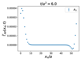
Figure 12: Euclidean time, $x_{4}$, dependence of $\widetilde{\Gamma}_{PP}(x_{4};t)$ for the ensemble $A_{3}$ at $3$ values of the flow time.

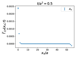
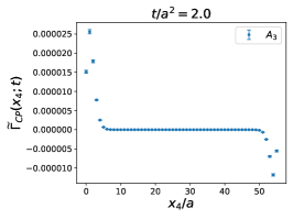
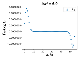
Figure 13: Euclidean time, $x_{4}$, dependence of $\widetilde{\Gamma}_{CP}(x_{4};t)$ for the ensemble $A_{3}$ at $3$ values of the flow time.

In Figs. (12, 13) we show the Euclidean time dependence, $x_{4}$, respectively of $\widetilde{\Gamma}_{PP}(x_{4};t)$ and $\widetilde{\Gamma}_{CP}(x_{4};t)$ for the ensemble $A_{3}$ and $3$ values of the flow time $t/a^{2}=0.5,2.0,6.0$. It is clear that any nonzero contribution is localized in the region $x_{4}\lesssim\sqrt{8t}$ while for $x_{4}\gg\sqrt{8t}$ the correlation functions vanish. We conclude that as far as $x_{4}\gg\sqrt{8t}$ our determination is nonperturbatively O($a$) improved up to small O($amg^{2}$) terms. This result, obtained with minimal numerical effort, is one of the great advantages of using the gradient flow to renormalize higher dimensional operators.

VI Summary and Outlook

When a $CP$-violating signal is measured in electric dipole moment experiments in the future, it will be imperative that theory provides guidance on the origins of this measured violation. As the sources themselves can come from various BSM scenarios, it is important to understand the systematics of each source and its ensuing impact on observables.

To that end we have analyzed the quark chromo-EDM operator, for the first time using the gradient flow method to provide control on the power divergences that occur due to mixing during renormalization when using a discrete spacetime regulator. In essence, our gradient flow analysis trades induced power divergences with cutoff dependencies, the latter being much more amenable to a continuum limit extrapolation.

Our most important result is shown in Fig. 7 and the corresponding description in Eqs. (52). In the plots we show the nonperturbative determination of the finite renormalization connecting, for a wide range of renormalized coupling values, the qCEDM operator with the pseudoscalar density at finite flow time. The calculation of this finite renormalization reduces the power divergence problem to the determination of the nonperturbative evolution of the pseudoscalar density at finite flow time. Once a nonperturbative determination of the expansion coefficient of the pseudoscalar density is available, it is possible to determine, nonperturbatively and in the continuum, not only of the leading power divergences but also the subleading logarithmic corrections to the power divergences. In view of the increased precision of lattice data it becomes critical to control also this subleading corrections and work in this direction is in progress.

The scheme defined in this work, even if technically difficult, can also be used in perturbation theory allowing a matching at high-energy and in Appendix C we show the detail of the calculation. For completeness we also perform an analysis in terms of the bare coupling, where the dependence of the power divergence coefficient is reconstructed using a Padé approximant. We emphasize that the analysis in terms of the bare coupling, and the corresponding Padé approximant, depends on the lattice action used.

We have also discussed the O($a$) improvement of the qCEDM and the appropriate modifications at finite flow time. We conclude that the improvement is greatly simplified using the gradient flow definition of the qCEDM.

We consider this work as a first nonperturbative solution of the problem of the power divergences for the qCEDM. The method we develop in this paper can be adopted for any local operator mixing with lower dimensional operators and with any lattice action.

Appendix A FLOWING FERMION FIELDS

Here we elaborate on the fermion and Lagrange multiplier fields we use in our work. The standard lattice QCD quark propagator

$$\left[\psi(x)\overline{\psi}(y)\right]_{F}=S(x,y)\,,$$ (58)

where $\left[\cdot\right]_{F}$ denotes a fermionic field contractions, represents the usual inverse of the lattice QCD action with a given source $\eta(x)$. The propagators are flowed as described, for example, in [11]:

$$\left[\chi(x;t)\overline{\psi}(y)\right]_{F}=a^{4}\sum_{v}K(x,t;v,0)S(v,y)\,,$$ (59)

$$\left[\psi(x)\overline{\chi}(y;s)\right]_{F}=a^{4}\sum_{v}S(x,v)K(y,s;v,0)^{\dagger}\,,$$ (60)

where the kernel $K$ is the solution of the equation

$$\left(\partial_{t}-D^{x}_{\mu}D^{x}_{\mu}\right)K(x,t;y,s)=0\,,$$

$$K(x,y;t,t)=\frac{1}{a^{4}}\delta_{xy}\,.$$ (61)

The flowed propagators are used to determine the correlators in Eqs. (7, 18).

In order to compute the correlation functions in Eqs. (37, 40), parametrizing specific O($a$) terms for flowed correlation functions, we need to flow the Lagrange fields $\lambda(x;t)$ in the following manner,

$$\left[\chi(x;t)\overline{\lambda}(y;0)\right]_{F}=a^{4}\sum_{v}\delta_{xv}K(v,t;y,\epsilon)\,,$$ (62)

$$\left[\lambda(x;0)\overline{\chi}(y;s)\right]_{F}=a^{4}\sum_{v}K(v,s;x,\epsilon)^{\dagger}\delta_{vy}\,,$$ (63)

where $\delta_{xy}$ is a Kronecker delta in spacetime, color, and spin indices. The numerical calculation proceeds similarly as in the case of flowed propagators, with a point source as initial condition of the flow equation.

As an example we show explicitly the contractions for the correlation function in Eq. (37)

$$\widetilde{\Gamma}_{CP}(x_{4};t) = a^{3}\sum_{{\bf x}}\left\langle O_{\textrm{C}}^{ij}(x_{4},{\bf x};t)\widetilde{P}^{ji}(0,{\bf 0};0)\right\rangle=$$ (64)

$$= a^{3}\sum_{{\bf x}}\left\langle\bigg{[}\overline{\chi}(x_{4},{\bf x};t)\gamma_{5}\sigma_{\mu\nu}G_{\mu\nu}(x_{4},{\bf x};t)\chi(x_{0},{\bf x};t)\right.$$

$$\times \left.\big{(}\overline{\lambda}(0,{\bf 0};0)\gamma_{5}\psi(0,{\bf 0};0)+\overline{\psi}(0,{\bf 0};0)\gamma_{5}\lambda(0,{\bf 0};0)\big{)}\bigg{]}\right\rangle$$

$$= -a^{3}\sum_{{\bf x}}{\rm{Tr}}\bigg{[}[\psi(0,{\bf 0};0)\overline{\chi}(x_{4},{\bf x};t)]_{F}\gamma_{5}\sigma_{\mu\nu}G_{\mu\nu}(x_{4},{\bf x};t)[\chi(x_{4},{\bf x};t)\overline{\lambda}(0,{\bf 0};0)]_{F}\gamma_{5}\bigg{]}$$

$$- {\rm{Tr}}\bigg{[}[\lambda(0,{\bf 0};0)\overline{\chi}(x_{4},{\bf x};t)]_{F}\gamma_{5}\sigma_{\mu\nu}G_{\mu\nu}(x_{4},{\bf x};t)[\chi(x_{4},{\bf x};t)\overline{\psi}(0,{\bf 0};0)]_{F}\gamma_{5}\bigg{]}\,,$$

where with $[\cdot]_{F}$ we denote a fermionic contraction.

Appendix B DETAILS ON DATA ANALYSIS

In this Appendix we discuss in more details the analysis presented in Sec. IV.2. The data in Fig. 9 and the fit functional form in Eq. (53) suggest to restrict the fit ranges using $t/t_{0}$ larger than the value corresponding to the maximum value of $R_{P}/t$. We then fit in all ranges between $(t/t_{0})_{\textrm{min}}$ and $(t/t_{0})_{\textrm{max}}$ given in Table 4, keeping always a minimum number of $5$ data points.

Table 4: $t_{0}/a^{2}$ and fit ranges for each ensemble. In the 3rd and 4th column we show the complete fit ranges, $(t/t_{0})_{\text{min/max}}$, while in the 5th and 6th we show the fit ranges after analyzing the p-values of the fits (see main text in this Appendix).

Designation	$t_{0}/a^{2}$	range of $(t/t_{0})_{\text{min}}$	range of $(t/t_{0})_{\text{max}}$	range of $(t/t_{0})^{\text{sel}}_{\text{min}}$	range of $(t/t_{0})^{\text{sel}}_{\text{max}}$
$M_{1}$	2.2586(12)	(0.1682, 0.7525)	(0.1903, 0.9738)	(0.1682, 0.2656)	(0.1903, 0.4869)
$M_{2}$	2.3993(12)	(0.1624, 0.7500)	(0.1833, 0.9583)	(0.1624, 0.2500)	(0.1833, 0.4167)
$M_{3}$	2.5371(15)	(0.1576, 0.7881)	(0.1773, 0.9851)	(0.1576, 0.2758)	(0.1773, 0.5123)
$A_{1}$	1.3627(15)	(0.2348, 0.5870)	(0.2715, 0.9539)	(0.2348, 0.5870)	(0.2715, 0.9539)
$A_{2}$	2.2378(24)	(0.1697, 0.7594)	(0.1921, 0.9827)	(0.1697, 0.2680)	(0.1921, 0.4914)
$A_{3}$	4.9879(65)	(0.1002, 0.8820)	(0.2005, 0.9822)	(0.1002, 0.8820)	(0.2005, 0.9822)

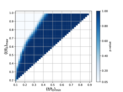
(a) $A_{3}$ ensemble

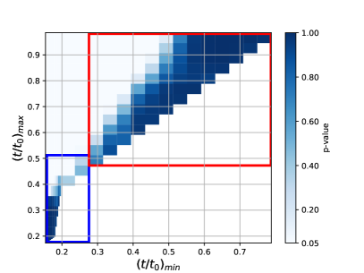
(b) $M_{3}$ ensemble

Figure 14: p-values obtained from the $\chi^{2}/\text{d.o.f}$. The darker regions correspond to the acceptable fit ranges. In the right plot, the blue and red rectangles correspond to blue and red peak in Fig. 15. See main text in this Appendix.

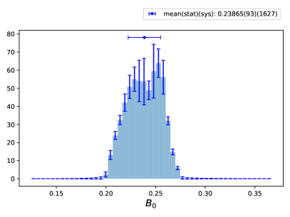
(a) $A_{3}$ ensemble

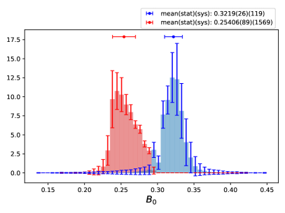
(b) $M_{3}$ ensemble

Figure 15: Distribution of the fit parameter $B_{0}$ for all the fit ranges satisfying $p>0.05$.

To select the acceptable fit ranges and the corresponding values of the fit parameters we scan the $\chi^{2}$ and the p-values for each fit, using central values and statistical errors obtained by a standard bootstrap analysis of the raw data. The analysis shows $2$ typical behaviors for the fit parameters, that can be exemplified plotting a heat map of the p-values for different fit ranges in the $2$ representative ensembles $A_{3}$ and $M_{3}$ (see Fig. 14). While for $A_{3}$, the lattice spacing closer to the continuum limit, we observe a stable values for the fit parameters for a wide choice of fit ranges, for the ensemble $M_{3}$ we observe $2$ well separated regions where the null hypothesis is not rejected: a fit range region at small flow time (blue box) and one at larger flow time (red box).

To analyze the distributions of the fit parameters obtained, we first generate $N_{B}=1000$ bootstrap samples of the raw data and perform $N_{B}$ fits for each fit range selected by the p-value condition. In this way we have the values of $B_{0,-1,1}$ with the corresponding bootstrap uncertainties for each fit range. We then take each value of the fit parameters and plot a histogram with the distribution obtained changing the fit ranges. This is equivalent to generating $N_{B}=1000$ slightly different histograms, showing the distribution of the fit parameters with varying fit ranges. We then take each bin of each histogram and perform a standard bootstrap analysis obtaining for each bin a central value with a statistical fluctuation. These histograms are shown in Figs. 15 for the ensembles $A_{3}$ (left plot) and $M_{3}$ (right plot). They are a summary of the statistical and systematic uncertainties giving a visual representation of the systematic uncertainty stemming from the choice of the fit ranges, and for each bin the statistical uncertainty.

We then proceed to determine the median of each histogram obtained for each bootstrap sample. This gives us $N_{B}$ bootstrap values for the median: a standard statistical analysis gives us the central value and the associate statistical error. To determine the systematic uncertainty we take the median of the summary histograms, like the ones in Figs. 15, and determine symmetrically around the median the region with $68\%$ of the area of the normalized distribution. The statistical and systematic errors are then summed in quadrature and are shown on top of the histograms in Fig. 15.

We notice that in the right plot of Fig. 15 we have clearly a two-peak structure. A deeper investigation of the origin of the $2$ peaks is revealed when we separate $2$ very distinct regions in the flow time dependence of $c_{\chi}$. This is transparent when we analyze the heat map in the right plot of Fig. 14. We clearly notice that the p-value prefers $2$ very distinct regions in the fit ranges. It turns out that the $2$ distinct regions clearly correspond to the $2$ peaks in the right plot of Fig. 15. For the ensemble $M_{3}$, right plots, we draw in blue and red the values of the $B_{0}$ obtained in the region isolated with the heat maps, i.e. red for fit ranges at “large” values of $t/t_{0}$ and blue for fit ranges at “small” values of $t/t_{0}$. Instead for the ensemble $A_{3}$ we observe that all fit ranges, satisfying the p-value condition, give values of $B_{0}$ all within a seemingly well defined distribution (see left plot of Fig. 15).

The values of $c_{\chi}$ we plot in Fig. 11 correspond to the fit ranges selected by the p-values condition, and the selection of small flow time fit ranges explained above. For the ensembles $A_{1}$ and $A_{3}$ we take every fit range selected by the p-value condition. While choosing the same fit ranges for all the ensembles will give us a smaller total uncertainties in the fit parameters, we consider for the ensemble $A_{1}$ and $A_{3}$, that do not show a double peak structure, the larger range of fit intervals providing us with a more conservative estimate of the total uncertainty.

The results for $B_{0}$ are used to estimate $c_{\chi}$ of Fig. 11. For the other $2$ fit parameters in Fig. 16, we plot the lattice spacing dependence of the fit parameter $B_{-1}$ and $B_{1}$. It is reassuring to notice that $B_{-1}$ practically vanishes at a lattice spacing of $a\simeq 0.65$ fm, indicating small discretization errors. We also find that the contributions of the higher dimensional operators, proportional to $B_{1}$, are not negligible, and will be the focus of forthcoming publications.

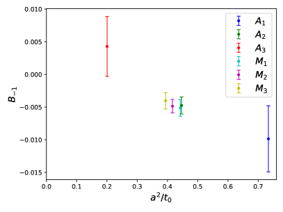
(a) Fit parameter $B_{-1}$

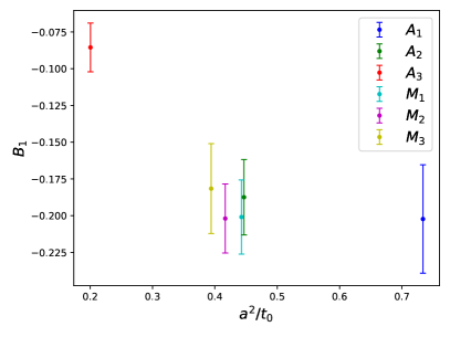
(b) Fit parameter $B_{1}$

Figure 16: These results are $t_{0}/a^{2}$ dependence of each fitting parameters $B_{-1}$, $B_{1}$. With the exception of the $A_{1}$ and $A_{3}$ ensembles, the data points for each ensemble were computed from the fitting ranges from peak and splitting positions given in Table 4.

Appendix C PERTURBATIVE CALCULATION OF $c_{\textrm{CP}}$

In this Appendix we detail the perturbative calculation of the power divergent coefficient in perturbation theory. We refer to [23] for the details of the short flow time expansion (SFTE) of the qCEDM with $2$ external quarks. For now, we simply summarize the relevant results. Near the $t=0$ boundary, we may reconstruct the flowed qCEDM in a basis $\mathcal{A}$ of gauge-invariant, $CP$-violating local operators with a modified operator-product expansion:

$$O^{R}_{C}(x;t)\stackrel{{\scriptstyle t\rightarrow 0}}{{\sim}}\sum_{\mathcal{A}}c_{Ci}(t)O^{R}_{i}(x;0),$$ (65)

where all of the flow time dependence of the expanded operator is encoded strictly by the Wilson coefficients $c_{Ci}$. For the qCEDM, for which $[O_{C}]=d+1$, the leading order contribution comes from the pseudoscalar density,

$$O_{P}(x;t)=P(x;t)=\overline{\chi}(x;t)\gamma_{5}\chi(x;t),$$ (66)

which has canonical dimension $[O_{P}]=d-1$. s (In what follows, note that with respect to [23] we have fixed the normalization of the pseudoscalar density and qCEDM operators such that $k_{P}=1$ and $k_{C}=-i$.) Consequently, we expect a linear divergence in the flow time. We may then write

$$O^{R}_{C}(x;t)=c_{CP}(t)P^{R}(x;0)+\cdots,$$ (67)

where the ellipsis signifies contributions from higher-dimensional operators. The leading contribution to the mixing coefficient appears at one-loop order and is easily extracted by studying the correlation function $G_{C}(x,y;t)=\int_{z\in\mathbb{R}^{d}}\langle\overline{\psi}(x)O_{C}(z;t)\psi(y)\rangle$ at ${\mathcal{O}}(g^{2})$. We quote our previous result [23]:

$$c^{(1)}_{CP}(t)=6\frac{C_{2}(F)}{(4\pi)^{2}}\frac{1}{t}.$$ (68)

We may, however, extract the same coefficient by studying Eq. (11) in perturbation theory, where the nature of the SFTE demands that the coupling be arbitrarily small:

$$c_{CP}(t)=\frac{1}{t}\lim_{x_{4}\rightarrow\infty}[R_{P}(x_{4};t)]_{R},$$ (69)

where

$$\left[R_{P}(x_{4};t)\right]_{R}=t\frac{\left[\Gamma_{CP}(x_{4};t)\right]_{R}}{\left[\Gamma_{PP}(x_{4})\right]_{R}}\,,$$ (70)

where we adopt for continuum correlation functions the same notation as for the lattice ones (cf. Eqs. (7, 10)).

This is a manifestly gauge-invariant scheme, and the separation of the two operators in Euclidean time ensures that the correlation function is ground-state dominated. Thus it is naturally more amenable to a lattice implementation.

Figure 17: The only contribution to $\Gamma_{PP}(x_{4};t)$ at tree level.

We work in dimensionally regularized Euclidean space at leading order. The denominator of Eq. (70) generates a single one-loop diagram (Fig. 17), which is easily evaluated directly

$$\Gamma_{PP}^{(0)}(x_{4};0)=-4\frac{\dim(F)}{(4\pi)^{2}}\frac{1}{x_{4}^{3}}.$$ (71)

The spacing $x_{d}$ provides an ultraviolet cutoff, so that the above correlator converges as $d\rightarrow 4^{\pm}$ (hence $x_{d}\rightarrow x_{4}$).

Turning our attention to the numerator, we study $\int_{\textbf{x}\in\mathbb{R}^{d-1}}\langle O_{C}(\textbf{x},x_{d};t)P(0;0)\rangle$, where the pseudoscalar density is fixed at the origin as allowed by translational symmetry. The leading contributions in this case are three two-loop “vacuum bubbles,” pictured in Fig. 18.

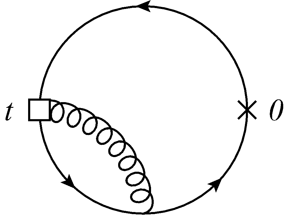
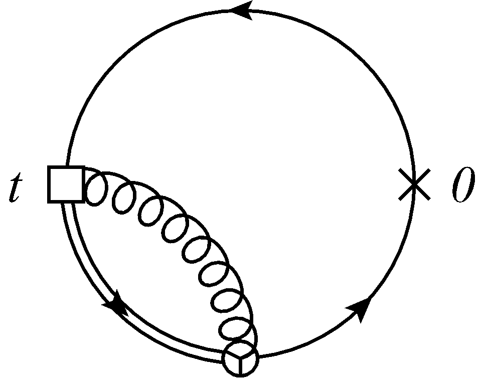
Figure 18: Leading-order contributions to $\Gamma_{CP}(x_{4};t)$.

Since the Euclidean time coordinate is not integrated, it is tempting to proceed directly in position space for that component, transforming only the spatial coordinates to momentum space. Instead, we have found that the simplest method is to inject some momentum $q$ into both operators, proceed as usual in momentum space, and pass back to real space only at the end, projecting the spatial momentum q to zero. Summarily:

$$\Gamma_{CP}^{(1)}(x_{d};t)=\lim_{p\rightarrow 0}\int_{\mathbb{R}^{d-1}}d^{d-1}x\ e^{-ipx}\int_{q}e^{iqx}\tilde{\Gamma}_{CP}^{(1)}(q;t),$$ (72)

where $\tilde{\Gamma}_{CP}(q;t)$ is the Fourier transform of $\Gamma_{CP}(x;t)$. As it turns out, the relevant integrals in this case all converge in four dimensions, so we implicitly take the $d\rightarrow 4$ limit in what follows. The middle and right diagrams in Fig. 18 trivially and identically vanish. For the left diagram in Fig. 18, we insert the one-loop result of the analogous calculation with two external quarks (Eq. (34a) from [23]), which we denote here with $\widetilde{G}_{C}^{(1)}(p;t)$. Without expanding in $t$ we obtain

$$\widetilde{G}_{C}^{(1)}(p;t)=3\frac{C_{2}(F)}{(4\pi)^{2}}\frac{1}{t}\cdot\tilde{f}(p^{2}t)\gamma_{5},$$ (73)

where

$$\tilde{f}(z)=2\left\{\frac{z}{2}\text{E}_{1}\left(\frac{z}{2}\right)-z\text{E}_{1}\left(z\right)+\frac{1-z}{z}\left(e^{-z/2}-e^{-z}\right)\right\}$$ (74)

is a common function in flowed perturbation theory, and $E_{n}(z)$ is the generalized exponential integral. Then, closing the gauge-invariant vacuum diagram around a pseudoscalar density operator at the origin, we have

$$\tilde{\Gamma}_{CP}^{(1)}(q;t)=2\cdot{\rm{Tr}}\int_{p}\frac{\not{p}}{p^{2}}\tilde{G}_{C}^{(1)}(p;t)\frac{\not{p}-\not{q}}{(p-q)^{2}}e^{-(p-q)^{2}t}+{\mathcal{O}}(g^{4}).$$ (75)

Using standard techniques, we arrive at

$$\tilde{\Gamma}_{CP}^{(1)}(q;t)=-12\frac{C_{2}(F)\dim(F)}{(4\pi)^{4}t^{2}}\tilde{g}(q^{2}t),$$ (76)

where

$$\tilde{g}(z)=\begin{aligned} \frac{1}{3z}\Bigg{\{}&(3z^{2}+12z-3)e^{-z}-(6z^{2}+30z-12)e^{-\frac{z}{2}}+(3z^{2}+18z-9)e^{-\frac{z}{3}}\\ &-(3z^{3}+15z^{2}+16z)E_{1}(z)+(3z^{3}+21z^{2}+12z)E_{1}\left(\frac{z}{2}\right)\\ &-(z^{3}+9z^{2}+6z)E_{1}\left(\frac{z}{3}\right)\Bigg{\}}.\end{aligned}$$ (77)

Finally, we Fourier transform this result to find

$$\Gamma_{CP}^{(1)}(x_{4};t)=-12\frac{C_{2}(F)\dim(F)}{(4\pi)^{4}t^{2}}\cdot t^{-1/2}g(t^{-1/2}x_{4}),$$ (78)

where

$$g(\epsilon)=\frac{1}{2\epsilon^{5}}\begin{aligned} \Bigg{\{}&(\epsilon^{6}-4\epsilon^{4}+20\epsilon^{2}-48)\text{erf}\left(\frac{1}{2}\epsilon\right)-(4\epsilon^{6}-8\epsilon^{4}+28\epsilon^{2}-48)\text{erf}\left(\frac{\sqrt{2}}{2}\epsilon\right)\\ &+(3\epsilon^{6}-4\epsilon^{4}+12\epsilon^{2}-16)\text{erf}\left(\frac{\sqrt{3}}{2}\epsilon\right)+\frac{2}{\sqrt{\pi}}\Big{[}e^{-\frac{1}{4}\epsilon^{2}}(\epsilon^{5}-6\epsilon^{3}+24\epsilon)\\ &-\sqrt{2}e^{-\frac{1}{4}(\sqrt{2}\epsilon)^{2}}(2\epsilon^{5}-6\epsilon^{3}+24\epsilon)+\sqrt{3}e^{-\frac{1}{4}(\sqrt{3}\epsilon)^{2}}(\epsilon^{5}-2\epsilon^{3}+8\epsilon)\Big{]}\Bigg{\}}.\end{aligned}$$ (79)

For large argument, the function $g$ goes as

$$g(\epsilon)\stackrel{{\scriptstyle\epsilon\gg 0}}{{\sim}}\frac{2}{\epsilon^{3}}.$$ (80)

and we find that

$$c_{CP}^{(1)}(t)=\lim_{x_{4}\rightarrow\infty}\frac{\Gamma^{(1)}_{CP}(x_{4};t)}{\Gamma^{(0)}_{PP}(x_{4})}=6\frac{C_{2}(F)}{(4\pi)^{2}}\frac{1}{t},$$ (81)

as desired. Indeed, for $N_{c}=3$, we have

$$c_{CP}^{(1)}(t)=\frac{1}{2\pi^{2}t}$$ (82)

as in Eq. (6). For completeness, we remark that the same leading-order result may be obtained with the ratio

$$\Delta(\bar{g}^{2})=\lim_{x_{4}\rightarrow\infty}t\ \frac{\Gamma_{CP}(x_{4};t)}{\Gamma_{PP}(x_{4};t)}\Big{|}_{t=\textrm{constant}}\,,$$ (83)

in which now one of the pseudoscalar density operators in the denominator is fixed at $t$, and the renormalized coupling $\bar{g}$ is taken to be an implicit function of $t$. Since the self-mixing of the flowed pseudoscalar density is unity at leading order, we may for now safely ignore the $\textrm{log}\ t$ corrections, which are suppressed by the coupling. We find that

$$\Gamma_{PP}^{(0)}(x_{4};t)=-2\frac{\dim(F)}{(4\pi)^{2}t}\cdot t^{-1/2}f(t^{-1/2}x_{4}),$$ (84)

where

$$t^{-1/2}f(\epsilon)=\begin{aligned} t^{-1/2}\cdot\frac{1}{\epsilon^{3}}\bigg{\{}&\left(\epsilon^{4}+4\right)\text{erf}\left(\frac{\epsilon}{2}\right)-\left(\epsilon^{4}+2\right)\text{erf}\left(\frac{\epsilon}{\sqrt{2}}\right)\\ &-\frac{1}{\sqrt{\pi}}\left[\left(\epsilon^{3}-2\epsilon\right)\left(\sqrt{2}e^{-\frac{1}{4}(\sqrt{2}\epsilon)^{2}}-2e^{-\frac{1}{4}(\epsilon)^{2}}\right)\right]\bigg{\}}\end{aligned}$$ (85)

is the inverse Fourier transform of Eq. (74). Again, we have

$$f(\epsilon)\stackrel{{\scriptstyle\epsilon\gg 0}}{{\sim}}\frac{2}{\epsilon^{3}},$$ (86)

so that

$$\Delta^{(1)}=\lim_{x_{4}\rightarrow\infty}t\ \frac{\Gamma_{CP}^{(1)}(x_{4};t)}{\Gamma_{PP}^{(0)}(x_{4};t)}\Big{|}_{t=\textrm{constant}}=6\frac{C_{2}(F)}{(4\pi)^{2}}\cdot\lim_{\epsilon\rightarrow\infty}\frac{g(\epsilon)}{f(\epsilon)}=6\frac{C_{2}(F)}{(4\pi)^{2}}\xrightarrow{N_{c}\rightarrow 3}\frac{1}{2\pi^{2}}$$ (87)

as in Eq. (51).

It is clear from the calculation described above that the leading-order contribution to the power divergence is universal whether we probe the local operator with external quarks (cf. Eq. (6) and Ref. [23]) or with a pseudoscalar density. This should be expected, since the SFTE is an operator-level relation, and fluctuations are neglected at leading order. Moreover, this confirms $c_{P}^{(0)}(t)=1+{\mathcal{O}}(t)$, which follows trivially from the perturbative solution to the fermionic flow equations. The universality property, however, strongly depends on the condition that $x_{4}$ is much larger than $\sqrt{8t}$. This is somehow expected as well, because no additional contact terms are present when both $t\rightarrow 0$ and $x_{4}\rightarrow 0$ with this kinematical choice; viz, the qCEDM and the pseudoscalar density do not form a local operator product so long as the physical separation is well larger than the smearing radius. We have indeed repeated the calculation presented in this appendix integrating Eq. (72) over the whole spacetime volume, thus including also the region at $x_{4}\sim 0$, obtaining a different result.

References

- Fields et al. [2020] B. D. Fields, K. A. Olive, T.-H. Yeh, and C. Young, Big-Bang Nucleosynthesis after Planck, J. Cosmol. Astropart. Phys. 03, 010, [Erratum: J. Cosmol. Astropart. Phys. 11, E02 (2020)], arXiv:1912.01132 [astro-ph.CO] .
- Tanabashi et al. [2018] M. Tanabashi et al. (Particle Data Group), Review of Particle Physics, Phys. Rev. D 98, 030001 (2018).
- Jungman et al. [1996] G. Jungman, M. Kamionkowski, A. Kosowsky, and D. N. Spergel, Cosmological parameter determination with microwave background maps, Phys. Rev. D 54, 1332 (1996), arXiv:astro-ph/9512139 .
- Aghanim et al. [2020] N. Aghanim et al. (Planck Collaboration), Planck 2018 results. VI. Cosmological parameters, Astron. Astrophys. 641, A6 (2020), [Erratum: Astron.Astrophys. 652, C4 (2021)], arXiv:1807.06209 [astro-ph.CO] .
- Zyla et al. [2020] P. Zyla et al. (Particle Data Group), Review of Particle Physics, PTEP 2020, 083C01 (2020).
- Shaposhnikov [1987] M. Shaposhnikov, Baryon Asymmetry of the Universe in Standard Electroweak Theory, Nucl. Phys. B 287, 757 (1987).
- Gavela et al. [1994] M. Gavela, P. Hernandez, J. Orloff, and O. Pene, Standard model CP violation and baryon asymmetry, Mod. Phys. Lett. A 9, 795 (1994), arXiv:hep-ph/9312215 .
- Huet and Sather [1995] P. Huet and E. Sather, Electroweak baryogenesis and standard model CP violation, Phys. Rev. D 51, 379 (1995), arXiv:hep-ph/9404302 .
- Abel et al. [2020] C. Abel et al. (nEDM Collaboration), Measurement of the permanent electric dipole moment of the neutron, Phys. Rev. Lett. 124, 081803 (2020), arXiv:2001.11966 [hep-ex] .
- Seng [2015] C.-Y. Seng, Reexamination of The Standard Model Nucleon Electric Dipole Moment, Phys. Rev. C91, 025502 (2015), arXiv:1411.1476 [hep-ph] .
- Lüscher [2010] M. Lüscher, Properties and uses of the Wilson flow in lattice QCD, JHEP 1008, 071, arXiv:1006.4518 [hep-lat] .
- Lüscher and Weisz [2011] M. Lüscher and P. Weisz, Perturbative analysis of the gradient flow in non-abelian gauge theories, JHEP 1102, 051, arXiv:1101.0963 [hep-th] .
- Lüscher [2013] M. Lüscher, Chiral symmetry and the Yang–Mills gradient flow, JHEP 1304, 123, arXiv:1302.5246 [hep-lat] .
- Lüscher [2014] M. Lüscher, Future applications of the Yang-Mills gradient flow in lattice QCD, PoS LATTICE2013, 016 (2014), arXiv:1308.5598 [hep-lat] .
- Constantinou et al. [2015] M. Constantinou, M. Costa, R. Frezzotti, V. Lubicz, G. Martinelli, D. Meloni, H. Panagopoulos, and S. Simula, Renormalization of the chromomagnetic operator on the lattice, Phys. Rev. D 92, 034505 (2015), arXiv:1506.00361 [hep-lat] .
- Shindler [2014] A. Shindler, Chiral Ward identities, automatic O(a) improvement and the gradient flow, Nucl.Phys. B881, 71 (2014), arXiv:1312.4908 [hep-lat] .
- Iwasaki [1985] Y. Iwasaki, Renormalization Group Analysis of Lattice Theories and Improved Lattice Action: Two-Dimensional Nonlinear O(N) Sigma Model, Nucl. Phys. B 258, 141 (1985).
- Sheikholeslami and Wohlert [1985] B. Sheikholeslami and R. Wohlert, Improved Continuum Limit Lattice Action for QCD with Wilson Fermions, Nucl. Phys. B 259, 572 (1985).
- Lüscher et al. [1996] M. Lüscher, S. Sint, R. Sommer, and P. Weisz, Chiral symmetry and O(a) improvement in lattice QCD, Nucl. Phys. B 478, 365 (1996), arXiv:hep-lat/9605038 .
- Lüscher et al. [1997] M. Lüscher, S. Sint, R. Sommer, P. Weisz, and U. Wolff, Nonperturbative O(a) improvement of lattice QCD, Nucl. Phys. B 491, 323 (1997), arXiv:hep-lat/9609035 .
- Shindler et al. [2015] A. Shindler, T. Luu, and J. de Vries, Nucleon electric dipole moment with the gradient flow: The -term contribution, Phys. Rev. D92, 094518 (2015), arXiv:1507.02343 [hep-lat] .
- Dragos et al. [2021] J. Dragos, T. Luu, A. Shindler, J. de Vries, and A. Yousif, Confirming the Existence of the strong CP Problem in Lattice QCD with the Gradient Flow, Phys. Rev. C 103, 015202 (2021), arXiv:1902.03254 [hep-lat] .
- Rizik et al. [2020] M. D. Rizik, C. J. Monahan, and A. Shindler, Short flow-time coefficients of CP-violating operators, Phys. Rev. D 102, 034509 (2020), arXiv:2005.04199 [hep-lat] .
- Suzuki [2013] H. Suzuki, Energy–momentum tensor from the Yang–Mills gradient flow, PTEP 2013, 083B03 (2013), arXiv:1304.0533 [hep-lat] .
- Makino and Suzuki [2014] H. Makino and H. Suzuki, Lattice energy–momentum tensor from the Yang–Mills gradient flow—inclusion of fermion fields, PTEP 2014, 063B02 (2014), [Erratum: PTEP 2015, 079202 (2015)], arXiv:1403.4772 [hep-lat] .
- Endo et al. [2015] T. Endo, K. Hieda, D. Miura, and H. Suzuki, Universal formula for the flavor non-singlet axial-vector current from the gradient flow, PTEP 2015, 053B03 (2015), arXiv:1502.01809 [hep-lat] .
- Hieda and Suzuki [2016] K. Hieda and H. Suzuki, Small flow-time representation of fermion bilinear operators, Mod. Phys. Lett. A31, 1650214 (2016), arXiv:1606.04193 [hep-lat] .
- Shindler [2021] A. Shindler, Flavor-diagonal CP violation: the electric dipole moment, Eur. Phys. J. A 57, 128 (2021).
- Bhattacharya et al. [2015] T. Bhattacharya, V. Cirigliano, R. Gupta, E. Mereghetti, and B. Yoon, Dimension-5 CP-odd operators: QCD mixing and renormalization, Phys. Rev. D92, 114026 (2015), arXiv:1502.07325 [hep-ph] .
- Jenkins et al. [2018] E. E. Jenkins, A. V. Manohar, and P. Stoffer, Low-Energy Effective Field Theory below the Electroweak Scale: Anomalous Dimensions, JHEP 01, 084, arXiv:1711.05270 [hep-ph] .
- Aoki et al. [2010] S. Aoki et al. (PACS-CS Collaboration), Non-perturbative renormalization of quark mass in QCD with the Schroedinger functional scheme, JHEP 08, 101, arXiv:1006.1164 [hep-lat] .
- Symanzik [1983a] K. Symanzik, Continuum Limit and Improved Action in Lattice Theories. 1. Principles and Theory, Nucl. Phys. B 226, 187 (1983a).
- Symanzik [1983b] K. Symanzik, Continuum Limit and Improved Action in Lattice Theories. 2. O(N) Nonlinear Sigma Model in Perturbation Theory, Nucl. Phys. B 226, 205 (1983b).
- Ramos and Sint [2016] A. Ramos and S. Sint, Symanzik improvement of the gradient flow in lattice gauge theories, Eur. Phys. J. C76, 15 (2016), arXiv:1508.05552 [hep-lat] .
- Beckett et al. [2011] M. G. Beckett, P. Coddington, B. Joó, C. M. Maynard, D. Pleiter, O. Tatebe, and T. Yoshie, Building the international lattice data grid, Computer Physics Communications 182, 1208 (2011).
- Aoki et al. [2009] S. Aoki et al. (PACS-CS Collaboration), 2+1 Flavor Lattice QCD toward the Physical Point, Phys. Rev. D79, 034503 (2009), arXiv:0807.1661 [hep-lat] .
- Aoki et al. [2006] S. Aoki, M. Fukugita, S. Hashimoto, K.-I. Ishikawa, Y. Iwasaki, K. Kanaya, et al. (CP-PACS, JLQCD Collaboration), Nonperturbative O(a) improvement of the Wilson quark action with the RG-improved gauge action using the Schrodinger functional method, Phys. Rev. D 73, 034501 (2006), arXiv:hep-lat/0508031 .
- Fodor et al. [2014] Z. Fodor, K. Holland, J. Kuti, S. Mondal, D. Nogradi, and C. H. Wong, The lattice gradient flow at tree-level and its improvement, JHEP 09, 018, arXiv:1406.0827 [hep-lat] .
- Gusken [1990] S. Gusken, A Study of smearing techniques for hadron correlation functions, Lattice 89. Proceedings, Symposium on Lattice Field Theory, Capri, Italy, Sep 18-21, 1989, Nucl. Phys. Proc. Suppl. 17, 361 (1990).
- Alexandrou et al. [1991] C. Alexandrou, F. Jegerlehner, S. Gusken, K. Schilling, and R. Sommer, B meson properties from lattice QCD, Phys. Lett. B256, 60 (1991).
- Kitazawa et al. [2016] M. Kitazawa, T. Iritani, M. Asakawa, T. Hatsuda, and H. Suzuki, Equation of State for SU(3) Gauge Theory via the Energy-Momentum Tensor under Gradient Flow, Phys. Rev. D94, 114512 (2016), arXiv:1610.07810 [hep-lat] .
- Iritani et al. [2019] T. Iritani, M. Kitazawa, H. Suzuki, and H. Takaura, Thermodynamics in quenched QCD: energy–momentum tensor with two-loop order coefficients in the gradient-flow formalism, PTEP 2019, 023B02 (2019), arXiv:1812.06444 [hep-lat] .
- Suzuki et al. [2020] A. Suzuki, Y. Taniguchi, H. Suzuki, and K. Kanaya, Four quark operators for kaon bag parameter with gradient flow, Phys. Rev. D 102, 034508 (2020), arXiv:2006.06999 [hep-lat] .
- Jülich Supercomputing Centre [2018] Jülich Supercomputing Centre, JURECA: Modular supercomputer at Jülich Supercomputing Centre, Journal of large-scale research facilities 4, A132 (2018).
- Towns et al. [2014] J. Towns et al., XSEDE: Accelerating Scientific Discovery, Comput. Sci. Eng. 16, 62 (2014).