Non Gaussian Denoising Diffusion Models

Abstract

Generative diffusion processes are an emerging and effective tool for image and speech generation. In the existing methods, the underline noise distribution of the diffusion process is Gaussian noise. However, fitting distributions with more degrees of freedom, could help the performance of such generative models. In this work, we investigate other types of noise distribution for the diffusion process. Specifically, we show that noise from Gamma distribution provides improved results for image and speech generation. Moreover, we show that using a mixture of Gaussian noise variables in the diffusion process improves the performance over a diffusion process that is based on a single distribution. Our approach preserves the ability to efficiently sample state in the training diffusion process while using Gamma noise and a mixture of noise.

1 Introduction

Deep generative neural networks has shown significant progress over the last years. The main architectures for generation are: (i) VAE kingma2013auto based, for example, NVAE vahdat2020nvae and VQ-VAE razavi2019generating , (ii) GAN goodfellow2014generative based, for example, StyleGAN karras2020analyzing for vision application and WaveGAN donahue2018adversarial for speech (iii) Flow-based, for example Glow kingma2018glow (iv) Autoregessive, for example, Wavenet for speech oord2016wavenet and (v) Diffusion Probabilistic Models sohl2015deep , for example, Denoising Diffusion Probabilistic Models (DDPM) ho2020denoising and its implicit version DDIM song_denoising_2020 .

Models from this last family have shown significant progress in generation capabilities during the last years, e.g., sohl2015deep ; ho2020denoising ; chen_wavegrad_2020 ; kong_diffwave_2020 , and have achieved comparable results to the state of the art generation architecture in both images and speech.

A DDPM is a Markov chain of latent variables. Two processes are modeled: (i) a diffusion process and (ii) a denoising process. During training, the diffusion process learns to transform data samples into Gaussian noise. The denoising is the reverse process and it is used during inference to generate data samples, stating from Gaussian noise. The second process can be condition on attributes to control the generation sample. In order to get high quality synthesis, a large number of denoising steps is used (i.e. $1000$ steps). A notable property of the diffusion process is a closed form formulation of the noise that arises from accumulating diffusion stems. This allows to sampling arbitrary states in the Markov chain of the diffusion process without calculating the previous steps.

In the Gaussian case, this property stems from the fact that adding Gaussian distributions leads to another Gaussian distribution. Other distributions have similar properties. For example, for the Gamma distribution, the sum of two distributions that share the scale parameter is a Gamma distribution of the same scale. The Poisson distribution has a similar property. However, its discrete nature makes it less suitable for DDPM.

In DDPM, the mean of the distribution is set at zero. The Gamma distribution, with its two parameters (shape and scale), is better suited to fit the data than a Gaussian distribution with one degree of freedom (scale). Furthermore, the Gamma distribution generalizes other distributions, and many other distributions can be derived from it leemis2008univariate .

The added modeling capacity of the Gamma distribution can help speed up the convergence of the DDPM model. Consider, for example, conventional DDPM model that were trained with Gaussian noise on the CelebA dataset liu2015faceattributes . After $t$ steps, one can compute the histogram of the differences between the obtained image $x_{t}$ and the original noise image $x_{0}$. Both a Gaussian distribution, Gamma distribution, and a mixture of Gaussian can then be fitted to this histogram, as shown in Fig. 1(a,b,c). Unsurprisingly, for a single step, both the Gaussian distribution and the Gamma distribution can be fitted with the same error, see Fig. 1(d). However, when trying to fit for more than a single step, the Gamma distribution and the mixture of Gaussian becomes a much better fit.

In this paper, we investigate two types of non-Gaussian noise distribution: (i) Mixture of Gaussian, and (ii) Gamma. The two proposed models maintain the property of the diffusion process to sample arbitrary states without calculating the previous steps. Our results are demonstrated in two major domains: vision and audio. In the first domain, the proposed method is shown to provide a better FID score for generated images. For speech data, we show that the proposed method improves various measures, such as Perceptual Evaluation of Speech Quality (PESQ), short-time objective intelligibility (STOI) and Mel-Cepstral Distortion (MCD).

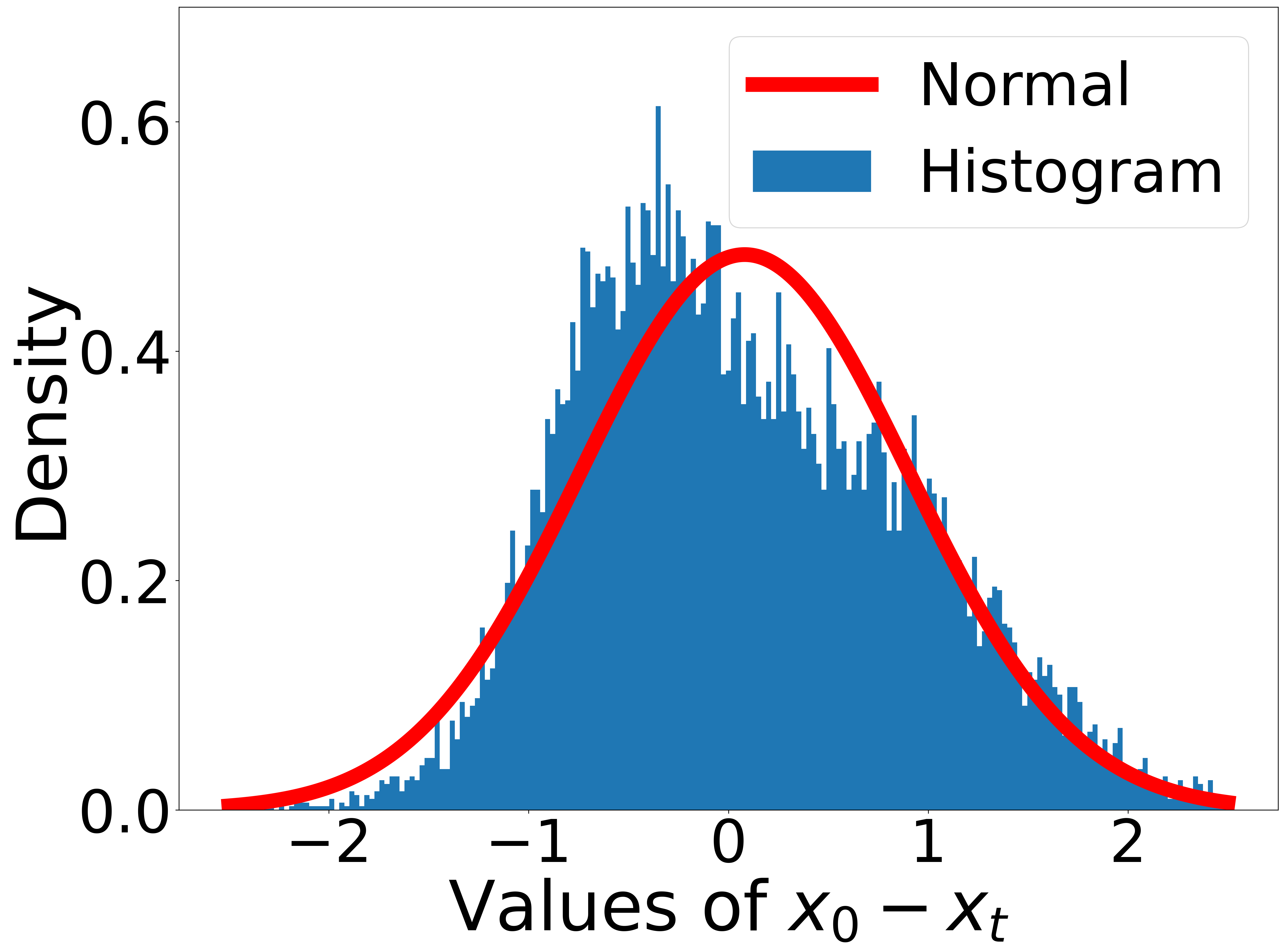
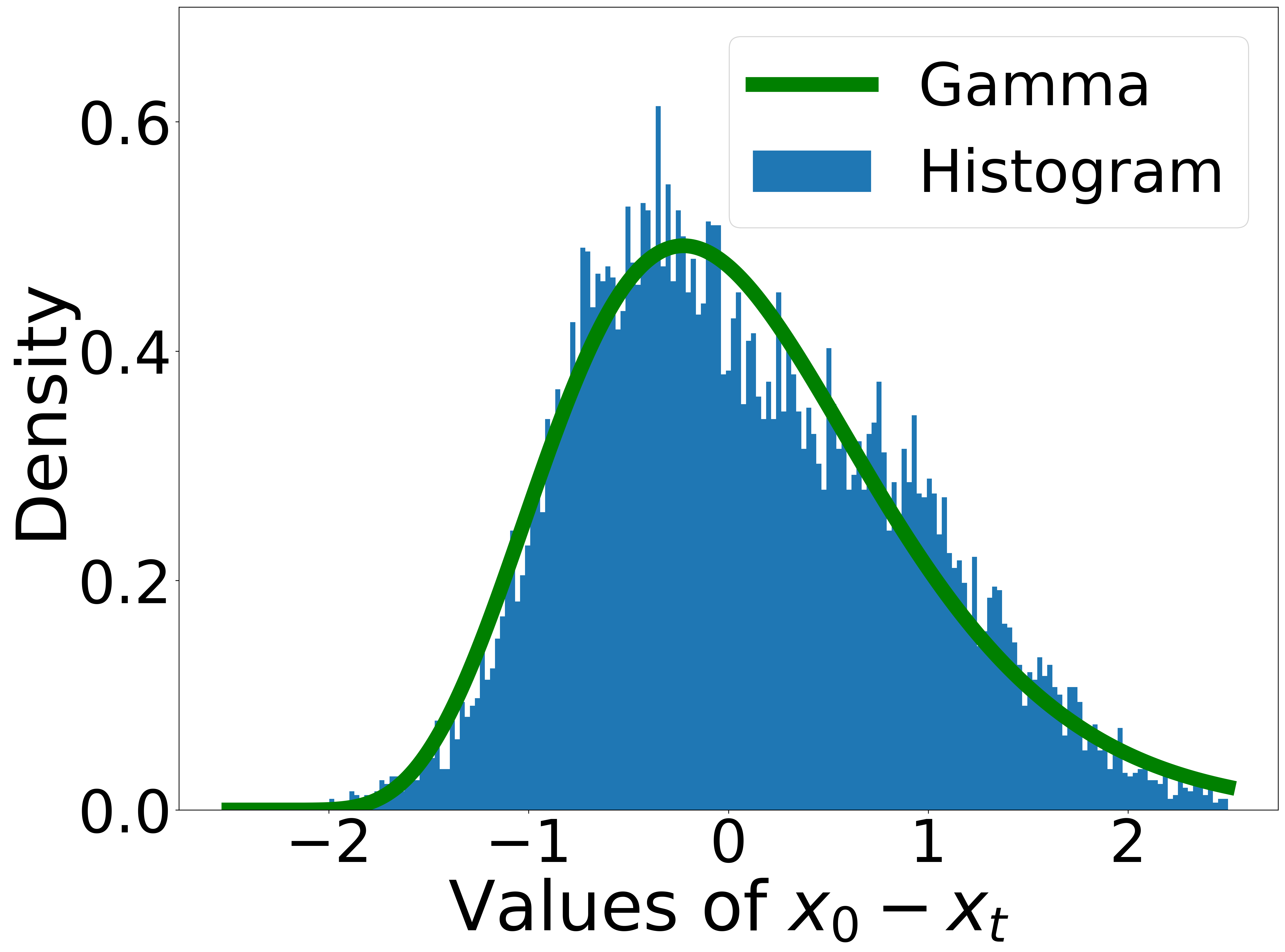
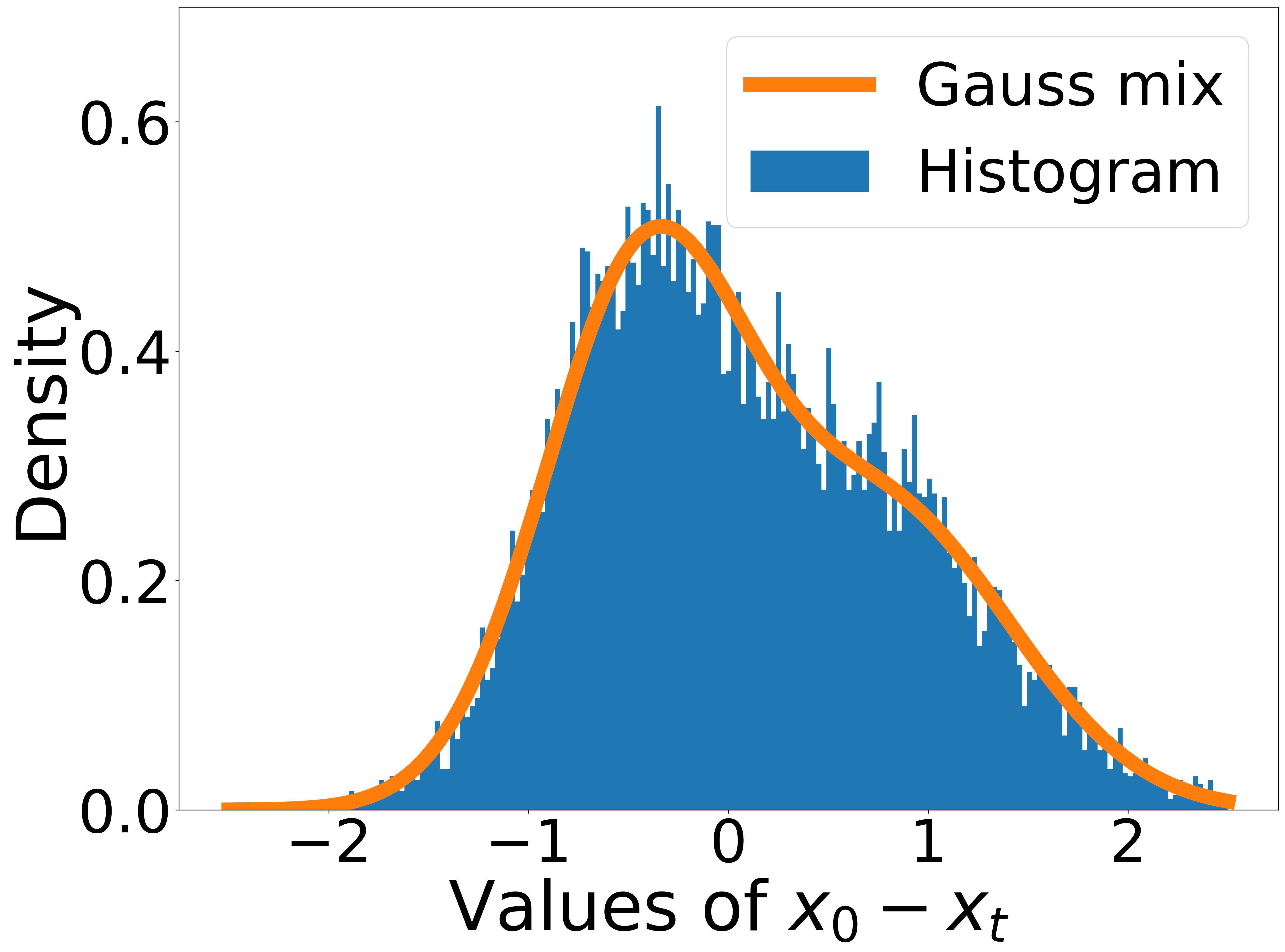
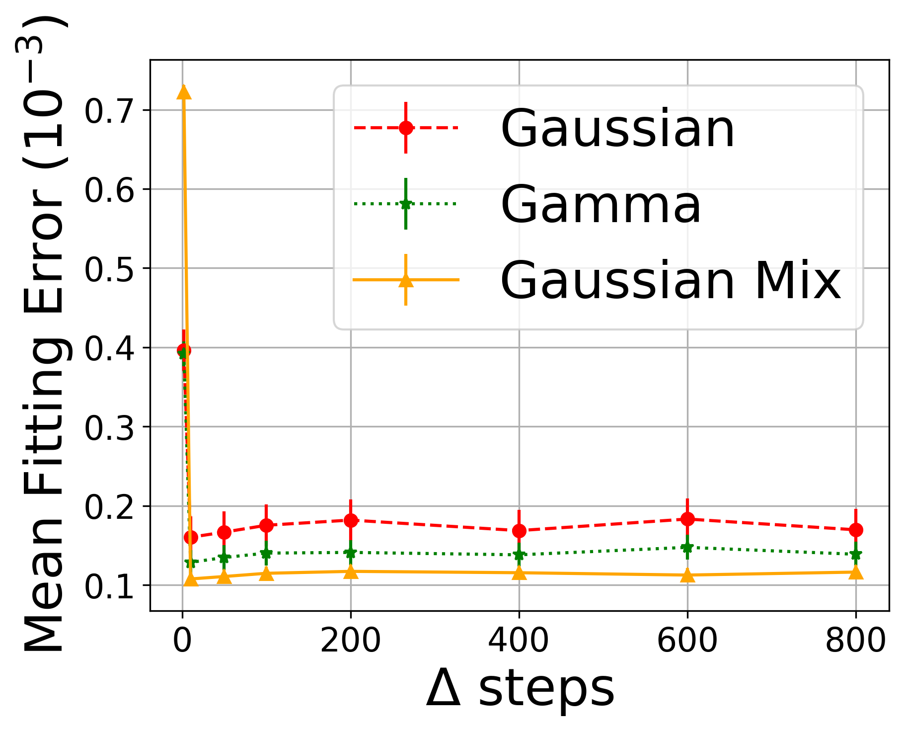
(a)	(b)	(c)	(d)

Figure 1: Fitting a distribution to the histogram of the difference between $x_{0}$ and the image $x_{t}$ after $t$ DDPM steps, using a pretrained (Gaussian) celebA (64x64) model. (a) The fitting of a Gaussian to the histogram of a typical image after $t-50$ steps. (b) Fitting a mixture of Gaussian distribution. (c) Fitting a Gamma distribution. (d) The fitting error to Gaussian and Gamma distribution, measured as the MSE between the histogram and the fitted probability distribution function. Each point is the average value for the generation of $100$ images. The vertical errorbars denote the standard deviation.

2 Related Work

In their seminal work, Sohl-Dickstein et al. introduce the Diffusion Probabilistic Model sohl2015deep . The model is applied to various domains, such as time series and images. The main drawback in the proposed model is the fact that it needs up to thousands of iterative steps in order to generate valid data sample. Song et al. song2019generative proposed a diffusion generative model based on Langevin dynamics and the score matching method hyvarinen2005estimation . The model estimate the Stein score function liu2016kernelized which is the logarithm of the data density. Given the Stein score function, the model can generate data points.

Denoising Diffusion Probabilistic Models (DDPM) ho2020denoising combine generative models based on score matching and neural Diffusion Probabilistic Models into a single model. Similarly, in chen_wavegrad_2020 ; kong2020diffwave a generative neural diffusion process based on score matching was applied to speech generation. These models achieve state of the art results for speech generation, and show superior results over well-established methods, such as Wavernn kalchbrenner2018efficient , Wavenet oord2016wavenet , and GAN-TTS binkowski2019high .

Diffusion Implicit Models (DDIM) is a method to accelerate the denoising process song_denoising_2020 . The model employs a non-Markovian diffusion process to generate higher quality sample. The model helps to reduce the number of diffusion steps, e.g., from a thousand steps to a few hundred.

Song et al. show that score based generative models can be considered as a solution to a stochastic differential equation song2020score . Gao et al. provide an alternative approach to train an energy-based generative model using a diffusion process gao2020learning .

Another line of work in audio is that of neural vocoders that are based on a denoising diffusion process. WaveGrad chen_wavegrad_2020 and DiffWave kong2020diffwave are conditioned on the mel-spectrogram and produce high fidelity audio samples using as few as six step of the diffusion process. These models outperform adversarial non-autoregressive baselines.

Algorithm 1 DDPM training procedure.

1:  Input: dataset $d$, diffusion process length $T$, noise schedule $\beta_{1},...,\beta_{T}$

2:  repeat

3:     $x_{0}\sim d(x_{0})$

4:     $t\sim\mathcal{U}(\{1,...,T\})$

5:     $\varepsilon\sim\mathcal{N}(0,I)$

6:     $x_{t}=\sqrt{\bar{\alpha}_{t}}x_{0}+\sqrt{1-|\bar{\alpha}_{t}|}\varepsilon$

7:     Take gradient descent step on:
$\|\varepsilon-\varepsilon_{\theta}(x_{t},t)\|_{1}$

8:  until converged

Algorithm 2 DDPM sampling algorithm

1:  $x_{T}\sim\mathcal{N}(0,I)$

2:  for t= T, …, 1 do

3:     $z\sim\mathcal{N}(0,I)$

4:     $\hat{\varepsilon}=\varepsilon_{\theta}(x_{t},t)$

5:     $x_{t-1}=\frac{x_{t}-\frac{1-\alpha_{t}}{\sqrt{1-\bar{\alpha}_{t}}}\hat{\varepsilon}}{\sqrt{\alpha_{t}}}$

6:     if $t\neq 1$ then

7:        $x_{t-1}=x_{t-1}+\sigma_{t}z$

8:     end if

9:  end for

10:  return $x_{0}$

3 Diffusion models for Various Distributions

We start by recapitulating the Gaussian case, after which we derive diffusion models for mixtures of Gaussians and for the Gamma distribution.

3.1 Background - Gaussian DDPM

Diffusion network learn the gradients of the data log density

$$s(y)=\nabla_{y}\log p(y)$$ (1)

By using Langevin Dynamics and the gradients of the data log density $\nabla_{y}\log p(y)$, a sample procedure from the probability can be done by:

$$\tilde{y}_{i+1}=\tilde{y}_{i}+\frac{\eta}{2}s(\tilde{y}_{i})+\sqrt{\eta}z_{i}$$ (2)

where $z_{i}\sim\mathcal{N}(0,I)$ and $\eta>0$ is the step size. The diffusion process in DDPM ho2020denoising is defined by a Markov chain that gradually adds Gaussian noise to the data according to a noise schedule. The diffusion process is defined by:

$$q(x_{1:T}|x_{0})=\prod_{t=1}^{T}q(x_{t}|x_{t-1})\,,$$ (3)

where T is the length of the diffusion process, and $x_{T},...,x_{t},x_{t-1},...,x_{0}$ is a sequence of latent variables with the same size as the clean sample $x_{0}$. The Diffusion process is parameterized with a set of parameters called noise schedule ($\beta_{1},\dots\beta_{T}$) that defines the variance of the noise added at each step:

$$q(x_{t}|x_{t-1}):=\mathcal{N}(x_{t};\sqrt{1-\beta_{t}}x_{t-1},\beta_{t}\mathbf{I})\,,$$ (4)

Since we are using Gaussian noise random variable at each step The diffusion process can be simulated for any number of steps with the closed formula:

$$x_{t}=\sqrt{\bar{\alpha}_{t}}x_{0}+\sqrt{1-\bar{\alpha}_{t}}\varepsilon\,,$$ (5)

where $\alpha_{i}=1-\beta_{i}$, $\bar{\alpha}_{t}=\prod_{i=1}^{t}\alpha_{i}$ and $\varepsilon=\mathcal{N}(0,\mathbf{I})$. The complete training procedure is defined in Alg.1. Given the input dataset $d$, the algorithm samples $\epsilon$, $x_{0}$ and $t$. The noisy latent state $x_{t}$ is calculated and fed to the DDPM neural network $\varepsilon_{\theta}$. A gradient descent step is taken in order to estimate the $\varepsilon$ noise with the DDPM network $\varepsilon_{\theta}$.

The inference procedure uses the trained model $\varepsilon_{\theta}$ and a variation of the Langevin dynamics. The following update from song_denoising_2020 is used to reverse a step of the diffusion process:

$$x_{t-1}=\dfrac{x_{t}-\frac{1-\alpha_{t}}{\sqrt{1-\bar{\alpha}_{t}}}\varepsilon_{\theta}(x_{t},t)}{\sqrt{\bar{\alpha}_{t}}}+\sigma_{t}\varepsilon\,,$$ (6)

where $\varepsilon$ is white noise and $\sigma_{t}$ is the standard deviation of added noise. In song_denoising_2020 the authors use ${\sigma_{t}}^{2}=\beta_{t}$. The complete inference algorithm present at Alg. 2. Starting from a Gaussian noise and then step-by-step reversing the diffusion process, by iteratively employing the update rule of Eq. 6.

3.2 Mixture of Gaussian Noise

Eq. 4 can be written as:

$$x_{t}=\sqrt{1-\beta_{t}}x_{t-1}+\sqrt{\beta_{t}}\epsilon_{t}$$ (7)

where $\epsilon_{t}$ is the Gaussian noise of step $t$. This can be generalized by adding a mixture of Gaussians at each step, i.e.,

$$x_{t}=\sqrt{1-\beta_{t}}x_{t-1}+\sqrt{\beta_{t}}(\sum_{i=0}^{C}{z_{i}\epsilon^{i}_{t}})$$ (8)

where $z_{i}$ are boolean random variables and $C$ is the number of Gaussian variables. We denote by $p_{i}$ the probability that $z_{i}=1$ for the $i$ Gaussian variable ($\sum_{i=0}^{C}p_{i}=1$).

For simplicity, we focus on $C=2$, mixtures with an expectation of zero, and two Gaussian distributions with the same variance $\phi_{t}^{2}$ and the same weight ($p=0.5$):

$$x_{t}=\sqrt{1-\beta_{t}}x_{t-1}+\sqrt{\beta_{t}}(b\epsilon^{1}_{t}+(1-b)\epsilon^{2}_{t})\,,$$ (9)

where $\epsilon^{1}_{t}\sim N(m^{1}_{t},{\phi_{t}}^{2})$, $\epsilon^{1}_{t}\sim N(m^{2}_{t},{\phi_{t}}^{2})$ and $b\sim\mathcal{B}ernoulli(p)$. In addition to the zero mean property that we assume, we scale the variables such that the variance of $b\epsilon^{1}_{t}+(1-b)\epsilon^{2}_{t}$ is one.

We reparametrize the added noise at each step as $\sqrt{\beta_{t}}X_{t}$, i.e.

$$X_{t}=b\epsilon^{1}_{t}+(1-b)\epsilon^{2}_{t}\,.$$ (10)

Since $X_{t}$ is zero mean and has a variance of one ($E(X_{t})=0$ and $V(X_{t})=1$), the added value at each step $\sqrt{\beta_{t}}X_{t}$ will have zero mean and a $\beta_{t}$ variance. The following Lemma captures the relation between the two means in this case.

Lemma 1.

Assuming that $\epsilon_{t}^{1}\sim\mathcal{N}(m_{t}^{1},{\phi_{t}}^{2})$, $\epsilon_{t}^{2}\sim\mathcal{N}(m_{t}^{2},{\phi_{t}}^{2})$, $b\sim Bernouilli(p)$, $E(X_{t})=0$ and $V(X_{t})=1$. Then the following equation hold:

$$m_{t}^{1}=\sqrt{\frac{1-{\phi_{t}}^{2}}{p(1-p)+\frac{p^{3}}{1-p}+2p^{2}}}$$ (11)

$$m_{t}^{2}=-\frac{p}{1-p}m_{t}^{1}$$ (12)

Proof.

The mean value of $X_{t}$ can be calculate as:

$$E(X_{t}) =E(b\epsilon^{1}_{t})+E((1-b)\epsilon^{2}_{t})=E(b)E(\epsilon^{1}_{t})+E(1-b)E(\epsilon^{2}_{t})$$

$$=E(b)E(\epsilon^{1}_{t})+E(1-b)E(\epsilon^{2}_{t})=pm_{t}^{1}+(1-p)m_{t}^{2}$$

since $b,\epsilon^{1}_{t},\epsilon^{2}_{t}$ are independent and due to the linearity of the expectation. Since we assume that $E(X_{t})=0$, we have:

$$m_{t}^{2}=-\frac{p}{1-p}m_{t}^{1}$$ (13)

Denote $X^{1}_{t}=b\epsilon^{1}_{t}$ and $X^{2}_{t}=(1-b)\epsilon^{2}_{t}$. The variance of $X_{t}$ is given as:

$$V(X_{t})=V(X^{1}_{t})+V(X^{2}_{t})+2cov(X^{1}_{t},X^{2}_{t})$$ (14)

where $cov(X^{1}_{t},X^{2}_{t})=-E(X^{1}_{t})E(X^{2}_{t})$ since $X^{1}_{t}X^{2}_{t}=0$. Therefore, Eq.14 becomes:

$$V(X_{t})=V(X^{1}_{t})+V(X^{2}_{t})-2E(X^{1}_{t})E(X^{2}_{t})$$ (15)

$V(X^{1}_{t})$ can be calculate as:

$$V(X^{1}_{t}) =V(b\epsilon^{1}_{t})=V(\epsilon^{1}_{t})E(b^{2})+V(b)E(\epsilon^{1}_{t})^{2}={\phi_{t}}^{2}E(b)+p(1-p)({m_{t}^{1}})^{2}$$

$$={\phi_{t}}^{2}p+p(1-p)({m_{t}^{1}})^{2}$$

since $b^{2}=b$. Similarly, we can show that $V(X^{2}_{t})={\phi_{t}}^{2}(1-p)+p(1-p)({m_{t}^{2}})^{2}$. Therefore, we have:

$$V(X_{t}) ={\phi_{t}}^{2}p+p(1-p)({m_{t}^{1}})^{2}+{\phi_{t}}^{2}(1-p)+p(1-p)({m_{t}^{2}})^{2}-2E(X^{1}_{t})E(X^{2}_{t})$$

$$={\phi_{t}}^{2}p+p(1-p)({m_{t}^{1}})^{2}+{\phi_{t}}^{2}(1-p)+p(1-p)({m_{t}^{2}})^{2}-2pm_{t}^{1}(1-p)m_{t}^{2}$$ (16)

Substitute Eq.13 into Eq.16 we have: $V(X_{t})=({m_{t}^{1}})^{2}\left(p(1-p)+\frac{p^{3}}{1-p}+2p^{2}\right)+p{\phi_{t}}^{2}+(1-p){\phi_{t}}^{2}$. Since $V(X_{t})=1$ we have:

$$m_{t}^{1}=\sqrt{\frac{1-{\phi_{t}}^{2}}{p(1-p)+\frac{p^{3}}{1-p}+2p^{2}}}$$ (17)

∎

Denote $\mathcal{M}({\phi_{t}}^{2})$ ($\phi_{t}\in[0,1]$) as the mixture model with two equally weighed Gaussian components, each with a variance of $\phi_{t}^{2}$ and means stated above. The closed form for sampling $x_{t}$ from $x_{0}$ is given by:

$$x_{t}=\sqrt{\bar{\alpha}_{t}}x_{0}+\sqrt{1-\bar{\alpha}_{t}}N_{t}$$ (18)

Where $N_{t}\sim\mathcal{M}({\phi_{t}}^{2})$ and $\phi_{t}$ is a free hyperparameter. Similarly to Eq.6, the inference is given by:

$$x_{t-1}=\dfrac{x_{t}-\frac{1-\alpha_{t}}{\sqrt{1-\bar{\alpha}_{t}}}\varepsilon_{\theta}(x_{t},t)}{\sqrt{\bar{\alpha}_{t}}}+\sigma_{t}N_{t}$$ (19)

The complete training procedure is given in Alg. 3. The input is the standard deviation for each step ($\phi_{t})_{t\in\{1...T\}}$, the dataset $d$, the total number of steps in the diffusion process $T$ and the noise schedule $\beta_{1},...,\beta_{T}$. For each batch, the training algorithm samples an example $x_{0}$, a number of steps $t$ and the noise itself $\varepsilon$. Then it calculates $x_{t}$ from $x_{0}$ by using Eq.18. The neural network $\varepsilon_{\theta}$ has an input $x_{t}$ and is condition on the number of step $t$. A gradient descend step is used to approximate $N_{t}$ with the neural network $\varepsilon_{\theta}$. The main differences from the single Gaussian case (Alg. 1) are the following: (i) calculating the mixture of Gaussian parameters (ii) and sampling $N_{t}$.

The inference procedure is given in Alg. 4. The algorithm starts from a noise $x_{T}$ sampled from $\mathcal{M}({\phi_{T}}^{2})$. Then for $T$ steps the algorithm estimates $x_{t-1}$ from $x_{t}$ by using Eq.19. Note that as in song_denoising_2020 $\sigma_{t}=\beta_{t}$. The main differences from the single Gaussian case (Alg. 2) is the following: (i) the start sampling point $x_{T}$, (ii) and the sampling noise $z$.

Algorithm 3 Mixture of Gaussian Training Algorithm

1:  Input: The standard deviations ($\phi_{t})_{t\in\{1...T\}}$, dataset $d$, diffusion process length $T$, noise schedule $\beta_{1},...,\beta_{T}$

2:  repeat

3:     $x_{0}\sim d(x_{0})$

4:     $t\sim\mathcal{U}(\{1,...,T\})$

5:     $N_{t}\sim\mathcal{M}({\phi_{t}}^{2})$

6:     $x_{t}=\sqrt{\bar{\alpha}_{t}}x_{0}+\sqrt{1-|\bar{\alpha}_{t}|}N_{t}$

7:     Take gradient descent step on:
$\|N_{t}-\varepsilon_{\theta}(x_{t},t)\|_{1}$

8:  until converged

Algorithm 4 Mixture of Gaussian Inference Algorithm

1:  $x_{T}\sim\mathcal{M}({\phi_{T}}^{2})$

2:  for t= T, …, 1 do

3:     $z\sim\mathcal{M}({\phi_{t-1}}^{2})$

4:     $\hat{\varepsilon}=\varepsilon_{\theta}(x_{t},t)$

5:     $x_{t-1}=\frac{x_{t}-\frac{1-\alpha_{t}}{\sqrt{1-\bar{\alpha}_{t}}}\hat{\varepsilon}}{\sqrt{\alpha_{t}}}$

6:     if $t\neq 1$ then

7:        $x_{t-1}=x_{t-1}+\sigma_{t}z$

8:     end if

9:  end for

10:  return $x_{0}$

3.3 Using the Gamma distribution for noise

Denote $\Gamma(k,\theta)$ as the Gamma distribution, where $k$ and $\theta$ are the shape and the scale respectively. We modify Eq. 7 by adding, during the diffusion process, noise that follows a Gamma distribution:

$$x_{t}=\sqrt{1-\beta_{t}}x_{t-1}+(g_{t}-\mathbb{E}(g_{t}))$$ (20)

where $g_{t}\sim\Gamma(k_{t},\theta_{t})$, $\theta_{t}=\sqrt{\bar{\alpha}_{t}}\theta_{0}$ and $k_{t}=\dfrac{\beta_{t}}{\alpha_{t}{\theta_{0}}^{2}}$. Note that $\theta_{0}$ and $\beta_{t}$ are hyperparameters.

Since the sum of Gamma distribution (with the same scale parameter) is distributed as Gamma distribution, one can derive a closed form for $x_{t}$, i.e. an equation to calculate $x_{t}$ from $x_{0}$:

$$x_{t}=\sqrt{\bar{\alpha}_{t}}x_{0}+(\bar{g}_{t}-\bar{k}_{t}\theta_{t})$$ (21)

where $\bar{g}_{t}\sim\Gamma(\bar{k}_{t},\theta_{t})$ and $\bar{k}_{t}=\sum_{i=1}^{t}k_{i}$.

Lemma 2.

Let $\theta_{0}\in\mathbb{R}$, Assuming $\forall t\in\{1,...,T\}$, $k_{t}=\dfrac{\beta_{t}}{\alpha_{t}{\theta_{0}}^{2}}$, $\theta_{t}=\sqrt{\bar{\alpha}_{t}}\theta_{0}$, and $g_{t}\sim\Gamma(k_{t},\theta_{t})$. Then $\forall t\in\{1,...,T\}$ the following hold:

$$E(g_{t}-E(g_{t}))=0,V(g_{t}-E(g_{t}))=\beta_{t}$$ (22)

$$x_{t}=\sqrt{\bar{\alpha}_{t}}x_{0}+(\bar{g}_{t}-E(\bar{g}_{t}))$$ (23)

where $\bar{g}_{t}\sim\Gamma(\bar{k}_{t},\theta_{t})$ and $\bar{k}_{t}=\sum_{i=1}^{t}k_{i}$

Proof.

The first part of Eq. 22 is immediate. The variance part is also straightforward:

$$V(g_{t}-E(g_{t}))=k_{t}{\theta_{t}}^{2}=\beta_{t}$$

Eq. 23 is proved by induction on $t\in\{1,...T\}$. For $t=1$:

$$x_{1}=\sqrt{1-\beta_{1}}x_{0}+g_{1}-E(g_{1})$$

since $\bar{k}_{1}=k_{1}$, $\bar{g}_{1}=g_{1}$. We also have that $\sqrt{1-\beta_{1}}=\sqrt{\bar{\alpha}_{1}}$. Thus we have:

$$x_{1}=\sqrt{\bar{\alpha}_{1}}x_{0}+(\bar{g}_{1}-E(\bar{g}_{1}))$$

Assume Eq. 23 holds for some $t\in\{1,...T\}$. The next iteration is obtained as

$$x_{t+1} =\sqrt{1-\beta_{t+1}}x_{t}+g_{t+1}-E(g_{t+1})$$ (24)

$$=\sqrt{1-\beta_{t+1}}(\sqrt{\bar{\alpha}_{t}}x_{0}+(\bar{g}_{t}-E(\bar{g}_{t})))+g_{t+1}-E(g_{t+1})$$ (25)

$$=\sqrt{\bar{\alpha}_{t+1}}x_{0}+\sqrt{1-\beta_{t+1}}\bar{g}_{t}+g_{t+1}-(\sqrt{1-\beta_{t+1}}E(\bar{g}_{t})+E(g_{t+1}))$$ (26)

It remains to be proven that (i) $\sqrt{1-\beta_{t+1}}\bar{g}_{t}+g_{t+1}=\bar{g}_{t+1}$ and (ii) $\sqrt{1-\beta_{t+1}}E(\bar{g}_{t})+E(g_{t+1})=E(\bar{g}_{t+1})$. Since $\bar{g}_{t}\sim\Gamma(\bar{k}_{t},\theta_{t})$ hold, then:

$$\sqrt{1-\beta_{t+1}}\bar{g}_{t} \sim\Gamma(\bar{k}_{t},\sqrt{1-\beta_{t+1}}\theta_{t})=\Gamma(\bar{k}_{t},\theta_{t+1})$$

Therefore, we prove (i):

$$\sqrt{1-\beta_{t+1}}\bar{g}_{t}+g_{t+1} \sim\Gamma(\bar{k}_{t}+k_{t+1},\theta_{t+1})=\Gamma(\bar{k}_{t+1},\theta_{t+1})$$

which implies that $\sqrt{1-\beta_{t+1}}\bar{g}_{t}+g_{t+1}$ and $\bar{g}_{t+1}$ have the same probability distribution.

Furthermore, by the linearity of the expectation, one can obtain (ii):

$$\sqrt{1-\beta_{t+1}}E(\bar{g}_{t})+E(g_{t+1}) =E(\sqrt{1-\beta_{t+1}}\bar{g}_{t}+g_{t+1})$$

$$=E(\bar{g}_{t+1})$$

Thus, we have:

$$x_{t+1}=\sqrt{\bar{\alpha}_{t+1}}x_{0}+(\bar{g}_{t+1}-E(\bar{g}_{t+1}))$$

which ends the proof by induction. ∎

Similarly to Eq.6 by using Langevin dynamics, the inference is given by:

$$x_{t-1}=\dfrac{x_{t}-\frac{1-\alpha_{t}}{\sqrt{1-\bar{\alpha}_{t}}}\varepsilon_{\theta}(x_{t},t)}{\sqrt{\bar{\alpha}_{t}}}+\sigma_{t}\dfrac{\bar{g}_{t}-E(\bar{g}_{t})}{\sqrt{V(\bar{g}_{t})}}$$ (27)

In Algorithm 5 we describe the training procedure. As input we have the: (i) initial scale $\theta_{0}$, (ii) the dataset $d$, (iii) the number of maximum step in the diffusion process $T$ and (iv) the noise schedule $\beta_{1},...,\beta_{T}$. The training algorithm sample: (i) an example $x_{0}$, (ii) number of step $t$ and (iii) noise $\varepsilon$. Then it calculates $x_{t}$ from $x_{0}$ by using Eq.21. The neural network $\varepsilon_{\theta}$ has an input $x_{t}$ and is condition on the time step $t$. Then it takes a gradient descend step to approximate the normalized noise $\frac{\bar{g}_{t}-\bar{k}_{t}\theta_{t}}{\sqrt{1-|\bar{\alpha}_{t}|}}$ with the neural network $\varepsilon_{\theta}$. The main changes between Algorithm 5 and the single Gaussian case (i.e. Alg. 1) is the following: (i) calculating the Gamma parameters, (ii) $x_{t}$ update equation and (iii) the gradient update equation.

The inference procedure is given in Algorithm 6. The algorithm starts from a zero mean noise $x_{T}$ sampled from $\Gamma(\theta_{T},\bar{k}_{T})$. Then for $T$ steps the algorithm estimates $x_{t-1}$ from $x_{t}$ by using Eq.27. Note that as in song_denoising_2020 $\sigma_{t}=\beta_{t}$. Algorithm 6 change the single Gaussian (i.e. Alg. 2) with the following: (i) the start sampling point $x_{T}$, (ii) the sampling noise $z$ and (iii) the $x_{t}$ update equation.

Algorithm 5 Gamma Training Algorithm

1:  Input: initial scale $\theta_{0}$, dataset $d$, diffusion process length $T$, noise schedule $\beta_{1},...,\beta_{T}$

2:  repeat

3:     $x_{0}\sim d(x_{0})$

4:     $t\sim\mathcal{U}(\{1,...,T\})$

5:     $\bar{g}_{t}\sim\Gamma(\bar{k}_{t},\theta_{t})$

6:     $x_{t}=\sqrt{\bar{\alpha}_{t}}x_{0}+(\bar{g}_{t}-\bar{k}_{t}\theta_{t})$

7:     Take gradient descent step on:
$\|\frac{\bar{g}_{t}-\bar{k}_{t}\theta_{t}}{\sqrt{1-|\bar{\alpha}_{t}|}}-\varepsilon_{\theta}(x_{t},t)\|_{1}$

8:  until converged

Algorithm 6 Gamma Inference Algorithm

1:  $\gamma\sim\Gamma(\theta_{T},\bar{k}_{T})$

2:  $x_{T}=\gamma-\theta_{T}*\bar{k}_{T}$

3:  for t = T, …, 1 do

4:     $x_{t-1}=\frac{x_{t}-\frac{1-\alpha_{t}}{\sqrt{1-\bar{\alpha}_{t}}}\epsilon(x_{t},t)}{\sqrt{\alpha_{t}}}$

5:     if t > 1 then

6:        $z\sim\Gamma(\theta_{t-1},\bar{k}_{t-1})$

7:        $z=\frac{z-\theta_{t-1}\bar{k}_{t-1}}{\sqrt{(1-\bar{\alpha}_{t})}}$

8:        $x_{t-1}=x_{t-1}+\sigma_{t}z$

9:     end if

10:  end for

4 Experiments

4.1 Speech Generation

For our speech experiments we used a version of Wavegrad chen_wavegrad_2020 based on this implementation ivangit (under BSD-3-Clause License). We evaluate our model with high level perceptual quality of speech measurements which are PESQ PESQ_paper , STOI STOI_paper and MCD mcd_paper . We used the standard Wavegrad method with the Gaussian diffusion process as a baseline. We use two Nvidia Volta V100 GPUs to train our models.

For all the experiments, the inference noise schedules ($\beta_{0},..,\beta_{T}$) were defined as described in the Wavegrad paper chen_wavegrad_2020 . For $1000$ and $100$ iterations the noise schedule is linear, for $25$ iterations it comes from the Fibonacci and for $6$ iteration we performed a grid search that is model-dependent to find the best noise schedule parameters. For other hyper-parameters (e.g. learning rate, batch size, etc) we use the same as appearing in Wavegrad chen_wavegrad_2020 .

For Gaussian mixture noise, we set $C=2$ which is a mixture of two Gaussians. To ensure the symmetry of the distribution with respect to $0$ we used equal probability of sampling from both Gaussian (i.e. $p_{1}=p_{2}=0.5$). Wavegrad is trained using a continuous noise level (i.e. $\sqrt{\bar{\alpha}_{t}}$) instead of a time step embedding conditioning. Therefore, we set the standard deviation $\phi_{t}$ of the Gaussians to be linearly dependent on the noise level $\phi_{t}=\phi_{start}+(\phi_{end}-\phi_{start})\sqrt{\bar{\alpha}_{t}}$

where $\phi_{end}$ and $\phi_{start}$ is hyper-parameters. We empirically observe that results are best starting from $\phi_{start}=1$ and going toward $\phi_{end}=0.5$. With $\phi_{start}=1$ from Eq.11 the added value at the last step is a single Gaussian centred at $0$. Intuitively, at the end of the inference process we should add small amount of noise which conduct with single Gaussian centred at zero.

For Gamma noise, the training was performed using the following form of Eq. 20, e.g. $\theta_{t}=\sqrt{\bar{\alpha}_{t}}\theta_{0}$ and $k_{t}=\dfrac{\beta_{t}}{\bar{\alpha}_{t}{\theta_{0}}^{2}}$. Our best result were obtained using $\theta_{0}=0.001$.

Results  In Tab. 1 we present the PESQ, STOI, and MCD measurement for LJ dataset ljspeech17 (under Public Domain license). As can be seen, for a mixture of Gaussian our results are better than the Wavgrad baseline for all number of iterations in both PESQ and STOI. For the Gamma noise distribution our results are better than Wavgrad for $6,25,100$ iteration in both scores. For $1000$ our STOI is better, while the PESQ scores of the model based on the Gamma distribution is inferior but very close to the baseline.

In terms of the MCD score, for a mixture of Gaussian our results are better for all iterations. For Gamma distribution noise even though improving speech distance metrics (e.g. STOI and PESQ) over Wavegrad, our results are worse in MCD measurement. We quantitatively observe that using the Gamma distribution, adds an amount of noise in the generated samples which leads to less sharp spectrograms and hurts the MCD measurement. We believe this is due to the bounded nature of the gamma distribution. Sample results can be found under the following link: https://enk100.github.io/Non-Gaussian-Denoising-Diffusion-Models/

Table 1: PESQ, STOI, and MCD metrics for the LJ dataset for various Wavgrad-like models.

	PESQ ($\uparrow$)				STOI ($\uparrow$)				MCD ($\downarrow$)
Model $\setminus$ Iteration	6	25	100	1000	6	25	100	1000	6	25	100	1000
Single Gaussian (chen_wavegrad_2020 )	2.78	3.194	3.211	3.290	0.924	0.957	0.958	0.959	2.76	2.67	2.64	2.65
Mixture Gaussian	2.84	3.267	3.321	3.361	0.925	0.961	0.964	0.965	2.69	2.46	2.44	2.43
Gamma Distribution	3.07	3.208	3.214	3.208	0.948	0.972	0.969	0.969	2.89	2.85	2.86	2.84

4.2 Image Generation

Our model is based on the DDIM implementation available in DDIMgithub (under the MIT license). We trained our model on two image datasets (i) CelebA 64x64 liu2015faceattributes and (ii) LSUN Church 256x256 yu15lsun . The Fréchet Inception Distance (FID) heusel2017gans is used as the benchmark metric. For all experiments, similarly to previous work song_denoising_2020 , we compute the FID score with $50,000$ generated images using the torch-fidelity implementation torchfidelity . Similarly to song_denoising_2020 , the training noise schedule $\beta_{1},...,\beta_{T}$ is linearly with values raging from $0.0001$ to $0.02$. For other hyper parameters (e.g. learning rate, batch size etc) we use the same parameters that appear in DDPM ho2020denoising . We use eight Nvidia Volta V100 GPUs to train our models.

For Image Generation using the Gaussian mixture we set the parameter $\phi_{t}$ to be linearly dependent on time step number $t$ $\phi_{t}=\phi_{start}+(\phi_{end}-\phi_{start})\frac{t}{T}$ Empirically we found that results are best with settings similar to those employed in the speech experiment $\phi_{start}=1$ and $\phi_{end}=0.5$. As observed in the speech experiment, the model performs best when the start of the diffusion process has a noise which most likely value is zero. It led us to the use of $\phi_{start}=1$. For Gamma distribution we use $\theta_{0}=0.001$.

Results  We test our models with the inference procedure from DDPM ho2020denoising and DDIM song_denoising_2020 . In Tab. 2 we provide the FID score for CelebA (64x64) dataset liu2015faceattributes (under non-commercial research purposes license). As can be seen for DDPM inference procedure for $10,20,50$ steps, the best results obtained from the mixture of Gaussian model, which improves the results by a gap of $268$ FID scores for ten iterations. For $100$ iteration, the best model is the Gamma which improves the results by $31$ FID scores. For $1000$ iteration, the best results obtained from the DDPM model, Nevertheless, our Gamma model obtains results that are closer to the DDPM by a gap of $0.83$. For the DDIM procedure, the best results obtained with the Gamma model for all number of iteration. Furthermore, the mixture of Gaussian model improves the results of the DDIM for $10,20,50,100$ and obtain comparable results for $1000$ iterations. Fig. 2 presents samples generated by the three models. Our models provide better quality images when comparing to single Gaussian method.

In Tab. 3 we provide the FID score for the LSUN church dataset yu15lsun (under unknown license). As can be seen, the Gamma model improves the results over the baseline for $10,20,50,100$ iterations.

We did not obtain the results for the mixture of Gaussian model due to costly training of the diffusion process to such high resolution dataset.

Table 2: FID score comparison for CelebA(64x64) dataset. Lower is better.

Model $\setminus$ Iteration	10	20	50	100	1000
Single Gaussian DDPM ho2020denoising	299.71	183.83	71.71	45.2	3.26
Mixture Gaussian DDPM (ours)	31.21	25.51	18.87	14.69	5.57
Gamma Distribution DDPM (ours)	35.59	28.24	20.24	14.22	4.09
Single Gaussian DDIM song_denoising_2020	17.33	13.73	9.17	6.53	3.51
Mixture Gaussian DDIM (ours)	12.01	9.27	7.32	6.13	3.71
Gamma Distribution DDIM (ours)	11.64	6.83	4.28	3.17	2.92

Table 3: FID score comparison for LSUN Church (256x256) dataset. Lower is better.

Model $\setminus$ Iteration	10	20	50	100
Single Gaussian DDPM ho2020denoising	51.56	23.37	11.16	8.27
Gamma Distribution DDPM (ours)	28.56	19.68	10.53	7.87
Single Gaussian DDIM song_denoising_2020	19.45	12.47	10.84	10.58
Gamma Distribution DDIM (ours)	18.11	11.32	10.31	8.75

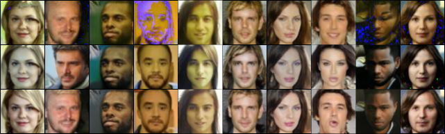
Figure 2: Typical examples of images generated with $100$ iterations and $\eta=0$. For three different models trained with different noise distributions - (i) First row - single Gaussian noise (ii) Second row - Mixture of Gaussian noise, (iii) Third row - Gamma noise. All models start from the same noise instance.

5 Limitations

While we were able to add two new distributions to the toolbox of diffusion methods, we were not able to provide a complete characterization of all suitable distributions. This effort is left as future work. Additionally, our work suggests that the Gaussian noise should be replaced. However, we still need to identify the conditions in which each of the distributions would outperform the others.

6 Conclusions

We present two novel diffusion models. The first employs a mixture of two Gaussians and the second the Gamma noise distribution. A key enabler for using these distributions is a closed form formulation (Eq. 18 and Eq. 21) of the multi-step noising process, which allows for efficient training. These two models improve the quality of the generated image and audio as well as the speed of generation in comparison to conventional Gaussian-based diffusion processes.

7 Acknowledgments

This project has received funding from the European Research Council (ERC) under the European Unions Horizon 2020 research and innovation programme (grant ERC CoG 725974). The contribution of Eliya Nachmani is part of a Ph.D. thesis research conducted at Tel Aviv University.

References

- [1] Mikołaj Bińkowski, Jeff Donahue, Sander Dieleman, Aidan Clark, Erich Elsen, Norman Casagrande, Luis C Cobo, and Karen Simonyan. High fidelity speech synthesis with adversarial networks. arXiv preprint arXiv:1909.11646, 2019.
- [2] Nanxin Chen, Yu Zhang, Heiga Zen, Ron J. Weiss, Mohammad Norouzi, and William Chan. WaveGrad: Estimating gradients for waveform generation. 2020.
- [3] Chris Donahue, Julian McAuley, and Miller Puckette. Adversarial audio synthesis. arXiv preprint arXiv:1802.04208, 2018.
- [4] Ruiqi Gao, Yang Song, Ben Poole, Ying Nian Wu, and Diederik P Kingma. Learning energy-based models by diffusion recovery likelihood. arXiv preprint arXiv:2012.08125, 2020.
- [5] Ian J Goodfellow, Jean Pouget-Abadie, Mehdi Mirza, Bing Xu, David Warde-Farley, Sherjil Ozair, Aaron Courville, and Yoshua Bengio. Generative adversarial networks. arXiv preprint arXiv:1406.2661, 2014.
- [6] Martin Heusel, Hubert Ramsauer, Thomas Unterthiner, Bernhard Nessler, and Sepp Hochreiter. Gans trained by a two time-scale update rule converge to a local nash equilibrium. arXiv preprint arXiv:1706.08500, 2017.
- [7] Jonathan Ho, Ajay Jain, and Pieter Abbeel. Denoising diffusion probabilistic models. arXiv preprint arXiv:2006.11239, 2020.
- [8] Aapo Hyvärinen and Peter Dayan. Estimation of non-normalized statistical models by score matching. Journal of Machine Learning Research, 6(4), 2005.
- [9] Keith Ito and Linda Johnson. The lj speech dataset. https://keithito.com/LJ-Speech-Dataset/, 2017.
- [10] Chenlin Meng Jiaming Song and Stefano Ermon. Denoising diffusion implicit models. https://github.com/ermongroup/ddim, 2020.
- [11] Nal Kalchbrenner, Erich Elsen, Karen Simonyan, Seb Noury, Norman Casagrande, Edward Lockhart, Florian Stimberg, Aaron Oord, Sander Dieleman, and Koray Kavukcuoglu. Efficient neural audio synthesis. In International Conference on Machine Learning, pages 2410–2419. PMLR, 2018.
- [12] Tero Karras, Samuli Laine, Miika Aittala, Janne Hellsten, Jaakko Lehtinen, and Timo Aila. Analyzing and improving the image quality of stylegan. In Proceedings of the IEEE/CVF Conference on Computer Vision and Pattern Recognition, pages 8110–8119, 2020.
- [13] Diederik P Kingma and Prafulla Dhariwal. Glow: Generative flow with invertible 1x1 convolutions. arXiv preprint arXiv:1807.03039, 2018.
- [14] Diederik P Kingma and Max Welling. Auto-encoding variational bayes. arXiv preprint arXiv:1312.6114, 2013.
- [15] Zhifeng Kong, Wei Ping, Jiaji Huang, Kexin Zhao, and Bryan Catanzaro. DiffWave: A versatile diffusion model for audio synthesis. 2020.
- [16] Zhifeng Kong, Wei Ping, Jiaji Huang, Kexin Zhao, and Bryan Catanzaro. Diffwave: A versatile diffusion model for audio synthesis. arXiv preprint arXiv:2009.09761, 2020.
- [17] R. Kubichek. Mel-cepstral distance measure for objective speech quality assessment. In Proceedings of IEEE Pacific Rim Conference on Communications Computers and Signal Processing, volume 1, pages 125–128 vol.1, 1993.
- [18] Lawrence M Leemis and Jacquelyn T McQueston. Univariate distribution relationships. The American Statistician, 62(1):45–53, 2008.
- [19] Qiang Liu, Jason Lee, and Michael Jordan. A kernelized stein discrepancy for goodness-of-fit tests. In International conference on machine learning, pages 276–284. PMLR, 2016.
- [20] Ziwei Liu, Ping Luo, Xiaogang Wang, and Xiaoou Tang. Deep learning face attributes in the wild. In Proceedings of International Conference on Computer Vision (ICCV), December 2015.
- [21] Anton Obukhov, Maximilian Seitzer, Po-Wei Wu, Semen Zhydenko, Jonathan Kyl, and Elvis Yu-Jing Lin. High-fidelity performance metrics for generative models in pytorch, 2020. Version: 0.2.0, DOI: 10.5281/zenodo.3786540.
- [22] Aaron van den Oord, Sander Dieleman, Heiga Zen, Karen Simonyan, Oriol Vinyals, Alex Graves, Nal Kalchbrenner, Andrew Senior, and Koray Kavukcuoglu. Wavenet: A generative model for raw audio. arXiv preprint arXiv:1609.03499, 2016.
- [23] Ali Razavi, Aaron van den Oord, and Oriol Vinyals. Generating diverse high-fidelity images with vq-vae-2. arXiv preprint arXiv:1906.00446, 2019.
- [24] A. W. Rix, J. G. Beerends, M. P. Hollier, and A. P. Hekstra. Perceptual evaluation of speech quality (pesq)-a new method for speech quality assessment of telephone networks and codecs. In 2001 IEEE International Conference on Acoustics, Speech, and Signal Processing. Proceedings (Cat. No.01CH37221), volume 2, pages 749–752 vol.2, 2001.
- [25] Jascha Sohl-Dickstein, Eric Weiss, Niru Maheswaranathan, and Surya Ganguli. Deep unsupervised learning using nonequilibrium thermodynamics. In International Conference on Machine Learning, pages 2256–2265. PMLR, 2015.
- [26] Jiaming Song, Chenlin Meng, and Stefano Ermon. Denoising diffusion implicit models. 2020.
- [27] Yang Song and Stefano Ermon. Generative modeling by estimating gradients of the data distribution. arXiv preprint arXiv:1907.05600, 2019.
- [28] Yang Song, Jascha Sohl-Dickstein, Diederik P Kingma, Abhishek Kumar, Stefano Ermon, and Ben Poole. Score-based generative modeling through stochastic differential equations. arXiv preprint arXiv:2011.13456, 2020.
- [29] C. H. Taal, R. C. Hendriks, R. Heusdens, and J. Jensen. An algorithm for intelligibility prediction of time–frequency weighted noisy speech. IEEE Transactions on Audio, Speech, and Language Processing, 19(7):2125–2136, 2011.
- [30] Arash Vahdat and Jan Kautz. Nvae: A deep hierarchical variational autoencoder. arXiv preprint arXiv:2007.03898, 2020.
- [31] Ivan Vovk. Wavegrad. https://github.com/ivanvovk/WaveGrad, 2020.
- [32] Fisher Yu, Yinda Zhang, Shuran Song, Ari Seff, and Jianxiong Xiao. Lsun: Construction of a large-scale image dataset using deep learning with humans in the loop. arXiv preprint arXiv:1506.03365, 2015.