Global planar dynamics with star nodes: beyond Hilbert’s $16^{th}$ problem

Abstract.

This is a complete study of the dynamics of polynomial planar vector fields whose linear part is a multiple of the identity and whose nonlinear part is a homogeneous polynomial. It extends previous work by other authors that was mainly concerned with the existence and number of limit cycles. The general results are also applied to two classes of examples where the nonlinearities have degrees 2 and 3, for which we provide a complete set of phase portraits.

$A$ Departamento de Matemática Aplicada, Instituto de Matemática e Estatística, Universidade Federal Fluminense,
Rua Professor Marcos Waldemar de Freitas Reis, S/N, Bloco H,
Campus do Gragoatá, CEP 24.210 – 201, São Domingos — Niterói, RJ, Brasil
$B$ Centro de Matemática da Universidade do Porto,
Rua do Campo Alegre 687, 4169-007 Porto, Portugal.
$C$ Faculdade de Economia do Porto,
Rua Dr. Roberto Frias, 4200-464 Porto, Portugal.
$D$ Faculdade de Ciências da Universidade do Porto,
Rua do Campo Alegre 687, 4169-007 Porto, Portugal.

Keywords: Planar autonomous ordinary differential equations; polynomial differential equations; homogeneous nonlinearities; star nodes

AMS Subject Classifications: Primary: 34C05, 37C70; Secondary: 34C37, 37C10

1. Introduction

Global planar dynamics of polynomial vector fields has been of interest for many years. Part of this interest arises from its connection to Hilbert’s $16^{th}$ problem on the number of limit cycles for the dynamics. Because of Hilbert’s $16^{th}$ problem, substantial effort has been devoted to establishing a bound for the number of limit cycles. For some contributions in this direction when the vector field has homogeneous nonlinearities see the work of Boukoucha [4], Bendjeddou et al. [2], Huang et al. [14], Gasull et al. [13], Llibre et al. [16] or Carbonell and Llibre [5], and more recently García-Saldaña et al. [12]. This question has also been approached using bifurcations by, for instance, Benterki and Llibre [3] or [13]. Problems with symmetry appear in Álvarez et al. [1] and Labouriau and Murza [15].

We are, of course, also concerned in establishing an upper bound for the number of limit cycles. However, when no limit cycle exists, we take a different route and address the question of the existence of polycycles and the number of equilibria in them.

We focus on polynomial vector fields with homogeneous nonlinearities, as many before us, but use the existence of invariant lines through the origin to provide information on the global dynamics. We consider vector fields of the form

(1) $$\left\{\begin{array}[]{lcl}\dot{x}&=&\lambda x+Q_{1}(x,y)\\ \mbox{}&\mbox{}&\\ \dot{y}&=&\lambda y+Q_{2}(x,y)\end{array}\right.$$

where $\lambda\neq 0$ and $Q_{i}$, $i=1,2$ are homogeneous non-zero polynomials of the same degree $n>1$. We define $Q=(Q_{1},Q_{2})$ and say it is a homogeneous polynomial of degree $n$. The origin of such a system is an unstable star node (a node with equal and positive eigenvalues) if $\lambda>0$ and a stable star node (a node with equal and negative eigenvalues) if $\lambda<0$.

Using both the dynamics of the vector field at infinity, through its Poincaré compactification, as well as polar coordinates, we describe completely the existence of equilibria at infinity. These occur as equilibria on the boundary of the Poincaré disk for the dynamics of the compactification. We distinguish them from finite equilibria, occurring in the interior of the Poincaré disk, by calling them infinite equilibria. The existence of infinitely many infinite equilibria determines that either there are also infinitely many finite equilibria or the origin is the only finite equilibrium. The case of finitely many infinite equilibria allows for a complete description of the planar dynamics. Each equilibrium at infinity defines an invariant radius with the origin. Other finite equilibria are located on such radii. We are able to provide an upper bound for the number of finite equilibria which improves on Bezout’s Theorem for polynomials of degree strictly greater than 3. We also describe the stability of all equilibria.

The above is a preliminary step for our main contribution to the description of the global planar dynamics with star nodes. This relies on the construction of invariant sectors from the invariant radii. We show that there are only four types of sectors allowed. The number of sectors necessary for the full description of the global dynamics depends on the number of infinite equilibria (whose upper bound we have established previously). Polycycles are present only when one type of sector repeats to cover the plane. A limit cycle exists only when there are no infinite equilibria. It can arise as a generic perturbation of a heteroclinic cycle that collapses through a saddle-node bifurcation. Together with ours, results previously established by Bendjeddou et al. [2], Coll et al. [8], and Gasull et al. [13] completely describe the case when the origin is a global attractor or repellor.

We illustrate our results by fully studying the cases when the nonlinear polynomials are of degree 2 and 3. To this purpose, we build also on previous results of Cima and Llibre [6] and Date [10]. In both cases we provide the complete list of admissible phase portraits for the global dynamics. This article is thus a preliminary step towards the study of the probability of occurrence of a given phase portrait along the lines of Cima et al. [7]. For higher degree the interested reader may apply the same procedure to the classification of Collins [9].

This article is organised as follows: in the next section we provide some background and establish our notation. In Section 3, we describe the equilibria as well as their stability. Section 4 provides a complete description of the global dynamics, including the existence of limit cycles and polycycles. In the final section we present two families of examples when the nonlinear part of (1) is of degree 2 and of degree 3.

2. Preliminary results and notation

We describe the global dynamics for (1) depending on whether the finite degree $n$ is even or odd.

We use the compactification of ${\bf R}^{2}$ in Chapter 5 of Dumortier et al. [11] to describe the dynamics at infinity of (1) and to show that it determines the dynamics in ${\bf R}^{2}$. The beginning of this section is devoted to recalling the Poincaré compactification and establishing some convenient notation that we use throughout.

Let $\mathcal{S}^{2}\subset{\bf R}^{3}$ be the unit sphere and identify ${\bf R}^{2}$ with the plane $\{(x,y,1)\in{\bf R}^{3}:x,y\in{\bf R}\}$. Using coordinates $(z_{1},z_{2},z_{3})$ for ${\bf R}^{3}$, define charts $U_{k}=\{z\in\mathcal{S}^{2}:z_{k}>0\}$ and $V_{k}=\{z\in\mathcal{S}^{2}:z_{k}<0\}$ for $k=1,2,3$. The local maps corresponding to these charts are $\phi_{k}(z)=-\psi_{k}(z)=(z_{m}/z_{k},z_{n}/z_{k})$ for $m<n$ and $m,n\neq k$. Use $(u,v)$ to denote the value of the image under any of the local maps, so that the meaning of $(u,v)$ has to be determined in connection to each local chart. A point with coordinates $(u,v)$, $u\neq 0$ in $U_{i}$ or $V_{i}$ corresponds to the point with coordinates $(\tilde{u},\tilde{v})=\left({1}/{u},{v}/{u}\right)$ in $U_{j}$ or $V_{j}$ with $i\neq j$. The plane ${\bf R}^{2}$ is identified with the open northern hemisphere, the Poincaré disk is defined as its closure. By making $v=0$ in $U_{1}$, $U_{2}$, $V_{1}$, $V_{2}$ we obtain the equator $\mathcal{S}^{1}$ of the sphere, the circle at infinity of the Poincaré disk.

A direct application of the calculations in Dumortier et al. [11] shows that the dynamics of (1) in the Poincaré compactification is given, in the chart $U_{1}$, by:

(2) $$\left\{\begin{array}[]{lcl}\dot{u}&=&F(u)\\ {}&{}\hfil&\\ \dot{v}&=&-\lambda v^{n}-vQ_{1}(1,u)\end{array}\right.\qquad\mbox{where}\qquad F(u)=Q_{2}(1,u)-uQ_{1}(1,u)$$

and in the chart $U_{2}$, by:

(3) $$\left\{\begin{array}[]{lcl}\dot{u}&=&G(u)\\ {}&{}\hfil&\\ \dot{v}&=&-\lambda v^{n}-vQ_{2}(u,1)\end{array}\right.\qquad\mbox{where}\qquad G(u)=Q_{1}(u,1)-uQ_{2}(u,1).$$

The expressions of the Poincaré compactification in the charts $V_{1}$ and $V_{2}$ are obtained from those in the charts $U_{1}$ and $U_{2}$, respectively, by multiplication by $(-1)^{n-1}$.

The dynamics at infinity of (1) is thus given by the restriction of either (2) or (3) to the flow-invariant line $(u,0)$, since the second equation is trivially satisfied for $v=0$. An equilibrium at infinity of (1) is an equilibrium $(u,0)\in\mathcal{S}^{1}$ of either (2) or (3). We refer to it as an infinite equilibrium, by opposition to finite equilibria $(u,v)$, $v\neq 0$.

It is clear that the dynamics of the restriction of either (2) or (3) to the flow-invariant circle at infinity $(u,0)$ does not depend on $\lambda$ and therefore, does not depend on the linear part of (1). Hence, it is equivalent to

$$\left\{\begin{array}[]{lcl}\dot{x}&=&Q_{1}(x,y)\\ \mbox{}&\mbox{}&\\ \dot{y}&=&Q_{2}(x,y)\end{array}\right.$$

In the special case where the polynomials $Q_{1}$ and $Q_{2}$ in (1) have no common factor it was established in [6, Theorem 4.4] that the dynamics at infinity is determined by $(Q_{1},Q_{2})$. In our case the result holds without the common factor assumption.

A useful alternative description of the dynamics can be obtained from considering the representation of (1) in polar coordinates $(x,y)=(r\cos\theta,r\sin\theta)$, $(r,\theta)\in\mathbb{R}^{+}\times\mathcal{S}^{1}$. This is given by

(4) $$\left\{\begin{array}[]{l}\dot{r}=\lambda r+f(\theta)r^{n}\\ \dot{\theta}=g(\theta)r^{n-1}\end{array}\right.$$

where

(5) $$f(\theta)=\cos\theta Q_{1}(\cos\theta,\sin\theta)+\sin\theta Q_{2}(\cos\theta,\sin\theta)$$

and

(6) $$g(\theta)=\cos\theta Q_{2}(\cos\theta,\sin\theta)-\sin\theta Q_{1}(\cos\theta,\sin\theta).$$

Observe that $f(\theta+\pi)=(-1)^{n+1}f(\theta)$ and $g(\theta+\pi)=(-1)^{n+1}g(\theta)$.

We refer to the half-line $\theta=\theta_{0}$, $r>0$ as the radius $\theta=\theta_{0}$ and to the line $\theta=\theta_{0}$, $r\in{\bf R}$ as the diameter $\theta=\theta_{0}$.

Lemma 2.1.

The polynomials $Q_{1}$, $Q_{2}$ have a common linear factor if and only if $f(\theta)$ and $g(\theta)$ vanish simultaneously.

Proof.

Assume $g(\theta_{0})=0$ for some $\theta_{0}$, with $\cos{\theta_{0}}\neq 0$ (otherwise, proceed analogously for $\sin(\theta_{0})\neq 0$). Then, from (6), $g(\theta_{0})=0\Leftrightarrow Q_{2}(\cos{\theta_{0}},\sin{\theta_{0}})=\tan{\theta_{0}}Q_{1}(\cos{\theta_{0}},\sin{\theta_{0}})$. Replacing in (5), we obtain $f(\theta_{0})=0\Leftrightarrow Q_{1}(\cos{\theta_{0}},\sin{\theta_{0}})=0$. Hence, for the same $\theta_{0}$ it is $Q_{1}(\cos{\theta_{0}},\sin{\theta_{0}})=Q_{2}(\cos{\theta_{0}},\sin{\theta_{0}})$ and this is true if and only if the polynomials have a common linear factor. ∎

Note that the components of (1) never have common factors even when $Q_{1}$ and $Q_{2}$ do.

3. Equilibria

This section is concerned with the number and stability of equilibria of (1) in the Poincaré compactification, both finite and infinite. We start with the behaviour at infinity.

Lemma 3.1.

The dynamics of the vector field (4) at the equator of the Poincaré disk is described by $\dot{\theta}=g(\theta)$.

Proof.

Let $u=\tan{\theta}$ in $U_{1}$ and $u=\cot{\theta}$ in $U_{2}$, respectively. Then using (2) and (3) it follows that $\dot{\theta}=\sqrt{2^{1-n}}g(\theta)$. Hence, the vector field at the equator of the Poincaré disk is topologically equivalent to $\dot{\theta}=g(\theta)$. ∎

One special case where $Q_{1}$ and $Q_{2}$ have a common factor is described in the next result. It also implies that generically there will be either no equilibria at infinity or a finite number of them.

Lemma 3.2.

There are infinitely many equilibria of (1) at infinity if and only if $yQ_{1}(x,y)=xQ_{2}(x,y)$. Moreover, in this case either there are also infinitely many finite equilibria or the only finite equilibrium is the origin.

Proof.

Equilibria at infinity are points $(u,0)$ that satisfy either $F(u)=0$ or $G(u)=0$. Since both $F(u)$ and $G(u)$ are polynomials, in order to have infinitely many roots we must have either $F(u)\equiv 0$ or $G(u)\equiv 0$. Direct substitution in the expressions for $F(u)$ and $G(u)$ shows that if $yQ_{1}(x,y)=xQ_{2}(x,y)$ then $F(u)=G(u)\equiv 0$. To show the converse, write

$$Q_{1}(x,y)=\sum_{k=0}^{n}c_{k}x^{n-k}y^{k}\quad\mbox{and}\quad Q_{2}(x,y)=\sum_{k=0}^{n}d_{k}x^{n-k}y^{k}$$

to obtain

(7) $$F(u)=\sum_{k=0}^{n}d_{k}u^{k}-\sum_{k=1}^{n+1}c_{k-1}u^{k}\qquad\qquad G(u)=\sum_{\ell=0}^{n}c_{n-\ell}u^{\ell}-\sum_{\ell=1}^{n+1}d_{n-\ell+1}u^{\ell}.$$

Hence, $F(u)\equiv 0$ if and only if

$$c_{n}=0=d_{0}\quad\mbox{and}\quad d_{k}=c_{k-1}\quad k=1,\ldots,n.$$

Exactly the same conditions hold for $G(u)\equiv 0$.

Therefore, we can write $Q_{1}(x,y)=xp(x,y)$ and $Q_{2}(x,y)=yp(x,y)$ where

$$p(x,y)=\sum_{k=0}^{n-1}c_{k}x^{n-k-1}y^{k}$$

is a homogeneous polynomial. That is, $yQ_{1}(x,y)=xQ_{2}(x,y)$. In this case, finite equilibria of (1) satisfy:

$$\dot{x}=0\quad\Leftrightarrow\quad x=0\mbox{ or }p(x,y)=-\lambda\qquad\mbox{and}\qquad\dot{y}=0\quad\Leftrightarrow\quad y=0\mbox{ or }p(x,y)=-\lambda.$$

Since the equation $p(x,y)=-\lambda\neq 0$ has either infinitely many solutions or none, the result follows. ∎

The next results provide the possible configuration of finite equilibria. They are similar in nature to [5, Lemma 3.1] but describe cases not covered there.

Lemma 3.3.

If $n$ is even then there is at least one pair of infinite equilibria of (1).

Proof.

Using (7), we see that the degree of $F$ is either $n+1$, in which case there is at least one infinite equilibrium, or lower. If the degree of $F$ is less than $n+1$ then $c_{n}=0$. If $c_{n}=0$ then $G(0)=0$ and again there is an infinite equilibrium. When $n$ is even, since $g(\theta)=g(\theta+\pi)$, the infinite equilibria occur in pairs. ∎

Proposition 3.4.

There is an infinite equilibrium of (1) on the radius $\theta=\theta_{0}$ if and only if $g(\theta_{0})=0$, and in this case

1. the diameter $\theta=\theta_{0}$ is flow-invariant;

2. if $\lambda f(\theta_{0})<0$ there is a unique finite equilibrium on the radius $\theta=\theta_{0}$;

3. if $\lambda f(\theta_{0})\geq 0$ there are no finite equilibria on the radius $\theta=\theta_{0}$.

Proof.

The existence of the infinite equilibrium follows from Lemma 3.1 and the invariance of the diameter is immediate from (4). Finite equilibria $(r_{0},\theta_{0})$ with $r_{0}>0$ satisfy

$$\left.\dot{r}\right|_{\theta_{0}}=\lambda r_{0}+f(\theta_{0})r_{0}^{n}=0.$$

Hence, $0<r_{0}^{n-1}=-\lambda/f(\theta_{0})$, establishing (b) and (c). ∎

From $f(\theta+\pi)=(-1)^{n+1}f(\theta)$ and $g(\theta+\pi)=(-1)^{n+1}g(\theta)$, it follows that

• if $n$ is even, the inequalities in (b) and (c) are reversed for $\theta_{0}+\pi$;

• if $n$ is odd (b) and (c) also hold for $\theta_{0}+\pi$.

The following corollary is then immediate.

Corollary 3.5.

Let there be $\theta_{0}$ such that $g(\theta_{0})=0$ in (6). Then

1. there is an infinite equilibrium on the radius $\theta=\theta_{0}+\pi$;

2. if $n$ is even then

   1. if $f(\theta_{0})\neq 0$ then one of the radii $\theta=\theta_{0}$ and $\theta=\theta_{0}+\pi$ contains a single finite equilibrium and there are no finite equilibria on other radius;

   2. if $f(\theta_{0})=0$ there are no finite equilibria on any of the radii $\theta=\theta_{0}$ and $\theta=\theta_{0}+\pi$;

3. if $n$ is odd then

   1. if $\lambda f(\theta_{0})<0$ there exists a unique finite equilibrium on each one of the radii $\theta=\theta_{0}$ and $\theta=\theta_{0}+\pi$;

   2. if $\lambda f(\theta_{0})\geq 0$ there are no finite equilibria on any of the radii $\theta=\theta_{0}$ and $\theta=\theta_{0}+\pi$.

Thus, for each finite equilibrium there is a corresponding equilibrium at infinity. The converse may not be true: the set of infinite equilibria may even be a continuum, with only one finite equilibrium, as in Lemma 3.2.

By Bezout’s Theorem, if (1) has finitely many equilibria, then they are at most $n^{2}$. The next result shows that this estimate may be improved for $n>3$ (the estimate is the same if $n\leq 3$).

Theorem 3.6.

Assume that $Q$ in (1) is a homogeneous polynomial vector field of degree $n$. Assume that (1) has finitely many infinite equilibria, then

1. for all $n>1$ there are at most $2(n+1)$ infinite equilibria.

2. if $n$ is odd then the number of finite equilibria away from the origin is at most $2(n+1)$;

3. if $n$ is even then the number of finite equilibria away from the origin is at most $n+1$;

Proof.

We start by estimating the number of infinite equilibria. As in the proof of Lemma 3.2 there are infinitely many equilibria at infinity if and only if $F(u)\equiv 0$ or $G(u)\equiv 0$, we suppose this is not the case. As $F(u)$ is a polynomial of degree at most $n+1$ the maximum number of infinite equilibria in the chart $U_{1}$ is $n+1$. Since the same holds in the chart $V_{1}$, the maximum number of infinite equilibria arising from the zeros of $F$ is $2(n+1)$, establishing (a). The zeros of $G(u)$ yield the same infinite equilibria except for $u=0$, which does not belong to $U_{1}\cup V_{1}$. If $G(0)=0$, by (7), we have $c_{n}=0$ and an additional infinite equilibrium in each of the charts $U_{2}$ and $V_{2}$. However, when $c_{n}=0$ the degree of $F$ is $n$, rather than $n+1$, producing the same maximum number of $2(n+1)$.

Equilibria at infinity correspond to roots of $g(\theta)=0$. If the infinite equilibrium on the radius $\theta=\theta_{0}$ lies in the neighbourhood $U_{i}$ then the equilibrium on the radius $\theta=\theta_{0}+\pi$ lies in $V_{i}$.

If $n$ is odd then Proposition 3.4 shows that for each one of the infinite equilibria on the radii $\theta=\theta_{0}$ and $\theta=\theta_{0}+\pi$, there may be at most one finite equilibrium point on each one of these radii. Therefore the total number of finite equilibria is at most $2(n+1)$, as in (b).

For even $n$, by Proposition 3.4 only one of the radii $\theta=\theta_{0}$ and $\theta=\theta_{0}+\pi$ may contain a finite equilibrium, hence the maximum number is $n+1$, establishing (c). ∎

Corollary 3.7.

Let $Q$ be a homogeneous polynomial vector field of degree $2p+1$ and suppose (1) has finitely many equilibria at infinity. If in the restriction to the circle at infinity all equilibria are either attracting or repelling then the number of equilibria at infinity is a multiple of 4.

In particular Corollary 3.7 implies that when all infinite equilibria are hyperbolic their total number is a multiple of 4.

Proof.

As in the proof of Theorem 3.6 we count the equilibria in the chart $U_{1}$ ($V_{1}$, respectively) in the restriction to the circle at infinity. Equilibria at infinity that are either attracting or repelling correspond to roots where $F(u)$ (respectively $G(u)$) changes sign, hence they are roots of odd multiplicity. If $F(u)$ has degree $2p+2$ then there must be an even number of these roots. In this case $G(0)\neq 0$ and these are all the equilibria in the charts $U_{1}$ and $V_{1}$. If the degree of $F(u)$ is $2p+1$ then the number of its roots is odd and $G(0)=0$, so again the total number of equilibria in the charts $U_{1}$ and $V_{1}$ is even. Adding the same number of roots in the charts $U_{2}$ and $V_{2}$ establishes the result. ∎

The next result concerns the stability of the equilibria of (1). In the case of infinite equilibria it repeats results in Proposition 4.1 (c) in [6], which we include here for ease of reference.

Proposition 3.8.

If (1) has finitely many equilibria at infinity, then:

1. the linearisation of (2) and (3) at any (finite or infinite) equilibrium has real eigenvalues, in particular, all equilibria are topological nodes (attractors or repellors), saddles or saddle-nodes;

2. the infinite equilibrium on the radius $\theta=\theta_{0}$ is radially attracting if either $f(\theta_{0})>0$ or $f(\theta_{0})=0$ and $\lambda>0$, radially repelling otherwise;

3. the stability in the angular direction of an equilibrium (finite or infinite) on the radius $\theta=\theta_{0}$ is determined by the sign of $g^{\prime}(\theta_{0})$, and in the radial direction, for finite equilibria, by the sign of $-\lambda$;

4. an equilibrium $(u_{0},v_{0})$ (finite or infinite) in the chart $U_{1}$ (respectively $U_{2}$) is a saddle-node if and only if $u_{0}$ is a root of even multiplicity of $F(u)$ in (2) (respectively $G(u)$ in (3)).

Proof.

In both (2) and (3) the expression for $\dot{u}$ does not depend on $v$, hence the Jacobian matrix is triangular and the eigenvalues are real, proving (a).

Using polar coordinates (4), at a finite equilibrium $(r_{0},\theta_{0})$ we have $r_{0}^{n-1}=\lambda/f(\theta_{0})<0$, and the Jacobian matrix of (4) is the triangular matrix

(8) $$J(r_{0},\theta_{0})=\left(\begin{array}[]{cc}-\lambda(n-1)&f^{\prime}(\theta_{0})r_{0}^{n}\\ 0&g^{\prime}(\theta_{0})\left(\frac{-\lambda}{f(\theta_{0})}\right)\\ \end{array}\right).$$

Hence, the radial direction is an eigenspace corresponding to the non-zero eigenvalue $-\lambda(n-1)$, whose sign is the opposite of that of $\lambda$. The stability of a finite equilibrium $(r_{0},\theta_{0})$ in the angular direction depends on the sign of $g^{\prime}(\theta_{0})$ since $-\lambda/f(\theta_{0})>0$. It follows from Lemma 3.1 that this stability coincides with that at infinity, proving (c).

The dynamics near the equator of the Poincaré disk can be described by making the change of coordinates $R=r^{1-n}$ in (4) and analysing (9) near $R=0$. We obtain

(9) $$\dot{R}=-(n-1)[\lambda R+f(\theta)].$$

If $f(\theta_{0})\neq 0$ then for small $R$ the sign of $\dot{R}$ is the same as the sign of $-f(\theta_{0})$. When $f(\theta_{0})=0$ then $\dot{R}$ has the sign of $-\lambda$ for small $R>0$, proving (b). Note that for $f(\theta)=0$ the infinite equilibrium is not hyperbolic.

For an infinite equilibrium, statement (d) is proved in [6, Proposition 4.1 (c)]. At a finite equilibrium the radial eigenvalue of $J(r_{0},\theta_{0})$ is never zero, and (d) holds for the angular direction, by (c). ∎

4. Invariant regions and polycycles

The aim of this section is to describe how the dynamics of (1) at infinity constrains the geometry of flow-invariant sets other than equilibria. We start by the cases when the dynamics is simpler. The next result is a synthesis of Theorem 2 in [2] and Theorem A in [8], as well as Theorems 2 and 3 in [13], we include it here for ease of reference.

Theorem 4.1.

For (1) with $n>1$ and $\lambda\neq 0$:

1. there is at most one non-constant periodic solution and its trajectory surrounds the origin;

2. if $n$ is even then there are no periodic trajectories surrounding the origin;

3. if $n$ is odd and $g(\theta)=0$ for some $\theta\in[0,2\pi)$ then there are no periodic trajectories surrounding the origin;

4. if $n$ is odd and $g(\theta)\neq 0$ for all $\theta\in[0,2\pi)$ then the origin is the only equilibrium of (1) and there is a limit cycle surrounding the origin if and only if $\lambda\int_{0}^{2\pi}\frac{f(\theta)}{|g(\theta)|}d\theta<0$;

5. if there is a limit cycle it is hyperbolic.

From this result and Proposition 3.4 we obtain a description of the cases of trivial dynamics.

Corollary 4.2.

The origin is a globally attracting ($\lambda<0$) or repelling ($\lambda>0$) equilibrium point of (1) if and only if one of the following conditions holds:

1. $n$ is even and $f(\theta)=0$ whenever $g(\theta)=0$;

2. $n$ is odd and $\lambda f(\theta)\geq 0$ whenever $g(\theta)=0$;

3. $n$ is odd with $g(\theta)\neq 0$ for all $\theta\in[0,2\pi)$ and $\lambda\int_{0}^{2\pi}\frac{f(\theta)}{|g(\theta)|}d\theta\geq 0$;

Proof.

By Proposition 3.4 the conditions on $f(\theta)$ and $g(\theta)$ of (a)–(c) are equivalent to the origin being the only finite equilibrium of (1). Hence the conditions are necessary.

To show they are sufficient we establish the absence of non-trivial periodic trajectories. If $n$ is odd this is guaranteed by condition (c). This is also true if $n$ is even by Theorem 4.1 (b) and Lemma 3.3, establishing condition (a).

If $n$ is odd and $g(\theta_{0})=0$ for some $\theta_{0}$ then (c) of Theorem 4.1 implies the sufficiency of condition (b). ∎

In the remainder of this section we discuss the dynamics of (1) when $g(\theta_{0})=0$ for some $\theta_{0}\in[0,2\pi)$. This condition, by Proposition 3.4, implies the existence of two infinite equilibria. It also implies the flow-invariance of the diameter $\theta=\theta_{0}$. Let $\alpha_{1}$ and $\alpha_{2}$ be two consecutive infinite equilibria corresponding to two consecutive zeros of $g(\theta)$, $\theta_{1}$ and $\theta_{2}$. These define a flow-invariant set given in polar coordinates by $\left\{(r,\theta)\ :\ r\in{\bf R},\ \theta_{1}\leq\theta\leq\theta_{2}\right\}$, with $0<\theta_{2}-\theta_{1}\leq\pi$. We refer to this flow-invariant set as a flow-invariant cone (or simply a cone) and to its non-negative ($r\geq 0$) component as a half-cone.

Therefore, to equilibria at infinity there corresponds a division of the plane in invariant half-cones between consecutive invariant radii. An upper bound for the number of half-cones can be obtained from Theorem 3.6.

Corollary 4.3.

If the homogeneous polynomial $Q$ has degree $n$ then there are at most $n+1$ cones that are invariant under the flow of (1). If $n$ is even there is at least one pair of invariant half-cones.

Proof.

Each pair of infinite equilibria, satisfying $g(\theta_{0})=0=g(\theta_{0}+\pi)$ determines a flow-invariant diameter. From the proof of Theorem 3.6 it follows that there are at most $n+1$ such pairs, independently of the parity of the degree $n$. If $n$ is even then by Proposition 3.4 there is at least one pair of infinite equilibria, giving rise to one pair of invariant half-cones. ∎

An infinite equilibrium $\alpha$ and its associated invariant radius determine two sectors in a neighbourhood in the half-plane $v\geq 0$. Denote by $P^{-}$ a repelling parabolic sector, $P^{+}$ an attracting parabolic sector, $H^{-}$ a radially repelling hyperbolic sector and $H^{+}$ a radially attracting hyperbolic sector. We will show below that this classification of sectors completely determines the dynamics of (1) on the invariant cones.

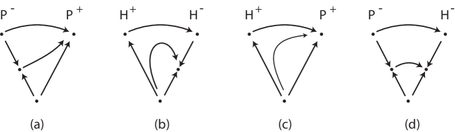
Figure 1. Dynamics in invariant half-cones in Theorem 4.4 for $\lambda>0$. In case (d) there is a robust connection between two finite equilibria.

Theorem 4.4.

The dynamics near infinite equilibria of the vector field (1) determines its global dynamics on the plane.

For a trajectory at infinity connecting two consecutive infinite equilibria $\alpha_{1}$ and $\alpha_{2}$ the dynamics in the half-cone $C$ determined by them is described in Figures 1 and 2, where the possible pairs of sectors at $\alpha_{1}$ and $\alpha_{2}$ are, respectively:

1. $P^{-}$ and $P^{+}$;

2. $H^{+}$ and $H^{-}$;

3. $H^{+}$ and $P^{+}$;

4. $P^{-}$ and $H^{-}$.

Proof.

We start by establishing the list of possible sectors in $C$. Since the infinite equilibria are consecutive, the flow at infinity goes from one of the infinite equilibria to the other. Then, if the sectors are of the same type, $H$ or $P$, they cannot have the same sign. If the sectors are of different types then, of course, one is parabolic. If it is $P^{-}$ then the other sector, which is hyperbolic, is attracting in the angular component and must therefore be radially repelling. That is, it is $H^{-}$. Analogously, if the parabolic sector is $P^{+}$ then the hyperbolic sector is repelling in the angular component. It must therefore be radially attracting, that is, it is $H^{+}$.

Assume that $\lambda>0$ so that the origin is repelling. Because of Proposition 3.4, one is the maximum number of finite equilibria on the radius $\theta=\theta_{i}$ corresponding to $\alpha_{i}$, $i=1,2$. We have that

• a radially repelling sector exists at $\alpha_{i}$ if and only if exactly one finite equilibrium exists on the radius $\theta=\theta_{i}$.

• a radially attracting sector exists at $\alpha_{i}$ if and only if there are no finite equilibria on the radius $\theta=\theta_{i}$.

Since to a finite equilibrium there corresponds an infinite one, and because $\alpha_{1}$ and $\alpha_{2}$ are consecutive infinite equilibria, it follows that there are no finite equilibria in the interior of $C$.

The admissible dynamics are depicted in Figure 1.

For $\lambda<0$ the origin is attracting and the dynamics in $C$ may be obtained by changing time as $s=-t$. The phase portraits are depicted in Figure 2. ∎

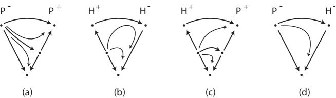
Figure 2. Dynamics in invariant half-cones in Theorem 4.4 for $\lambda<0$. In case (a) the stable manifold of the finite equilibrium splits the half-cone in two basins of attraction. In case (c) there is a robust connection between two finite equilibria. In the remaining cases the origin is a global attractor for the interior of the half-cone.

A polycycle is a flow-invariant simple connected curve in the plane containing at least one equilibrium point and not going through the origin. In the special case when all the trajectories that are not equilibria have the same orientation it is called a heteroclinic cycle.

When one sector is parabolic and the other hyperbolic a finite equilibrium may exist in each radius. If these exist, their radial stability is opposite to that of the origin. Thus the connection between these two finite equilibria is robust as it is either of saddle-sink ($\lambda>0$) or saddle-source ($\lambda<0$) type. See Figures 1 (d) and 2 (c). Note that for a polycycle to exist, all sectors must be alternatingly $H^{-}$ and $P^{-}$. The next results provide more detail concerning polyclycles and heteroclinic cycles.

Proposition 4.5.

The dynamics of (1) exhibits a polycycle if and only if $n$ is odd, there is at least one pair of infinite equilibria and $\lambda f(\theta)<0$ whenever $g(\theta)=0$. Moreover, the polycycle is globally attracting (respectively repelling) if $\lambda>0$ (respectively $\lambda<0$).

Proof.

If $n$ is odd and $\lambda f(\theta)<0$ when $g(\theta)=0$ it follows by Proposition 3.4 that each invariant radius contains a finite equilibrium. On each invariant half-cone one of the sectors is $P^{s}$ and the other is $H^{s}$ where $s$ is the sign of $-\lambda$. By Theorem 4.4 there is a trajectory in the half-cone connecting the two finite equilibria, forming a polycycle. Its dynamics in the radial direction is given by the sign of $-\lambda$. Thus, the polycycle is globally attracting (respectively reppeling) if $\lambda>0$ (respectively $\lambda<0$).

Conversely, if $n$ is even, then for each $\theta_{0}$ such that $g(\theta_{0})=0$, by Proposition 3.4, there is always a radius where there are no finite equilibria. Hence there is a pair of consecutive finite equilibria for which there is no connecting trajectory, as it would have to cross an invariant radius, and there is no polycycle.

The same argument shows that if $n$ is odd and there is a polycycle, then there must be a finite equilibrium on each invariant radius. Proposition 3.4 implies that $\lambda f(\theta)<0$ whenever $g(\theta)=0$. ∎

Another way of stating Proposition 4.5 is that any (finite) polycycle is a copy of the polycycle at infinity, with the radial stability inverted. All the connections of a polycycle for (1) are robust, by (c) and (d) of Theorem 4.4.

Corollary 4.6.

A polycycle of (1) is a heteroclinic cycle if and only if all infinite equilibria are local minima or local maxima of $g$.

Proof.

In a heteroclinic cycle all the equilibria must be connected by trajectories with the same orientation. All the equilibria must be saddle-nodes. Therefore the sign of $g(\theta)$ must be always the same. ∎

In parametrised systems a limit cycle may be created through a saddle-node bifurcation of the equilibria in a heteroclinic cycle. The next result shows that indeed this happens within the class we are studying.

Proposition 4.7.

A 1-parameter perturbation of a heteroclinic cycle for (1) creates a limit cycle.

Proof.

Let $Q_{\varepsilon}(x,y)=\left(Q_{1}(x,y)+\varepsilon P_{1}(x,y),Q_{2}(x,y)+\varepsilon P_{2}(x,y)\right)$ be homogeneous of degree $n$ with $(P_{1}(x,y),P_{2}(x,y))=(-y^{n},x^{n})$. Define $f_{\varepsilon}(\theta)$ and $g_{\varepsilon}(\theta)$ as in (5) and (6), respectively. We have

$$f_{\varepsilon}(\theta) = f(\theta)+\varepsilon\sin\theta\cos\theta(\cos^{n-1}\theta-\sin^{n-1}\theta)$$

$$g_{\varepsilon}(\theta) = g(\theta)+\varepsilon(\cos^{n+1}\theta+\sin^{n+1}\theta).$$

Assume that a heteroclinic cycle exists for the dynamics of (1) when $\varepsilon=0$. By Proposition 4.5 and Corollary 4.6 it must be that the degree of $Q$ is odd, say $n=2m+1$, and $g(\theta)$ has constant sign. Without loss of generality, we assume in this proof that $g(\theta)\geq 0$ for all $\theta$ and that $\lambda>0$, the other cases being analogous. Hence, we also have $f(\theta)<0$ when $g(\theta)=0$.

Note that when $n=2m+1$, for $\varepsilon>0$ we have $g_{\varepsilon}(\theta)>0$ for all $\theta$. Hence, the vector field defined by $Q_{\varepsilon}$ has no infinite equilibria and only the origin is a finite equilibrium. The proof is completed by showing that

(10) $$\int_{0}^{2\pi}\dfrac{f_{\varepsilon}(\theta)}{|g_{\varepsilon}(\theta)|}d\theta<0.$$

Then the hypotheses of Theorem 4.1 (d) are satisfied and for small $\varepsilon>0$ a limit cycle exists. Choose $\varepsilon>0$ small enough so that $f_{\varepsilon}(\theta)<0$ for $\theta$ in intervals containing the $\theta_{i}$ where $g(\theta_{i})=0$. When $\varepsilon\to 0$ we have $g_{\varepsilon}(\theta_{i})\to 0$. Since $\lim_{\varepsilon\to 0}1/{g_{\varepsilon}(\theta_{i})}=+\infty$, the contribution of these intervals to the value of the integral in (10) increases when $\varepsilon$ decreases and the integral is negative for small $\varepsilon>0$. ∎

When (1) has only one pair of infinite equilibria the saddle-node bifurcation described in Proposition 4.7 holds for an open set of homogeneous vector fields near $Q$. This is clearly not true if there is more than one pair of equilibria, since the collapse of the saddle-nodes may not be simultaneous for a generic 1-parameter perturbation.

5. Examples

The results of Sections 3 and 4 are applied here to obtain phase portraits of (1) for nonlinearities of degrees 2 and 3. The dynamics of (1) at infinity depends only on the nonlinear part and by Theorem 4.4 it determines the global dynamics, except when there are no infinite equilibria.

A linear change of coordinates and a time rescaling that preserves orientation transforms the equation $\dot{X}=\lambda X+Q(X)$, with $\lambda\neq 0$, where $X=(x,y)$ and $Q$ is a non-zero homogeneous vector field, into $\dot{X}=\tilde{\lambda}X+\beta{\mathcal{Q}}(X)$ with $\beta=\pm 1$, where $\tilde{\lambda}$ has the same sign as $\lambda$ and ${\mathcal{Q}}$ is a homogeneous polynomial of the same degree as $Q$. This is true because the linear part $\lambda X$ of the equation commutes with every linear map of ${\bf R}^{2}$.

Thus, we can apply the results of Date [10] and of Cima and Llibre [6] on the classification of homogeneous polynomial vector fields of degrees 2 and 3, under linear changes of coordinates and a rescaling of time. Given a homogeneous vector field $Q=(Q_{1},Q_{2})$ on the plane, let ${\mathcal{F}}(x,y)=xQ_{2}(x,y)-yQ_{1}(x,y)$. We have established in Lemma 3.1 that $g(\theta)={\mathcal{F}}(\cos\theta,\sin\theta)$ determines the dynamics of (1) at infinity.

5.1. Example: nonlinearities of degree 2

Homogeneous cubic forms ${\mathcal{F}}(x,y)$ have been classified in [10] and [6]. In order to apply these classifications we compute in the next result the general form of the vector fields of the form (1), with nonlinearities of degree 2, that share the same expression for ${\mathcal{F}}$:

Lemma 5.1.

Let $Q=(Q_{1},Q_{2})$ be a homogeneous quadratic vector field on the plane defining (1). If ${\mathcal{F}}(x,y)=xQ_{2}(x,y)-yQ_{1}(x,y)=a_{0}x^{3}+a_{1}x^{2}y+a_{2}xy^{2}+a_{3}y^{3}$, then there exist $q_{1},q_{2}\in{\bf R}$ such that (1) becomes:

$$\left\{\begin{array}[]{lcl}\dot{x}&=&\lambda x+-a_{0}x^{2}+(q_{1}-a_{1})xy+q_{2}y^{2}\\ \dot{y}&=&\lambda y+q_{1}x^{2}+(q_{2}+a_{2})xy+a_{3}y^{2}\end{array}\right.$$

The next result recovers [10] with the normal forms for ${\mathcal{F}}$ from Theorem 1.4 in [6]. Here $\dot{X}=\tilde{\lambda}X-{\mathcal{Q}}(X)$ is mapped into $\dot{X}=\tilde{\lambda}X+{\mathcal{Q}}(X)$ by a rotation of $\pi$ around the origin, hence we do not need to add $\beta=\pm 1$ to the canonical forms.

Proposition 5.2.

For each homogeneous quadratic vector field $Q=(Q_{1},Q_{2})$ defining (1) there exists a linear change of coordinates and an orientation preserving reparametrisation of time that transforms (1) into only one of the following canonical forms, where $\tilde{\lambda}$ and $\lambda$ have the same sign:

1. $\left\{\begin{array}[]{lcl}\dot{x}&=&\tilde{\lambda}x-x^{2}+q_{1}xy+q_{2}y^{2}\\ \dot{y}&=&\tilde{\lambda}y+q_{1}x^{2}+q_{2}xy+y^{2}\end{array}\right.$     ${\mathcal{F}}(x,y)=x^{3}+y^{3}$
   

2. $\left\{\begin{array}[]{lcl}\dot{x}&=&\tilde{\lambda}x-x^{2}+q_{1}xy+q_{2}y^{2}\\ \dot{y}&=&\tilde{\lambda}y+q_{1}x^{2}+(q_{2}-3)xy\end{array}\right.$     ${\mathcal{F}}(x,y)=x(x^{2}-3y^{2})$
   

3. $\left\{\begin{array}[]{lcl}\dot{x}&=&\tilde{\lambda}x+(q_{1}-3)xy+q_{2}y^{2}\\ \dot{y}&=&\tilde{\lambda}y+q_{1}x^{2}+q_{2}xy\end{array}\right.$     ${\mathcal{F}}(x,y)=3x^{2}y$
   

4. $\left\{\begin{array}[]{lcl}\dot{x}&=&\tilde{\lambda}x-x^{2}+q_{1}xy+q_{2}y^{2}\\ \dot{y}&=&\tilde{\lambda}y+q_{1}x^{2}+q_{2}xy\end{array}\right.$     ${\mathcal{F}}(x,y)=x^{3}$
   

5. $\left\{\begin{array}[]{lcl}\dot{x}&=&\tilde{\lambda}x+q_{1}xy+q_{2}y^{2}\\ \dot{y}&=&\tilde{\lambda}y+q_{1}x^{2}+q_{2}xy\end{array}\right.$     ${\mathcal{F}}(x,y)=0$
   

The phase portraits for these canonical forms may now be obtained using Proposition 3.4, its corollary and Theorem 4.4. They are shown in Figures 3, 4 and 5. Calculations are given in Appendix A.

$q_{2}-q_{1}<1$

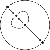
$q_{2}-q_{1}>1$

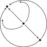
$q_{2}-q_{1}=1$

Figure 3. Phase portraits on the Poincaré disk for normal form (i) in Proposition 5.2 with $\lambda>0$.

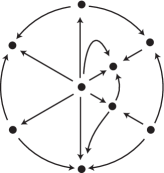
$q_{2}<3-\sqrt{3}q_{1}$

and $q_{2}\leq 3+\sqrt{3}q_{1}$

or

$q_{2}<3-\sqrt{3}q_{1}$

and $q_{2}\leq 3+\sqrt{3}q_{1}$

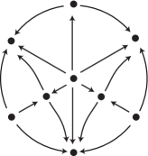
$q_{2}\geq 3-\sqrt{3}q_{1}$

and

$q_{2}\leq 3+\sqrt{3}q_{1}$

$q_{2}<3-\sqrt{3}q_{1}$

and

$q_{2}>3+\sqrt{3}q_{1}$

Figure 4. Phase portraits on the Poincaré disk for normal form (ii) in Proposition 5.2 with $\lambda>0$.

normal form (iii)

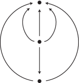
normal form (iv)

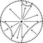
normal form (v)

$q_{1}q_{2}\neq 0$

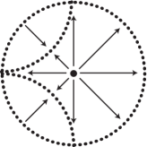
normal form (v)

$q_{1}q_{2}=0$

and $q_{1}+q_{2}\neq 0$.

Figure 5. Phase portraits on the Poincaré disk for normal forms (iii), (iv) and (v) in Proposition 5.2 with $\lambda>0$. The dotted lines for normal form (v) are curves of equilibria, both finite and infinite.

5.2. Example: nonlinearities of degree 3

Cima and Llibre in [6] classify homogeneous binary forms ${\mathcal{F}}(x,y)$ of degree 4 along with homogeneous polynomial vector fields of degree 3, under linear changes of coordinates and a rescaling of time. We use this classification to obtain the dynamics at infinity as a starting point for the following list of canonical forms of homogeneous cubic vector field $Q=(Q_{1},Q_{2})$ defining (1).

Proposition 5.3.

For each non-zero homogeneous cubic vector field $Q=(Q_{1},Q_{2})$ defining (1) there exists a linear change of coordinates and an orientation preserving reparametrisation of time that transforms (1) into only one of the following canonical forms, where $\tilde{\lambda}$ and $\lambda$ have the same sign:

1. $\left\{\begin{array}[]{lcl}\dot{x}&=&\tilde{\lambda}x+\beta\left[x(p_{1}x^{2}+p_{3}y^{2})+y((p_{2}-3\mu)x^{2}-y^{2})\right]\\ \dot{y}&=&\tilde{\lambda}y+\beta\left[y(p_{1}x^{2}+p_{3}y^{2})+x(x^{2}+(p_{2}+3\mu)y^{2})\right]\end{array}\right.$  with $\mu<-\frac{1}{3}$, $\beta=\pm 1$.

2. $\left\{\begin{array}[]{lcl}\dot{x}&=&\tilde{\lambda}x+x(p_{1}x^{2}+p_{3}y^{2})+y((p_{2}-3\alpha\mu)x^{2}-\alpha y^{2})\\ \dot{y}&=&\tilde{\lambda}y+y(p_{1}x^{2}+p_{3}y^{2})+x(\alpha x^{2}+(p_{2}+3\alpha\mu)y^{2})\end{array}\right.$ with $\begin{array}[]{ll}\alpha=\pm 1&\\ \mu>-\frac{1}{3}&\mu\neq\frac{1}{3}\end{array}$

3. $\left\{\begin{array}[]{lcl}\dot{x}&=&\tilde{\lambda}x+\beta\left[x(p_{1}x^{2}+p_{3}y^{2})+y((p_{2}-3\mu)x^{2}+y^{2})\right]\\ \dot{y}&=&\tilde{\lambda}y+\beta\left[y(p_{1}x^{2}+p_{3}y^{2})+x(x^{2}+(p_{2}+3\mu)y^{2})\right]\end{array}\right.$ with $\beta=\pm 1$.

4. $\left\{\begin{array}[]{lcl}\dot{x}&=&\tilde{\lambda}x+x(p_{1}x^{2}+p_{3}y^{2})+y((p_{2}-3\alpha)x^{2}-\alpha y^{2})\\ \dot{y}&=&\tilde{\lambda}y+y(p_{1}x^{2}+p_{3}y^{2})+x((p_{2}+3\alpha)y^{2})\end{array}\right.$ with $\alpha=\pm 1$.

5. $\left\{\begin{array}[]{lcl}\dot{x}&=&\tilde{\lambda}x+x(p_{1}x^{2}+p_{3}y^{2})+y((p_{2}-3\alpha)x^{2}+\alpha y^{2})\\ \dot{y}&=&\tilde{\lambda}y+y(p_{1}x^{2}y+p_{3}y^{2})+x(p_{2}+3\alpha)y^{2}\end{array}\right.$ with $\alpha=\pm 1$.

6. $\left\{\begin{array}[]{lcl}\dot{x}&=&\tilde{\lambda}x+x(p_{1}x^{2}+p_{3}y^{2})+y((p_{2}-\alpha)x^{2}-\alpha y^{2})\\ \dot{y}&=&\tilde{\lambda}y+y(p_{1}x^{2}+p_{3}y^{2})+x(\alpha x^{2}+(p_{2}+\alpha)y^{2})\end{array}\right.$ with $\alpha=\pm 1$

7. $\left\{\begin{array}[]{lcl}\dot{x}&=&\tilde{\lambda}x+x(p_{1}x^{2}+p_{3}y^{2})+y(p_{2}-3\alpha)x^{2}\\ \dot{y}&=&\tilde{\lambda}y+y(p_{1}x^{2}+p_{3}y^{2})+x(p_{2}+3\alpha)y^{2}\end{array}\right.$ with $\alpha=\pm 1$

8. $\left\{\begin{array}[]{lcl}\dot{x}&=&\tilde{\lambda}x+\beta\left[x((p_{1}-1)x^{2}+p_{3}y^{2})+p_{2}x^{2}y\right]\\ \dot{y}&=&\tilde{\lambda}y+\beta\left[y((p_{1}+3)x^{2}+p_{3}y^{2})+p_{2}xy^{2}\right]\end{array}\right.$ with $\beta=\pm 1$.

9. $\left\{\begin{array}[]{lcl}\dot{x}&=&\tilde{\lambda}x+x(p_{1}x^{2}+p_{3}y^{2})+p_{2}x^{2}y\\ \dot{y}&=&\tilde{\lambda}y+y(p_{1}x^{2}+p_{3}y^{2})+x(\alpha x^{2}+p_{2}y^{2})\end{array}\right.$ with $\alpha=\pm 1$.

10. $\left\{\begin{array}[]{lcl}\dot{x}&=&\tilde{\lambda}x+x(p_{1}x^{2}+p_{3}y^{2})+p_{2}x^{2}y\\ \dot{y}&=&\tilde{\lambda}y+y(p_{1}x^{2}+p_{3}y^{2})+p_{2}xy^{2}\end{array}\right.$

In some cases it is not necessary to add the term $\beta=\pm 1$ to the equations as the change of sign can be achieved through the parameters $p_{1},p_{2},p_{3}$ and $\alpha$.

Each normal form in Proposition 5.3 corresponds to a single expression for ${\mathcal{F}}(x,y)=xQ_{2}(x,y)-yQ_{1}(x,y)$, that does not depend on $p_{1},p_{2},p_{3}$ and $\alpha$. Hence the expression for $g(\theta)$ is the same in each group, as well as the angular dynamics at infinity. This information is summarised in Table 1. However, the expression of $f(\theta)$, governing the radial dynamics near infinity, depends strongly on these parameters, giving rise to qualitatively different global dynamics.

normal	equilibria	angular	figure
form	at infinity	stability
(I)	8	hyperbolic	6
(II)	0	-	10
(III)	4	hyperbolic	8
(IV)	2	saddle-nodes	9
(V)	6	4 hyperbolic	7
		2 saddle-nodes
(VI)	0	-	10
(VII)	4 (0, $\pi/2$, $\pi$, $3\pi/2$)	saddle-nodes	8
(VIII)	4 (0, $\pi/2$, $\pi$, $3\pi/2$)	2 hyperbolic	8
		2 hyperbolic-like
(IX)	2 ($\pi/2$, $3\pi/2$)	saddle-nodes	9
(X)	$\infty$	-	11

Table 1. Number and angular stability of infinite equilibria for normal forms in Proposition 5.3. Hyperbolic-like are weak non-hyperbolic attractors or repellors. The last column gives the number of the figure that contains all the possible phase portraits for each normal form.

Phase portraits for the normal forms in Proposition 5.3 may be obtained applying Theorem 4.4 to the information on the behaviour at infinity of the homogeneous differential equations studied in [6]. When (1) has finitely many infinite equilibria, their stability is determined by the nonlinear part, by Proposition 3.8. Since we want to preserve the time orientation, when the infinite equilibria are hyperbolic, each phase portrait in [6] gives rise to potentially two different ones, although in some cases they may coincide, as in cases (0), (1) and (3) of Figure 6. This figure contains all the cases with 8 hyperbolic equilibria at infinity for $\lambda>0$.

The procedure outlined above covers all cases with finitely many equilibria at infinity, whose phase portraits are shown in Figures 6–9, grouped by number of infinite equilibria. Cases (II) and (VI) with no equilibria at infinity are covered by Theorem 4.1 and shown in Figure 11.

In the degenerate case (X) all points in the equator of the Poincaré sphere are equilibria. The next lemma describes the dynamics in the finite domain, shown in Figure 11.

Lemma 5.4.

Let $D=p_{1}p_{3}-p_{2}^{2}/4$ and $T=p_{1}+p_{3}$, then for the normal form (X) and $\tilde{\lambda}>0$, we have:

1. if $D>0$ and $T>0$ then there are no finite equilibria and all infinite equilibria are radially attracting;

2. if $D>0$ and $T<0$ then there is a closed curve of attracting finite equilibria encircling the origin;

3. if $D<0$ then there are two invariant half-cones containing curves of attracting finite equilibria separated by two half-cones with radially attracting infinite equilibria;

4. if $D=0$ and $T>0$ then there are no finite equilibria and all infinite equilibria are radially attracting;

5. if $D=0$ and $T<0$ then a diameter contains no attracting finite equilibria and the two remaining half-planes contain curves of attracting finite equilibria.

Proof.

Equations with normal form (X) satisfy $g(\theta)\equiv 0$, hence all points at infinity are equilibria. By Propositions  3.4 and 3.8 the dynamics on the radius associated to $\theta$ is determined by the sign of $f(\theta)$. A direct computation shows that in this case $f(\theta)=\varphi(\cos(\theta),\sin(\theta))$ where $\varphi(x,y)=(x^{2}+y^{2})q(x,y)$ with $q(x,y)=p_{1}x^{2}+p_{2}xy+p_{3}y^{2}$. The quantities $D$ and $T$ are, respectively, the determinant and the trace of the symmetric matrix that represents the quadratic form $q(x,y)$.

If both $D$ and $T$ are positive then $q(x,y)$ is positive definite, hence $f(\theta)>0$ for all $\theta$, establishing (a). Similarly, when $D>0$ and $T<0$ then $f(\theta)<0$ for all $\theta$, hence every radius contains an attracting finite equilibrium, as in (b). In case (c) the matrix representing $q$ has eigenvalues of opposite sign, so $q(x,y)$ is negative in a cone and each one of its components contains a curve of attracting finite equilibria.

If $D=0$ then the eigenvalues of the matrix of $q(x,y)$ are 0 and $T$. If $T>0$ then $f(\theta)\geq 0$ for all $\theta$ and (d) follows. When $T<0$ the infinite equilibria on the diameter that is the eigenspace of $0$ are attracting and each radius on the half-planes determined by this diameter contains an attracting finite equilibrium, as in (e). ∎

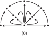
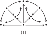
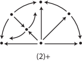
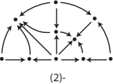
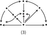
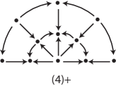
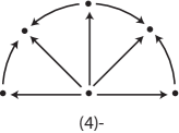
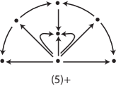
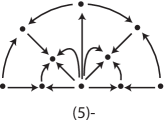
Figure 6. Phase portraits for normal form (I) in Proposition 5.3 for $\tilde{\lambda}>0$. Each diagram in [6][Figure 5.1] gives rise to two cases, depending on the choice of sign, numbering refers to their cases. In cases (0), (1) and (3) the two choices give equivalent phase portraits, case (0) is missing from [6]. Only half the disk is shown, the other half is obtained by rotation of $\pi$ around the origin. The equator of the Poincaré sphere is a global attractor in case (4)- and there is a polycycle in case (4)+.

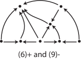
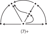
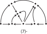
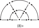
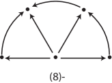
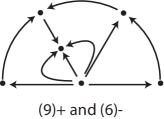
Figure 7. Phase portraits for normal form (V) in Proposition 5.3 for $\tilde{\lambda}>0$. Each diagram in [6][Figure 5.1] gives rise to two cases, depending on the choice of sign, numbering refers to their cases. Cases (6)$\pm$ and (9)$\mp$ coincide. The equator of the Poincaré sphere is a global attractor in case (8)- and there is a polycycle in case (8)+. Conventions as in Figure 6.

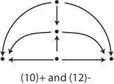
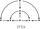
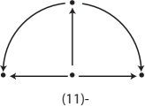
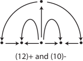
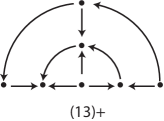
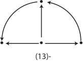
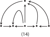
Figure 8. Phase portraits with $\tilde{\lambda}>0$ for normal forms (III), (VII) and (VIII) in Proposition 5.3, where there are 4 infinite equilibria. Numbering refers to cases in [6][Figure 5.1]. Cases (10)–(12) correspond to both (III) and (VIII) with (10)$\pm$ and (12)$\mp$ coinciding, (14)+ and (14)- are the same. Cases (13) and (14) arise for (VII). The equator of the Poincaré sphere is a global attractor in cases (11)- and (13)-. There is a polycycle in cases (11)+ and (13)+. Conventions as in Figure 6.

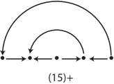
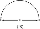
Figure 9. Phase portraits with $\tilde{\lambda}>0$ for normal forms (IV) and (IX), with two infinite equilibria, in Proposition 5.3. The equator of the Poincaré sphere is a global attractor in case (15)- and there is a heteroclinic cycle in case (15)+. Conventions as in Figure 6.

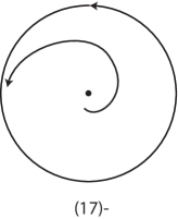
Figure 10. Phase portraits for normal forms (II) and (VI), with no infinite equilibria, in Proposition 5.3 for $\tilde{\lambda}>0$. The equator of the Poincaré sphere is a global attractor in case (17)- and there is a limit cycle in case (17)+. Conventions as in Figure 6.

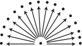
(a) and (d)

(b)

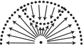
(c)

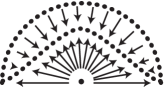
(e)

Figure 11. Phase portraits with $\tilde{\lambda}>0$ for normal form (X) in Proposition 5.3, when all points at infinity are equilibria. Cases (a)–(e) as in Lemma 5.4. Conventions as in Figure 6.

Acknowledgements:

The authors are grateful to R. Prohens and A. Teruel for fruitful conversations. The first author was partially supported by the Spanish Research Project MINECO-18-MTM2017-87697-P. The last two authors were partially supported by Centro de Matemática da Universidade do Porto (CMUP), financed by national funds through FCT - Fundação para a Ciência e a Tecnologia, I.P., under the project UIDB/00144/2020.

Appendix A Calculations for the examples with degree 2

Recall that ${\mathcal{F}}(x,y)=xQ_{2}(x,y)-yQ_{1}(x,y)$ and $g(\theta)={\mathcal{F}}(\cos\theta,\sin\theta)$.
Also let ${\mathcal{G}}(x,y)=xQ_{1}(x,y)+yQ_{2}(x,y)$ and $f(\theta)={\mathcal{G}}(\cos\theta,\sin\theta)$. In order to apply Proposition 3.4 we need to determine the sign of $f(\theta_{0})$ when $g(\theta)=0$.

Form (i)

${\mathcal{F}}(x,y)=(x+y)q(x,y)$ where $q(x,y)=x^{2}-xy+y^{2}$ is positive definite. Hence equilibria at infinity appear at $y=-x$, i.e. $\theta_{1}=-\pi/4$, $\theta_{2}=3\pi/4$

${\mathcal{G}}(x,y)=y^{3}+2q_{2}xy^{2}-2q_{1}x^{2}y-x^{3}$ hence ${\mathcal{G}}(x,-x)=2(q_{2}-q_{1}-1)x^{3}$.

Cases:
$q_{2}-q_{1}>1$  $\Rightarrow$ $f(\theta_{1})>0$ and $f(\theta_{2})<0$;
$q_{2}-q_{1}<1$  $\Rightarrow$ $f(\theta_{1})<0$ and $f(\theta_{2})>0$;
$q_{2}-q_{1}=1$  $\Rightarrow$ $f(\theta_{1})=f(\theta_{2})=0$.

Form (ii)

${\mathcal{F}}(x,y)=x(x^{2}-y^{3})$, equilibria at infinity at $x=0$ and $x=\pm\sqrt{3}y$ i.e. $\theta_{k}=(2k+1)\pi/6$, $k=0,\ldots,5$.

${\mathcal{G}}(x,y)=x(-x^{2}-2q_{1}xy+(2q_{2}-3)y^{2})$, hence
${\mathcal{G}}(0,y)=0$  and for $\varepsilon=\pm 1$ then ${\mathcal{G}}(\sqrt{3}y,\varepsilon y)=2\sqrt{3}y^{3}(q_{2}+\varepsilon\sqrt{3}q_{1}-3)$

Cases:
$q_{2}<3-\sqrt{3}q_{1}$ and $q_{2}\leq 3+\sqrt{3}q_{1}$  $\Rightarrow$ $f(\theta_{1})<0$ and $f(\theta_{3})\geq 0$;
$q_{2}\geq 3-\sqrt{3}q_{1}$ and $q_{2}>3+\sqrt{3}q_{1}$  $\Rightarrow$ $f(\theta_{1})\geq 0$ and $f(\theta_{3})<0$;
$q_{2}\geq 3-\sqrt{3}q_{1}$ and $q_{2}\leq 3+\sqrt{3}q_{1}$  $\Rightarrow$ $f(\theta_{1})\geq 0$ and $f(\theta_{3})\geq 0$;
$q_{2}<3-\sqrt{3}q_{1}$ and $q_{2}>3+\sqrt{3}q_{1}$  $\Rightarrow$ $f(\theta_{1})<0$ and $f(\theta_{3})<0$.

Form (iii)

${\mathcal{F}}(x,y)=3x^{2}y$, equilibria at infinity at $x=0$ and $y=0$ i.e. $\theta_{k}=k\pi/2$, $k=0,\ldots,3$.

${\mathcal{G}}(x,y)=xy(2q_{2}y+(2q_{1}-3)x)$, hence ${\mathcal{G}}(x,0)={\mathcal{G}}(0,y)=0$ i.e. $g(\theta)=0$  $\Rightarrow$ $f(\theta)=0$.

All equilibria at infinity are saddle-nodes.

Form (iv)

${\mathcal{F}}(x,y)=x^{3}$, equilibria at infinity at $x=0$ i.e. $\theta_{k}=k\pi$, $k=0,\ldots,1$.

${\mathcal{G}}(x,y)=x(2q_{2}y^{2}+2q_{1}xy-x^{2})$, hence ${\mathcal{G}}(x,0)=0$ i.e. $g(\theta)=0$  $\Rightarrow$ $f(\theta)=0$.

The equilibrium at infinity at $\theta_{0}$ is a non-hyperbolic attractor, at $\theta_{1}$ a non-hyperbolic repellor.

Form (v)

${\mathcal{F}}(x,y)=0$, all points at infinity are equilibria .     ${\mathcal{G}}(x,y)=2xy(q_{1}x+q_{2}y)$.

Cases:
$q_{1}=0$, $q_{2}\neq 0$  $\Rightarrow$ $f(\theta)\geq 0$  $\Leftrightarrow$ $q_{2}x\geq 0$;
$q_{1}\neq 0$, $q_{2}=0$  $\Rightarrow$ $f(\theta)\geq 0$  $\Leftrightarrow$ $q_{1}y\geq 0$;
$q_{1}q_{2}>0$  $\Rightarrow$ $f(\theta)\geq 0$  $\Leftrightarrow$ either ($x\geq 0$ and $y\geq 0$) or ($xy\leq 0$ and $q_{2}y\leq-q_{1}x$);
$q_{1}q_{2}<0$  $\Rightarrow$ $f(\theta)\geq 0$  $\Leftrightarrow$ either ($x\leq 0$ and $y\geq 0$) or ($xy\geq 0$ and $q_{2}y\leq-q_{1}x$).

References

- [1] M.J. Álvarez, A. Gasull and R. Prohens, Limit cycles for cubic systems with a symmetry of order 4 and without infinite critical points, Proceedings of the AMS, 136(3), 1035–1043 (2008).
- [2] A. Bendjeddou, J. Llibre and T. Salhi, Dynamics of the polynomial differential systems with homogeneous nonlinearities and a star node, J. Differential Equations 254, 3530–3537, (2013).
- [3] R. Benterki and J. Llibre, Limit cycles of polynomial differential equations with quintic homogeneous nonlinearities, Journal of Mathematical Analysis and Applications, 407, 16–22, (2013).
- [4] R. Boukoucha. Explicit limit cycles of a family of polynomial differential systems, Electronic J. Differential Equations, 217, 1–7, (2017).
- [5] M. Carbonell and J. Llibre. Limit Cycles of Polynomial Systems with Homogeneous Non-linearities, J. Math. Analysis and App., 142, 573–590, (1989).
- [6] A. Cima and J. Llibre. Algebraic and Topological Classification of the Homogeneous Cubic Vector Fields in the Plane. J. Math. Analysis and App., 147, 420–448, (1990).
- [7] A. Cima, A. Gasull and V. Mañosa. Phase portraits of random planar homogeneous vector fields, Qualitative Theory of Dynamical Systems, 20, 1–27 (2021).
- [8] B. Coll, A. Gasull and R. Prohens. Differential equations defined by the sum of two quasi-homogeneous vector fields, Can. J. Math., 49(2), 212-231, (1997).
- [9] C.B. Collins. Algebraic classification of homogeneous polynomial vector fields in the plane, Japan J. Indust. Appl. Math., 13 63–91, (1996).
- [10] T. Date. Classification and analysis of two-dimensional real homogeneous quadratic differential equation systems, J. Differential Equations, 32, 311–334, (1979).
- [11] F. Dumortier, J. Llibre and J.C. Artes, Qualitative Theory of Planar Differential Systems, Springer-Verlag (2006).
- [12] J.D. García-Saldaña, A. Gasull and H. Giacomini. Bifurcation diagram and stability for a one-parameter family of planar vector fields, Journal of Mathematical Analysis and Applications, 413, 321-342, (2014).
- [13] A. Gasull, J. Yu and X. Zhang, Vector fields with homogeneous nonlinearities and amny limit cycles, Journal of Differential Equations, 258, 3286–3303, (2015).
- [14] J. Huang, H. Liang and J. Llibre, Non-existence and uniqueness of limit cycles for planar polynomial differential systems with homogeneous nonlinearities, Journal of Differential Equations, 265, 3888–3913, (2018).
- [15] I.S. Labouriau and A.C. Murza. Limit cycles for a class of -equivariant systems without infinite equilibria, Electronic Journal of Differential Equations 2016, number 122, 1–12, (2016)
- [16] J. Llibre, J. Yu and X. Zhang, On the limit cycles of the Polynomial Differential Systems with a Linear Node and Homogeneous Nonlinearities, International Journal of Bifurcation and Chaos, 24(5), 1450065–1–7, (2014).