Modeling satellite-based open water fraction via flexible Beta regression: An application to wetlands in the north-western Pacific coast of Mexico

Abstract

Carbon sequestration and water filtering are two examples of the several ecosystem services provided by wetlands. Open water mapping is an effective means to measure any wetland extension as these are comprised of many open water bodies. An economical, though indirect, approach towards mapping open water bodies is through applying geo-computational methods to satellite images. In this work we propose the flexible Beta regression (FBR) model to predict open water fraction from measurements of a water index. We focus on observations derived from two MODIS images acquired during the dry season of 2008 in Marismas Nacionales, a wetland located in the north-western Pacific coast of Mexico. A Bayesian estimation procedure is presented to estimate the FBR model; in particular, we provide details of a nested Metropolis-Hastings and Gibbs sampling algorithm to carry out parameter estimation. Our results show that the FBR model produces valid predictors of water fraction unlike the standard model. Our work is complemented by software developed in the R language and available through a GitHub repository.

I Introduction and Data

Wetlands are ecosystems which serve as feeding and refuge areas for fish and crustaceans. Also, they function as biological water filters, act as natural systems to control floods, provide a natural environment for the sequestration and long-term storage of carbon dioxide from the atmosphere; they are the largest natural source of methane to the atmosphere [1, 2].

In light of the above, modeling the dynamic of these ecosystems has gained a lot of attention in recent years. An indirect and economical way to study the dynamic of extensive wetlands is through modeling biophysical variables derived from satellite images [3]. For instance, in order to determine the seasonal dependent extension of a wetland, time series of moisture or water indices can be generated and analyzed for the detection of open water. Typically, these indices are obtained by combining different spectral bands of satellite products such as the Moderate Resolution Imaging Spectroradiometer (MODIS) or the Landsat mission.

Since the spatial resolution of a Landsat image (30 m) is higher than that of many MODIS products (250, 500 or 1000 m), it is sensible to classify open water in a Landsat image and then calculate the corresponding water fraction in the MODIS image. For instance, if a MODIS pixel contains 25 Landsat pixels and 12 of the latter are classified as open water, then the fraction of water in the MODIS pixel is 12/25. The success of this seemingly straightforward procedure depends on acquiring Landsat images with good quality data (e.g., cloudless and free of shadow clouds and artifacts). It is common that during an entire dry season, only one Landsat image meets this quality requirements. This precludes the generation of time series of water fraction of MODIS images from previously classified Landsat products. Generating MODIS time series of water indices, however, is a simple task. In [4] the authors found that among 14 moisture and water indices, the MODIS-based Modified Normalized Difference Water Index $\mbox{B}_{6}$ (MNDWI6), see [5], has the best performance in appropriately defining open water bodies based on moderate spatial resolution products (such as Landsat).

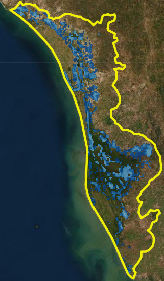
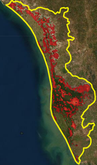
Figure 1: Marismas Nacionales (in yellow). (Left) Pixels of water fraction with good quality assessment (in blue). (Right) Pixels of MNDWI6 with good quality assessment (in red).

It is of interest to assess whether the MNDWI6 is an appropriate predictor of MODIS-based open water fraction which, in turn, was derived from a reference Landsat image. Should the MNDWI6 be a suitable predictor of open water then we shall use time series of this product for open water mapping thus circumventing the acquisition of spotless Landsat images.

In this work we provide an approach for modeling water fraction as a function of MNDWI6. Our application is tested on 2270 observations with good quality assessment. These observations were taken from two MODIS images with spatial resolution of 500 m, see Figure 1. These images were acquired on the 82 day of 2008, during the dry season of that year. The water fraction image was derived from a Landsat one (acquired on the same date) which was used to classify water presence; expert classification was applied to the Landsat image. These images include Marismas Nacionales whose 133,854 ha of estuaries, small patches of cedars, oaks, amapas and oil palm, coconut palm and white, red, black and Chinese mangrove, among other vegetation types, makes it the most important wetland in north-western Mexico; Marismas Nacionales is located at $22^{\circ}07\mbox{'}N$ and $105^{\circ}31\mbox{'}W$ [6].

A first modeling approach consists of fitting a linear regression between the water fraction and the MNDWI6. This model yields the line displayed in Figure 2-A; the intercept and slope estimates of this model are $\hat{\beta}_{0}^{\mbox{\tiny{lrm}}}=0.6041$ and $\hat{\beta}_{1}^{\mbox{\tiny{lrm}}}=1.1142$, respectively. A scatterplot of the fitted values of this model against the water fraction variable, see Figure 2-B, reveals that this approach is not appropriate for modeling purposes; some of the values predicted by the linear model lie outside the interval $(0,1)$.

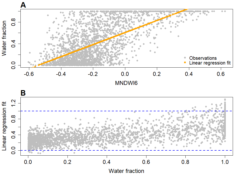
Figure 2: A Linear regression of MNDWI6 and water fraction. B Scatterplot of water fraction vs. fitted values.

In what follows we describe the novel flexible Beta regression (FBR) model which, by construction, takes into account that the response variable (water fraction) is bounded, hence, improving upon the linear model. Section II presents the basics of the FBR model, as well as details of the Bayesian estimation procedure employed to fit the FBR; a nested Metropolis-Hastings and Gibbs sampling algorithm is discussed. The routines needed for this algorithm were developed in the R language [7] and are available at the Github repository https://github.com/inder-tg/FBR. Results are presented in Section III and we provide an outlook of future work in the concluding Section IV.

II Methodology

Let $\boldsymbol{Y}^{\top}=(Y_{1},\ldots,Y_{n})$ denote $n$ independent response variables, each one taking values on the interval $(0,1)$. Flexible Beta regression was introduced by [8] as an alternative for modeling responses like $\boldsymbol{Y}$, which are bounded, as a function of some covariates. Briefly, we will discuss the main features of the flexible Beta regression model.

II-A On flexible Beta random variables

The density function of a flexible Beta random variable (rv) is given by

$$f_{FB}^{\ast}(y;\lambda_{1},\lambda_{2},\phi,p)=p\,f_{B}^{\ast}(y;\lambda_{1},\phi)+(1-p)\,f_{B}^{\ast}(y;\lambda_{2},\phi),$$ (1)

where $y\in(0,1)$, $0<\lambda_{2}<\lambda_{1}<1$, $\phi>0$, $p\in(0,1)$ and $f_{B}^{\ast}$ denotes the density of a mean-precision parametrized Beta rv:

$$f_{B}^{\ast}(x;a,b)=\frac{\Gamma(b)}{\Gamma(ab)\,\Gamma((1-a)b)}\,x^{ab-1}(1-x)^{(1-a)b-1},$$

where $x\in(0,1)$, $a\in(0,1)$, $b>0$.

That is, $f_{FB}^{\ast}$ is a mixture of two mean-precision Beta rvs with different means ($\lambda_{1}$ and $\lambda_{2}$) but with the same precision parameter ($\phi$). It is not difficult to see that the expected value of a rv with density function given by Eq.(1) is equal to $p\lambda_{1}+(1-p)\lambda_{2}$. The latter, gives rise to a reparametrization of the flexible Beta: $\mu=p\lambda_{1}+(1-p)\lambda_{2}$, $\phi=\phi$, $\tilde{\omega}=\lambda_{1}-\lambda_{2}$ and $p=p$. This reparametrization has proven useful in enhancing parameter interpretability in the flexible Beta regression model.

The flexible Beta density has a wide range of shapes, from unimodal, monotone and U-shaped to heavy-tailed. This characteristic makes it attractive to describe the main features of a broad group of variables with applications in several scientific fields. In addition to this, under mild conditions, it is known that two elements of the FB parametric family are equal if and only if the corresponding parameters are the same (see Proposition 1 of [8]), this type of strong identifiability property is typically found in non-mixture models.

II-B The flexible Beta regression model

Let us suppose that the $i$-th response variable, $Y_{i}\in(0,1)$, is linked to the vector of covariates $\boldsymbol{x}_{i}\in\mathbb{R}^{k}$. The flexible Beta regression (FBR) model consists of assuming that each $Y_{i}$ is independently distributed flexible Beta; in notation, $Y_{i}\sim FB(\mu_{i},\phi,\omega,p)$ where for some link function $g:[0,1]\to\mathbb{R}$,

$$g(\mu_{i})=\mathbb{E}[Y_{i}\mid\boldsymbol{x}_{i}]=\boldsymbol{x}_{i}^{\top}\,\boldsymbol{\beta},\quad\boldsymbol{\beta}\in\mathbb{R}^{k},$$ (2)

and $\tilde{\omega}=\omega\,\min\{\mu_{i}/p,(1-\mu_{i})/(1-p)\}$. Observe that this representation allows the parameters $\mu_{i}$, $\omega$ and $p$ to vary freely on $(0,1)$ and $\phi>0$. The parameter $\boldsymbol{\beta}$ is unknown.

Note also that the representation induced by the FBR model is equivalent to requiring that

$$\lambda_{1} =\mu_{i}+(1-p)\,\tilde{\omega}$$

$$\lambda_{2} =\mu_{i}-p\,\tilde{\omega},$$ (3)

in Eq.(1). So that, in what follows we will use the notation $f_{FB}^{\ast}(\cdot;\mu_{i},\phi,\omega,p)$ to refer to the density associated to an observation of the FBR model. For our application, we will consider the logit as the link function in Eq.(2). We remark that the flexible Beta regression is not a generalized linear model as the distribution of mixture of Betas does not belong to the exponential family.

II-C Bayesian estimation

Let $\boldsymbol{y}^{\top}=(y_{1},\ldots,y_{n})$ denote $n$ independent observations of the FBR model just introduced. The likelihood function of this model is by definition

$$\mathscr{L}(\boldsymbol{\eta}\mid\boldsymbol{y})=\prod_{i=1}^{n}\,f_{FB}^{\ast}(y_{i}\mid\mu_{i},\phi,\omega,p),$$ (4)

where $\boldsymbol{\eta}=(\boldsymbol{\beta},\phi,\omega,p)$. According to Proposition 2 of [8], this function is bounded from above almost surely, which ensures the existence of a finite global maximum on the parameter space. This result provides computational tractability to the FBR model, in particular for Bayesian estimation algorithms.

The underlying assumption of the FBR is that there are two groups of observations and the mean of one of these groups dominates the other, see Eq.(II-B). Given the $i$-th observation, however, we do not know to which of the two mixture components belongs. This makes the optimization of Eq.(4) unfeasible. To ameliorate this, a Bayesian approach is chosen, in particular, a data augmentation one is devised. More precisely, define the $n$-dimensional random vector $\boldsymbol{v}$ with entries

$$v_{i}=\begin{cases}1&\mbox{ if }y_{i}\mbox{ belongs to the first mixture component,}\\ 0&\mbox{ otherwise }\end{cases}.$$

Although essentially these latent variables ($\boldsymbol{v}$) are missing data, they can be included in the model and used for parameter estimation in a 2-step algorithm. In the first step, the parameter posterior distribution is obtained conditional on $\boldsymbol{v}$, and in the second step, the observations are classified ($\boldsymbol{v}$ is updated) conditional on knowing the parameter.

A key element in this algorithm is the complete-data likelihood function:

$$\mathscr{L}_{CD}(\boldsymbol{\eta}\mid\boldsymbol{y},\boldsymbol{v})=\prod_{i=1}^{n}\,\left[pf_{B}^{\ast}(y_{i};\lambda_{1},\phi)\right]^{v_{i}}\left[(1-p)f_{B}^{\ast}(y_{i};\lambda_{2},\phi)\right]^{(1-v_{i})},$$ (5)

where $\lambda_{1}$ and $\lambda_{2}$ are given by (II-B). Thus, given an appropriate prior distribution $\pi(\boldsymbol{\eta})$, the resulting posterior distribution is:

$$\pi(\boldsymbol{\eta},\boldsymbol{v}\mid\boldsymbol{y})\propto\mathscr{L}_{CD}(\boldsymbol{\eta}\mid\boldsymbol{y},\boldsymbol{v})\,\pi(\boldsymbol{\eta}).$$

Since there is no prior information available about the response variables utilized in our application, and, as we argued above, the parameters of the FBR model are strongly identifiable (also known as variation independent), it is sensible to assume a factorized joint prior distribution:

$$\pi(\boldsymbol{\eta})=\pi(\boldsymbol{\beta})\,\pi(\phi)\,\pi(\omega)\,\pi(p).$$ (6)

Following [8] and [9], in our application, we used a $k$-dimensional Gaussian prior $\boldsymbol{\beta}\sim\mathscr{N}_{k}(\boldsymbol{0},\Sigma_{\boldsymbol{\beta}})$ for the regression parameters; we employed a gamma prior distribution $\phi\sim\mathscr{G}(g,g)$ for the precision parameter, a rather usual choice, see e.g. [10]; and we chose non-informative uniform priors for the parameters $\omega\sim\mathscr{U}(0,1)$ and $p\sim\mathscr{U}(0,1)$. The $k\times k$ matrix $\Sigma_{\boldsymbol{\beta}}$ has large values in its main diagonal and zeroes otherwise. In the next section we provide details about the algorithm that allows us to fit the FBR model based on the complete-data approach just presented.

II-D Nested Metropolis-Hastings and Gibbs sampling

Some parameters of the FBR model have known conditional posterior distributions, whereas the posterior distribution of others have to be calculated numerically. For instance, it is not difficult to see that

$$\pi(v_{i}\mid y_{i},\boldsymbol{\eta})=\mbox{Bernoulli}(\pi(v_{i}=1\mid y_{i},\boldsymbol{\eta})),$$ (7)

where

$$\pi(v_{i}=1\mid y_{i},\boldsymbol{\eta})=\frac{p\,f_{B}^{\ast}(y_{i}\mid\lambda_{1},\phi)}{p\,f_{B}^{\ast}(y_{i}\mid\lambda_{1},\phi)+(1-p)\,f_{B}^{\ast}(y_{i}\mid\lambda_{2},\phi)}.$$

Note that by setting $n_{0}=\#\{t\mid v_{t}=0\}$ and $n_{1}=\#\{s\mid v_{s}=1\}$,

$$\pi(p\mid\boldsymbol{v})=\mbox{Beta}(n_{1}+1,n_{0}+1).$$ (8)

Also, we get

$$\pi(\tilde{\omega}\mid\boldsymbol{\beta},p) =\mathscr{U}(0,r(\boldsymbol{\beta},p)),$$

$$r(\boldsymbol{\beta},p) =\min\left\{\frac{\mu_{i}(\boldsymbol{\beta})}{p},\frac{1-\mu_{i}(\boldsymbol{\beta})}{1-p}\right\},$$

$$\mu_{i}(\boldsymbol{\beta}) =\frac{\mbox{exp}(\boldsymbol{x}_{i}^{\top}\,\boldsymbol{\beta})}{1+\mbox{exp}(\boldsymbol{x}_{i}^{\top}\,\boldsymbol{\beta})}:=\mbox{logit}^{-1}(\boldsymbol{x}_{i}^{\top}\,\boldsymbol{\beta}),$$

$$\mbox{logit}(x) =\log\left(x/(1-x)\right),\quad x\in(0,1).$$ (9)

Samples from the conditional posterior distribution of $(\phi,\boldsymbol{\beta})$ given $(\boldsymbol{y},\boldsymbol{v},p,\tilde{\omega})$ are obtained through Metropolis-Hastings (M-H) algorithms, see Ch. 10 of [11]. In particular, for the conditional posterior of $\phi$ we employed a random walk as the states transfer (jumping) distribution. For the conditional posterior of $\boldsymbol{\beta}$ the jumping distribution is a bivariate normal with mean equal to the value of the chain in the previous step and covariance matrix $\Sigma_{J}$, a diagonal matrix.

The following pseudocode summarizes the main steps needed to obtain samples from the conditional posterior distribution $\pi(\boldsymbol{\eta},\boldsymbol{v}\mid\boldsymbol{y})$.

0:  $\boldsymbol{x}$, $\boldsymbol{y}$, nSamples, $p_{0}$, $\omega_{0}$, $\phi_{0}$, $\boldsymbol{\beta}_{0}$, $\sigma_{\phi}$, $g$, $\Sigma_{J}$, $\Sigma_{\boldsymbol{\beta}}$

0:  $\boldsymbol{\mu}^{(0)}=(\mbox{logit}^{-1}(\boldsymbol{x}_{1}^{\top}\,\boldsymbol{\beta}_{0}),\ldots,\mbox{logit}^{-1}(\boldsymbol{x}_{n}^{\top}\,\boldsymbol{\beta}_{0}))$,$\boldsymbol{\omega}^{(0)}=\omega_{0}\cdot\min\{\boldsymbol{\mu}^{(0)}/p_{0},(1-\boldsymbol{\mu}^{(0)})/(1-p_{0})\}$

  for $j=1$ to nSamples do

     $v_{\mbox{\tiny{posterior}}}\leftarrow\pi(\boldsymbol{v}\mid\boldsymbol{y},\boldsymbol{\omega}^{(j-1)},p_{j-1},\boldsymbol{\mu}^{(j-1)},\phi_{j-1})$

     $p_{j}\leftarrow\pi(p\mid v_{\mbox{\tiny{posterior}}})$

     $\boldsymbol{\mu}^{(j)}\leftarrow(\mbox{logit}^{-1}(\boldsymbol{x}_{1}^{\top}\,\boldsymbol{\beta}_{j-1}),\ldots,\mbox{logit}^{-1}(\boldsymbol{x}_{n}^{\top}\,\boldsymbol{\beta}_{j-1}))$

     $\boldsymbol{\omega}^{(j)}\leftarrow\pi(\tilde{\omega}\mid\boldsymbol{\mu}^{(j)})$

     $\phi_{i}\leftarrow\pi_{\mbox{\tiny{M-H}}}(\phi\mid\boldsymbol{y},v_{\mbox{\tiny{posterior}}},\boldsymbol{\mu}^{(j)},\boldsymbol{\omega}^{(j)},p_{j},\phi_{j-1},\sigma_{\phi},g)$

     $\boldsymbol{\beta}_{j}\leftarrow\pi_{\mbox{\tiny{M-H}}}(\boldsymbol{\beta}\mid\boldsymbol{x},\boldsymbol{y},v_{\mbox{\tiny{posterior}}},p_{j},\omega_{i},\phi_{j},\boldsymbol{\mu}^{(j)},\boldsymbol{\beta}_{j-1},\Sigma_{J},\Sigma_{\boldsymbol{\beta}})$

  end for

Details about burning periods, thinning, chain size and values of initial parameters of this algorithm will be provided in the next section.

Having the sequence of vectors $\boldsymbol{\beta}_{j}$, $j=1,\ldots,\mbox{nSamples}$, which are appropriate samples of the posterior distribution of the regression parameter $\boldsymbol{\beta}$, we computed the median of each column to estimate the coefficients of the FBR model (2):

$$\hat{\beta}_{r} =\mbox{median}(\boldsymbol{\beta}_{j}[,r]),\quad r=1,\ldots,k.$$

Similarly, $\hat{p}=\mbox{median}(p_{1},\ldots,p_{\mbox{\tiny{nSamples}}})$, $\hat{\boldsymbol{\mu}}=(\mbox{logit}^{-1}(\boldsymbol{x}_{1}^{\top}\,\hat{\boldsymbol{\beta}}),\ldots,\mbox{logit}^{-1}(\boldsymbol{x}_{n}^{\top}\,\hat{\boldsymbol{\beta}}))$ and $\tilde{\omega}_{\mbox{\tiny{opt}}}=\min\{\hat{\boldsymbol{\mu}}/\hat{p},(1-\hat{\boldsymbol{\mu}})/(1-\hat{p})\}$. Consequently, substituing these estimators in (II-B) we obtained the regression functions $\hat{\lambda}_{1}$ and $\hat{\lambda}_{2}$.

III Results

For our application we considered $n=2270$ observations of the water fraction product as the response variable ($y_{i}$) and an equal number of values of the MNDWI6 index as their corresponding covariates ($z_{i}$); each $y_{i}$ and $z_{i}$ were recorded at the same geographical position (pixel). We included an intercept in our regression model, hence, $\boldsymbol{x}_{i}^{\top}=(1,z_{i})$, that is, in the notation above, $k=2$.

For sampling from the conditional posterior distributions, we ran initially 20 chains each having size $\mbox{nSamples}=8000$. We used $\boldsymbol{\beta}_{0}=(\hat{\beta}_{0}^{\mbox{\tiny{lrm}}},\hat{\beta}_{1}^{\mbox{\tiny{lrm}}})$. Our results were stable across different values of $p_{0}$ and $\omega_{0}$; we used small values for the diagonal of $\Sigma_{J}$ whereas large values for the diagonal of $\Sigma_{\boldsymbol{\beta}}$. We tried different starting values for the chain of the precision parameter $\phi$. We found stable chains when $\phi_{0}$ was in a vicinity of 3, $\sigma_{\phi}=0.125$ and instead of using a $\mbox{Gamma}(g,g)$ we employed a $\mbox{Gamma}(\kappa\,g,g)$ where $\kappa=30,35$ and $g=0.1,0.2,0.3$.

As a burning strategy we discarded the first 4000 samples of each chain. The remaining samples passed through the following thinning procedure to ensure no serial dependence between the posterior samples. The empirical autocorrelation function (ACF) applied to each chain revealed different dependence levels (significant lags); we found 15 as the largest dependence level. Our thinning strategy was to segment the sequence of samples in non overlapping intervals such that the last member of a given interval and the first element of the next one were separated at least 15 units. Then, at random we selected some samples from these strategically separated intervals; we took 500 non correlated samples on each chain. Thus, for each parameter of the FBR model we ended up producing 10000 posterior samples. Figure 3 depicts posterior samples of $p$ and $\phi$ along with their corresponding ACFs. Similarly, Figure 4 portraits the histogram of the posterior distribution of the flexible Beta regression parameters $\beta_{0}$ and $\beta_{1}$ accompanied by their ACFs.

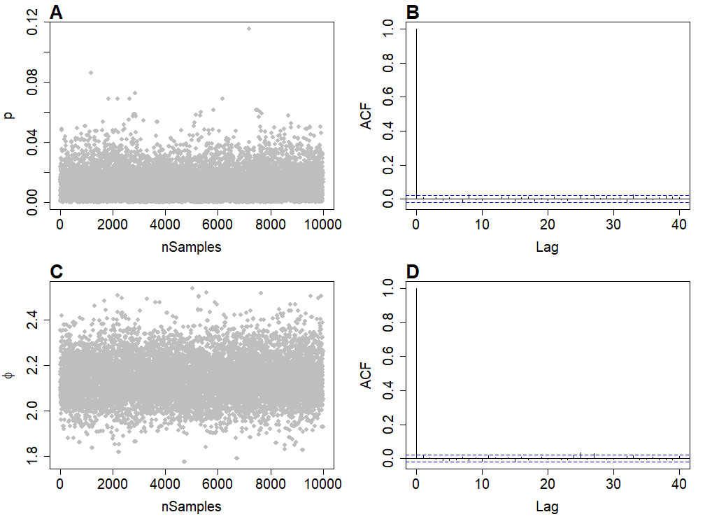
Figure 3: A-B Posterior samples of parameter $p$ with ACF. C-D Posterior samples of precision parameter $\phi$ with ACF.

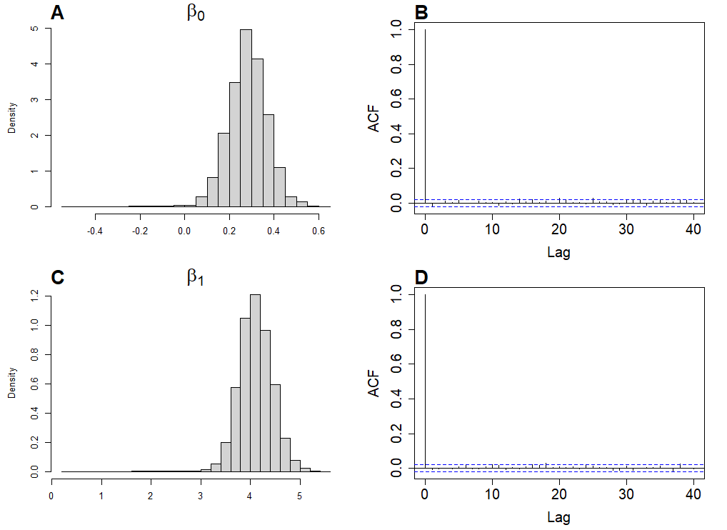
Figure 4: A-D Histograms and ACFs of the posterior distributions of the FBR parameters $\beta_{0}$ and $\beta_{1}$.

We consider that our implementation of the nested Metropolis-Hastings and Gibbs sampling algorithm and the subsequent application of our thinning approach produce appropriate posterior samples of the FBR model. In order to fit the FBR model we proceeded as explained at the end of Section II-D.

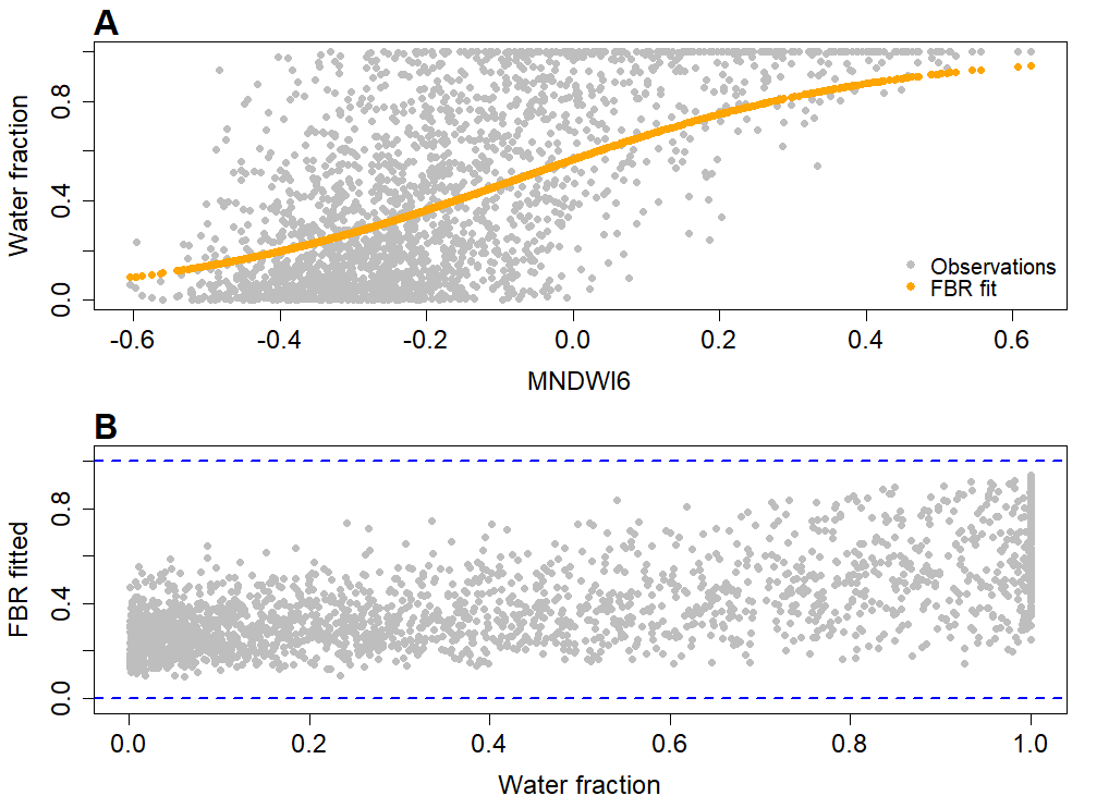
Figure 5: A Regression function $\hat{\lambda}_{2}$ (in orange) fitted via the FBR model. B Scatterplot of water fraction vs. FBR fitted values.

Figure 5-A shows the $\hat{\lambda}_{2}$ regression function fitted by the FBR model. As it is shown in Figure 5-B the predicted values of this model lie on the interval (0,1), satisfying the minimal requirement of a predictor of water fraction. The FBR model presented in this work is suitable for independent observations, which is a strong assumption to hold true on satellite-derived variables. In particular, the scatterplot of Figure 5-A shows levels of heteroscedasticity in the measurements. As argued by [8] the FBR can be used on heteroscedastic observations by allowing some parameters, for instance the precision parameter $\phi$, to depend on covariates. This modeling approach requires further study and it will be explored in the future.

IV Conclusions

Modeling water fraction measurements derived from satellite images can be construed as the first step in measuring the dynamic of open water bodies. In this work we presented the flexible Beta regression model as an alternative to predict water fraction as a function of the water index MNDWI6.

We have provided an algorithm based on Bayesian estimation principles to fit the FBR model. We consider that our implementation yields appropriate results and is available to any interested user. We have shown that the predicted values of the FBR model lie on the interval $(0,1)$. In this regard, this model improves the prediction made by the linear model.

Arguably, measurements of water fraction and water index are both spatially related. It is sensible to expect that this relation is still present when the measurements are vectorized (which is the type of data that we employed in this work). Our approach lacks of accounting for this apparent dependence between observations. It has been noticed by [8] that by allowing the precision parameter to depend on covariates it is plausible that the FBR model may be able to account for heteroscedasticity in the observations. We envision to explore this idea in our future research.

Subsequent steps for modeling open water fraction include the acquisition of biophysical and geographical variables such as precipitation, temperature, elevation and hydrological basin models and include them into our model. We believe that with this extra information along with the improvements discussed above our model will become a useful tool to assess the dynamics of the open water bodies of Mexico.

V Acknowledgment

We are grateful to Berenice Vázquez with CONABIO for kindly providing the images analyzed in this paper. Julia Trinidad Reyes was partly funded by Academia Mexicana de Ciencias through a summer grant during “Verano de la Investigación Científica 2020”.

References

- [1] W. Mitsch, B. Bernal, A. Nahlik, Ü. Mander, L. Zhang, C. Anderson, S. Jørgensen, and H. Brix, “Wetlands, carbon, and climate change,” Landscape Ecology, vol. 28, pp. 583–597, 2013.
- [2] S. Kirschke, P. and Bousquet, P. Ciais, M. Saunois, J. Canadell, E. Dlugokencky, P. Bergamaschi, D. Bergmann, D. Blake, L. Bruhwiler, and others, “Three decades of global methane sources and sinks, Nature Geoscience, vol. 6, pp. 813–823, 2013.
- [3] C. Prigent, E. Matthews, F. Aires, W. Rossow, “Remote sensing of global wetland dynamics with multiple satellite data sets,” Geophysical Research Letters, vol. 28, pp. 4631–4634, 2001.
- [4] R. Colditz, C. Troche-Souza, B. Vazquez, A. Wickel, and R. Ressl, “Analysis of optimal thresholds for identification of open water using MODIS-derived spectral indices for two coastal wetland systems in Mexico,” Int J of Appl Earth Obs Geoinf, vol. 70, pp. 13–24, 2018.
- [5] Hanqiu Xu, “Modification of Normalised Difference Water Index (NDWI) to enhance open water features in remotely sensed imagery,” International Journal of Remote Sensing, vol. 27, pp. 3025–3033, 2006.
- [6] National Commission for the Knowledge and Use of Biodiversity, “Mapa de uso del suelo y vegetación de la zona costera asociada a los manglares de México en 2015,” 1st. Ed. Mangrove Monitoring System of Mexico (SMMM), Mexico City, Mexico, 2016.
- [7] R Core Team, “R: A Language and Environment for Statistical Computing,” R Foundation for Statistical Computing, https://www.r-project.org/, 2016
- [8] S. Migliorati, A. Di Brisco, and A. Ongaro, “A new regression model for bounded responses,” Bayesian Analysis, vol. 13, pp. 845–872, 2018.
- [9] N. Bouguila, D. Ziou, and E. Monga, “Practical Bayesian estimation of a finite beta mixture through Gibbs sampling and its applications,” Statistics and Computing, vol. 16, pp. 215–225, 2006.
- [10] A. Branscum, W. Johnson, and M. Thurmond, “Bayesian beta regression: applications to household expenditure data and genetic distance between foot-and-mouth disease viruses,” Australian & New Zealand Journal of Statistics, vol. 49, pp. 287–301, 2007.
- [11] A. Gelman, J. Carlin, H. Stern, D. Dunson, A. Vehtari, and D. Rubin, Bayesian Data Analysis, CRC press, 2013.