An open-source automated magnetic optical density meter for analysis of suspensions of magnetic cells and particles

Abstract

We present a spectrophotometer (optical density meter) combined with electromagnets dedicated to the analysis of suspensions of magnetotactic bacteria. The instrument can also be applied to suspensions of other magnetic cells and magnetic particles. We have ensured that our system, called MagOD, can be easily reproduced by providing the source of the 3D prints for the housing, electronic designs, circuit board layouts, and microcontroller software. We compare the performance of our system to existing adapted commercial spectrophotometers. In addition, we demonstrate its use by analyzing the absorbance of magnetotactic bacteria as a function of their orientation with respect to the light path and their speed of reorientation after the field has been rotated by $90\text{\,}\mathrm{\SIUnitSymbolDegree}$. We continuously monitored the development of a culture of magnetotactic bacteria over a period of five days, and measured the development of their velocity distribution over a period of one hour. Even though this dedicated spectrophotometer is relatively simple to construct and cost-effective, a range of magnetic field-dependent parameters can be extracted from suspensions of magnetotactic bacteria. Therefore, this instrument will help the magnetotactic research community to understand and apply this intriguing micro-organism.

I Introduction

Magnetotactic bacteria biomineralize a chain of iron-oxide or iron-sulfide nanocrystals (a magnetosome) that makes them align with the Earth’s magnetic field [1, 2]. This property allows them to search efficiently for the optimal redox conditions in stratified water columns [3]. Ever since their discovery [4, 5] they have intrigued researchers in magnetism, not in the least because one can easily control them in a microscope [6, 7, 8]. Magnetotactic bacteria are used as model systems for many applications of magnetic particles, such as magnetic domain imaging [9, 10], hyperthermia [11, 12], magnetic particle imaging [13], microrobotic manipulation [14], targeted drug delivery [15, 16, 17, 18] and studies of spin-wave propagation [19].

Rosenblatt [20] discovered that the transmission of light through suspensions of magnetotactic bacteria is influenced by the direction of an externally applied field. This effect has been successfully applied as a simple method to monitor such processes as the cultivation of magnetotactic bacteria [21, 22, 23, 24] and to assess their velocity [25, 26].

I.1 Research question and relevance

Commonly, the field-dependent transmission of light through a suspension of magnetotactic bacteria is measured by extending a standard spectrophotometer with a magnetic add-on. Such spectrophotometers are also known as optical density meters, and are commonly used in biolabs to determine cell concentrations.

The modification of existing spectrophotometers with magnetic add-ons has several disadvantages. (i) These instruments are relatively complex and expensive, so modifications are usually made to depreciated equipment. (ii) Most instruments contain magnetic components that disturb the field and there is generally little space to mount electromagnets, certainly not in three dimensions. (iii) The various types of spectrophotometers and magnetic field generators and the variations between laboratories lead to a lack of a standardized measurement. (iv) More fundamentally, most spectrometers are not intended for sub-second continuous registration of absorbance over time. They are operated manually, and often use flash lamps.

In this publication, we present a spectrophotometer that intimately integrates the optical components with a magnetic field system and is dedicated to research on magnetotactic bacteria, see Figure 1. Additionally, the design considers that students at the Master’s or early PhD level should be capable of constructing such an instrument, both with respect to complexity and cost. Our main research question addresses how this new magnetic optical density meter, which we have dubbed MagOD, compares to existing adapted spectrophotometers, and what novel measurement strategies it enables.

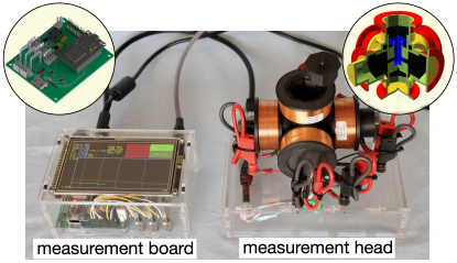
Figure 1: Photograph of an open-source spectrophotometer with magnetic field option (MagOD). The system consists of a measurement head (right) in which a cuvette with a suspension of magnetotactic bacteria is inserted. The measurement board (left) is dedicated to controlling the magnetic field, data acquisition and communication with the user over a touchscreen and WiFi. The design of the system is open, including the layout of the electronic circuit boards (top left), 3D print source files (top right) and control software.

I.2 Previous work

The system to be constructed is a spectrophotometer combined with a magnetic field system. It is therefore useful to compare it with commercial spectrophotometers. These systems generally use a xenon light source and monochromator with a wide wavelength range. Table 1 provides an overview of the specifications of representative commercial systems (Biochrome Ultrospecs and the Eppendorf Biophotometer used here for comparison), including their wavelength range $\lambda_{\text{min}}-\lambda_{\text{max}}$, spectral bandwidth $\Delta_{\lambda}$, maximum absorbance $O_{\text{D}}$ (see Eq. (3)) and approximate price.

The first spectrophotometer modified with a magnetic field module was presented by Schüler [27]. That device was based on standard optical components and used a permanent magnet to generate a $70\text{\,}\mathrm{m}\mathrm{T}$ field. Later versions were constructed around commercial optical density meters such as the ones presented by Lefèvre [25] (based on a Varian Cary 50 UV) and Song [24] (based on a Hitachi U2800). In their case, the magnetic field is generated by coil systems that can generate adjustable fields up to $6\text{\,}\mathrm{m}\mathrm{T}$ [25].

Table 1 also lists the parameters of the MagOD system introduced in this paper. Its optical properties and price range compare well with those of standard commercial systems, whereas its field range is similar to that of the adapted systems by Lefèvre and Song.

Table 1: Optical density meters.

	$\lambda_{\text{min}}$	$\lambda_{\text{max}}$	$\Delta_{\lambda}$	$O_{\text{D}}$	$B$	Price
	(nm)	(nm)	(nm)		(mT)	(Eu)
Ultrospec 8000	190	1100	0.5	8		12000
Biophotometer D30	230	600	4	3		5000
Ultrospec 10	600	600	40	2.3		1300
Schüler [27], 1995	637	637	18		70
Lefèvre [25], 2009	190	1100	1.5	3.3	0-6
Song [24], 2014	190	1100	1.5	6	0-4.3
MagOD	465	640	25	2	0-5	2000

I.3 Structure and contents

In this paper, we first discuss a model of the relationship between the transmission of light and the orientation of magnetotactic bacteria (Section II). Next to the specifications listed in Table 1, we defined other specifications that are important for analyzing magnetotactic bacteria and the open-source nature of the instrument. Our design choices are discussed in Section III. The results section is divided into two parts. In Section IV.1, we analyze the performance of our current implementation and compare it with a commercial optical density meter. Section IV.2 illustrates the possibilities of our novel system by giving four examples of experiments to extract information about the magnetic behavior of magnetotactic bacteria. This instrument is still very much a work in progress, and we invite the magnetotactic bacteria community to participate in its further development. For this purpose, we indicate possibilities for improvement and ideas for additional applications in Section V.

II Theory

The standard method to determine the proportion of bacteria with magnetosomes in a culture is to observe the changes of light transmitted through a suspension of bacteria under rotation of a magnetic field. This technique was pioneered by Rosenblatt [20]. The transmission of light is dependent on the relative orientation of the bacteria to the light path. For MSR-1, which are long, slender bacteria, transmission is high when the field is perpendicular to the light path, whereas it is low when the field is aligned parallel to the light path. This is somewhat counterintuitive, as MSR-1 have the smallest projected cross section when they are aligned along the line of view. (So in contrast to blinds, MSR-1 let light pass if the blinds are closed).

It is important to realize that we measure the intensity of light that reaches the photodetector. The light leaving the source can either be absorbed by the suspension of bacteria or scattered sideways so that it does not reach the photodetector. Highly dense suspensions of magnetotactic bacteria are milky white in appearance. Like milk, it is therefore very likely that magnetotactic bacteria scatter, rather than absorb, light. MSR-1 are small compared to the wavelength of the incident light, especially considering the size of their cross section. Additionally, their refraction index is only slightly higher than that of the surrounding liquid. These small “optically soft” objects scatter more light in forward direction if their projected area along the light path increases [28]. This would explain why the light intensity at the photodetector drops if the MSR-1 are aligned with the light beam.

For MSR-1, the projected area is roughly proportional to the sine of the angle between the long axis of the bacteria body and the light path. Owing to Brownian motion and flagellar movement, the bacteria will not be aligned perfectly along the field direction but show an angular distribution. The width of this distribution will decrease with increasing field. In the following discussion, we develop a simple theory to account for this effect. As the MagOD meter allows us to adjust the angle and strength of the magnetic field accurately, we can use it to validate the approximation.

II.1 Angle-dependent scattering $C_{\text{mag}}$

We define the angle between the light path and the MSR-1 long axis as $\alpha$, see Figure 2, and introduce a scattering factor relative to the intensity of light reaching the photodetector ($I(\alpha)$ with unit $\mathrm{V}$)

$$g(\theta)=\frac{I_{\text{max}}-I(\alpha)}{I_{\text{max}}-I_{\text{min}}}\,.$$ (1)

For MSR-1, the photodetector signal $I$ has a maximum when the MSR-1 are aligned perpendicular to the light beam ($I_{\text{max}}=I(90)=I_{\bot}$), at which point scattering $g(90)$ is minimal.

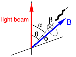
Figure 2: Definitions of various angles. In our MagOD system, we set the angle $\theta$ between the light path and the magnetic field $B$. The bacteria align with the direction of the field, but can deviate by a small angle $\phi$ in a cone around the field direction described by $\beta$. As a result, the angle between the bacteria long axis and the light is $\alpha$. In case of sufficiently large fields, $\phi=0$, $\alpha=\theta$, and $\beta$ is irrelevant.

Schüler [27] introduced a parameter to characterize the relative proportion of magnetotactic bacteria by comparing the light reaching the detector for the magnetic field aligned parallel and perpendicular to the light path ($C_{\text{mag}}$ denotes the “coefficient of magnetically induced differential light scattering” or the “ratio of scattering intensities” [29]). Assuming that the scattering intensity can be estimated from the reduction of light reaching the detector compared to the reference value of a sample without bacteria ($I_{\text{ref}}$), the original definition is

$$C^{*}_{\mathrm{mag}}=\frac{I_{\text{ref}}-I(0)}{I_{\text{ref}}-I(90)}\,.$$ (2)

With increasing concentration of bacteria, the total amount of light reaching the photodetector will decrease. In microbiology, cultures are traditionally characterized by “optical density”, a parameter that relates the reduction in light intensity to the reference value on a $10$-base log scale

$$O_{\text{D}}(\alpha)=\log\left(\frac{I_{\text{ref}}}{I(\alpha)}\right)=\log\left(I_{\text{ref}}\right)-\log\left(I(\alpha)\right)\,.$$ (3)

After the pioneering work of Schüler, researchers started to equip these optical density meters with magnetic fields [24, 29, 31, 32]. Using these instruments, it is more convenient to define $C_{\text{mag}}$ as

$$C_{\text{mag}}=\frac{O_{\text{D}\parallel}}{O_{\text{D}\bot}}=\frac{\log(I_{\text{ref}})-\log(I(0))}{\log(I_{\text{ref}})-\log(I(90))}\,.$$ (4)

Today, the latter definition is commonly used. However, it should be noted that the values are not identical, not even for $C_{\text{mag}}$ close to unity (see Appendix A). As $C_{\text{mag}}$ equals unity in the absence of magnetotactic bacteria, ($C_{\text{mag}}-1$) is often plotted [33, 29, 34, 23, 32].

In addition to the ratio, it is insightful to study the absolute difference between the absorbances in the parallel and perpendicular directions

$$\Delta_{\text{OD}} =O_{\text{D}\parallel}-O_{\text{D}\bot}$$

$$=\log(I(90))-\log(I(0))\,.$$ (5)

This difference is proportional to the absolute amount of magnetotactic bacteria that rotate in the field.

II.2 Dynamic response

When measuring $C_{\text{mag}}$ with adapted photospectrometers, the $O_{\text{D}}$ values are measured over a long interval, whereas the actual rotation of the bacteria is not measured. However, our MagOD system can measure at sub-second intervals and monitor the dynamic behavior of the bacteria. The response of bacteria to a change in field direction is determined by the balance between magnetic torque and rotational drag torque [35, 36, 37, 8]. Alignment of a bacterium to an external magnetic field with angle $\phi(t)$ (see Figure 2) can be described by a simple differential equation

$$f\frac{\partial\phi(t)}{\partial t}+mB\sin\phi(t)=0\,,$$ (6)

where $f$ [$\mathrm{N}\text{\,}\mathrm{m}\text{\,}\mathrm{s}$] represents the rotational drag coefficient, $m$ [$\mathrm{A}\text{\,}{\mathrm{m}}^{2}$] the magnetic dipole moment of the bacterium, and $B$ [$\mathrm{T}$] the magnetic field strength.

To determine $C_{\text{mag}}$, we rotate the field by $90\text{\,}\mathrm{\SIUnitSymbolDegree}$ very quickly. Therefore, we can initially assume the bacterium to be orthogonal to the magnetic field $\phi(0)=\nicefrac{{\pi}}{{2}}$. Solving the differential equation then yields

$$\phi(t) =2\cot^{-1}\exp{\left(\frac{mB}{f}t\right)}$$

$$\approx\frac{\pi}{2}\exp{\left(-0.85\frac{mB}{f}t\right)}\,.$$ (7)

This approximation is better than $0.065\text{\,}\mathrm{r}\mathrm{a}\mathrm{d}$ (see Appendix B). The angle $\phi$ can be estimated indirectly from the measured scattering as described by Eq. (1) if we assume that the bacteria remain in the plane of rotation ($\beta=0$). The settling time of this transition period is characterized by the time constant $\tau=f/mB$. As in our earlier work [8], we scale the response time to the magnetic field and introduce a general rotational velocity parameter $\gamma$ ($\mathrm{rad}\mathrm{/}\mathrm{T}\mathrm{s}$)

$$\gamma=\frac{m}{\pi f}=\frac{1}{\pi\tau B}\,.$$ (8)

From the response time an indication of the ratio between rotational drag coefficient and magnetic moment of single cells can be obtained [38, 8]. The rotational drag coefficient can be estimated from the bacteria shape using a spheroid approximation, slender body theory or measurement of macroscopic models in glycerol [36, 8].

II.3 Brownian motion

When we remove the magnetic field, magnetotactic bacteria will quickly reorient in a random orientation distribution via Brownian motion, and possibly via flagellar motion. For the same reason, the bacteria will not align perfectly along the magnetic field. The effect of Brownian motion on the alignment decreases with increasing fields, so we may expect $C_{\text{mag}}$ to be field-dependent. Let us first consider the effect of Brownian motion.

The probability distribution of finding magnetotactic bacteria tilted at an angle of $\phi_{0}$ from the magnetic field direction $b(\phi_{0})$ is determined by the ratio of magnetic ($-mB\cos(\phi)$) and thermal energy ($kT$) according to the Boltzmann distribution [20]. We should take into account that energy states for a specific value of $\phi$ exist in a full revolution around the field axis ($\beta=0\dots 2\pi$). Therefore

$$b(\phi_{0})= \frac{\int_{0}^{2\pi}e^{a\cos\phi_{0}}\sin(\phi_{0})d\beta}{\int_{0}^{\pi}\int_{0}^{2\pi}e^{a\cos\phi}d\beta d\phi}$$

$$= \frac{a}{2\sinh(a)}\sin(\phi_{0})e^{a\cos(\phi_{0})}\,,$$

where $a=mB/kT$, with $k$ ($\mathrm{J}\text{\,}{\mathrm{K}}^{-1}$) being the Boltzmann constant and $T$ ($\mathrm{K}$) the temperature.

To achieve a first-order approximation, we assume that the scattering factor is proportional to the projection of the bacteria shape onto the light direction. Defining $\alpha$ as the angle between the bacteria long axis and the light path, the scattering factor in Eq. (1) becomes

$$g(\alpha)=1-\lvert\sin(\alpha)\rvert\,.$$

The angle $\alpha$ is the combined result of the angle between the light and the field direction $\theta$ and the angle between the bacteria and the field $\phi$. One can show that the relation between $\alpha$ and these three angles is

$$\cos(\alpha)=-\sin(\theta)\sin(\phi)\cos(\beta)+\cos(\theta)\cos(\phi)\,,$$

resulting in the following expression for the scattering factor:

$$g(\theta,\phi,\beta)=1-\sqrt{1-\cos(\alpha)^{2}}\,.$$

The average scattering factor can be obtained by double numerical integration, first over all values of $\beta$ and then over the distribution of $\phi$

$$<g(\theta)>=\int_{0}^{\pi}g(\theta,\phi)b(\phi)d\phi\,.$$

The numerical integration was performed in Python, the source code of which is available as Supplementary Material (angular.py). Figure 3 shows the resulting average scattering factor as a function of the applied field angle for varying energy product $mB$. At an energy $mB$ well above $40\text{\,}\mathrm{k}\mathrm{T}$, the angular dependence approaches a $1-\sin(\theta)$ relationship.

Assuming a dipole moment of $0.25\text{\,}\mathrm{fA}\text{\,}{\mathrm{m}}^{2}$ as reported in our earlier work [8], $mB$=$40\text{\,}\mathrm{k}\mathrm{T}$ corresponds to a field of about $0.7\text{\,}\mathrm{m}\mathrm{T}$. Therefore fields on the order of a few mT may be sufficient to obtain the maximum value of $C_{\text{mag}}$.

When the field is removed, the scattering factor is $g_{0}=$0.2146$$. In this case, the intensity at the detector is $I_{0}=g_{0}I(0)+(1-g_{0})I(90)$, which we can relate to the average $O_{\text{D}}$ of the suspension

$$O_{\text{D}}= \log(\frac{I_{\text{ref}}}{I_{0}})$$

$$= -\log\left(g_{0}10^{-O_{\text{D}\parallel}}+(1-g_{0})10^{-O_{\text{D}\bot}}\right)\,.$$

In the above, we ignored the disturbing force caused by the flagella. Flagellar motion is complex [39], making the disturbing force difficult to calculate. However, we know that, in natural conditions, magnetotactic bacteria can use the Earth’s magnetic field of about $50\text{\,}\mathrm{\SIUnitSymbolMicro}\mathrm{T}$ to navigate. In this low field, $mB$ is only $3\text{\,}\mathrm{k}\mathrm{T}$. If the stochastic energy provided by the flagella is much greater than this value, the bacteria would not be able to follow the field. This suggests that, for fields on the order of mT, flagellar motion can be ignored.

Figure 3: Calculation of the average scattering factor as a function of the angle of the field with respect to the light incidence for varying values of the product of the magnetic moment of the magnetosome chain $m$ and the applied field $B$, expressed in units of $kT$ at room temperature. When all bacteria are perfectly aligned ($mB/kT=\infty$), the average scattering factor is inversely correlated to the projection cross section of the bacteria on the light path ($g=1-\sin(\theta)$). At lower fields, the loss of alignment reduces the angular dependence, which disappears for $mB<kT$.

III Method

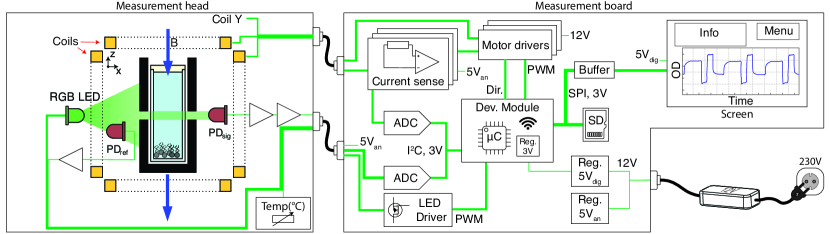
Figure 4: Diagram of the system: Measurement head: LED, refdiode, diode, amplifier stages, coils, cuvette, bacteria. Measurement board: outlet to 12 supply, $12\text{\,}\mathrm{V}$ to $5\text{\,}\mathrm{V}$ analog and digital, microcontroller, AD converter, LED driver, motor shields, current sense, HDMI cable, coil cable, SD card, WiFi. User interface: resistive touchscreen. Measurement board and user interface reside in the same housing.

Our MagOD system is an alternative to the modified commercial optical density meters currently used in magnetotactic bacteria research. It should therefore use compatible cuvettes and have comparable specifications. The preferred wavelength at which absorbance is measured is approximately $600\text{\,}\mathrm{n}\mathrm{m}$, and the maximum absorbance is approximately $1.4\text{\,}$ [25]. Intensity variations due to the change in direction of the magnetic field can be as high as $200\text{\,}\mathrm{\char 37\relax}$, but values as low as $2\text{\,}\mathrm{\char 37\relax}$ have been reported [24]. Although fields up to $70\text{\,}\mathrm{m}\mathrm{T}$ are applied [27], there are indications that saturation occurs as low as $2\text{\,}\mathrm{m}\mathrm{T}$ [24]. Our design therefore should have a wavelength of approximately $600\text{\,}\mathrm{n}\mathrm{m}$, an absorbance range of at least $1.5\text{\,}$, intensity resolution better than $1\text{\,}\mathrm{\char 37\relax}$, and a magnetic field above $2\text{\,}\mathrm{m}\mathrm{T}$.

The MagOD system has two main components, see Figure 4. The cuvette filled with the sample to be investigated is inserted into the measurement head, which holds the light source and photodetector circuit boards, the three coil sets and additional sensors (such as temperature). The measurement head is connected to the measurement board, which holds the analog-to-digital (AD) converters, the drivers for the magnetic field generation, and the light source. A microcontroller is mounted on the measurement board, which is connected over the board to the AD converters, the data storage card, and a touchscreen.

The design files for the hardware and software components are available at github.com/LeonAbelmann/MagOD.

III.1 Measurement head

We designed the measurement head to be as compact as possible to keep the volume and power consumption low. The dimensions of the standardized cuvette $12.5$$\times$$12.5$$\times$$45\text{\,}\mathrm{m}\mathrm{m}$) determine the size of the coil system, which essentially sets the outer dimensions of the measurement head. The circuit boards for the light source and sensors are embedded inside the coil system, with sensors located as close to the cuvette as possible.

III.1.1 Mechanical

As the measurement head carries all components, it is a complex structure that must be modified regularly to accommodate changes in component dimensions and added functionality. Therefore we decided to fabricate the structure by 3D printing so that modifications can be easily implemented. Printing in metal is still prohibitively expensive, so the measurement head itself cannot act as electromagnetic shielding. Instead, shields will have to be implemented on the circuit boards. However, it is possible to 3D-print with black nylon to shield the photodetector from external light and to allow the parts to be easily disinfected with a $70\text{\,}\mathrm{\char 37\relax}$ ethanol/water solution.

The measurement head consists of more than a dozen parts. The design is parameterized using the open-source OpenSCAD language, so that dimensions can be easily changed. The source files are available at github.

III.1.2 Coil system

We can choose between permanent magnets or electromagnets with or without cores to apply a magnetic field. As the field to be applied is relatively low, and the field direction needs to be changed rapidly to monitor the response of the bacteria, electromagnets without cores provide a simple, light weight solution. An additional advantage is that the field is directly proportional to the current, and there is no hysteresis, so no additional magnetic field sensors are required. The disadvantage of not having a core is that the maximum field is limited to a few mT. Higher fields can only be applied for short periods of time, limited by coil heating.

The magnetic field is generated by three orthogonal sets of two coils located on either side of the sample. The dimensions of the coils are more or less defined by the cuvette height, but we can choose the wire diameter to optimize the number of windings $N$. The field in the coil is proportional to the product of the current $I$ and $N$. The resistance $R$ of the coil scales approximately with $N^{2}$ for fixed coil dimensions. Therefore, the power dissipated in the coils ($I^{2}R$) is relatively independent of the number of windings for a given field strength. The inductance of the coil $L$ scales with $N^{2}$, so the cutoff frequency (proportional to $R/L$) is also fairly independent of the coil wire diameter. The choice of wire diameter is therefore determined mainly by the availability of power supplies, specifications of H-bridges and current ratings on connectors. Table 2 shows the specifications of two commercially available coils (Jantzen Audio 000-1235 and 000-0996) that are both suitable for our application. The number of turns was estimated from the coil resistance (using literature values for wire resistance) and the coil inductance [40]. Our MagOD system incorporates the coil with the higher number of windings ($996$) to benefit from the substantially lower currents, but at the expense of a slightly higher cutoff frequency and higher power consumption.

Table 2: Examples of coil specifications.

Jantzen Audio coil no.	1235	0996
Wire gauge	18	22	AWG
Wire diameter	1.0	0.64	mm
Resistance	21	53	$\text{\,}\mathrm{m}\mathrm{\SIUnitSymbolOhm}\mathrm{/}\mathrm{m}$
Inner diameter	42	42	mm
Outer diameter	57	53	mm
Height	21	21	mm
Inductance	0.94	2.9	mH
Resistance	0.5	2.1	$\text{\,}\mathrm{\SIUnitSymbolOhm}$
Cutoff frequency	85	115	Hz
Windings	$80(3)\text{\,}$	$140(7)\text{\,}$
Current for $1\text{\,}\mathrm{m}\mathrm{T}$	0.9	0.5	A
Voltage for $1\text{\,}\mathrm{m}\mathrm{T}$	0.44	1.1	V
Power	0.4	0.5	W

III.1.3 Temperature sensor

Electromagnets—especially those without cores—produce heat as a byproduct of the magnetic field. In the absence of active cooling, the temperature of the sample under investigation can rise quickly. This is especially problematic when one is working with micro-organisms. Therefore, it is important to monitor the temperature of the cuvette. The best option would be to insert a temperature sensor into the cuvette, but this method is cumbersome and risks exposing the sample to the outside air. The temperature of the coils can be estimated from their resistance, but that would overestimate the temperature of the cuvette. Therefore, we chose to mount a simple negative temperature coefficient (NTC) sensor in the housing as close as possible to the cuvette.

III.1.4 Light source

Ideally, the absorption pattern of a specimen is measured over a broad range of wavelengths. Most optical density meters use a wide-spectrum xenon flash lamp combined with a monochromator. However, this is not only a rather power-hungry, bulky solution ($>$$10\text{\,}\mathrm{W}$, $20\text{\,}\mathrm{m}\mathrm{m}$), it is also overkill for observing magnetotactic bacteria. Instead, we chose an RGB LED as source. LEDs are simple to control, can be mounted close to the cuvette, operated in continuous mode and easily adjusted in intensity using pulse width modulation (PWM). However, the wavelength cannot be chosen continuously, whereas the wavelength spectrum is determined by the LED type. Moreover, the wavelength bandwidth per color is rather large ($25\text{\,}\mathrm{n}\mathrm{m}$ compared to $5\text{\,}\mathrm{n}\mathrm{m}$ for monochromators). Finally, the light intensity of a LED is low compared to that of xenon lights or lasers. Based on the manufacturer’s data, the LED power in our current implementation is approximately $0.2\text{\,}$, $0.1\text{\,}$ and $0.7\text{\,}\mathrm{\SIUnitSymbolMicro}\mathrm{W}\mathrm{/}\mathrm{m}\mathrm{m}^{2}$ for $645\text{\,}$ (red), $520\text{\,}$ (green) and $460\text{\,}\mathrm{n}\mathrm{m}$ (blue) light, respectively. This is sufficient for most suspensions of magnetotactic bacteria.

The LED has a non-diffuse housing such that the light output in the direction of the sample is optimal. The LEDs can easily be exchanged, for instance for a yellow or UV LED, because they are mounted on a separate board.

The LED is mounted in common anode configuration such that (i) it can be driven by NPN MOSFETs and (ii) the supply difference between the LED ($5\text{\,}\mathrm{V}$) and the microcontroller ($3.3\text{\,}\mathrm{V}$) is inconsequential. The frequency of the PWM signal is well above the cutoff frequency of the photodetector amplifier. Since the brightness of LEDs decreases with time, we monitor the LED intensity. For this purpose a photodiode is placed in close vicinity before the light enters the cuvette.

III.1.5 Photodiode

The light passing the cuvette can be detected with photomultiplier tubes, avalanche photodiodes and silicon photodiodes [41]. Photomultipliers are highly sensitive, but are also quite bulky, require high voltages and perform less well at long wavelengths. Avalanche photodiodes are also very sensitive, but suffer from nonlinearity, noise, a high temperature dependence, and require high voltages to operate. As the transmission of light through most magnetotactic bacteria suspensions is high and we work at low acquisition frequencies, the sensitivity of silicon photodiodes is sufficient and allows us to take advantage of its small form factor, linearity and ease of operation. We used the more light-sensitive large-area photodiodes to boost sensitivity. The diode is operated in photovoltaic mode. In this mode, the bias voltage is zero, so the dark current, which is highly temperature-sensitive, is minimized.

In our MagOD implementation, the photodiode current is amplified by a two-stage operational amplifier (opamp) circuit because the signal is too weak for a single-stage amplifier. The first stage is a current-to-voltage converter. A low-noise JFET opamp is applied because this type of opamp has a low input current offset, which reduces DC errors and noise at the output. The first stage has the largest amplification in order to minimize the amplification of noise. The amplifier circuit is located directly behind the photodiode inside an electromagnetic protective casing, so that noise picked up by the cabling to the main board is not amplified and interference is minimized.

III.2 Measurement board

Placing the photodiode amplifier directly behind the photodiode is an effective way to suppress interference. We have the option to transport the amplified photodiode signal directly to the measurement board or to include the analog-to-digital (AD) converter next to the amplifier in the measurement head and convert the analog signal into a digital one. The analog option has the advantage of a small form factor for the circuit board and better access for testing. The digital option is more robust against interference and allows simpler cabling. As the current implementation of the MagOD system is very much a development instrument, we chose to move the AD converters to a separate measurement board, together with the microprocessor and other peripherals.

III.2.1 AD converter

The measurement board has two AD converters to read out the various analog signals on the system. As the measurements are normally performed on a longer time scale, we chose converters that are able to perform measurements with a sampling rate of up to $860\text{\,}\mathrm{Hz}$ and have integrated anti-aliasing filters. A 16-bit resolution provides an upper limit to the absorbance of 4.8, which is more than sufficient. In practice, the absorbance range is limited by stray light scattering around the sample.

The AD converters have a free-running mode, which performs measurements at an internally defined clock rate. A data-ready pin functions as an external interrupt such that the microcrontroller can be freed for other tasks while waiting for the AD converter to finalize its acquisition step.

III.2.2 Microcontroller

As data acquisition rates are low, the MagOD system can be easily controlled by a microcontroller ($\mu$C). This allows us to benefit from recent developments in low-cost, versatile $\mu$C development platforms. Rather than embedding the $\mu$C directly on the the electronic board, we chose to include it as a development board. This way, the system can be easily assembled, debugged and repaired.

The current implementation of the MagOD instrument is built around an ESP32 development board (Espressif Systems, Shanghai, China). The ESP32 $\mu$C has several characteristics that make it very suitable for this application: It has a small form factor, a fast 32-bit dual-core processor operating at $240\text{\,}\mathrm{MHz}$, WiFi and Bluetooth as well as several peripheral interfaces such as SPI and I²C. This $\mu$C is very popular, and numerous dedicated libraries, examples and discussions are available on Internet fora. Additionally, there is a plugin for the Arduino IDE, and many libraries are natively compatible, so even inexperienced developers can start with little effort.

III.2.3 Display

A resistive touchscreen enables the user to control the system with or without protective gloves. Additionally, the screen provides the user with information on the current and past states of the measurement and levels of the signals. Line drivers on the main board ensure that communication is reliable.

III.2.4 Storage

The acquired data and recipes are stored on a secure digital (SD) card. These cards are readily available in a variety of capacities, are widely applied in DIY projects, and are replaceable in case of a damaged card. The SD card can be interfaced to the $\mu$C in the SPI, the 1-bit SD, and the 4-bit SD modes. Although data transfer is faster in the 4-bit SD mode, we chose the SPI mode because it is well supported and the write speed is sufficient for our purpose. However, the write time to an SD card over an SPI interface using the ESP32 $\mu$C is unpredictable, with SD card-induced peaks in write time of at least $50\text{\,}\mathrm{m}\mathrm{s}$. Fortunately, the ESP32 has two cores, so unpredictable processes such as access to the SD card, reaction to touchscreen input and WiFi file transfers can be moved to a separate core.

III.2.5 Current drivers

The current through the coils must be controlled to obtain a specific magnitude of the magnetic field. We use PWM and benefit from the fact that the high inductance of the coil provides a low-frequency, low-pass filter for free. The use of PWM minimizes power dissipation in the supply, but results in a current ripple and consequently a ripple in the magnetic field. This ripple can be suppressed by choosing a sufficiently high PMW frequency. We use commercial motor drivers (Cytron MD13S) because they are specialized for driving high currents through a coil in two directions based on a simple two-wire control. The currently employed drivers work with frequencies up to $20\text{\,}\mathrm{kHz}$, suppressing the ripple by a factor of at least 100. The drivers can be interchanged by alternative motor drivers with similar capabilities.

The magnetic field is linearly dependent on the current. However, the current is not linearly dependent on the PWM duty cycle, as the internal resistance of the coil will vary due to temperature changes. A precise measurement of the current is necessary to close the loop and to assess the applied magnetic field. Therefore, a shunt resistor is placed in series with each coil. The voltage drop over this resistor is amplified using a current sensing amplifier and digitized with the AD converter. The measured signal can serve either to determine the true current or it can be applied in a feedback loop to compensate for coil heating.

III.2.6 Power supply

The measurement board electronics operate at low voltages ($3\text{\,}$ or $5\text{\,}\mathrm{V}$). However, the magnetic coil system is preferably operated at higher voltages to limit the currents and subsequent requirements for cabling and connectors. For reasonable winding wire diameters, the currents are in the range of a few ampere and the resistance of the coils is on the order of a few ohm. Therefore, we selected $12\text{\,}\mathrm{V}$ for the main on-board supply, for which a wide range of external power supplies is available and that even allows for operation from a car battery while in the field.

In our MagOD implementation, the three coil sets have a combined resistance of $4.2\text{\,}\mathrm{\SIUnitSymbolOhm}$ at room temperature. The maximum current is close to $3\text{\,}\mathrm{A}$ with $12\text{\,}\mathrm{V}$. This maximum current simultaneously through each coil set would require a maximum power supply of $120\text{\,}\mathrm{W}$.

The analog and digital circuits have a separate $5\text{\,}\mathrm{V}$ supply line to prevent noise originating from the switching nature of the digital circuitry from interfering with the measurement. The analog $5\text{\,}\mathrm{V}$ supply is built using an ultra-low-noise linear regulator, whereas the digital $5\text{\,}\mathrm{V}$ is built with a switching regulator. The latter is more efficient, but produces inherently more electronic noise. The $3\text{\,}\mathrm{V}$ needed for the $\mu$C originates from a linear regulator integrated on the development board.

III.2.7 Enclosure

The device is enclosed in a laser-cut plastic housing. Plastic was chosen because it does not block the WiFi signal. There is no need to deal with interference signals because the measurement signal is amplified in the measurement head, and the unshielded sections of the leads to the AD converter are kept very short.

The design is optimized such that no extra materials are needed for assembly. Additionally, the parts can be manufactured with a 3D printer. The source code for the enclosure design is available on github.

III.3 Cabling

While designing the MagOD system, we envisioned that measurements could take place inside controlled environments, such as incubators and refrigerators. Therefore the system was separated into two parts, connected by cabling. Components that did not have to be on the measurement head were moved to a separate module. This approach has the additional complication of requiring cabling and connectors. To mitigate this drawback, we chose commercially available cabling wherever possible.

For communication with the amplifier boards in the measurement head, we chose an HDMI cable, which features shielded twisted-pair wires with a separate non-isolated ground. HDMI cables are ideal for transmitting analog signals with low interference (5 V, signal, ground). The HDMI interface has evolved through several standards. The HDMI2.1 + Internet standard has five shielded twisted pairs that can be used for measurement signals (for instance three photodiodes, NTC and Hall sensor) and four separate wires that can be used for control signals (three LEDs). The connectors on the main board, amplifier boards and motor drives are standard Molex connectors. The coils are connected to standard measurement leads with banana connectors. The connection from the banana plugs to the measurement head is based on a Hirose RP 6-pole connector, which is the only cable that cannot be purchased in assembled form.

III.4 Software

Most modifications to the MagOD system will be made at the software level, which will be performed primarily by students. Generally speaking, (electrical) engineering students and many hobbyists are skilled in programming Arduino development boards. Therefore, the $\mu$C (ESP32) was programmed in the same way as an Arduino project, using C++ and the native Arduino IDE both as compiler and uploader. This has the major advantage of posing a negligible entry barrier for inexperienced $\mu$C programmers.

The disadvantage of the Arduino IDE is that it is not ideal for larger projects. The current implementation already exceeds 5000 lines of code. To partially relieve this issue, the code was set up in a highly modular way to assist new programmers in navigation, using only one main source file (.ino, .h) of 1000 lines, and several local library source files (src/*.cpp), e.g. for screen access, readout of the AD converter, writing to Flash memory, and WiFi access. The source code can be found on github.

The data is collected on the SD card and transferred over WiFi in a format that can be easily imported and displayed in a spreadsheet program. For more advanced analysis, Python scripts are available on github.

IV Results

We have analyzed the performance of our MagOD system, and shall compare it to a commercial spectrophotometer in the first part of this results section. To illustrate the possibilities of our novel instrument, we provide three examples in Section IV.2.

IV.1 Performance

Several iterations of MagOD systems have been realized based on the design considerations described in Section III. We expect that more iterations will follow, not only by our team but also by others in the field of magnetotactic bacteria. The most recent implementation can be found on github. We measured the performance of our MagOD meter (version 2) with respect to its optical and magnetic components to provide a baseline for future improvement.

IV.1.1 LED and photodetector

Photodetector sensitivity.

Our MagOD system is equipped with a three-color LED, which allows selection of three wavelengths (peak intensities at $645\text{\,}$, $520\text{\,}$ and $460\text{\,}\mathrm{n}\mathrm{m}$), either individually or in combination. The LEDs are individually driven by a PWM voltage to adjust their intensity, for instance to match the transmission of light through the liquid in the cuvette. A reference photodiode is mounted adjacent to the LEDs, which captures a small fraction of the LEDs’ light to monitor variations in the emitted light intensity. Figure 5 shows the signal of the detector and reference photodiodes as a function of the average LED power for the three wavelengths. The light pattern is shown in Figure 18 in the appendix, and a video is provided in the Supplementary Material (MagODLEDProjection.mov).

Space restrictions compelled us to design the two-stage amplifier such that the output decreases with increasing LED power. The reference photodiode, which has only one amplifier stage, has an increasing output with increasing intensity.

The relation between output voltage and intensity is linear for the red and green LEDs, but not for the blue LED at higher intensities. Measurements with liquids of different absorbance confirm that the sensitivity to blue light drops at high intensities of incident light, see Figure 19 in the appendix. Therefore, the blue LED should be used only for accurate absorbance at low incident power, i.e. for signals above $2\text{\,}\mathrm{V}$. At low intensity, the sensitivities of the red and blue channels are approximately equal, and twice as high as that of the green channel for the chosen combination of LED and photodetector. However, the sensitivity of the reference photodiode to red and blue light is clearly different. This again may be related to the placement of the diodes in the LED housing.

The linear fits to the data are listed in Table 3. The offsets are in agreement with the manufacturer’s specification of the ADS115 of $4.096\text{\,}\mathrm{V}$.

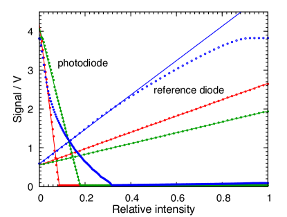
Figure 5: Photodiode and reference diode signal versus LED duty cycle (proportional to effective power). Note that the signal on the photodiode decreases with increasing light intensity due to the particular two-stage design of the amplifier. The reference diode amplifier is based on a conventional one-stage design. The photodiode signal is linear with the duty cycle for the red ($645\text{\,}\mathrm{n}\mathrm{m}$) and green ($520\text{\,}\mathrm{n}\mathrm{m}$) LEDs, but not for the blue ($460\text{\,}\mathrm{n}\mathrm{m}$) LED. Similarly, the reference diode signal is linear with the duty cycle of the red and green LEDs, but not for the blue. The parameters for the linear fits are listed in Table 3.

Table 3: Linear fits to measurements shown in Figure 5. The blue LED has a nonlinear response and is not tabulated.

		photodiode		reference diode
LED	$I_{\text{max}}$	offset	slope	offset	slope
	mA	V	V/$I_{\text{max}}$	V	V/$I_{\text{max}}$
Red	$20(2)\text{\,}$	$3.159(5)\text{\,}$	$-15.28(4)\text{\,}$	$0.545(3)\text{\,}$	$3.305(5)\text{\,}$
Green	$20(2)\text{\,}$	$3.168(2)\text{\,}$	$-6.696(9)\text{\,}$	$0.516(1)\text{\,}$	$1.902(2)\text{\,}$
Blue	$20(2)\text{\,}$			$0.532(1)\text{\,}$	$6.152(5)\text{\,}$

Absorbance validation.

To validate performance with respect to standard photospectroscopy measurements, we compared our MagOD system with a commercial optical density meter (Eppendorf BioPhotoMeter Plus). Figure 6 shows the absorbance ($O_{\text{D}}$) relative to water as a function of the wavelength of the light for a range of dilutions of a suspension of magnetic nanoparticles (FerroTec EMG 304). The transmission of light measured by our MagOD meter was averaged for a range of photodiode intensities ranging from zero to saturation. For the blue LED, however, care was taken to measure only at low intensities, where the response is linear, see Figure 5.

As expected, the absorbance increases with increasing nanoparticle concentration as indicated on the right-hand side of the graphs. The absorbance increases with decreasing wavelength, which is in agreement with the observation that the solution has a brown appearance. Care was taken to determine the accuracy of the measurement as accurately as possible. At this precision level, it is clear that our novel MagOD meter and the commercial instrument deviate, albeit never more than $0.2$ for absorbances below $2$. Above this value, the deviation becomes considerable, see data points inside dotted loop in Figure 6, probably due to light scattering onto the photodetector through other paths.

The blue LED seems to systematically underestimate the absorbance, which may be related to the fact that the response of the detector is ill-defined. The maximum absorbance is comparable to that of the commercial instrument. We therefore conclude that our MagOD instrument is satisfactory as a conventional absorbance meter, especially its red and green channels.

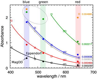
Figure 6: Absorbance relative to water measured with our MagOD meter (solid circles in the colored bands) for the three LEDs compared to the optical density measured by an Eppendorf BioPhotoMeter (open squares) measured as a function of wavelength. We used a range of dilutions of a water-based ferrofluid (FerroTec EMG 304), the dilution factor of which is indicated on the right. The data points for every dilution are indicated by a line to guide the eye. The difference between our MagOD meter and the commercial instrument is greater than the estimated measurement error, but less than $0.2$ for absorbances below $2$. Above this value, the estimate is unreliable (data points inside dotted loop). The absorbance of the blue LED is systematically lower than that of the commercial instrument. The maximum absorbance measured was $1.82$, which is slightly lower than for the commercial instrument ($2.14$). The measurement uncertainty is less than the symbol size and is therefore omitted for clarity.

Time response and noise level.

The ADS1115 AD converter has a maximum sampling rate of $860\text{\,}\mathrm{s}\mathrm{a}\mathrm{m}\mathrm{p}\mathrm{l}\mathrm{e}\mathrm{s}\mathrm{/}\mathrm{s}$, which means a sampling time of $1.2\text{\,}\mathrm{m}\mathrm{s}$. Figure 7 shows a time sequence of the sampled photodiode signal at that rate. The red LED was switched on and modulated from $46$ to $47$ bits on a full range of $255$ (relative intensity approximately $0.18$) every $250$ samples. The total acquisition of $1300$ samples took $4023\text{\,}\mathrm{m}\mathrm{s}$, so the effective sample rate was only $323\text{\,}\mathrm{s}\mathrm{a}\mathrm{m}\mathrm{p}\mathrm{l}\mathrm{e}\mathrm{s}\mathrm{/}\mathrm{s}$. The reduction in data rate is due to communication overhead with the AD converter, and could be optimized.

The data in Figure 7 shows two clear levels, with no measurement points in transition from one to the other. Therefore, we can safely conclude that the response of our MagOD meter at the highest sample rate is better than $3.1\text{\,}\mathrm{m}\mathrm{s}$. This is in agreement with the filter applied in the feedback loop of the amplifier, which has a $-3\text{\,}\mathrm{d}\mathrm{B}$ point at $800\text{\,}\mathrm{H}\mathrm{z}$ ($1.25\text{\,}\mathrm{m}\mathrm{s}$).

The ADS1115 has an internal filter that matches the bandwidth, which can be selected from discrete values of $8$, $32$, $64$, $128$, $250$, $475$ and $860\text{\,}\mathrm{s}\mathrm{a}\mathrm{m}\mathrm{p}\mathrm{l}\mathrm{e}\mathrm{s}\mathrm{/}\mathrm{s}$. Therefore, the noise should decrease at lower sample rates. Figure 8 shows the standard deviation of $1000$ samples, which is equal to the root-mean-square (RMS) noise as a function of sample rate. As expected, noise increases with increasing sample rate, but much more steeply than can be expected from a white noise spectrum, i.e. noise proportional to the square root of the bandwidth. There is a strong jump in noise above $64\text{\,}\mathrm{s}\mathrm{a}\mathrm{m}\mathrm{p}\mathrm{l}\mathrm{e}\mathrm{s}\mathrm{/}\mathrm{s}$, most likely caused by the presence of a $50\text{\,}\mathrm{H}\mathrm{z}$ cross-talk signal. At $64\text{\,}\mathrm{s}\mathrm{a}\mathrm{m}\mathrm{p}\mathrm{l}\mathrm{e}\mathrm{s}\mathrm{/}\mathrm{s}$ and below, the noise is on the order of $1\text{\,}\mathrm{b}\mathrm{i}\mathrm{t}$ or $125\text{\,}\mathrm{\SIUnitSymbolMicro}\mathrm{V}$. The full range of the detector circuit is $3.1\text{\,}\mathrm{V}$, which corresponds to a dynamic range of $88\text{\,}\mathrm{d}\mathrm{B}$ or a theoretical upper limit to the detectable absorbance of $4.4\text{\,}$. This compares very favorably to the commercial Eppendorf system, which has an optical-density resolution of $1\text{\times}{10}^{-3}\text{\,}$ on full range of approximately $2\text{\,}$. Assuming that the noise level of the Eppendorf system is comparable to the resolution, this would correspond to a dynamic range of only $53\text{\,}\mathrm{d}\mathrm{B}$.

At $64\text{\,}\mathrm{s}\mathrm{a}\mathrm{m}\mathrm{p}\mathrm{l}\mathrm{e}\mathrm{s}\mathrm{/}\mathrm{s}$, the noise level is $16\text{\,}\mathrm{\SIUnitSymbolMicro}\mathrm{V}\mathrm{/}\sqrt{Hz}$. SPICE simulations indicate that the theoretical noise level of the amplifier is on the order of $0.5\text{\,}\mathrm{\SIUnitSymbolMicro}\mathrm{V}\mathrm{/}\sqrt{Hz}$, indicating that we have not yet reached the full potential of the electronics.

Figure 7: Detector photodiode voltage sampled by the AD converter at a rate of $860\text{\,}\mathrm{s}\mathrm{a}\mathrm{m}\mathrm{p}\mathrm{l}\mathrm{e}\mathrm{s}\mathrm{/}\mathrm{s}$ while the red LED power is modulated by $0.4\text{\,}\mathrm{\char 37\relax}$. The effective sample rate was $323\text{\,}\mathrm{s}\mathrm{a}\mathrm{m}\mathrm{p}\mathrm{l}\mathrm{e}\mathrm{s}\mathrm{/}\mathrm{s}$. No transitions between the levels can be observed, so the time response of the detector photodiode is better than $3.1\text{\,}\mathrm{m}\mathrm{s}$.

Figure 8: Standard deviation (RMS noise) over $1000$ samples taken by the AD converter of the detector photodiode signal as a function of sample rate. Noise increases with increasing sample rate, but not proportional to the square root of the bandwidth (solid line). There is a strong increase in noise above $64$ samples/s.

IV.1.2 Magnetic field system

Figure 9 shows the magnetic field in the center of the system as a function of the current through each of the three coil sets. The coils generate approximately $2\text{\,}\mathrm{m}\mathrm{T}\mathrm{/}\mathrm{A}$, with around $5\text{\,}\mathrm{\char 37\relax}$ variation between the coils. The maximum field that can be generated is slightly higher than $5\text{\,}\mathrm{m}\mathrm{T}$ at full current of approximately $2.5\text{\,}\mathrm{A}$. The pulse width of the modulation of the driver circuits can be set with a maximum resolution of $16\text{\,}\mathrm{b}\mathrm{i}\mathrm{t}$, corresponding to a theoretical field resolution of about $70\text{\,}\mathrm{n}\mathrm{T}$. In practice, we operate the PWM at $8\text{\,}\mathrm{b}\mathrm{i}\mathrm{t}$ resolution, which yields a set-point resolution of about $20\text{\,}\mathrm{\SIUnitSymbolMicro}\mathrm{T}$.

As we drive the coils with a PWM signal, the current through the coils is not constant but follows the modulation frequency. At zero and maximum current, the ripple is absent. The ripple has a maximum at $50\text{\,}\mathrm{\char 37\relax}$ duty cycle. The filtering action of the coil system dampens the modulation. At a PWM drive frequency of $20\text{\,}\mathrm{k}\mathrm{H}\mathrm{z}$ and $50\text{\,}\mathrm{\char 37\relax}$ modulation, we measured a triangular current signal with a peak-to-peak amplitude of $24(2)\text{\,}\mathrm{m}\mathrm{A}$ on a mean current of $1.2\text{\,}\mathrm{A}$. Simulations considering only the low-resolution nature of the coils, with a corner frequency of $115\text{\,}\mathrm{H}\mathrm{z}$, yield a theoretical amplitude of $18\text{\,}\mathrm{m}\mathrm{A}$, so there is probably some additional capacitive coupling. The current variation corresponds to a maximum field variation in the field of approximately $50\text{\,}\mathrm{\SIUnitSymbolMicro}\mathrm{T}$ or $1.2\text{\,}\mathrm{\char 37\relax}$.

At the maximum current of $2.5\text{\,}\mathrm{A}$, the coils dissipate about $13.1\text{\,}\mathrm{W}$ each. As the coil system has no active cooling, the heating of the sample area can be considerable for prolonged measurement times. An NTC temperature sensor is mounted on the body of the measurement chamber to monitor the rise in temperature, see Figure 10. We also measured the temperature in the chamber with a simple alcohol thermometer for comparison. The temperature of the coils can be estimated from the increase in coil resistance, assuming the temperature coefficient of copper ($0.393\text{\,}\mathrm{\char 37\relax}\mathrm{/}\mathrm{K}$).

At a drive current of $0.5\text{\,}\mathrm{A}$ (field strength of $1\text{\,}\mathrm{m}\mathrm{T}$), the heating of the chamber is barely noticeable (about $1\text{\,}\mathrm{K}\mathrm{/}\mathrm{h}$). The average temperature of the coils increases at approximately $8\text{\,}\mathrm{K}\mathrm{/}\mathrm{h}$. With a drive current of $1.2\text{\,}\mathrm{A}$, the temperature of the coils increases by $21\text{\,}\mathrm{K}$. The temperature increase of the chamber is substantial, with an initial increase of approximately $0.25\text{\,}\mathrm{K}\mathrm{/}\mathrm{m}\mathrm{i}\mathrm{n}$ and a subsequent flattening at $7\text{\,}$ to $8\text{\,}\mathrm{K}$ after $40\text{\,}\mathrm{m}\mathrm{i}\mathrm{n}$.

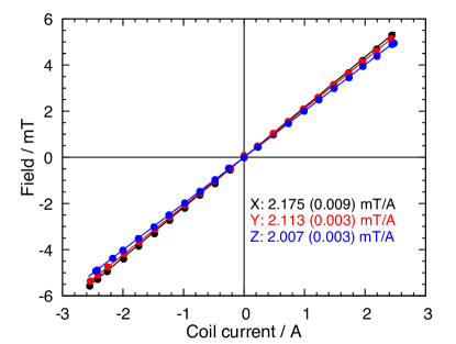
Figure 9: Magnetic field in the center of the cuvette holder as a function of average coil current. Fields in $x$, $y$ and $z$ direction with a field-to-current ratio of $2.175(9)\text{\,}$, $2.113(3)\text{\,}$ and $2.007(3)\text{\,}\mathrm{m}\mathrm{T}\mathrm{/}\mathrm{A}$, respectively.

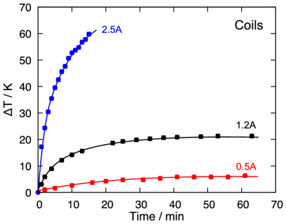
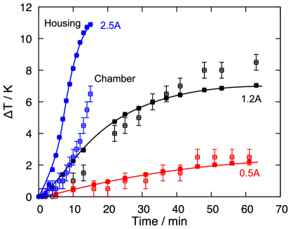
Figure 10: Top: Temperature of the coil system as a function of time for different drive currents. At the maximum drive current of $2.5\text{\,}\mathrm{A}$, corresponding to $5\text{\,}\mathrm{m}\mathrm{T}$, the coils heat rapidly, and operation should be limited to a few minutes. Bottom: MagOD frame temperature (solid symbols) and air temperature in the chamber (open symbols) as a function of time. At a drive current below $1.2\text{\,}\mathrm{A}$ ($2.4\text{\,}\mathrm{m}\mathrm{T}$), the temperature increase of the frame is limited to about $6\text{\,}\mathrm{K}$.

IV.2 Applications

We present four experiments to illustrate the application of our MagOD meter to analyze magnetotactic bacteria. We measure (1) the scattering of Magnetospirillum gryphiswaldense (MSR-1) bacteria as a function of their angle to the incident light, (2) their rotational velocity as a result of a rotation of the external magnetic field on time scales of seconds and (3) the development of a culture over a period of several days. The final experiment measures (4) the velocity distribution of the unipolar Magnetococcus marinus (MC-1) as a function of time.

IV.2.1 Transmission as a function of angle (MSR-1)

Using the coil system of our MagOD meter, we can apply a field in any direction in three-dimensional space. This allows us to study the transmission of light as a function of the orientation of the bacteria and check the model presented in Section II.

For this purpose, a cuvette of MSR-1 bacteria, grown as described in reference [8], with an optical density of approximately $0.1\text{\,}$ was inserted into the MagOD system. We measured the intensity on the photodetector as a function of the angle of the magnetic field with steps of approximately $5\text{\,}\mathrm{\SIUnitSymbolDegree}$. The magnetic field varied with angle, but was always greater than $1\text{\,}\mathrm{mT}$. As the optical density of the sample fluctuated continuously due to activity and sedimentation within the cuvette, we performed the measurement $20$ times. The resulting curves were normalized to a range of $0$ to $1$ and averaged to obtain the angle-dependent scattering factor $g(\theta)$ shown in Figure 11.

The simple inverted sine model discussed in Section II fits surprisingly well. The strongest deviation is around the parallel alignment, which is not surprising. The MSR-1 are not infinitely thin rods, but spirals. Therefore, the projected area will be less sensitive to variations in the angle around the long axis. Additionally, the culture of MSR will have a distribution in angles (due to Brownian motion and/or flagellar motion), which will round off the sharp corner at $\theta=0$. The red curve illustrates this effect for $mB$=$60\text{\,}\mathrm{k}\mathrm{T}$, which still does not fit the measurement very well. It therefore seems likely that the actual bacteria shape, and might also be their distribution, should be included in the model.

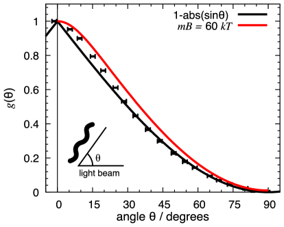
Figure 11: Scattering of a culture of magnetotactic bacteria is dependent on the orientation of the external magnetic field; it is highest when the field, and hence the bacteria, are aligned parallel to the light beam and lowest when the field is aligned orthogonally. By normalizing from $[0,1]$, we obtain the angle-dependent scattering factor $g(\theta)$, which can be relatively well approximated by a sine function. The flattening of the curve around $0\text{\,}\mathrm{\SIUnitSymbolDegree}$ can be partly explained by additional Brownian motion of the bacteria (red curve).

IV.2.2 Response as a function of field strength and time (MSR-1)

We most commonly perform measurements in which a sample of MSR-1 is subjected to field switching between parallel and perpendicular alignment to the light path and varying field strengths. Figure 12 shows the measured response for a set of field cycles. At a high field value of $3\text{\,}\mathrm{m}\mathrm{T}$, the field is switched from parallel to perpendicular alignment after $10\text{\,}\mathrm{s}$. For the lower field value of $0.4\text{\,}\mathrm{m}\mathrm{T}$, we can allow longer reversal times because coil heating is negligible.

From the difference in detector signals, we can calculate $\Delta_{\text{OD}}$ using Eq. (II.1). The signal of the growth medium without bacteria ($I_{\text{ref}}$) was $301(1)\text{\,}\mathrm{m}\mathrm{V}$. We can therefore calculate $C_{\text{mag}}$ using Eq. (4).

The difference in transmission between in-plane and perpendicular alignment is higher at $3\text{\,}\mathrm{m}\mathrm{T}$ compared to $0.4\text{\,}\mathrm{m}\mathrm{T}$. This is in agreement with the predicted increase of scattering factor with increasing field, see Figure 3. Figure 13 shows the calculated difference in scattering factor as a function of the magnetic field scaled to $kT/m$. From a previous analysis of MSR-1 [8], we estimated that the mean magnetic moment $m$ of the magnetosome chain is $0.25\text{\,}\mathrm{f}\mathrm{A}\mathrm{m}^{2}$, with a $10-$90\text{\,}\mathrm{\char 37\relax}$$ cutoff of the distribution of $0.07\text{\,}$ and $0.57\text{\,}\mathrm{f}\mathrm{A}\mathrm{m}^{2}$, respectively. We can convert these ranges of moments into the energy ratio $mB/kT$ for the two difference field values. Lines on the top axis of the graph indicate the ranges, and red circles on the red line indicate the mean values. The predicted reduction between the average scattering factors ($0.20\text{\,}$) at the two field values is less than that observed in Figure 12 ($0.5\text{\,}$). The discrepancy could originate from the fact that this simple model ignores disturbance caused by flagellar motion. Another plausible cause is a smaller average magnetic moment $m$ of the magnetosomes in this particular sample. Microscopy observations of trajectories of other wild-type MSR-1 show alignment for fields of $0.4\text{\,}\mathrm{m}\mathrm{T}$ [42], which is in agreement with the model.

In addition to a decrease in step height, the time response also decreases with decreasing field. The time constant is estimated from a fit of Eq. (7) to the data using the sum of squared errors criterion. The time constant of the transitions to $3\text{\,}\mathrm{m}\mathrm{T}$ is $1.7(5)\text{\,}\mathrm{s}$, which is approximately 13 times higher than the time constant of $5.4(8)\text{\,}\mathrm{s}$ of the transition to $0.4\text{\,}\mathrm{m}\mathrm{T}$. The ratio is rather high, but still within measurement error equal to the ratio of the fields, as predicted by the model discussed in Section II.

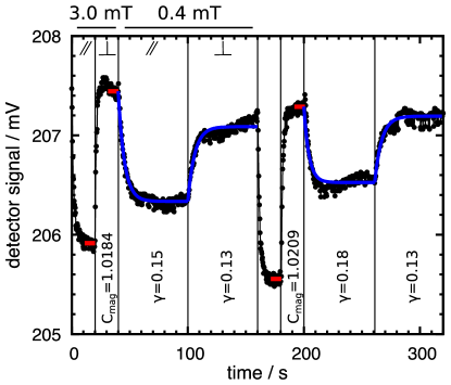
Figure 12: Two cycles of a measurement sequence. The magnetic field is alternatively aligned parallel and perpendicular to the light beam. For high fields ($3.0\text{\,}\mathrm{m}\mathrm{T}$), we can determine $\Delta_{\text{OD}}$ from the difference between the averages of the detector signals (red lines), from which we can calculate $C_{\text{mag}}$. The signal of the growth medium without bacteria was $301(1)\text{\,}\mathrm{m}\mathrm{V}$. The difference between the two directions of the field drops considerably at low field ($0.4\text{\,}\mathrm{m}\mathrm{T}$), whereas the response time increases. These low fields are suitable for estimating the time constant $\tau$ from a fit to an exponential (blue line). Using the field magnitude, we can calculate $\gamma$ ($\text{\,}\mathrm{r}\mathrm{a}\mathrm{d}\mathrm{/}\mathrm{m}\mathrm{T}\,\mathrm{s}$).

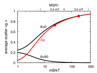
Figure 13: Calculation of the average scattering factor as a function of the product of the magnetic moment of the magnetosome chain $m$ and applied magnetic field $B$ for the magnetic field aligned parallel ($\theta$=$0\text{\,}\mathrm{\SIUnitSymbolDegree}$), and perpendicular ($\theta$=$90\text{\,}\mathrm{\SIUnitSymbolDegree}$) to the light path, see Figure 3. The difference in the average scattering factor between these orientations is indicated by a red line ($\Delta g$). From earlier work [8], we estimated that the mean magnetic moment of the magnetosome chain is $0.25\text{\,}\mathrm{f}\mathrm{A}\mathrm{m}^{2}$, with a $10-$90\text{\,}\mathrm{\char 37\relax}$$ cutoff of the distribution of $0.07\text{\,}$ and $0.57\text{\,}\mathrm{f}\mathrm{A}\mathrm{m}^{2}$, respectively. The resulting ranges in $mB/kT$ are indicated on the top axis and by red circles for the mean values of the moments for the fields used in the experiment illustrated in Figure 12.

IV.2.3 Comparison of $C_{\text{mag}}$ for different instruments

A major advantage of our novel MagOD system is that it allows us to standardize $C_{\text{mag}}$ measurements obtained at different laboratories. It is not trivial to calibrate instruments by sending around bacteria cultures because such cultures develop with time and are not stable. Therefore, a standard instrument is the better solution. Table 4 compares $C_{\text{mag}}$ with existing instruments in three different laboratories. Researchers at CNRS used a modified Cary UV at $600\text{\,}\mathrm{n}\mathrm{m}$ wavelength, those at Aston University used a modified Thermo Evolution at $565\text{\,}\mathrm{n}\mathrm{m}$ wavelength, and those at Bayreuth University used a Ultrospec 2100 Pro at $565\text{\,}\mathrm{n}\mathrm{m}$ wavelength as well. The cultures were not the same, so the results obtained at the above laboratories cannot be compared. Nevertheless, it is very clear that the difference between the results obtained from commercial instruments and those obtained from our standardized MagOD vary significantly from laboratory to laboratory.

Table 4: $C_{\text{mag}}$ of MSR-1. Comparison of MagOD with commercial instruments used at different laboratories (Cary UV: CNRS, Thermo Evolution: Aston, Ultrospec 2100: Bayreuth). The difference between commercial instruments and our MagOD system varies from laboratory to laboratory, which underscores the need for a standardized measurement instrument.

	Cary			Thermo	Ultrospec 2100
Commercial Inst.	2.8	3.1	2.8	2.4	2.6	2.4	2.2
MagOD Green	1.9	2.1	1.9	2.3	1.5	2.3	1.5
MagOD Red				2.5	1.7	1.6	1.7

IV.2.4 Long-term growth monitoring (MSR-1)

When cultivating magnetotactic bacteria such as MSR-1, it is important to check regularly whether the bacteria remain magnetic. When bacteria are grown under laboratory conditions, random mutation may lead to a culture of magnetotactic bacteria that has lost the ability to form magnetosomes [43]. In our lab, MSR-1 are grown in $2\text{\,}\mathrm{m}\mathrm{L}$ tubes. The tubes are closed, and a small headspace of air serves to ensure a proper reduction of oxygen concentration as the culture grows. Even though this method is simple, its major disadvantage is that we have no information whether the magnetosome formation occurs as we expect it to. We cannot open the tubes to take samples, because that would let oxygen in. The better option would be to grow the bacteria in bioreactors that allow sampling without disturbing the oxygen concentration. Unfortunately, bioreactors are complex, costly, and provide quantities that far exceed what is needed for lab-on-chip experiments.

Our MagOD system offers a solution for monitoring the growth of MSR-1 bacteria and the magnetosome by keeping cultures in cuvettes inside the MagOD meter for long periods. Throughout the growth period, we continuously measure the absorbance during changes of the external magnetic field. In this way, we obtain information about the total number of bacteria as well as their magnetic response.

We prepared MSR-1 cultures in the conventional manner [8] but, instead of tubes, we used quartz cuvettes with a PTFE stopper (Hellma QS 110-10-40) to avoid oxygen leakage into the cuvette. For the long-term observations shown in Figure 14, the magnetic field was set to loop through cycles of $100\text{\,}\mathrm{s}$ consisting of a vertical field of $1.0\text{\,}\mathrm{mT}$ ($20\text{\,}\mathrm{s}$), a horizontal field of $2.9\text{\,}\mathrm{mT}$ ($20\text{\,}\mathrm{s}$), and a vertical field of $0.1\text{\,}\mathrm{mT}$ ($60\text{\,}\mathrm{s}$).

The first transition is at a relatively strong field, thus guaranteeing reliable estimations of $C_{\mathrm{mag}}$. The second transition guarantees a relatively high time constant, which is helpful for estimating $\tau$ accurately.

Figure 14 shows the measured parameters of a sample of magnetotactic bacteria over a period of five days. The optical density, relative ($C_{\text{mag}}$) and absolute ($\Delta_{\text{OD}}$) magnetic response and relative rotation velocity ($\gamma$, proportional to the ratio between magnetic moment and rotational friction coefficient) are plotted from top to bottom. The optical density is typical for a bacteria growth sequence. After a lag phase L, a transition into the exponential growth phase E occurs, followed by the stationary phase S, where the bacteria concentration remains more or less constant. After three days, however, the density increases unexpectedly as illustrated in phase X. Since $\Delta_{\text{OD}}$ is decreasing, it seems unlikely this increase is caused by accelerated growth of bacteria or an increase in scattering due to an increase in intracellular storage granules.

During the exponential growth phase, $C_{\text{mag}}$ decreases within half a day. As $\Delta_{\text{OD}}$ remains constant, we hypothesize that the increase in cell density is entirely due to bacteria without magnetosomes. Only after two days do we see a gradual increase in magnetic signal due to an increase in the proportion of bacteria with magnetosomes. With the increase in magnetic signal, $\gamma$ also increases, hence the magnetic moment of the magnetosome increases compared to the average bacteria length. The observation for the first three days would be consistent with the mechanism that, after seeding with magnetic bacteria, growth first proceeds by an increase in non-magnetic bacteria. When that growth stops, the bacteria start to form magnetosomes. This mechanism contradicts electron microscope observations by Staniland and Yang that magnetosome crystals are distributed equally over both parts of the divided cell [44, 45]. Another hypothesis is that after cell division, the two daughter cells are shorter and therefore optically less anisotropic, leading to a reduction in $C_{\text{mag}}$. The division must be such that the the absolute change in absorbance by the two new cells, $\Delta_{\text{OD}}$, remains constant. This is far from obvious.

A sharp transition in phase X occurs after approximately $3.3$ days. As the density of the culture increases again, the magnetic response decreases but $\gamma$ continues to increase. This is a feature we often observe in these measurements( [46], appendix B). In this particular case the noise in $\gamma$ decreases, which was not observed in other experiments. Variations in culture growth over time between experiments are not uncommon, even under controlled conditions [22]. However, we sometimes observe a cloudiness in the suspension, which may be caused by aerotaxis or contamination. As we do not shake the suspensions before measuring like in a standard optical density meter, these clouds may float in front of the detector and complicate the analysis. It is possible that, rather than rotating individual bacteria, we rotate the entire cloud. Clearly, this type of experiment needs to be developed further.

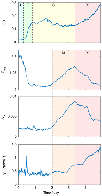
Figure 14: Four bacteria suspension parameters measured over a span of five days: (i) optical density (OD), (ii) $C_{\mathrm{mag}}$, which quantifies the ratio of magnetic to nonmagnetic bacteria, (iii) $\Delta_{\text{OD}}$, which quantifies the amount of magnetic bacteria, and (iv) $\gamma$, which quantifies how strongly the bacteria respond to magnetic fields. The following phases can be identified: lag L, exponential E, stationary S, magnetic growth M, and an undefined phase X.

IV.2.5 Marathon test: MC-1 velocity measurement

In contrast to MSR-1 bacteria, which reverse frequently, magnetotactic bacteria of type MC-1 tend to swim for long periods in the same direction [25]. This allows us to collect a large number of bacteria at the bottom of a cuvette simply by applying a vertical field. After reversing the direction of the field, all bacteria swim upward in a band-shaped cloud. In the MagOD system, the passing of this cloud translates to a drop in the photodetector signal. The time between reversal of the field and the response on the photodetector is a measure for the velocity of the bacteria. We call this method the “marathon” test.

To obtain sufficient bacteria for this experiment, we cultivated MC-1 bacteria in a high-viscosity, agarose-based medium in an oxygen gradient, as described by Bazylinski [47], but use low-melt agarose instead of bacto agar. The bacteria form a band in the reaction tube a few millimeters below the surface of the medium [48]. The easiest way to free the MC-1 from the medium is to pipette a small amount from the band and insert this into a cuvette filled with a low-viscosity growth medium from which the agarose has been omitted. The transfer of some agarose cannot be avoided, especially if large quantities of bacteria are desired.

Alternatively, one can place a droplet of agarose with bacteria on one side and a droplet of growth medium with agarose next to it so they merge. One can then use a magnet to draw the MC-1 out of the agarose and into a clean droplet. The disadvantage of this method is that only a limited amount of bacteria can be collected and that it is difficult to avoid admitting oxygen into the sample.

The method we prefer is to pass the mixture of bacteria and agarose through a Pasteur pipette filled with a small plug of cotton. Our assumption is that the cotton breaks up the agarose matrix and perhaps even captures it. By using compressed nitrogen to push the growth medium with bacteria through the plug, exposure to oxygen can be avoided. To reduce oxygen exposure even further, we performed this procedure in a nitrogen atmosphere. For this purpose, we simply use a glass beaker with a paraffin cover through which the Pasteur pipette is inserted into the cuvette.

The MagOD system is equipped with a 3D magnetic coil configuration, which makes it simple to apply a vertical field along the cuvette. A field of $1\text{\,}\mathrm{m}\mathrm{T}$ is applied in positive $z$-direction for $220\text{\,}\mathrm{s}$ to collect south-seeking bacteria at the bottom of the cuvette. Then the field is reversed so that the collected bacteria swim upward towards the photodetector. We allow the bacteria to swim upward for $200\text{\,}\mathrm{s}$, after which the sequence is repeated. The asymmetry in time ensures that a sufficient amount of bacteria can reassemble at the bottom of the cuvette. The cloud of bacteria that leaves the bottom of the cuvette disperses due to a distribution of bacteria velocities. To keep the peak sharp and intensity variation high, we reduce the distance between the bottom of the cuvette and the light path to $2.5\text{\,}\mathrm{m}\mathrm{m}$ by using a special insert.

Figure 15 shows the output of the photodetector as a function of time elapsed after the magnetic field reversal. A series of eight experiments are shown. For each experiment, the cloud reaches the light path after approximately $30\text{\,}\mathrm{s}$ with a maximum density at about $90\text{\,}\mathrm{s}$. As time progresses, the curves have a similar shape, but with a lower amplitude. Apparently, less and less bacteria collect at the bottom of the cuvette. The decrease in amplitude shown in Figure 16 agrees very well with an exponential decay $\exp(-t/\tau)$ and a time constant of approximately 30 min. This suggests that a fixed amount of bacteria is lost per iteration. The reason for the loss is yet unclear; this remains a topic for further investigation.

The arrival time $t$ (s) of MC-1 at the detector agrees well with a log-normal distribution (shown as red curves in Figure 15),

$$f_{\text{t}}(t)=\frac{1}{t\sigma\sqrt{2\pi}}\exp\left(\frac{-\left(\ln(t)-\mu\right)^{2}}{2\sigma^{2}}\right)\text{ (1/s)}\,,$$ (9)

where $\mu$ (with unit $\ln(s)$) and $\sigma$ (unitless) are the mean and standard deviation of the natural logarithm of $t$, respectively. From the distance of $2.5\text{\,}\mathrm{m}\mathrm{m}$ from the bottom of the cuvette to the light beam $a$, we can calculate the distribution of the velocities $v$ (m/s) as follows:

$$f_{\text{v}}(v)=\frac{1}{v\sigma\sqrt{2\pi}}\exp\left(\frac{-\left(\ln(\frac{a}{v})-\mu\right)^{2}}{2\sigma^{2}}\right)\text{ (s/m)}\,.$$ (10)

The most likely velocity, or mode of this distribution, is

$$v_{\text{m}}=a\exp\left(-(\mu+\sigma^{2})\right)\text{ (m/s)}\,.$$ (11)

The resulting velocity distributions are shown in the lower graph of Figure 15. The curves are offset vertically for clarity; the top curve is the first measurement. This figure shows clearly that the velocity distribution of the bacteria does not change significantly with time. As the experiment duration was limited to $200\text{\,}\mathrm{s}$, the minimum velocity that can be determined is $12.5\text{\,}\mathrm{\SIUnitSymbolMicro}\mathrm{m}\mathrm{/}\mathrm{s}$. The most likely velocity is on the order of $20\text{\,}\mathrm{\SIUnitSymbolMicro}\mathrm{m}\mathrm{/}\mathrm{s}$, and the fastest bacteria swim a rate of approximately $80\text{\,}\mathrm{\SIUnitSymbolMicro}\mathrm{m}\mathrm{/}\mathrm{s}$.

Figure 15 is a typical example; we have measured both faster and slower average velocities. The measured velocity is considerably lower than that observed by Lefèvre and colleagues using high-speed microscopy [3]. We noted from experiments with microfluidic chips that the velocity distribution is strongly dependent on the duration the MC-1 have been growing in the semi-solid medium, temperature (both too high and too low reduced velocity) and oxygen concentration. Further experiments are required to determine the relation between the velocity and these environmental conditions.

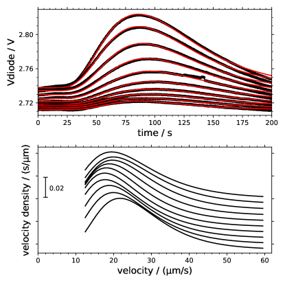
Figure 15: Photodetector output as a function of time elapsed since reversal of the magnetic field. After approximate $30\text{\,}\mathrm{s}$, the first MC-1 pass the light beam and scatter the light. Maximum light extinction is reached about $90\text{\,}\mathrm{s}$. The experiment is repeated eight times in intervals of $440\text{\,}\mathrm{s}$ between measurements. The responses fit relatively well to a log-normal distribution (red lines). These fits can be inverted to obtain the velocity distribution of the MC-1 (bottom curve). For clarity, these curves are offset by $0.005\text{\,}\mathrm{s}\mathrm{/}\mathrm{\SIUnitSymbolMicro}\mathrm{m}$ from top to bottom. The velocity distribution remains more or less constant.

Figure 16: Decrease in amplitude of the marathon curves in Figure 15 with increasing time agrees very well with an exponential decay.

V Discussion

Our novel MagOD magnetic absorbance instrument has proved to be a versatile system that can be successfully applied to research on magnetotactic bacteria. All designs and source codes have been made available online, so that the system can be easily replicated, modified and improved. The data presented in this paper is intended to serve as a benchmark for future systems. We hope our efforts will inspire colleagues to improve and apply the MagOD system for their own research. In the following, we address possible improvements and suggestions for further research.

V.1 Possible improvements

There are a few issues regarding the measurement head, measurement board and software that deserve attention for future iterations of the system.

V.1.1 Measurement head

The response of the photodiode to the blue LED is nonlinear, see Figure 5, for which we do not have a satisfactory explanation. Furthermore, the fact that the signal is inversely proportional to the light intensity is counterintuitive. It may be possible to redesign the amplifier while maintaining the required footprint. The noise floor in the current design is still a factor of 30 above the theoretical limit, and there are signs that $50\text{\,}\mathrm{H}\mathrm{z}$ crosstalk deteriorates the signal, see Figure 8. One might consider moving the AD converter from the measurement board to the measurement head to better protect the signal from interference. To compensate for drift, automatic offset correction can be applied by modulating the LED intensity periodically.

One might consider moving the LED drivers to the measurement head, so that the high-frequency PWM signal does not have to be transported over the HDMI cable. This would free up ports on the ESP32. For this purpose, RGB LED drivers that communicate over I²C are readily available. Care should be taken that the I²C clock signal does not interfere with the detection electronics.

If suspensions with higher densities are to be observed, one might consider using solid-state lasers that offer at least $100\text{\,}$ times higher light intensity.

In contrast to commercial absorbance meters, our MagOD system does not have a piezoelectric actuator to disperse the suspension prior to measurement. One might consider integrating such a component. Alternatively, one might make use of the existing coils and attempt a voice coil actuation principle using a soft magnetic element, an additional small coil or even a small permanent magnet mounted such that it does not interfere with the field.

Since we use air coils, the magnetic field is simply proportional to the current, which is measured. This works very well for fields in the order of a few mT. For fields below $1\text{\,}\mathrm{m}\mathrm{T}$, the magnetic background field (for instance the Earth magnetic field) becomes noticeable. One simple solution is to determine the background field at the location of the setup using a three-axis Hall sensor and compensate in a feed forward manner. However, the compensation needs to be recalibrated every time the setup is moved. A much more precise solution, which also corrects for soft magnetic and hard magnetic parts of the setup, was described in detail in ref [49] and is based on the determination of the magnetic response function of the setup at the predicted detection location in the sample. Since three-axis Hall sensors are routinely used in mobile phone mobile phones, there have become very small and inexpensive. Therefore they can be relatively easily positioned around the detection area. The approach by Ahlers, in combination with a feedback loop, would thus allow for very precise, realtime compensation in the $\text{\,}\mathrm{\SIUnitSymbolMicro}\mathrm{T}$ range.

V.1.2 Measurement board

In future designs of the measurement board, a number of improvements could be made as well. Even though the AD converter is capable of data acquisition at $860\text{\,}\mathrm{s}\mathrm{a}\mathrm{m}\mathrm{p}\mathrm{l}\mathrm{e}\mathrm{s}\mathrm{/}\mathrm{s}$, we achieve only $323\text{\,}\mathrm{s}\mathrm{a}\mathrm{m}\mathrm{p}\mathrm{l}\mathrm{e}\mathrm{s}\mathrm{/}\mathrm{s}$ in practice. We assume this discrepancy is caused by communication overhead that could be optimized.

The current implementation of the measurement circuits allows only for positive currents. Modifying the circuits to allow for bi-directional currents is straightforward, for instance by applying an INA266 integrated current monitor.

Finally, the small form factor of micro-SD cards poses a problem in biolab environments because they are easily lost. Removal of the SD card can be avoided if WiFi access is available, but a USB stick may be a better option.

V.1.3 Software

We expect that the software of our MagOD system will undergo the most development. In addition to improvements of the user interface, the main restriction is currently that measurement recipes are based only on feed-forward instructions, i.e. iterations of a specified amount of time, field settings and LED color. There is currently no capability to react to changes in the detected signal. For instance, it would be very useful if the LED intensity could be adjusted automatically to the absorbance of the suspension under investigation. In marathon experiments, it would be convenient if the field reversal took place at a fixed delay after the occurrence of the peak. The current recipe language definition is not capable of handling this type of feedback. We suspect a complete redesign of the software is required, taking full advantage of the EPS32 capabilities. This would be a very interesting task for a (software) engineering student.

V.2 Possible future applications

The four experiments we presented are merely a selection of the many possibilities offered by our novel MagOD system. Even without additional modification, there are numerous possible experiments to inspire future work.

V.2.1 Flagellar motion

As the MagOD system has precise field control, it allows a simple study of the relation between field strength and $C_{\text{mag}}$. It would be interesting to check whether the swimming activity of the bacteria themselves contributes to their random motion, which effectively would increase $kT$ and could explain the observed difference. For instance, it would be sufficient to measure $C_{\text{mag}}$ as a function of field before and after killing the MSR-1 (for example by exposure to intense UV light or formaldehyde).

V.2.2 Multi-color optical density

So far, we have measured the transmission through MSR-1 cultures only under green light. However, we noticed that the color of cultures changes with elapsed time. We speculate that these color changes may be caused by an increase in bacteria size and/or formation of magnetosomes. For long-term analysis as illustrated in Figure 14, it may therefore be useful to measure this at different wavelengths. The MagOD system can easily achieve this by measuring iteratively with red, green and blue LEDs. Multiple wavelengths may be combined with the addition of an indicator agent that changes its absorbance spectrum based on changed conditions.

An example of such an indicator is Resazurin, which reacts to an increase in oxygen concentration with a shift in the absorbance spectrum toward red. The ratio between the absorbance in the red and green channels could therefore be a measure of the oxygen concentration in the culture, using the blue channel for calibration.

V.2.3 Modulated light intensity

The intensity of the LEDs can be varied rapidly, as illustrated in Figure 7. One can use this modulation for differential measurements to correct for interference signals due to changes in environmental light or crosstalk on the analog signal wiring.

Modulation of the light intensity would also provide information about the photosensitivity of the bacteria. For instance, one could measure $C_{\text{mag}}$ in the red channel before and after a pulse with intense blue light.

V.2.4 Combined marathon and $C_{\text{mag}}$

We demonstrated $C_{\text{mag}}$ measurements on MSR-1 bacteria and marathon tests on MC-1 bacteria. It is straightforward to combine the marathon test with $C_{\text{mag}}$ measurements. The vertical field ($z$-direction) should then be switched between zero and, for instance, a positive value, whereas the field along the light path ($x$-direction) should be switched between zero and alternatively positive and negative values, hence $(x,z)={(0,1),(1,0),(0,1),(-1,0)}$, etc. Such an experiment might reveal whether the velocity distribution is related to a distribution of magnetosome strength as well.

V.2.5 Sedimentation

We often observed an initial increase of light transmission after loading a sample with bacteria. We therefore usually waited until the signal settled. However, there may be information to be extracted from this behavior. We suspect the increase in transmission is caused by sedimentation of debris, such as dead bacteria. If the dead bacteria contain magnetosomes, they will still rotate in the magnetic field. Therefore a measurement of $C_{\text{mag}}$ during sedimentation might provide additional information about the status of the culture.

Moreover, it is very simple to drive only one coil of the vertical coil set. In this way, one can generate field gradients that would pull magnetic debris either up or down, thus decelerating or accelerating the sedimentation process.

V.2.6 Suspensions of magnetic nanoparticles

We often use our MagOD system with a suspension of magnetic micro- and nanoparticles. This works particularly well for magnetic needles [50] and magnetic discs [51]. In principle, spherical particles should not show a change in transmission under rotation of an external field. However, magnetic particles have a tendency to form chains that align with the field, see for instance the work by Gao [52]. Angle and field-dependent transmission measurements in the MagOD could therefore provide information about the dynamic interaction between particles. Use of our MagOD system could perhaps be extended even beyond the magnetotactic research community.

VI Conclusion

We constructed a magnetic spectrophotometer (magnetic optical density meter, or MagOD) that analyzes the amount of light transmitted through a suspension of a magnetotactic bacteria in a transparent cuvette under application of a magnetic field.

Light transmission measurements with our novel MagOD system were compared with those obtained with a commercial instrument (Eppendorf BioPhotoMeter) using a dilution series of a magnetic nanoparticle suspension. The deviation between our MagOD system and the commercial instrument is less than $0.2\text{\,}$ in terms of relative absorbance for wavelengths ranging from $460\text{\,}$ to $645\text{\,}\mathrm{n}\mathrm{m}$. However, the blue channel suffers from nonlinearity and should only be used at low intensities. The dynamic range (from noise level to maximum signal) of our novel MagOD system is $88\text{\,}\mathrm{d}\mathrm{B}$ (optical density of $4.4\text{\,}$), whereas the commercial system reaches $53\text{\,}\mathrm{d}\mathrm{B}$ (optical density of $2.6\text{\,}$). In addition, our MagOD system is considerably faster, with a sample rate of $323\text{\,}\mathrm{s}\mathrm{a}\mathrm{m}\mathrm{p}\mathrm{l}\mathrm{e}\mathrm{s}\mathrm{/}\mathrm{s}$, whereas the commercial instrument has a sampling time in excess of $1\text{\,}\mathrm{s}$.

The magnetic field can be applied in three directions, with a set-point resolution of $70\text{\,}\mathrm{n}\mathrm{T}$ and a ripple of less than $50\text{\,}\mathrm{\SIUnitSymbolMicro}\mathrm{T}$. The maximum field is $5.1(1)\text{\,}\mathrm{m}\mathrm{T}$, but is limited in duration due to coil heating. When a field of $1.0\text{\,}\mathrm{m}\mathrm{T}$ is continuously applied, the temperature increase of the cuvette is approximately $1\text{\,}\mathrm{K}\mathrm{/}\mathrm{h}$ and limited to $2.1(3)\text{\,}\mathrm{K}$.

The MagOD system was used to characterize various aspects of MSR-1 and MC-1 magnetotactic bacteria. By means of the magnetic field, MSR-1 bacteria were oriented at different angles with respect to the light path. The transmission rate is high when bacteria are aligned along the light beam and lower when the bacteria are aligned perpendicular to the light path. The relation between angle and optical density can be approximated relatively well by a sine function.

The difference in transmission rates allows us to derive a measure for the amount of magnetic bacteria. This amount is commonly expressed as a ratio $C_{\text{mag}}$, which is a parameter that increases with the relative fraction of magnetic bacteria compared to the total number of bacteria. It can also be expressed as a difference $\Delta_{\text{OD}}$, which is a measure for the absolute amount of magnetic bacteria. Both parameters increase with applied field strength in a way that is in agreement within measurement error with a simple model based on Brownian motion.

We used our novel MagOD system to continuously monitor the development of a culture of MSR-1 magnetotactic bacteria for $5\text{\,}\mathrm{d}\mathrm{a}\mathrm{y}\mathrm{s}$. We recorded the optical density $O_{\text{D}}$, change in light transmission under rotation of the magnetic field $C_{\mathrm{mag}}$ and $\Delta_{\text{OD}}$, and the rotation velocity of the bacteria $\gamma$. We were able to distinguish clearly the separate growth phases (lag, exponential growth, and stationary). The increase in magnetic response $C_{\mathrm{mag}}$ and $\Delta_{\text{OD}}$ takes place during the stationary phase.

Unipolar bacteria such as MC-1 can be collected at the bottom of the cuvette with a vertical magnetic field. Upon reversal of the field, the entire group departs from the bottom and will arrive at the light beam, causing a dip in the transmitted light. This “marathon” test allows us to measure the velocity distribution.

The arrival times can be accurately described by a log-normal distribution, with a mode (most frequently occurring velocity) of $20\text{\,}\mathrm{\SIUnitSymbolMicro}\mathrm{m}\mathrm{/}\mathrm{s}$. The maximum velocity we observed is on the order of $80\text{\,}\mathrm{\SIUnitSymbolMicro}\mathrm{m}\mathrm{/}\mathrm{s}$. The amount of bacteria participating in the marathon test decreases exponentially with each test with a time constant of approximately 30 min.

The dedicated magnetic optical density meter presented here is relatively simple and inexpensive, yet the data that can be extracted from magnetotactic bacteria cultures is rich in detail. All information for the construction of the device, including 3D print designs, printed circuit board layouts and code for the microprocessor, has been made available online. The authors trust that the magnetotactic bacteria community will benefit from our work, and that the MagOD instrument will become a valuable tool for research in this field.

Supplementary Online Material

The online supplementary material contains a python script (angular.py) to numerically integrate the equations in section II.3, and a video of the LED intensity (MagODLEDProjection.mov) accompanying figure 18.

Appendix A $C^{*}_{\text{mag}}$ and $C_{\text{mag}}$ approximations

The effect of a magnetic field rotation is usually small. It is therefore useful to express the variation with respect to the average intensity or absorbance

$$I_{\text{s}}=\frac{I(0)+I(90)}{2}$$ (12)

$$A=\log(I_{\text{ref}}/I_{\text{s}})$$ (13)

by a small deviation $\alpha$

$$A(0)=(1+\alpha)A$$ (14)

$$A(90)=(1-\alpha)A$$ (15)

so that

$$\Delta_{\text{A}}=2\alpha A$$ (16)

and

$$C_{\text{mag}}=\frac{(1+\alpha)}{(1-\alpha)}\approx 1+2\alpha=1+\frac{\Delta_{\text{A}}}{A}\,.$$ (17)

The approximation is better than $5\text{\,}\mathrm{\char 37\relax}$ in terms of $C_{\text{mag}}-1$ for $C_{\text{mag}}<1.1$.

Similarly, to estimate $C^{*}_{\text{mag}}$, we can define

$$\Delta I=2\beta I_{\text{s}}$$ (18)

so that

$$C^{*}_{\text{mag}}\approx 1+\frac{I_{\text{s}}}{I_{\text{ref}}-I_{\text{s}}}2\beta=\ 1+\frac{\Delta I}{I_{\text{ref}}-I_{\text{s}}}\,.$$ (19)

Both definitions of $C_{\text{mag}}$ can be related by realizing that

$$\frac{I(0)}{I_{\text{ref}}}=\left(\frac{I_{\text{s}}}{I_{\text{ref}}}\right)^{1+\alpha}\approx\ \frac{I_{\text{s}}}{I_{\text{ref}}}\left(1+\alpha\ln(I_{\text{s}}/I_{\text{ref}})\right)$$ (20)

and similarly for $I(90)$ with $-\alpha$, so that

$$\Delta I=-2\alpha I_{\text{s}}\ln(I_{\text{s}}/I_{\text{ref}})\,.$$ (21)

Therefore, in the approximation for $C_{\text{mag}}$ close to unity, the relation between these two definitions is

$$\frac{C_{\text{mag}}-1}{C^{*}_{\text{mag}}-1}\approx\ \frac{\Delta_{\text{A}}}{A}\frac{I_{\text{ref}}-I_{\text{s}}}{\Delta I}=$$ (22)

$$\frac{I_{\text{ref}}-I_{\text{s}}}{I_{\text{s}}\ln(I_{\text{ref}}/I_{\text{s}})}=\frac{(I_{\text{ref}}-I_{s})\log(e)}{I_{\text{s}}A}.$$ (23)

The definitions converge for $I_{\text{s}}\to I_{\text{ref}}$ for samples with very low optical density.

Appendix B Arccotangent approximation

For fitting purposes, the rather complicated arccotangent expression of Eq. (7) can be approximated by a much simpler exponential function. The fit was performed in gnuplot, resulting in a fit parameter of $0.85(1)\text{\,}$. The error is less than $0.065\text{\,}\mathrm{r}\mathrm{a}\mathrm{d}$ as shown in Figure 17.

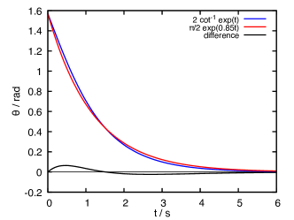
Figure 17: Approximation by an exponential function of the exact solution to the differential equation for the rotation of the bacterium as a function of time, see Eq. (7). The optimal fit is for a prefactor $0.85(1)\text{\,}$, in which case the error is less than $0.065\text{\,}\mathrm{r}\mathrm{a}\mathrm{d}$.

Appendix C Measurements

Figure 18 shows the projection onto a sheet of white paper of the light exiting from the measurement head (with the photodetector circuit board removed). The images are snapshots of a video taken with an iPhone camera for a range in LED duty cycles (measurement of Figure 19). The full video is available in the Supplementary Material, see MagODLEDprojection.mov. The opening behind the cuvette is a square hole of $3$$\times$$3\text{\,}\mathrm{m}\mathrm{m}$, which is clearly visible. The photodetector itself has an area of $2.7$$\times$$2.7\text{\,}\mathrm{m}\mathrm{m}$, hence it collects the inner portion of this pattern. For the green and blue LEDs, echo images can be observed. The three patterns do not align, which is most likely caused by the fact that the three LEDs in the WP154 housing are not centered on the axis of the front lens. From the distance between the projected image and the LED (approximately $15\text{\,}\mathrm{c}\mathrm{m}$), with a maximum shift of about $5\text{\,}\mathrm{m}\mathrm{m}$, we estimate that the misalignment is on the order of $2\text{\,}\mathrm{\SIUnitSymbolDegree}$. As the photodetector is mounted directly behind the opening behind the cuvette, this misalignment is of no consequence.

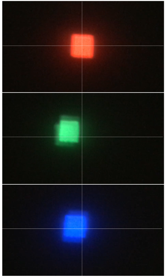
Figure 18: Projection of the light pattern of the three different LEDs. The $3$$\times$$3\text{\,}\mathrm{m}\mathrm{m}$ opening at the back of the cuvette can clearly be seen. The green and blue LEDs show some reflection, and the patterns are not aligned. The estimated misalignment is on the order of $2\text{\,}\mathrm{\SIUnitSymbolDegree}$. As the photodetector has a sensitive area of $2.7$$\times$$2.7\text{\,}\mathrm{m}\mathrm{m}$ and is mounted directly behind the opening in the holder, we expect no adverse effects from the reflections of misalignment. A full video of the pattern shape as a function of intensity is available in the Supplementary Material.

Figure 19 shows the intensity on the photodetector as a function of the duty cycle of each of the three LEDs for a cuvette filled with water and three different dilutions of a EMG304 magnetic nanoparticle suspension. The absorbance relative to the water-filled cuvette is determined from the difference in slopes. This measurement is used for the MagOD data points in Figure 6. The blue LED suffers from artefacts. The slope is not constant, but lower at high intensities. Furthermore, there is a small step at an intensity of about $0.6$. For the estimate of absorbance of the blue LED, only the linear region at low intensity was used.

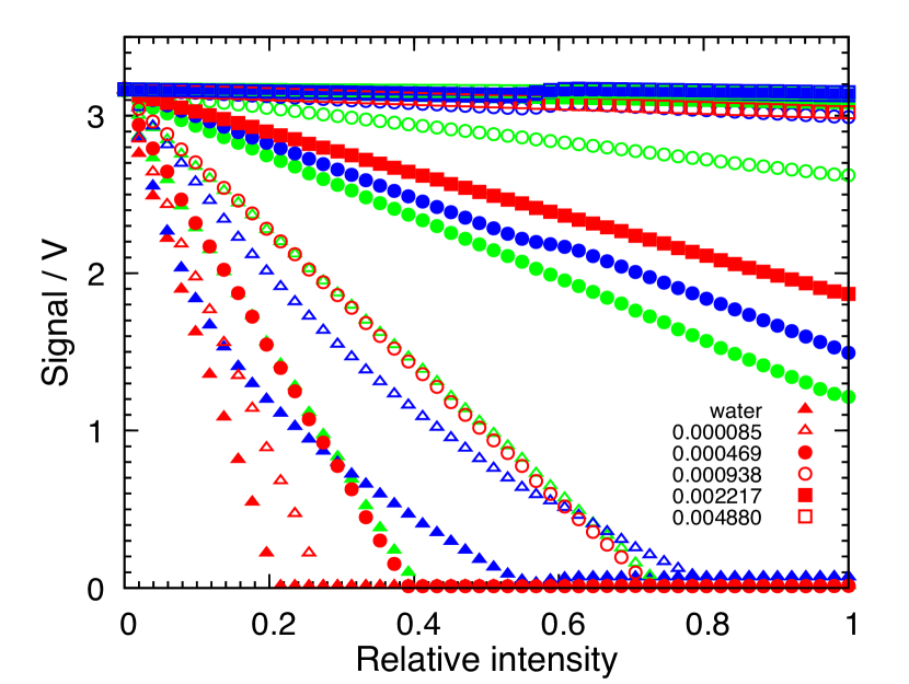
Figure 19: Signal as a function of the LED duty cycle for the three different LED wavelengths as well as for a water reference and three different dilutions of a EMG304 magnetic nanoparticle suspension.

References

- Frankel et al. [1979] R. B. Frankel, R. P. Blakemore, and R. S. Wolfe, Science 203, 1355 (1979).
- Farina et al. [1990] M. Farina, D. Esquivel, and H. De Barros, Nature 343, 256 (1990).
- Lefèvre et al. [2014] C. Lefèvre, M. Bennet, L. Landau, P. Vach, D. Pignol, D. Bazylinski, R. Frankel, S. Klumpp, and D. Faivre, Biophysical Journal 107, 527 (2014).
- Bellini [2009] S. Bellini, Chinese Journal of Oceanology and Limnology 27, 3 (2009).
- Blakemore et al. [1979] R. P. Blakemore, D. Maratea, and R. S. Wolfe, Journal of Bacteriology 140, 720 (1979).
- Lee et al. [2004] H. Lee, A. Purdon, V. Chu, and R. Westervelt, Nano Letters 4, 995 (2004).
- Khalil et al. [2013] I. S. M. Khalil, M. P. Pichel, L. Abelmann, and S. Misra, The International Journal of Robotics Research 32, 637 (2013).
- Pichel et al. [2018] M. P. Pichel, T. A. G. Hageman, I. S. M. Khalil, A. Manz, and L. Abelmann, Journal of Magnetism and Magnetic Materials 460, 340 (2018).
- Futschik et al. [1989] K. Futschik, H. Pfützner, A. Doblander, P. Schönhuber, T. Dobeneck, N. Petersen, and H. Vali, Physica Scripta 40, 518 (1989).
- Harasko et al. [1995] G. Harasko, H. Pfutzner, and K. Futschik, IEEE Transactions on Magnetics 31, 938 (1995).
- Hergt et al. [2005] R. Hergt, R. Hiergeist, M. Zeisberger, D. Schüler, U. Heyen, I. Hilger, and W. A. Kaiser, Journal of Magnetism and Magnetic Materials 293, 80 (2005).
- Gandia et al. [2019] D. Gandia, L. Gandarias, I. Rodrigo, J. Robles-García, R. Das, E. Garaio, J. Á. García, M.-H. Phan, H. Srikanth, I. Orue, J. Alonso, A. Muela, and M. L. Fdez-Gubieda, Small 15, 1902626 (2019).
- Makela et al. [2022] A. V. Makela, M. A. Schott, C. S. Madsen, E. M. Greeson, and C. H. Contag, Nano Letters 22, 4630 (2022).
- Martel and Mohammadi [2010] S. Martel and M. Mohammadi, Proceedings - IEEE International Conference on Robotics and Automation , 500 (2010).
- Martel et al. [2009] S. Martel, M. Mohammadi, O. Felfoul, Z. Lu, and P. Pouponneau, International Journal of Robotics Research 28, 571 (2009).
- Khalil et al. [2013] I. Khalil, V. Magdanz, S. Sanchez, O. Schmidt, L. Abelmann, and S. Misra, Proceedings of the Annual International Conference of the IEEE Engineering in Medicine and Biology Society, EMBS , 5299 (2013).
- De Lanauze et al. [2014] D. De Lanauze, O. Felfoul, J.-P. Turcot, M. Mohammadi, and S. Martel, International Journal of Robotics Research 33, 359 (2014).
- Felfoul et al. [2016] O. Felfoul, M. Mohammadi, S. Taherkhani, D. De Lanauze, Y. Zhong Xu, D. Loghin, S. Essa, S. Jancik, D. Houle, M. Lafleur, L. Gaboury, M. Tabrizian, N. Kaou, M. Atkin, T. Vuong, G. Batist, N. Beauchemin, D. Radzioch, and S. Martel, Nature Nanotechnology 11, 941 (2016).
- Zingsem et al. [2019] B. W. Zingsem, T. Feggeler, A. Terwey, S. Ghaisari, D. Spoddig, D. Faivre, R. Meckenstock, M. Farle, and M. Winklhofer, Nature Communications 10, 4345 (2019).
- Rosenblatt et al. [1982] C. Rosenblatt, F. F. T. de Araujo, and R. B. Frankel, Journal of Applied Physics 53, 2727 (1982).
- Faivre et al. [2010] D. Faivre, A. Fischer, I. Garcia-Rubio, G. Mastrogiacomo, and A. Gehring, Biophysical Journal 99, 1268 (2010).
- Fernández-Castané et al. [2018] A. Fernández-Castané, H. Li, O. R. Thomas, and T. W. Overton, New Biotechnology 46, 22 (2018).
- Yang et al. [2013] J. Yang, S. Li, X. Huang, T. Tang, W. Jiang, T. Zhang, and Y. Li, Frontiers in Microbiology 4, (2013).
- Song et al. [2014] T. Song, L. Zhao, and L.-F. Wu, IEEE Transactions on Magnetics 50, (2014).
- Lefèvre et al. [2009] C. Lefèvre, T. Song, J.-P. Yonnet, and L.-F. Wu, Applied and Environmental Microbiology 75, 3835 (2009).
- Chen et al. [2014] C.-Y. Chen, C.-F. Chen, Y. Yi, L.-J. Chen, L.-F. Wu, and T. Song, Biomedical Microdevices 16, 761 (2014).
- Schüler et al. [1995] D. Schüler, R. Uhl, and E. Bäuerlein, FEMS Microbiology Letters 132, 139 (1995).
- Bennet et al. [2016] M. Bennet, D. Gur, J. Yoon, Y. Park, and D. Faivre, Advanced Optical Materials 5, 1600617 (2016).
- Katzmann et al. [2013] E. Katzmann, M. Eibauer, W. Lin, Y. Pan, J. Plitzko, and D. Schuler, Applied and Environmental Microbiology 79, 7755 (2013).
- Myers et al. [2013] J. A. Myers, B. S. Curtis, and W. R. Curtis, BMC Biophysics 6, 4 (2013).
- Zhao et al. [2007] L. Zhao, D. Wu, L.-F. Wu, and T. Song, Journal of Biochemical and Biophysical Methods 70, 377 (2007).
- Lang and Schüler [2008] C. Lang and D. Schüler, Applied and Environmental Microbiology 74, 4944 (2008).
- Schüler and Baeuerlein [1998] D. Schüler and E. Baeuerlein, Journal of Bacteriology 180, 159 (1998).
- Heyen and Schüler [2003] U. Heyen and D. Schüler, Applied Microbiology and Biotechnology 61, 536 (2003).
- Esquivel and Lins de Barros [1986] D. Esquivel and H. Lins de Barros, Journal of Experimental Biology 121, 153 (1986).
- Steinberger et al. [1994] B. Steinberger, N. Petersen, H. Petermann, and D. G. Weiss, Journal of Fluid Mechanics 273, 189 (1994).
- Zahn et al. [2017] C. Zahn, S. Keller, M. Toro-Nahuelpan, P. Dorscht, W. Gross, M. Laumann, S. Gekle, W. Zimmermann, D. Schüler, and H. Kress, Scientific Reports 7, (2017).
- Erglis et al. [2007] K. Erglis, Q. Wen, V. Ose, A. Zeltins, A. Sharipo, P. A. Janmey, and A. Cebers, Biophysical Journal 93, 1402 (2007).
- Pan et al. [2009] Y. Pan, W. Lin, J. Li, W. Wu, L. Tian, C. Deng, Q. Liu, R. Zhu, M. Winklhofer, and N. Petersen, Biophysical Journal 97, 986 (2009).
- Lane et al. [2001] J. E. Lane, R. C. Youngquist, C. D. Immer, and J. C. Simpson, National Aeronautics and Space Administration, Washington , 217918 (2001).
- Hergert [2014] E. Hergert, Guide to Detector Selection, Tech. Rep. (Hamamatsu Cooperation, 2014).
- Pfeiffer and Schüler [2020] D. Pfeiffer and D. Schüler, Applied and Environmental Microbiology 86, 10.1128/aem.01976-19 (2020).
- Popp et al. [2014] F. Popp, J. Armitage, and D. Schüler, Nature Communications 5, (2014).
- Staniland et al. [2010] S. S. Staniland, C. Moisescu, and L. G. Benning, Journal of Basic Microbiology 50, 392 (2010).
- Yang et al. [2001] C.-D. Yang, H. Takeyama, T. Tanaka, A. Hasegawa, and T. Matsunaga, Applied Biochemistry and Biotechnology 91-93, 155 (2001).
- Pichel [2018] M. Pichel, The behavior of magnetotacticbacteria in changing magnetic fields, Ph.D. thesis, University of Twente (2018).
- Bazylinski et al. [2013] D. A. Bazylinski, T. J. Williams, C. T. Lefèvre, R. J. Berg, C. L. Zhang, S. S. Bowser, A. J. Dean, and T. J. Beveridge, International Journal of Systematic and Evolutionary Microbiology 63, 801 (2013).
- Lefèvre et al. [2016] C. T. Lefèvre, P. A. Howse, M. L. Schmidt, M. Sabaty, N. Menguy, G. W. Luther, and D. A. Bazylinski, Environmental Microbiology Reports 8, 1003 (2016).
- Ahlers et al. [2022] M. T. Ahlers, C. T. Block, M. Winklhofer, and M. Greschner, PLOS ONE 17, e0271765 (2022).
- Song et al. [2021] S.-H. Song, J. Yoon, Y. Jeong, Y.-G. Jung, L. Abelmann, and W. Park, Journal of Magnetism and Magnetic Materials 539, 168341 (2021).
- Löthman et al. [2018] P. Löthman, T. Hageman, J. Hendrix, H. Keizer, H. van Wolferen, K. Ma, M. van de Loosdrecht, B. ten Haken, T. Bolhuis, and L. Abelmann, 8th International Workshop on Magnetic Particle Imaging (2018).
- Gao et al. [2013] Y. Gao, A. van Reenen, M. A. Hulsen, A. M. de Jong, M. W. J. Prins, and J. M. J. den Toonder, Lab on a Chip 13, 1394 (2013).