Comparative study of ${}^{6}{\rm He}$ $\beta$-decay based on different similarity-renormalization-group-evolved chiral interactions

Abstract

We report on a study of the Gamow-Teller matrix element contributing to ${}^{6}{\rm He}$ $\beta$-decay with similarity renormalization group (SRG) versions of momentum- and configuration-space two-nucleon interactions. These interactions are derived from two different formulations of chiral effective field theory ($\chi$EFT)—without and with the explicit inclusion of $\Delta$-isobars. We consider evolution parameters $\Lambda_{\rm SRG}$ in the range between 1.2 and 2.0 fm^-1 and, for the $\Delta$-less case, also the unevolved (bare) interaction. The axial current contains one- and two-body terms, consistently derived at tree level (no loops) in the two distinct $\chi$EFT formulations we have adopted here. The ${}^{6}{\rm He}$ and ${}^{6}{\rm Li}$ ground-state wave functions are obtained from hyperspherical-harmonics (HH) solutions of the nuclear many-body problem. In $A\,$=$\,6$ systems, the HH method is limited at present to treat only two-body interactions and non-SRG evolved currents. Our results exhibit a significant dependence on $\Lambda_{\text{SRG}}$ of the contributions associated with two-body currents, suggesting that a consistent SRG-evolution of these is needed in order to obtain reliable estimates. We also show that the contributions from one-pion-exchange currents depend strongly on the model (chiral) interactions and on the momentum- or configuration-space cutoffs used to regularize them. These results might prove helpful in clarifying the origin of the sign difference recently found in No-Core-Shell-Model and Quantum Monte Carlo calculations of the ${}^{6}{\rm He}$ Gamow-Teller matrix element.

I Introduction

Nuclear $\beta$ decays have become, in recent years, a research topic of intense interest. A quantitative understanding of these decays is crucial for a number of experimental endeavors, including the program of experiments planned at the Facility for Rare Isotope Beams (FRIB) to measure weak-interaction rates in nuclei, and neutrinoless double-$\beta$ decay experiments aimed at establishing the Dirac or Majorana nature of the neutrino. In this context, of particular relevance are Gamow-Teller matrix elements (GTMEs). Shell-model calculations have typically failed to reproduce the measured values of these, unless an effective (one-body) Gamow-Teller (GT) operator is used with a nucleon axial coupling constant $g_{A}$ that is quenched by about $20$–30% relative to its free value Chou et al. (1993); Engel and Menéndez (2017). The shell model also yields rather uncertain estimates Engel and Menéndez (2017) for the nuclear matrix elements entering neutrinoless double-$\beta$ decay rates, which are proportional to $g_{A}^{4}$. Therefore an understanding of the origin of $g_{A}$-quenching is important, as is a reliable estimate of the contributions from many-body terms in the weak current.

There have been indications Pastore et al. (2018); Gysbers et al. (2019); King et al. (2020) that $g_{A}$ quenching might originate from lack of correlations in shell-model wave functions, and possibly from two-body axial current contributions that tend to decrease the matrix element calculated with the leading one-body GT operator Gysbers et al. (2019). In this context, it is interesting to note that the Gysbers et al. study Gysbers et al. (2019) consistently finds these two-body contributions to generally have the opposite sign relative to the leading GT contributions in nuclei with mass number $A>3$. This is in contrast to the results of Refs. Pastore et al. (2018); King et al. (2020), in which the sign of the one- and two-body contributions is the same, at least in light nuclei with mass number $A\leq 10$, the only ones accessible at this time to Green’s function Monte Carlo (GFMC) methods. The origin of this difference is yet to be clarified. Of course, the comparison of results obtained by different groups is difficult owing to the different models adopted to describe nuclear interactions, and the different methods used to solve the nuclear quantum many-body problem. At this point in time, what can be stated with confidence is that Gysbergs et al. Gysbers et al. (2019) and the authors of Refs. Pastore et al. (2018); King et al. (2020) only agree on the magnitude of the two-body corrections: they are small in the $A\leq 10$ mass range.

In this work, in an attempt to understand the origin of this discrepancy, we present a calculation of the GTME contributing to the $\beta$-decay of ${}^{6}{\rm He}$, within the hyperspherical-harmonics (HH) method developed by the Pisa group Kievsky et al. (2008); Marcucci et al. (2020), and recently extended to deal with $A\,$=$\,6$ nuclei Gnech et al. (2020). The ${}^{6}{\rm He}$ and ${}^{6}{\rm Li}$ wave functions are obtained from a Hamiltonian including two-nucleon ($2N$) interactions only. Three-nucleon ($3N$) interactions are neglected, since it is not yet possible to incorporate them in HH calculations of $A\,$=$\,6$ nuclei (although some progress in this direction has been recently made, see Ref. Schiavilla et al. (2021), by including the $3N$ contact interaction that enters pionless effective field theory at leading order).

We adopt $2N$ interactions obtained in two different formulations of $\chi$EFT: one Entem et al. (2017) includes pions and nucleons as degrees of freedom, while the other Piarulli et al. (2015, 2016) also includes $\Delta$-isobars. To each of these, we apply the similarity renormalization group (SRG) unitary transformation Bogner et al. (2007) in order to accelerate the convergence rate of the HH expansion. In reference to the nuclear axial currents, we use the chiral models of Refs. Baroni et al. (2016) and Baroni et al. (2018) in conjunction with the $\Delta$-less and $\Delta$-full interactions, respectively. These currents are treated without applying the proper SRG transformations. Clearly, the absence of both $3N$ interactions and the proper SRG-evolution of interactions and currents does not allow us to obtain a complete and fully consistent description of the process. Nevertheless, having an independent method that can deal with different interactions could prove helpful in clarifying the origin of some of the tensions mentioned above.

The main goal of the present work is to understand the origin of the difference in sign obtained for the two-body contributions to the GTME of ${}^{6}{\rm He}$ $\beta$-decay in the no-core shell model (NCSM) and GFMC calculations, reported in Ref. Gysbers et al. (2019) and Refs. Pastore et al. (2018); King et al. (2020), respectively. Since use of the next-to-next-to-leading-order (N2LO450) interaction of Ref. Entem et al. (2017) allows us to achieve a satisfactory convergence in the $A\,$=$\,6$ HH calculation even without implementing the SRG transformation, we are also in a position to assess the impact of the SRG evolution itself on the GTME, at least as it relates to the $2N$ interaction. However, we should note that the $2N$ interaction adopted here and in the study of Ref. Gysbers et al. (2019) are not the same; specifically, the authors of that work use the next-to-next-to-next-to-next-to-leading-order (N4LO500) rather than the N2LO450 model of Ref. Entem et al. (2017). The former is of higher order (N4LO versus N2LO) in the power counting and has a slightly larger cutoff (500 MeV) than the latter (450 MeV).

The other $2N$ interaction we and the authors of Ref. King et al. (2020) use in the GTME calculations is the NV2-Ia model of Ref. Piarulli et al. (2016). For this interaction, however, in order to reach convergence in the HH expansion, we are forced to implement the SRG transformation. We consider four different values for the evolution parameter $\Lambda_{\text{SRG}}$, namely $\Lambda_{\text{SRG}}\,$=$\,1.2$, 1.5, 1.8, and 2.0 fm^-1. This allows us to disentangle how two-body axial-current contributions are affected by the input $2N$ interaction model (whether N2LO450 or NV-Ia) and by the corresponding SRG-evolved versions of these models.

The paper is organized as follows. In Secs. II and III we provide a concise review of, respectively, interactions and axial currents, and the HH approach for $A\,$=$\,6$ nuclei. We report our results in Sec. IV, and close in Sec. V with some concluding remarks. A number of more technical issues having to do with the convergence of the HH method for the ${}^{6}{\rm Li}$ and the ${}^{6}{\rm He}$ ground states are relegated to Appendices A and B.

II Interactions and axial currents

In this work we use two different $2N$ chiral interactions. The first one is the next-to-next-to-leading-order (N2LO) model by Entem, Machleidt and Nosyk Entem et al. (2017). This interaction is derived from a $\chi$EFT including pions and nucleons as degrees of freedom. It is regularized in momentum space (with a cutoff $\Lambda\,$=$\,450$ MeV), and is strongly non-local in configuration space.

The second interaction is the next-to-next-to-next-to-leading-order (N3LO) model developed in Refs. Piarulli et al. (2015, 2016), which includes, in addition to pion and nucleon, $\Delta$-isobar degrees of freedom. It is formulated in configuration space and is regularized in this space with two regulators, one ($R_{S}$) for the short-range components associated with $2N$ contact terms, and the other ($R_{L}$) for the long-range ones induced by one- and two-pion exchange. Various combinations of $R_{S}$ and $R_{L}$ regulators are available, but in this work we have selected the model denoted as NV2-Ia with $(R_{S},R_{L})\,$=$\,(0.8,\!1.2)$ fm.

Below, we will refer to these two interactions as the E and P models by the initial of the first author on the relevant publications, respectively Ref. Entem et al. (2017) and Piarulli et al. (2015). Both models are evolved using the SRG unitary transformation Bogner et al. (2007), in order to improve the convergence of the HH calculation. This SRG evolution leads to momentum-space interactions which are transformed back to coordinate space by standard Fourier transforms. The matrix elements are then computed using the procedure of Ref. Gnech et al. (2020).

Since one of our goals is to understand the effect of these SRG-evolved interactions on the GTME, we consider four different values for the evolution parameter $\Lambda_{\rm SRG}$, namely, $\Lambda_{\rm SRG}\,$=$\,1.2$, 1.5, 1.8, 2.0 fm^-1. Furthermore, it has been possible with the E interaction to obtain reasonable convergence without implementing any SRG evolution (that is, with the “bare” interaction). This has allowed us to compare directly the bare and SRG calculated GTME, and to assess the role of SRG evolution on this observable (see below). However, we do not account for $3N$ interactions, since SRG evolution for these is not yet available.

Accompanying each of these interactions is a set of N3LO axial currents derived consistently in $\chi$EFT—the formulation that includes pions and nucleons for the E model, and that with, in addition, $\Delta$ isobars for the P model. We provide below their configuration-space expressions in the limit of vanishing momentum transfer of interest here:

• The leading-order (LO) term consists of the Gamow-Teller operator

  $${\bf A}^{\rm LO}_{i,a}=-\frac{g_{A}}{2}\,\tau_{i,a}\,{\bm{\sigma}}_{i}\ ,$$ (1)

  and scales, in a two-body system, as $Q^{-3}$ in the power counting—here, $Q$ denotes generically a low-momentum scale;

• The N2LO terms (scaling as $Q^{-1}$) consist of a relativistic correction to the Gamow-Teller operator

  $${\bf A}^{\rm N2LO}_{i,a}({\rm RC})=\frac{g_{A}}{4\,m^{2}}\,\tau_{i,a}\,{\bf p}_{i}\times\left({\bm{\sigma}}_{i}\times{\bf p}_{i}\right)\ ,$$ (2)

  and of a two-body operator induced by a $\Delta$-isobar intermediate state (this only enters the calculations based on the P interaction)

  $${\bf A}^{\rm N2LO}_{ij,a}(\Delta) = -\left({\bm{\tau}}_{i}\times{\bm{\tau}}_{j}\right)_{a}\left[I_{1}(r_{ij};\alpha_{1}^{\Delta})\,{\bm{\sigma}}_{i}\times{\bm{\sigma}}_{j}+I_{2}(r_{ij};\alpha_{1}^{\Delta})\,{\bm{\sigma}}_{i}\times\hat{\bf r}_{ij}\,\,{\bm{\sigma}}_{j}\cdot\hat{\bf r}_{ij}\right]$$ (3)

  $$-\tau_{j,a}\left[I_{1}(r_{ij};\alpha_{2}^{\Delta})\,{\bm{\sigma}}_{j}+I_{2}(r_{ij};\alpha_{2}^{\Delta})\,\hat{\bf r}_{ij}\,\,{\bm{\sigma}}_{j}\cdot\hat{\bf r}_{ij}\right]+(i\rightleftharpoons j)\ ;$$

• The N3LO terms (scaling as $Q^{0}$) consist of a two-body operator associated with one-pion exchange (OPE)

  $${\bf A}^{\rm N3LO}_{ij,a}({\rm OPE}) = -\left({\bm{\tau}}_{i}\times{\bm{\tau}}_{j}\right)_{a}\left[I_{1}(r_{ij};\alpha_{1})\,{\bm{\sigma}}_{i}\times{\bm{\sigma}}_{j}+I_{2}(r_{ij};\alpha_{1})\,{\bm{\sigma}}_{i}\times\hat{\bf r}_{ij}\,\,{\bm{\sigma}}_{j}\cdot\hat{\bf r}_{ij}\right]$$

  $$-\tau_{j,a}\left[I_{1}(r_{ij};\alpha_{2})\,{\bm{\sigma}}_{j}+I_{2}(r_{ij};\alpha_{2})\,\hat{\bf r}_{ij}\,\,{\bm{\sigma}}_{j}\cdot\hat{\bf r}_{ij}\right]-\left({\bm{\tau}}_{i}\times{\bm{\tau}}_{j}\right)_{a}\,\frac{1}{2}\left\{{\bf p}_{i}\,\,,\,\,\widetilde{I}(r_{ij};\widetilde{\alpha})\,{\bm{\sigma}}_{j}\cdot\hat{\bf r}_{ij}\right\}+(i\rightleftharpoons j)\ ,$$

  and of a two-body contact operator

  $${\bf A}^{\rm N3LO}_{ij,a}({\rm CT})=I_{c}(r_{ij};z_{0})\,\left({\bm{\tau}}_{i}\times{\bm{\tau}}_{j}\right)_{a}\,\left({\bm{\sigma}}_{i}\times{\bm{\sigma}}_{j}\right)\ .$$ (5)

In Eqs. (1)–(5), ${\bf p}_{k}\,$=$\,-i\,{\bm{\nabla}}_{k}$, ${\bm{\sigma}}_{k}$, and ${\bm{\tau}}_{k}$ are the momentum operator, and Pauli spin and isospin operators of nucleon $k$, respectively, $\left\{\dots\,,\,\dots\right\}$ denotes the anticommutator, and ${\bf r}_{ij}={\bf r}_{i}-{\bf r}_{j}$. Charge-raising ($+$) or charge-lowering ($-$) currents follow from ${\bf A}_{\pm}={\bf A}_{x}\pm i\,{\bf A}_{y}$, where the subscript specifies the isospin component. In a many-body system, the one-body operators above are summed over the nucleons $\sum_{i}{\bf A}_{i,a}$, while the two-body ones over the nucleon pairs $\sum_{i<j}{\bf A}_{ij,a}$.

The correlation functions entering the OPE and CT currents and corresponding to the E interaction are regularized by a momentum space cutoff given by $C_{\Lambda}(k)={\rm e}^{-(k/\Lambda)^{4}}$. They can be written as

$$I^{\rm E}_{1}(r;\alpha_{i}^{\rm E}) = -\frac{\alpha_{i}^{\rm E}}{\Lambda r}\int_{0}^{\infty}dx\,\frac{x^{3}}{x^{2}+(m_{\pi}/\Lambda)^{\,2}}\,{\rm e}^{-x^{4}}\,j_{1}(x\Lambda r)\ ,$$ (6)

$$I^{\rm E}_{2}(r;\alpha^{\rm E}_{i}) = \alpha_{i}^{\rm E}\int_{0}^{\infty}dx\,\frac{x^{4}}{x^{2}+(m_{\pi}/\Lambda)^{\,2}}\,{\rm e}^{-x^{4}}\,j_{2}(x\Lambda r)\ ,$$ (7)

$$\widetilde{I}^{\rm E}(r;\widetilde{\alpha}^{\rm\,E}) = -\widetilde{\alpha}^{\,{\rm E}}\int_{0}^{\infty}dx\,\frac{x^{3}}{x^{2}+(m_{\pi}/\Lambda)^{\,2}}\,{\rm e}^{-x^{4}}\,j_{1}(x\Lambda r)\ ,$$ (8)

$$I^{E}_{c}(r;z^{\rm E}_{0}) = z^{\rm E}_{0}\,\frac{\Lambda^{3}}{2\pi^{2}}\int_{0}^{\infty}dx\,x^{2}\,{\rm e}^{-x^{4}}\,j_{0}(x\Lambda r)\ ,$$ (9)

where the $j_{n}(z)$ are spherical Bessel functions, the $\alpha^{\rm E}_{i}$ and $\widetilde{\alpha}^{\rm\,E}$ denote the combinations of coupling constants defined as

$$\alpha_{1}^{\rm E}=\frac{\Lambda^{3}}{4\,\pi^{2}}\,\frac{g_{A}}{{f}_{\pi}^{\,2}}\left({c}_{4}+\frac{1}{4\,{m}}\right)\ ,\qquad\alpha_{2}^{\rm E}=\frac{\Lambda^{3}}{2\pi^{2}}\,\frac{g_{A}\,c_{3}}{{f}_{\pi}^{\,2}}\ ,\qquad\widetilde{\alpha}^{\rm\,E}=\frac{\Lambda^{2}}{8\,\pi^{2}}\,\frac{g_{A}}{{m}\,{f}_{\pi}^{\,2}}\ ,$$ (10)

and $z^{\rm E}_{0}$ is the low-energy constant (LEC) that characterizes the contact axial current (its determination is discussed below); note that the $\alpha^{\rm E}_{i}$ are adimensional. Here, $g_{A}$ is the nucleon axial coupling constant ($g_{A}\,$=$\,1.2723$), $f_{\pi}$ is the pion-decay constant ($f_{\pi}\,$=$\,92.4$ MeV), and $m_{\pi}$ and $m$ are the pion and nucleon masses, respectively. The values of the LECs $c_{3}$ and $c_{4}$ depend on the interaction model (either E or P) and are listed in Table 1.

	E-model	P-model
$c_{3}$	$-3.61$	$-0.79$
$c_{4}$	$\phantom{-}2.64$	$\phantom{-}1.33$

Table 1: Values of the LECs $c_{3}$ and $c_{4}$ associated with the E Entem et al. (2017) and P Piarulli et al. (2015) chiral interactions and used in the accompanying axial currents; they are in units of GeV^-1. These values are obtained from fits to $\pi N$ data without (E-model) and with (P-model) the inclusion of $\Delta$-isobars.

The (regularized) correlation functions entering the $\Delta$, OPE, and CT currents and corresponding to the P interaction are

$$I^{\rm P}_{1}(r;\alpha_{i}^{\rm P}) = -\alpha_{i}^{\rm P}\,(1+\mu)\,\frac{e^{-\mu}}{\mu^{3}}\,C_{R_{L}}(r)\ ,$$ (11)

$$I^{\rm P}_{2}(r;\alpha_{i}^{\rm P}) = \alpha_{i}^{\rm P}\,(3+3\,\mu+\mu^{2})\,\frac{e^{-\mu}}{\mu^{3}}\,C_{R_{L}}(r)\ ,$$ (12)

$$\widetilde{I}^{\rm\,P}(r;\widetilde{\alpha}^{\rm\,P}) = -\widetilde{\alpha}^{\rm\,P}\,(1+\mu)\,\frac{e^{-\mu}}{\mu^{2}}\,C_{R_{L}}(r)\ ,$$ (13)

$$I^{P}_{c}(r;z^{\rm P}_{0}) = z^{\rm P}_{0}\,\frac{1}{\pi^{3/2}\,R_{S}^{3}}\,{\rm e}^{-(r/R_{S})^{2}}\ ,$$ (14)

where $\mu\,$=$\,m_{\pi}r$, and

$$C_{R_{L}}(r)=1-\frac{1}{(r/R_{L})^{s}\,{\rm e}^{(r-R_{L})/a_{L}}+1}\ .$$ (15)

Here, $a_{L}\,$=$\,R_{L}/2$, and the exponent $s$ is taken as $s\,$=$\,6$. The $R_{S}$ and $R_{L}$ values are $(R_{S},R_{L})\,$=$\,(0.8,\!1.2)$ fm, consistently with the P model for the nuclear interaction. The correlation functions entering the $\Delta$-current of Eq. (3) are the same as Eqs. (11) and (12) but with $\alpha_{i}^{P}\rightarrow\alpha_{i}^{\Delta}$. The $\alpha_{i}^{\Delta}$ and $\alpha_{i}^{\rm P}$ combinations are defined as

$$\alpha_{1}^{\Delta} = \frac{g_{A}}{8\,\pi}\,\frac{m_{\pi}^{3}}{f_{\pi}^{2}}\,c_{4}^{\Delta}\ ,\qquad\qquad\qquad\alpha_{2}^{\Delta}=\frac{g_{A}}{4\,\pi}\,\frac{m_{\pi}^{3}}{f_{\pi}^{2}}\,c_{3}^{\Delta}\ ,$$ (16)

$$\alpha^{\rm P}_{1} = \frac{g_{A}}{8\,\pi}\,\frac{m_{\pi}^{3}}{f_{\pi}^{2}}\left(c_{4}+\frac{1}{4\,m}\right)\ ,\qquad\alpha^{\rm P}_{2}=\frac{g_{A}}{4\,\pi}\,\frac{m_{\pi}^{3}}{f_{\pi}^{2}}\,c_{3}\ ,\qquad\widetilde{\alpha}^{\rm\,P}=\frac{g_{A}}{16\,\pi}\,\frac{m_{\pi}^{2}}{m\,f_{\pi}^{2}}\ ,$$ (17)

with the LECs $c_{3}^{\Delta}$ and $c_{4}^{\Delta}$ given by

$$c_{3}^{\Delta}=-\frac{h_{A}^{2}}{9\,m_{\Delta N}}\ ,\qquad c_{4}^{\Delta}=\frac{h_{A}^{2}}{18\,m_{\Delta N}}\ ,$$ (18)

where $h_{A}$ is the nucleon-to-$\Delta$ axial coupling constant ($h_{A}\,$=$\,2.74$) and $m_{\Delta N}$ is the $\Delta$-nucleon mass difference ($m_{\Delta N}\,$=$\,293.1$ MeV).

Model	LO	N2LO+N3LO(OPE)	N3LO(CT)	$z_{0}$ [fm3]
E-SRG1.2	0.9722	$-$0.0121	$-$0.0090	0.1104
E-SRG1.5	0.9666	$-$0.0095	$-$0.0060	0.0610
E-SRG1.8	0.9606	$-$0.0053	$-$0.0042	0.0392
E-SRG2.0	0.9572	$-$0.0021	$-$0.0041	0.0370
E-bare	0.9446	0.0086	$-$0.0021	0.0193
P-SRG1.2	0.9728	0.0118	$-$0.0335	0.4665
P-SRG1.5	0.9679	0.0182	$-$0.0348	0.3963
P-SRG1.8	0.9620	0.0253	$-$0.0363	0.3843
P-SRG2.0	0.9584	0.0294	$-$0.0368	0.3764

Table 2: Results for the GTME of the tritium $\beta$-decay for the different components of the currents. Columns labeled LO, and N3LO(CT) refer to the contributions given by the axial currents of Eqs. (1), and (5), respectively; the column labeled N2LO+N3LO(OPE) refers to the cumulative contribution of the axial currents of Eqs. (2), (• ‣ II), and (3) in the P-model case. The N3LO(CT) cotribution is determined by fitting the LEC $z_{0}$, used in Eqs. (9) and (14), to reproduce the observed $\beta$-decay GTME of tritium, $\langle GT\rangle_{\rm exp}/\sqrt{3}=0.9511\pm 0.0013$ Baroni et al. (2016). The calculated values of the LEC $z_{0}$ in fm³ are reported as well in the last column of the table.

Finally, as per the determination of $z_{0}$, we note that this LEC is related to the LEC $c_{D}$ that appears in the $3N$ contact interaction Baroni et al. (2018). Since $3N$ interactions are altogether ignored in the present work, we fix directly $z_{0}$ so as to reproduce the experimental value of the GTME in tritium $\beta$-decay, $\langle GT\rangle_{\rm exp}/\sqrt{3}=0.9511\pm 0.0013$ Baroni et al. (2016), without concerning ourselves with the connection between $z_{0}$ and $c_{D}$. We do so for each of the SRG-evolved interactions corresponding to the E and P models. The numerical results for the GTME in tritium $\beta$-decay and the fitted values of $z_{0}$ are reported in Table 2.

III The Hyperspherical Harmonic method

The ${}^{6}{\rm Li}$ and ${}^{6}{\rm He}$ wave functions have been expanded using the HH basis. As reference set of Jacobi vectors for six equal-mass particles we use

$$\boldsymbol{\xi}_{1p} =\sqrt{\frac{5}{3}}\left(\boldsymbol{r}_{n}-\frac{\boldsymbol{r}_{m}+\boldsymbol{r}_{l}+\boldsymbol{r}_{k}+\boldsymbol{r}_{j}+\boldsymbol{r}_{i}}{5}\right)\ ,$$ (19)

$$\boldsymbol{\xi}_{2p} =\sqrt{\frac{8}{5}}\left(\boldsymbol{r}_{m}-\frac{\boldsymbol{r}_{l}+\boldsymbol{r}_{k}+\boldsymbol{r}_{j}+\boldsymbol{r}_{i}}{4}\right)\ ,$$

$$\boldsymbol{\xi}_{3p} =\sqrt{\frac{3}{2}}\left(\boldsymbol{r}_{l}-\frac{\boldsymbol{r}_{k}+\boldsymbol{r}_{j}+\boldsymbol{r}_{i}}{3}\right)\ ,$$

$$\boldsymbol{\xi}_{4p} =\sqrt{\frac{4}{3}}\left(\boldsymbol{r}_{k}-\frac{\boldsymbol{r}_{j}+\boldsymbol{r}_{i}}{2}\right)\ ,$$

$$\boldsymbol{\xi}_{5p} =\boldsymbol{r}_{j}-\boldsymbol{r}_{i}\ ,$$

where $(i,j,k,l,m,n)$ indicates a generic permutation $p$ of the particles. By convention, $p=1$ is chosen to correspond to $(1,2,3,4,5,6)$. For a given choice of the Jacobi vectors, the hyperspherical coordinates are given by the hyperradius $\rho$, which is independent on the permutation $p$ of the particles and is defined as

$$\rho=\sqrt{\sum_{i=1,N}\xi_{ip}^{2}}\,,$$ (20)

and by a set of variables, which in the Zernike and Brinkman representation Zernike and Brinkman (1935); de la Ripelle (1983), are the polar angles $\hat{\xi}_{ip}=(\theta_{ip},\phi_{ip})$ of each Jacobi vector and the four additional “hyperspherical” angles $\varphi_{jp}$, with $j=2,\dots,5$, defined as

$$\cos\varphi_{jp}=\frac{\xi_{jp}}{\sqrt{\xi_{1p}^{2}+\dots+\xi_{jp}^{2}}}\ .$$ (21)

Here, $\xi_{jp}$ is the magnitude of the Jacobi vector $\boldsymbol{\xi}_{jp}$. The set of variables $\hat{\xi}_{1p},\dots,\hat{\xi}_{5p},\varphi_{2p},\dots,\varphi_{5p}$ is denoted hereafter as $\Omega_{p}$. The expression of the generic $A=6$ HH function is

$${\cal Y}^{KLM}_{\mu}(\Omega_{p}) =\big{[}(((Y_{\ell_{1}}(\hat{\xi}_{1p})Y_{\ell_{2}}(\hat{\xi}_{2p}))_{L_{2}}Y_{\ell_{3}}(\hat{\xi}_{3p}))_{L_{3}}Y_{\ell_{4}}(\hat{\xi}_{4p}))_{L_{4}}Y_{\ell_{5}}(\hat{\xi}_{5p})\big{]}_{LM}$$ (22)

$$\times{\cal P}^{\ell_{1},\ell_{2},\ell_{3},\ell_{4},\ell_{5}}_{n_{2},n_{3},n_{4},n_{5}}(\varphi_{2p},\varphi_{3p},\varphi_{4p},\varphi_{5p})\,,$$

where

$${\cal P}^{\ell_{1},\ell_{2},\ell_{3}.\ell_{4},\ell_{5}}_{n_{2},n_{3},n_{4},n_{5}}(\varphi_{2p},\varphi_{3p},\varphi_{4p},\varphi_{5p})$$ (23)

$$={\cal N}_{n_{2}}^{\ell_{2},\nu_{2}}(\cos\varphi_{2p})^{\ell_{2}}(\sin\varphi_{2p})^{\ell_{1}}P_{n_{2}}^{\ell_{1}+1/2,\ell_{2}+1/2}(\cos 2\varphi_{2p})$$

$$\times{\cal N}_{n_{3}}^{\ell_{3},\nu_{3}}(\cos\varphi_{3p})^{\ell_{3}}(\sin\varphi_{3p})^{K_{2}}P_{n_{3}}^{\nu_{2},\ell_{3}+1/2}(\cos 2\varphi_{3p})$$

$$\times{\cal N}_{n_{4}}^{\ell_{4},\nu_{4}}(\cos\varphi_{4p})^{\ell_{4}}(\sin\varphi_{4p})^{K_{3}}P_{n_{4}}^{\nu_{3},\ell_{4}+1/2}(\cos 2\varphi_{4p})$$

$$\times{\cal N}_{n_{5}}^{\ell_{5},\nu_{5}}(\cos\varphi_{5p})^{\ell_{5}}(\sin\varphi_{5p})^{K_{4}}P_{n_{5}}^{\nu_{4},\ell_{5}+1/2}(\cos 2\varphi_{5p})\ ,$$

and $P^{a,b}_{n}$ are Jacobi polynomials. The coefficients ${\cal N}_{n_{j}}^{\ell_{j},\nu_{j}}$ are normalization factors given explicitly by

$${\cal N}^{\ell_{j},\nu_{j}}_{n_{j}}=\biggl{[}{2\nu_{j}\Gamma(\nu_{j}-n_{j})n_{j}!\over\Gamma(\nu_{j}-n_{j}-\ell_{j}-{1\over 2})\Gamma(n_{j}+\ell_{j}+{3\over 2})}\biggr{]}^{1/2}\,,$$ (24)

and we have defined

$$K_{j}=\ell_{j}+2n_{j}+K_{j-1}\,,\qquad\nu_{j}=K_{j}+\frac{3}{2}j-1\,,$$ (25)

with $K_{1}=\ell_{1}$ and $K_{5}=K$. The integer index $\mu$ labels the set of hyperangular quantum numbers, namely

$$\mu\equiv\{\ell_{1},\ell_{2},\ell_{3},\ell_{4},\ell_{5},L_{2},L_{3},L_{4},n_{2},n_{3},n_{4},n_{5}\}\ .$$ (26)

The wave function is constructed to have a well-defined total angular momentum $J$ and third component $J_{z}$, parity $\pi$ and isospin $T$ (in the following, we ignore the small admixtures between isospin states induced by isospin-symmetry-breaking interactions). Therefore, a complete basis of antisymmetrical hyperangular-spin-isospin states is constructed as follows

$$\Psi^{KLSTJ\pi}_{\alpha}=\sum_{p=1}^{360}\Phi^{KLSTJ\pi}_{\alpha}(i,j,k,l,m,n)\ ,$$ (27)

where the sum is over the 360 even permutations $p$ of the particles and

$$\Phi^{KLSTJ\pi}_{\alpha}(i,j,k,l,m,n)=\big{\{}{\cal Y}^{KLM}_{\mu}(\Omega_{p})[[[s_{i}s_{j}]_{S_{2}}s_{k}]_{S_{3}}$$ (28)

$$\quad\times[[s_{l}s_{m}]_{S_{4}}s_{n}]_{S_{5}}]_{S}\big{\}}_{JJ_{z}}[[[t_{i}t_{j}]_{T_{2}}t_{k}]_{T_{3}}[[t_{l}t_{m}]_{T_{4}}t_{n}]_{T_{5}}]_{TT_{z}}\,.$$

The functions ${\cal Y}^{KLM}_{\mu}(\Omega_{p})$ are the HH functions defined in Eq. (22), and $s_{i}$ $(t_{i})$ denotes the spin (isospin) state of nucleon $i$. Note that the coupling scheme of these spin and isospin states does not follow that of the hyperangular part. This particular choice simplifies the calculation of the interaction matrix elements. The index $\alpha$ labels the possible sets of hyperangular, spin and isospin quantum numbers compatible with the given values of $K$, $L$, $S$, $T$, $J$, and $\pi$, namely

$$\alpha\equiv\{ \ell_{1},\ell_{2},\ell_{3},\ell_{4},\ell_{5},L_{2},L_{3},L_{4},n_{2},n_{3},n_{4},n_{5},$$ (29)

$$S_{2},S_{3},S_{4},S_{5},T_{2},T_{3},T_{4},T_{5}\}\,.$$

The parity of the state is defined by $\pi=(-1)^{\ell_{1}+\ell_{2}+\ell_{3}+\ell_{4}+\ell_{5}}$; of course, we include in the basis only those states having the parity of the nuclear state under consideration. By exploiting the sum over the permutation, the antisymmetry on the wave function is imposed by the condition

$$\ell_{5}+S_{2}+T_{2}=\text{odd}\,.$$ (30)

This method generates linearly dependent HH states. However, in the basis we only include independent states, obtained by calculating the norm matrix elements and by implementing the Gram-Schmidt orthogonalization procedure (the technique is described in Ref. Gnech et al. (2020)). This drastically reduces the number of states used in the expansion.

The final form of the six-nucleons bound state wave function can be written as

$$\Psi_{6}^{TJ\pi}=\sum_{l}\sum_{KLS,\alpha}c^{KLST}_{l,\alpha}f_{l}(\rho)\Psi^{KLSTJ\pi}_{\alpha}\,,$$ (31)

where the sum is over the linearly independent antisymmetric states $\alpha$, and $c^{KLST}_{l,\alpha}$ are variational coefficients to be determined. The hyperradial functions $f_{l}(\rho)$ are chosen to be

$$f_{l}(\rho)=\gamma^{15/2}\sqrt{\frac{l!}{(l+14)!}}\,\,\,L^{(14)}_{l}(\gamma\rho)\,\,e^{-\gamma\rho/2}\ ,$$ (32)

where $L^{(14)}_{l}(\gamma\rho)$ are Laguerre polynomials Abramowitz and Stegun (1970), and $\gamma$ is a non-linear variational parameter that is introduced so as to improve the convergence on $l$. A typical range for $\gamma$ is 3.5–5.5 fm^-1 while the sum over $l$ is typically carried up to $l=20$. The expansion coefficients $c^{KLST}_{l,\alpha}$ are determined by using the Rayleigh-Ritz variational principle. The resulting eigenvalue problem is solved with the procedure of Ref. Cullum and Willoughby (1981).

Even though the number of states is much reduced, a brute force approach, in which the complete basis of independent states up to a maximum $K$ is included, is not yet possible. For this reason, we select subsets of basis states, separating them in classes of convergence. Within each class, we analyze the convergence pattern in order to obtain a reliable extrapolation for the binding energy. A fairly detailed discussion of these classes for ${}^{6}{\rm Li}$ is given in Ref. Gnech et al. (2020). It is summarized here in Appendix A along with a discussion of the classes of convergence for ${}^{6}{\rm He}$. In the appendix, we also discuss the extrapolation procedure, and provide tables exhibiting the convergence pattern, within each class and for each nucleus, corresponding to the different interaction models.

IV results

The extrapolated binding energies for the ${}^{6}{\rm Li}$ and ${}^{6}{\rm He}$ ground states corresponding to the E and P models are listed in Table 3. We stress again that $3N$ interactions as well as many-body interactions induced by the SRG transformation are not accounted for. Nevertheless, the results obtained with the SRG-evolved versions of the E and P models happen to be quite close to the experimental values.

	${}^{6}{\rm Li}$		${}^{6}{\rm He}$
	E-model	P-model	E-model	P-model
SRG1.2	32.19(1)	32.40(1)	28.96(1)	29.10(1)
SRG1.5	33.47(2)	33.88(2)	30.31(1)	30.61(1)
SRG1.8	33.33(5)	33.85(8)	30.25(3)	30.64(3)
SRG2.0	32.94(7)	33.43(8)	29.89(4)	30.22(5)
bare	30.33(20)		27.51(23)
Exp.	31.99		29.27

Table 3: Extrapolated values for the ${}^{6}{\rm Li}$ and ${}^{6}{\rm He}$ binding energies obtained with the SRG-evolved versions of the E and P interactions, corresponding to $\Lambda_{\rm SRG}\,$=$\,1.2$, 1.5, 1.8, and 2.0 fm^-1, and without SRG evolution for the E interaction; in parentheses, are extrapolation errors (see appendices for a discussion of how these are estimated). For comparison, we also report the experimental binding energies from Ref. Tilley et al. (2002).

We define the reduced GTME as

$${\text{RME}(K_{L},K_{H})}=\frac{\sqrt{2J_{f}+1}}{g_{A}}\frac{\langle\psi_{J_{f},M}(K_{L})|A_{+}^{z}|\psi_{J_{i},M}(K_{H})\rangle}{\langle J_{i}M,10|J_{f}M\rangle}\,,$$ (33)

where $A_{+}^{z}$ is the $z$-component (at vanishing momentum transfer) of the total charge-raising axial current given in Sec. II, and $\langle J_{i}M,10|J_{f}M\rangle$ is a Clebsch-Gordan coefficient; note that the ${}^{6}{\rm He}$ and ${}^{6}{\rm Li}$ ground states have $J_{i}^{\pi_{i}}\,$=$\,0^{+}$ and $J_{f}^{\pi_{f}}\,$=$\,1^{+}$, respectively. This matrix element depends explicitly on the maximum value of $K$ used in the HH expansion of the ${}^{6}{\rm He}$ ($K_{H}$) and ${}^{6}{\rm Li}$ ($K_{L}$) wave functions. Its evaluation is carried out by Monte Carlo integration with $\sim 30000$ configurations, which yields a statistical error of the order of $\sim 1\%$ on the individual components beyond LO of the axial current, except for the $A^{z,{\rm N3LO}}_{+}({\rm OPE})$ component because of accidental cancellations (see below).

We study separately the convergence of the RME with respect to $K_{H}$ and $K_{L}$, since the states included in the HH expansions of the ${}^{6}{\rm He}$ and ${}^{6}{\rm Li}$ wave functions are different. We proceed as follows. We fix $K_{L}$ ($K_{H}$) to the maximum value used in the present work—namely, $K_{L}\,$=$\,12$ ($K_{H}\,$=$\,12$)—and then compute the matrix element by increasing the value of $K_{H}$ ($K_{L}$). The LO RME exhibits an exponential behavior with respect to both $K_{H}$ and $K_{L}$, as shown in the left panel of Fig. 1. We fit our results with a function of the form $\text{RME}(K)\,$=$\,\text{RME}(\infty)+A\exp{(-bK)}$ for $K_{L,H}\geq 4$, where the parameter $\text{RME}(\infty)$ is the extrapolated value corresponding to $K_{H}\longrightarrow\infty$ and $K_{L}\longrightarrow\infty$. The fits are indicated by the solid and dashed lines. The two extrapolated values are then mediated with the weighted average in order to obtain the final result. The same exponential behavior of the RME is observed when all axial-current contributions up to N3LO are included, see solid lines in the right panel of Fig. 1. It is worthwhile noting, though, that this behavior is essentially driven by the LO term, since higher-order terms only provide small corrections to the RME, see below.

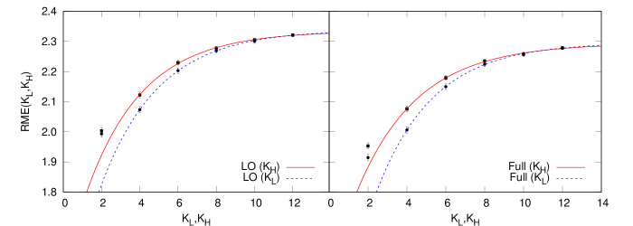
Figure 1: RME values computed as function of the maximum $K$ used in the expansion of the ${}^{6}{\rm Li}$ ($K_{L}$, circles) and ${}^{6}{\rm He}$ ($K_{H}$, squares) wave functions for the SRG2.0 version of the E interaction. The left (right) panel corresponds to results obtained with the LO (up to N3LO) axial current. The solid red (dashed blue) line is a fit to the calculated RMEs as function of $K_{L}$ ($K_{H}$); see text for further explanations. All remaining interactions exhibit a similar pattern of convergence.

E-model
	LO	N2LO(RC)	N3LO(OPE)	N3LO(CT)	N3LO(CT)/$z^{\rm E}_{0}$ [fm-3]	Full
SRG1.2	2.345(2)	$-$0.019	$-$0.038(1)	$-$0.018	$-$0.162(1)	2.271(3)
SRG1.5	2.342(3)	$-$0.021	$-$0.029(1)	$-$0.011	$-$0.185(1)	2.281(2)
SRG1.8	2.327(3)	$-$0.022	$-$0.019(1)	$-$0.008	$-$0.198(1)	2.281(4)
SRG2.0	2.338(3)	$-$0.022	$-$0.013(1)	$-$0.008	$-$0.202(1)	2.297(2)
bare	2.321(9)	$-$0.023	0.002(1)	$-$0.004	$-$0.211(1)	2.303(11)
P-model
	LO	N2LO(RC+$\Delta$)	N3LO(OPE)	N3LO(CT)	N3LO(CT)/$z^{\rm P}_{0}$ [fm-3]	Full
SRG1.2	2.354(1)	$-$0.033(1)	0.011	$-$0.066	$-$0.143(1)	2.265(2)
SRG1.5	2.331(4)	$-$0.030(1)	0.016	$-$0.066	$-$0.166(1)	2.251(3)
SRG1.8	2.329(5)	$-$0.023(1)	0.020	$-$0.068	$-$0.177(1)	2.257(4)
SRG2.0	2.322(6)	$-$0.019(1)	0.022	$-$0.070	$-$0.185(1)	2.260(11)
NV2-Ia + 3b(VMC) King et al. (2020)	2.200	0.022	0.039	$-$0.005	$-$0.009	2.256
NV2-Ia + 3b(GFMC) King et al. (2020)	2.130					2.201
Exp. Knecht et al. (2012)						2.1609(40)

Table 4: Extrapolated RMEs in ${}^{6}{\rm He}$ $\beta$-decay. The results are obtained by using SRG-evolved versions of the E and P models with $\Lambda_{\text{SRG}}=1.2,1.5,1.8,2.0$ fm^-1; $3N$ interactions are not included. Columns labeled LO, N2LO(RC), N3LO(OPE), and N3LO(CT) refer to the contributions given by the axial currents of Eqs. (1), (2), (• ‣ II), and (5), respectively; the column labeled N2LO(RC+$\Delta$) refers to the cumulative contribution of the axial currents of Eqs. (2) and (3). Note that the N3LO(CT) results have been divided out by the $z_{0}$ values listed in Table 2. The errors, when shown, are associated with the extrapolation; when they are not explicitly indicated, they are below the precision reported in the table. For a qualitative comparison, we also list the results of Ref. King et al. (2020) obtained with the P model (including $3N$ interactions), and the experimental value from Ref. Knecht et al. (2012).

Considering separately the contributions beyond LO, we observe that they do not present any particular convergence pattern. However, the calculations for $8\leq K_{L},K_{H}\leq 12$ are compatible within twice the statistical error bars of the Monte Carlo integration. Therefore, we consider as our best estimate the weighted average between the values obtained in the range $8\leq K_{L},K_{H}\leq 12$. We note that the convergence pattern of these contributions is independent of the interaction model (either E or P) and the value of $\Lambda_{\text{SRG}}$. The extrapolated values of the RME for each individual component of the current as well as for the full current are reported in Table 4. We find that two-body currents give a overall correction of opposite sign to the LO contribution, of the order of $\sim 3/4\%$, in line with the results of Refs. Vaintraub et al. (2009); Gysbers et al. (2019). However, a closer inspection of the table suggests a more complex situation.

From the first column of Table 4, the LO contribution seems to have a weak dependence on $\Lambda_{\text{SRG}}$: the larger is $\Lambda_{\text{SRG}}$, the smaller is the resulting LO contribution. This same sensitivity is also shown in Fig. 8 of Ref. Gysbers et al. (2019) and, as demonstrated by the authors of that paper, it is removed by including the SRG-induced two-body operators corresponding to the LO current. By comparing the results for the bare E model with its SRG evolved versions, the difference is of the order of $\sim 0.5\%$ and we would have expected a similar difference also in the case of the P model, had we been able to use the bare interaction. However, the results reported in Ref. King et al. (2020) show that at least a correction of the order of $5\%$ is needed. This extra quenching of the LO contribution comes from $3N$ interaction effects Wiringa et al. .

The N2LO(RC) contribution, which only consists of relativistic corrections to the LO Gamow-Teller operator, appears to be independent of the SRG-evolution parameter for both the E and P models. By contrast, the N2LO($\Delta$) contribution strongly depends on $\Lambda_{\text{SRG}}$, and is responsible for generating the pattern shown in Table 4. It starts off negative for $\Lambda_{\rm SRG}\,$=$\,1.2$ fm^-1, increases monotonically, and becomes positive for $\Lambda_{\rm{SRG}}\,$=$\,2.0$ fm^-1. In Ref. King et al. (2020) (with the bare P interaction) this contribution is found to be positive and larger than the negative N2LO(RC) contribution, resulting in an overall positive value for the sum. Here, the situation is reversed, and even at $\Lambda_{\rm SRG}\,$=$\,2.0$ fm^-1 the sum of the N2LO(RC) and N2LO($\Delta$) contributions remains negative. Such a difference is clearly due to SRG-evolution effects.

The N3LO(OPE) contribution also depends strongly on $\Lambda_{\text{SRG}}$, see Table 4. For the E model, it starts off negative at low $\Lambda_{\text{SRG}}$, and increases monotonically as $\Lambda_{\text{SRG}}$ increases, becoming positive in the limit $\Lambda_{\text{SRG}}\longrightarrow\infty$, corresponding to the bare interaction. This is a clear indication that a proper SRG evolution of the N3LO(OPE) current—as well as the N2LO($\Delta$) current, discussed above—is needed to obtain reliable estimates. Such a program has been partially carried out in Ref. Gysbers et al. (2019). However, to best of our knowledge, three body induced axial currents generated by the SRG evolution have not been included. The results obtained with the P model show the same behavior as function of $\Lambda_{\text{SRG}}$. However, in this case the N3LO(OPE) contribution is positive for all $\Lambda_{\rm SRG}$ used, and the calculations seem to go in the direction of Ref. King et al. (2020) when $\Lambda_{\text{SRG}}$ increases. However, we should point out that, because of cancellations between the terms proportional to $c_{3}$ and $c_{4}$, the overall N3LO(OPE) contribution is rather sensitive to the actual values of these LECs, in particular their ratio $c_{3}/c_{4}$. Lastly, for this contribution we do not expect significant effects from $3N$ interactions, since the latter do not affect appreciably the short-range behavior of two-nucleon densities. These densities, and the resulting change of sign between the E and P N3LO(OPE) contributions, are studied in the next section.

The N3LO(CT) contributions are found to be negative for both interaction models. When divided out by the LEC $z_{0}$—column labeled N3LO(CT)/$z_{0}$—they are almost identical between the E and P models. The results reported in Table 4 exhibit a significant dependence on the SRG-evolution parameter. It is interesting to note, however, how these results, when they are multiplied by the fitted values of $z_{0}$ from Table 2, become essentially independent of $\Lambda_{\text{SRG}}$ for the P model. By contrast, in the case of the E model the results remain $\Lambda_{\text{SRG}}$-dependent, albeit the trend is inverted (rather than decreasing, they increase as $\Lambda_{\rm SRG}$ increases). It seems that $z_{0}$ can absorb, at least partially, the effect of the SRG evolution of the currents. By comparing our results for the P model with those of Ref. King et al. (2020), there is almost one order of magnitude of difference.

IV.1 Two-body transition densities

In order to understand the differences between the results obtained with the two different chiral interactions, we compute the two-body transition density, which we define as King et al. (2020); Schiavilla et al. (1998)

$$\text{RME(2b)}=4\pi\int_{0}^{\infty}\,dr\,r^{2}\,\rho^{2b}(r)\,,$$ (34)

where $r$ is the distance between two nucleons and 2b stands for N2LO($\Delta$) (only for the P model), N3LO(OPE), and N3LO(CT). In Fig. 2 we report the two-body densities computed using $\Lambda_{\text{SRG}}=2.0$ fm^-1 for the E and P models. Their shape is independent on the $\Lambda_{\text{SRG}}$ value, except for the N2LO($\Delta$) contribution for the P-model where for $\Lambda_{\text{SRG}}=1.2,1.5,1.8$ fm^-1 the two-body transition densities result of opposite sign.

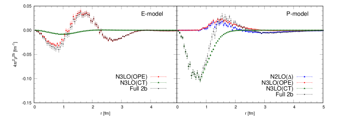
Figure 2: Two-body densities defined in Eq. (34) for the SRG-evolved versions of the E and P interactions corresponding to $\Lambda_{\text{SRG}}=2.0$ fm^-1. Similar results are obtained for all other $\Lambda_{\text{SRG}}$ considered in this work, except for the N2LO($\Delta$) contribution for the P-model where for $\Lambda_{\text{SRG}}=1.2,1.5,1.8$ fm^-1 the two-body transition densities result of opposite sign.

Inspection of the two panels in Fig. 2 indicates that the N3LO(OPE) densities corresponding to the E and P models are rather different. As a matter of fact, the shape of these densities is determined by the cancellation between the two components of the current proportional to the LECs $c_{3}$ and $c_{4}$ through $\alpha_{1}$ and $\alpha_{2}$ in Eq. (• ‣ II). In Fig. 3 we plot the separated contributions for the two interactions. In the E model there is a double lobe structure for both the $c_{3}$ and $c_{4}$ components. This, and the fact that the maxima of the second lobes do not coincide, generate a three-lobe structure with two of the lobes negative and one positive. In the P model, the $c_{3}$ and $c_{4}$ components have both just one lobe, which generates a single lobe in the total contribution (see Fig. 3). This is qualitatively consistent with the results reported in Ref. King et al. (2020).

The difference in the N3LO(OPE) densities of the E and P models originates from that in the corresponding correlation functions entering the current, see Eqs. (6)–(7) and Eqs. (11)–(12). We plot those proportional to $c_{3}$ (with $c_{3}\,$=$\,1$ in units of GeV^-1 to make the comparison meaningful) in Fig. 4. In the region $r\lesssim 3$ fm, their shapes are affected by the choice of regulator. This also produces the sign inversion between the E- and P-model $c_{3}$ (and $c_{4}$) contributions, shown in Fig. 3.

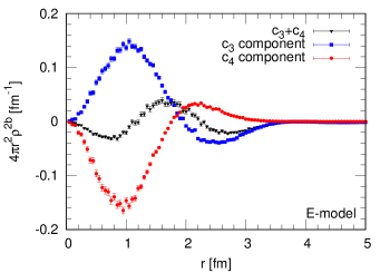
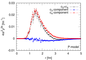
Figure 3: Two-body densities for the N3LO(OPE) contribution (solid points) computed with the SRG-evolved versions of the E and P interactions with $\Lambda_{\text{SRG}}\,$=$\,2.0$ fm^-1. The blue (red) points indicate the density corresponding to the component proportional to $c_{3}$ ($c_{4}$) only.

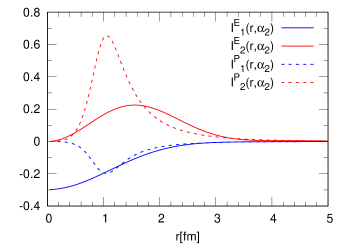
Figure 4: Correlation functions in the N3LO(OPE) current for the E model from Eqs. (6)–(7) (full lines), and the P model from Eqs. (11)–(12) (dashed lines). In the figure we show the $I_{1}$ and $I_{2}$ functions proportional to $c_{3}$ only, but with $c_{3}\,$ set to 1 in units of GeV^-1.

For the N3LO(CT) contribution, the main difference between the two interactions is the presence of a second tiny lobe at $r\approx 2$ fm in the E model, and the fact that the maximum is shifted towards larger $r$-values (around 1 fm) compared to that in the P model. Also in this case, the origin of the differences among the two-body densities comes from the different behavior of the correlation functions given in Eqs. (9) and  (14). The results obtained with the P model with $\Lambda_{\text{S}RG}=2.0$ for the N2LO($\Delta$), N3LO(OPE), and N3LO(CT) densities are in qualitative agreement with those of Ref. King et al. (2020).

V Conclusions

In this work, we have reported on a study of the ${}^{6}{\rm He}$ GTME, using different chiral two-nucleon interactions, the N2LO450 Entem et al. (2017) and NV2-Ia Piarulli et al. (2016) models. Both models have been evolved via SRG unitary transformations corresponding to parameters $\Lambda_{\rm SRG}$ between 1.2 and 2.0 fm^-1. We have neglected $3N$ and SRG-induced many-nucleon interaction effects, as well as SRG-induced many-body terms in the nuclear axial current.

The results are summarized in Table 4. We find for both models that all axial-current terms beyond LO yield a cumulative contribution, which (in magnitude) amounts to a 3% correction of the LO Gamow-Teller contribution. We also find this cumulative contribution to have the opposite sign of the LO one, in agreement with the results of Refs. Gysbers et al. (2019); Vaintraub et al. (2009). The contributions of two-body currents, in particular of N3LO(OPE), while small, depend strongly on the parameter $\Lambda_{\rm SRG}$, suggesting that a consistent evolution of these currents (together with the one-body current) may be necessary in order to obtain reliable predictions. The same conclusion can also be drawn by considering the results for the tritium $\beta$-decay in Table 2.

We have been unable to reproduce the sign of the beyond-LO contributions obtained in Ref. King et al. (2020) with the bare NV2-Ia interaction. This can be traced back to differences in the contributions associated with the N2LO(RC) and N3LO(CT) currents. The origin of these differences is unclear. We conjecture they might be due to the absence, in the present HH calculation, of the multi-nucleon terms induced by the SRG transformation in the interactions and currents. By contrast, there is qualitative agreement in the shape of the two-body transition densities calculated here and in Ref. King et al. (2020).

We have shown that the N3LO(OPE) contribution is opposite in sign for the SRG-evolved N2LO450 and NV2-Ia interactions. The corresponding transition densities in Fig. 2 have different shapes, reflecting the different behavior of the correlation functions entering the N3LO(OPE) current, see Fig. 4. This behavior follows in turn from the different choice of short-range regulators we have adopted in the N2LO450 and NV2-Ia calculations. We note in closing that the sign difference in the N3LO(OPE) contribution obtained in Refs. Gysbers et al. (2019) and King et al. (2020) may have a similar origin.

Appendix A Classes of convergence

In this Appendix we define the classes of convergence in which we separate the HH states. This definition is based on a couple of criteria. The first one is that, as the value $\ell_{\text{sum}}=\ell_{1}+\ell_{2}+\ell_{3}+\ell_{4}+\ell_{5}$ increases, so does the centrifugal barrier, which keeps nucleons apart from each other, thus reducing the effect of correlations induced by the nuclear interactions. The second criterion accounts for the fact that the $2N$ interaction favors two-body correlations and so the HH states with non-zero quantum numbers for the couple $(i,j)$ are privileged. These states can be easily selected by imposing $\ell_{i}=0$ with $i=1,2,3,4$. Furthermore, the HH states can also be classified on the basis of their $LST$ quantum numbers (or partial waves). Indeed, in the ${}^{6}{\rm Li}$ and ${}^{6}{\rm He}$ nuclei the most important partial waves are the $S$ and $D$ waves, while all the others give small contribution to the binding energy.

class	partial waves	$\ell_{\text{sum}}$	$K_{iM}$
$C_{1}^{L}$	${}^{3}S_{1}$	$\ell_{\text{sum}}=0$	14
$C_{2}^{L}$	${}^{3}D_{1}$,${}^{5}D_{1}$,${}^{7}D_{1}$	$\ell_{5}=2$, $\sum_{i=1,4}\ell_{i}=0$	12
$C_{3}^{L}$	${}^{3}S_{1}$	$\ell_{\text{sum}}=2$	10
$C_{4}^{L}$	${}^{3}D_{1}$,${}^{5}D_{1}$,${}^{7}D_{1}$	$\ell_{\text{sum}}=2$, not included in $C_{2}^{L}$	10
$C_{5}^{L}$	${}^{1}P_{1}$,${}^{3}P_{1}$,${}^{5}P_{1}$	$\ell_{\text{sum}}=2$	8
$C_{6}^{L}$	${}^{5}F_{1}$,${}^{7}F_{1}$,${}^{7}G_{1}$	$\ell_{\text{sum}}=4$	8

Table 5: Definition of the classes of hyperangular-spin-isospin states $\Psi^{KLSTJ\pi}_{\alpha}$ [see Eq. (27)] used for the ${}^{6}{\rm Li}$ bound state as given in Ref. Gnech et al. (2020). The classes are defined by selecting particular values of the total orbital angular momentum $L$ and total spin $S$ (indicated by the spectroscopic notation ${}^{2S+1}L_{J}$), and the value of $\ell_{\text{sum}}=\ell_{1}+\cdots+\ell_{5}$, given in the second and third column, respectively. In the last column, the maximum $K$ value adopted in the expansion is reported for each class.

In Tables 5 and 6 we report the properties of the HH states used to define a given class for, respectively, ${}^{6}{\rm Li}$ and ${}^{6}{\rm He}$. For each class $i$ we also give the maximum value of $K$ we have adopted ($K_{iM}$). A more detailed discussion of the class definition for ${}^{6}{\rm Li}$ can be found in Ref. Gnech et al. (2020). Here, we only note that in the case of ${}^{6}{\rm He}$ we divide the HH states in six different classes. Classes $C_{1}^{H}$ and $C_{2}^{H}$ are the main components of the ${}^{6}{\rm He}$ ground state, since they correspond to two-body correlated states having $L\,$=$\,0$ and 2, respectively. For both of them we reach $K$ values up to $K_{1M}\,$=$\,K_{2M}\,$=$\,12$. Classes $C_{3}^{H}$ and $C_{4}^{H}$ contain HH states that generate many-body correlations for the $S$ and $D$ wave, respectively. For this reason, their contribution to the binding energy is smaller and we stop at $K_{3M}\,$=$\,K_{4M}\,$=$\,10$. Class $C_{5}^{H}$ contains HH states with $L\,$=$\,1$, which are less important in the construction of the wave function. We therefore keep $K$ values up to $K_{5M}=8$ for these. Finally, class $C_{6}^{H}$ consists of HH states with $L\,$=$\,3$. Their contribution to the binding energy is tiny and so we select $K_{6M}\,$=$\,8$.

class	partial waves	$\ell_{\text{sum}}$	$K_{iM}$
$C_{1}^{H}$	${}^{1}S_{0}$	$\ell_{\text{sum}}=0$	12
$C_{2}^{H}$	${}^{5}D_{0}$	$\ell_{5}=2$,  $\sum_{i=1,4}\ell_{i}=0$	12
$C_{3}^{H}$	${}^{1}S_{0}$	$\ell_{\text{sum}}=2$	10
$C_{4}^{H}$	${}^{5}D_{0}$	$\ell_{\text{sum}}=2$,  not included in $C_{2}^{H}$	10
$C_{5}^{H}$	${}^{3}P_{0}$	$\ell_{\text{sum}}=2$	8
$C_{6}^{H}$	${}^{7}F_{0}$	$\ell_{\text{sum}}=4$	8

Table 6: Same as Table 5 but for ${}^{6}{\rm He}$.

Appendix B Convergence of the HH expansion

In this appendix we study the convergence of the ${}^{6}{\rm Li}$ and ${}^{6}{\rm He}$ binding energies and discuss the extrapolation method. The convergence is studied class by class. When studying the convergence of a generic class $C_{i}$, we include in the expansion all the HH states with $K\leq K_{i}$ and then vary $K_{i}$ between a minimum value and $K_{iM}$. For the other classes $C_{j}$ with $j\neq i$, we include all HH states up to $K_{jM}$. Note that for classes $C_{1}^{L}$ and $C_{2}^{L}$ ($C_{1}^{H}$ and $C_{2}^{H}$) in ${}^{6}{\rm Li}$ (${}^{6}{\rm He}$), because of the procedure used for the selection of the linearly independent HH states, we cannot include, respectively, classes $C_{3}^{L}$ and $C_{4}^{L}$ ($C_{3}^{H}$ and $C_{4}^{H}$). The ${}^{6}{\rm Li}$ and ${}^{6}{\rm He}$ binding energies are listed in Tables 7 and 8.

						E-model					P-model
$K_{1}$	$K_{2}$	$K_{3}$	$K_{4}$	$K_{5}$	$K_{6}$	SRG$1.2$	SRG$1.5$	SRG$1.8$	SRG$2.0$	bare	SRG$1.2$	SRG$1.5$	SRG$1.8$	SRG$2.0$
2	12		10	8	8	27.000	26.782	25.537	24.621	19.844	27.088	27.022	25.976	25.169
4	12		10	8	8	30.573	30.892	29.909	29.066	24.238	30.766	31.259	30.404	29.566
6	12		10	8	8	31.645	32.468	31.845	31.152	26.619	31.857	32.872	32.365	31.632
8	12		10	8	8	31.949	32.991	32.559	31.957	27.732	32.163	33.400	33.072	32.387
10	12		10	8	8	32.057	33.185	32.822	32.254	28.279	32.271	33.594	33.331	32.662
12	12		10	8	8	32.095	33.257	32.923	32.368	28.554	32.308	33.669	33.435	32.776
14	12		10	8	8	32.108	33.284	32.960	32.410	28.725	32.322	33.696	33.474	32.819
14	2	10		8	8	30.917	30.480	27.946	25.917	16.222	31.195	31.076	28.586	26.078
14	4	10		8	8	31.555	31.643	29.593	27.800	18.602	31.808	32.191	30.199	27.957
14	6	10		8	8	31.951	32.712	31.591	30.403	23.451	32.176	33.174	32.120	30.600
14	8	10		8	8	32.038	33.038	32.373	31.542	26.315	32.256	33.469	32.881	31.832
14	10	10		8	8	32.060	33.138	32.650	31.974	27.624	32.276	33.558	33.160	32.329
14	12	10		8	8	32.068	33.177	32.765	32.160	28.265	32.283	33.593	33.277	32.554
14	12	6	10	8	8	32.109	33.287	32.964	32.416	28.734	32.323	33.698	33.476	32.823
14	12	8	10	8	8	32.142	33.333	33.016	32.469	28.779	32.355	33.744	33.528	32.873
14	12	10	10	8	8	32.158	33.358	33.047	32.501	28.813	32.371	33.769	33.558	32.904
14	12	10	4	8	8	32.074	33.187	32.779	32.175	28.285	32.290	33.604	33.293	32.572
14	12	10	6	8	8	32.124	33.276	32.904	32.319	28.480	32.338	33.691	33.418	32.720
14	12	10	8	8	8	32.150	33.336	33.003	32.442	28.683	32.364	33.748	33.516	32.843
14	12	10	10	8	8	32.158	33.358	33.047	32.501	28.813	32.371	33.769	33.558	32.904
14	12	10	10	2	8	32.078	33.181	32.769	32.163	28.228	32.303	33.611	33.292	32.567
14	12	10	10	4	8	32.132	33.287	32.917	32.332	28.462	32.348	33.703	33.418	32.727
14	12	10	10	6	8	32.151	33.335	33.000	32.437	28.656	32.364	33.748	33.512	32.837
14	12	10	10	8	8	32.158	33.358	33.047	32.501	28.813	32.371	33.769	33.558	32.904
14	12	10	10	8	4	32.145	33.314	32.953	32.371	28.530	32.359	33.730	33.470	32.773
14	12	10	10	8	6	32.154	33.342	33.007	32.442	28.662	32.367	33.755	33.521	32.844
14	12	10	10	8	8	32.158	33.358	33.047	32.501	28.813	32.371	33.769	33.558	32.904

Table 7: Convergence of the ${}^{6}{\rm Li}$ binding energy for the different classes $C_{1}^{L}$–$C_{6}^{L}$, into which the HH states have been divided. All results are in MeV units.

						E-model					P-model
$K_{1}$	$K_{2}$	$K_{3}$	$K_{4}$	$K_{5}$	$K_{6}$	SRG$1.2$	SRG$1.5$	SRG$1.8$	SRG$2.0$	bare	SRG$1.2$	SRG$1.5$	SRG$1.8$	SRG$2.0$
2	12		10	10	6	24.114	24.294	23.330	22.500	17.961	23.822	23.905	22.953	22.117
4	12		10	10	6	27.176	27.585	26.749	25.985	21.585	27.253	27.742	26.969	26.176
6	12		10	10	6	28.295	29.194	28.713	28.108	24.054	28.419	29.449	29.053	28.398
8	12		10	10	6	28.651	29.764	29.457	28.933	25.149	28.789	30.046	29.819	29.209
10	12		10	10	6	28.802	30.010	29.776	29.285	25.721	28.943	30.301	30.143	29.551
12	12		10	10	6	28.870	30.123	29.921	29.444	26.024	29.013	30.419	30.295	29.712
12	4	10		10	6	28.442	28.847	27.274	25.796	17.845	28.609	29.233	27.696	25.831
12	6	10		10	6	28.720	29.586	28.652	27.593	21.218	28.871	29.917	29.019	27.647
12	8	10		10	6	28.805	29.900	29.383	28.647	23.807	28.950	30.205	29.739	28.786
12	10	10		10	6	28.833	30.011	29.669	29.080	25.048	28.976	30.308	30.028	29.283
12	12	10		10	6	28.844	30.058	29.799	29.284	25.692	28.986	30.352	30.163	29.528
12	12	4	4	10	6	28.843	30.058	29.802	29.288	25.705	28.986	30.355	30.172	29.541
12	12	6	6	10	6	28.860	30.093	29.857	29.357	25.833	29.003	30.389	30.230	29.616
12	12	8	8	10	6	28.878	30.132	29.923	29.440	25.982	29.021	30.426	30.296	29.703
12	12	10	10	10	6	28.887	30.151	29.956	29.483	26.074	29.029	30.445	30.329	29.749
12	12	10	10	2	6	28.719	29.831	29.501	28.956	25.251	28.884	30.153	29.891	29.226
12	12	10	10	4	6	28.799	29.961	29.662	29.127	25.438	28.952	30.270	30.042	29.388
12	12	10	10	6	6	28.856	30.081	29.842	29.340	25.766	29.002	30.380	30.217	29.601
12	12	10	10	8	6	28.876	30.127	29.916	29.430	25.939	29.020	30.423	30.288	29.693
12	12	10	10	10	6	28.887	30.151	29.956	29.483	26.074	29.029	30.445	30.329	29.749
12	12	10	10	10	4	28.886	30.148	29.948	29.472	26.044	29.029	30.443	30.321	29.736
12	12	10	10	10	6	28.887	30.151	29.956	29.483	26.074	29.029	30.445	30.329	29.749

Table 8: Same as Table 7 but for ${}^{6}{\rm He}$.

We assume that for each class of convergence the behavior of the binding energy as function of $K$ is exponential, namely

$$B_{i}(K)=B_{i}(\infty)+a_{i}\,{\rm e}^{-b_{i}K}\,,$$ (35)

where $B_{i}(\infty)$ is the asymptotic binding energy of class $C_{i}$ as $K\longrightarrow\infty$. The parameters $a_{i}$ and $b_{i}$ depend on the interaction model and on the specific class of HH states we are studying. The values of $B_{i}(K)$ are those reported in Tables 7 and 8. By defining the function

$$\Delta_{i}(K)=B_{i}(K)-B_{i}(K-2)\,,$$ (36)

it is possible to compute, for each class, the “missing” binding energy due to the truncation of the expansion to a finite $K_{iM}$ as illustrated in Ref. Viviani et al. (2005), namely,

$$\left(\Delta B\right)_{i}=\sum_{K=K_{iM}+2,K_{iM}+4,\dots}\Delta_{i}(K)\,.$$ (37)

By using Eq. (35), we obtain

$$\left(\Delta B\right)_{i}=\Delta_{i}(K_{iM})\frac{1}{{\rm e}^{2b_{i}}-1}\,.$$ (38)

The “total missing” binding energy is then computed as

$$\left(\Delta B\right)_{T}=\sum_{i=1,6}\Delta_{i}(K_{iM})\frac{1}{{\rm e}^{2b_{i}}-1}\,.$$ (39)

In order to determine the coefficients $b_{i}$ for each class, we proceed as follows. For classes $C_{1}^{L}$, $C_{2}^{L}$, and $C_{1}^{H}$, we estimate the $b_{i}$ by performing a fit to the binding energy values of Tables 7 and 8, using Eq. (35). We propagate the error on the resulting $b_{i}$ to compute the error on $\left(\Delta B\right)_{i}$. For classes $C_{5}^{L}$, $C_{2}^{H}$, and $C_{5}^{H}$, the quality of the fit is not good enough to obtain a sensible estimate. In these cases, we consider a reasonable range for $b_{i}$,

$$\min{\{b_{i}^{0},b_{i}^{1}\}}\leq b_{i}\leq\max{\{b_{i}^{0},b_{i}^{1}\}}\ ,$$ (40)

where $b_{i}^{0}$ and $b_{i}^{1}$ are computed from

$$\frac{\Delta_{i}(K_{iM}-2)}{\Delta_{i}(K_{iM})}={\rm e}^{2b_{i}^{0}}\,,\qquad\frac{\Delta_{i}(K_{iM}-4)}{\Delta_{i}(K_{iM}-2)}={\rm e}^{2b_{i}^{1}}\ .$$ (41)

We use the central value of the interval as the best estimate, and the range as error bar. For classes $C_{3}^{L}$, $C_{4}^{L}$, and $C_{3}^{H}+C_{4}^{H}$, we simply estimate $b_{i}$ from

$$\frac{\Delta_{i}(K_{iM}-2)}{\Delta_{i}(K_{iM})}={\rm e}^{2b_{i}}\,.$$ (42)

In such cases, we use these $b_{i}$ to obtain the missing energy, and estimate the error as half of this missing energy. Finally, for classes $C_{6}^{L}$ and $C_{6}^{H}$ it is not possible to obtain reliable values for the $b_{i}$. Therefore, we estimate the missing binding energy as $\Delta_{i}(K_{iM})$ and the error as half of it. In Tables 9 and 10 we report the missing binding energy with the associated error for each of the six classes we have considered.

	E-model					P-model
	SRG$1.2$	SRG$1.5$	SRG$1.8$	SRG$2.0$	bare	SRG$1.2$	SRG$1.5$	SRG$1.8$	SRG$2.0$
$C_{1}^{L}$	0.007(0)	0.016(0)	0.022(0)	0.025(0)	0.175(0)	0.008(0)	0.016(0)	0.023(1)	0.026(1)
$C_{2}^{L}$	0.003(0)	0.018(2)	0.066(5)	0.118(7)	0.557(19)	0.002(0)	0.016(2)	0.071(4)	0.173(10)
$C_{3}^{L}$	0.015(8)	0.030(15)	0.046(23)	0.049(24)	0.105(53)	0.016(8)	0.030(15)	0.041(20)	0.051(25)
$C_{4}^{L}$	0.004(2)	0.013(6)	0.035(18)	0.054(27)	0.231(116)	0.003(1)	0.012(6)	0.032(16)	0.060(30)
$C_{5}^{L}$	0.004(0)	0.020(1)	0.061(1)	0.102(3)	0.319(25)	0.005(1)	0.019(1)	0.074(60)	0.123(24)
$C_{6}^{L}$	0.008(4)	0.032(16)	0.080(40)	0.118(59)	0.302(151)	0.008(4)	0.030(15)	0.074(37)	0.120(60)
Tot.	0.033(9)	0.113(23)	0.288(50)	0.442(70)	1.515(200)	0.034(9)	0.107(22)	0.292(75)	0.527(76)

Table 9: Missing binding energies corresponding to the E and P interaction models, obtained for each of the six classes of convergence we have considered for ${}^{6}{\rm Li}$. In parentheses, we report the errors on the extrapolation; note that $(0)$ indicates that the error does not affect the last digit reported in the result.

	E-model					P-model
	SRG$1.2$	SRG$1.5$	SRG$1.8$	SRG$2.0$	bare SRG$1.2$	SRG$1.5$	SRG$1.8$	SRG$2.0$
$C_{1}^{H}$	0.051(1)	0.088(3)	0.111(3)	0.121(3)	0.333(4)	0.052(2)	0.091(4)	0.116(6)	0.123(7)
$C_{2}^{H}$	0.006(1)	0.030(5)	0.095(13)	0.161(21)	0.643(52)	0.006(1)	0.028(4)	0.104(15)	0.213(26)
$C_{3}^{H}$	0.009(4)	0.018(9)	0.033(16)	0.046(23)	0.148(74)	0.006(3)	0.020(10)	0.033(17)	0.052(26)
$C_{4}^{H}$
$C_{5}^{H}$	0.009(4)	0.020(6)	0.036(11)	0.054(22)	0.251(213)	0.007(2)	0.018(5)	0.040(16)	0.061(26)
$C_{6}^{H}$	0.002(1)	0.006(3)	0.016(8)	0.022(11)	0.060(30)	0.002(1)	0.004(2)	0.016(8)	0.026(13)
Tot.	0.078(7)	0.162(13)	0.292(25)	0.405(40)	1.434(233)	0.072(5)	0.161(13)	0.309(29)	0.474(47)

Table 10: Same as Table 9 but for ${}^{6}{\rm He}$.

References

- Chou et al. (1993) W.-T. Chou, E. K. Warburton, and B. A. Brown, Phys. Rev. C 47, 163 (1993).
- Engel and Menéndez (2017) J. Engel and J. Menéndez, Reports on Progress in Physics 80, 046301 (2017).
- Pastore et al. (2018) S. Pastore, A. Baroni, J. Carlson, S. Gandolfi, S. C. Pieper, R. Schiavilla, and R. B. Wiringa, Phys. Rev. C 97, 022501 (2018).
- Gysbers et al. (2019) P. Gysbers, G. Hagen, J. Holt, and et al., Nat. Phys. 15, 428 (2019).
- King et al. (2020) G. B. King, L. Andreoli, S. Pastore, M. Piarulli, R. Schiavilla, R. B. Wiringa, J. Carlson, and S. Gandolfi, Phys. Rev. C 102, 025501 (2020).
- Kievsky et al. (2008) A. Kievsky, S. Rosati, M. Viviani, L. Marcucci, and L. Girlanda, J. Phys. G: Nucl. Part. Phys. 35, 063101 (2008).
- Marcucci et al. (2020) L. E. Marcucci, J. Dohet-Eraly, L. Girlanda, A. Gnech, A. Kievsky, and M. Viviani, Front. Phys. 8, 69 (2020).
- Gnech et al. (2020) A. Gnech, M. Viviani, and L. E. Marcucci, Phys. Rev. C 102, 014001 (2020).
- Schiavilla et al. (2021) R. Schiavilla, L. Girlanda, A. Gnech, A. Kievsky, A. Lovato, L. E. Marcucci, M. Piarulli, and M. Viviani, Phys. Rev. C 103, 054003 (2021).
- Entem et al. (2017) D. R. Entem, R. Machleidt, and Y. Nosyk, Phys. Rev. C 96, 024004 (2017).
- Piarulli et al. (2015) M. Piarulli, L. Girlanda, R. Schiavilla, R. N. Pérez, J. E. Amaro, and E. R. Arriola, Phys. Rev. C 91, 024003 (2015).
- Piarulli et al. (2016) M. Piarulli, L. Girlanda, R. Schiavilla, A. Kievsky, A. Lovato, L. E. Marcucci, S. C. Pieper, M. Viviani, and R. B. Wiringa, Phys. Rev. C 94, 054007 (2016).
- Bogner et al. (2007) S. Bogner, R. Furnstahl, and R. Perry, Phys. Rev. C 75, 061001 (2007).
- Baroni et al. (2016) A. Baroni, L. Girlanda, A. Kievsky, L. E. Marcucci, R. Schiavilla, and M. Viviani, Phys. Rev. C 94, 024003 (2016).
- Baroni et al. (2018) A. Baroni, R. Schiavilla, L. E. Marcucci, L. Girlanda, A. Kievsky, A. Lovato, S. Pastore, M. Piarulli, S. C. Pieper, M. Viviani, and R. B. Wiringa, Phys. Rev. C 98, 044003 (2018).
- Zernike and Brinkman (1935) F. Zernike and H. Brinkman, Proc. Kon. Ned. Acad. Wensch. 33, 3 (1935).
- de la Ripelle (1983) M. F. de la Ripelle, Ann. Phys. 147, 281 (1983).
- Abramowitz and Stegun (1970) M. Abramowitz and I. Stegun, Handbook of Mathematical Functions (Dover Publications, Inc., New York, 1970).
- Cullum and Willoughby (1981) J. Cullum and R. Willoughby, J. Comp. Phys. 44, 329 (1981).
- Tilley et al. (2002) D. Tilley, C. Cheves, J. Godwin, G. Hale, H. Hofmann, J. Kelley, C. Sheu, and H. Weller, Nuclear Physics A 708, 3 (2002).
- Knecht et al. (2012) A. Knecht, R. Hong, D. W. Zumwalt, B. G. Delbridge, A. García, P. Müller, H. E. Swanson, I. S. Towner, S. Utsuno, W. Williams, and C. Wrede, Phys. Rev. C 86, 035506 (2012).
- Vaintraub et al. (2009) S. Vaintraub, N. Barnea, and D. Gazit, Phys. Rev. C 79, 065501 (2009).
- (23) R. B. Wiringa, G. B. King, and S. Pastore, private communication.
- Schiavilla et al. (1998) R. Schiavilla, V. G. J. Stoks, W. Glöckle, H. Kamada, A. Nogga, J. Carlson, R. Machleidt, V. R. Pandharipande, R. B. Wiringa, A. Kievsky, S. Rosati, and M. Viviani, Phys. Rev. C 58, 1263 (1998).
- Viviani et al. (2005) M. Viviani, A. Kievsky, and S. Rosati, Phys. Rev. C 71, 024006 (2005).