ALMA Observations of the Sub-kpc Structure of the Host Galaxy of a $z=6.5$ Lensed Quasar: A Rotationally-Supported Hyper-Starburst System at the Epoch of Reionization

Abstract

We report ALMA observations of the dust continuum and [C ii] emission of the host galaxy of J0439+1634, a gravitationally lensed quasar at $z=6.5$. Gravitational lensing boosts the source-plane resolution to $\sim 0\farcs 15$ $(\sim 0.8\text{ kpc})$. The lensing model derived from the ALMA data is consistent with the fiducial model in Fan et al. (2019) based on HST imaging. The host galaxy of J0439+1634 can be well-fitted by a Sérsic profile consistent with an exponential disk, both in the far-infrared (FIR) continuum and the [C ii] emission. The overall magnification is $4.53\pm 0.05$ for the continuum and $3.44\pm 0.05$ for the [C ii] line. The host galaxy of J0439+1634 is a compact ultra-luminous infrared galaxy, with a total star formation rate (SFR) of $1.56\times 10^{3}M_{\odot}/\text{year}$ after correcting for lensing and an effective radius of $0.74$ kpc. The resolved regions in J0439+1634 follow the “[C ii] deficit,” where the [C ii]-to-FIR ratio decreases with FIR surface brightness. The reconstructed velocity field of J0439+1634 appears to be rotation-like. The maximum line-of-sight rotation velocity of 130 km/s at a radius of 2 kpc. However, our data cannot be fit by an axisymmetric thin rotating disk, and the inclination of the rotation axis, $i$, remains unconstrained. We estimate the dynamical mass of the host galaxy to be $7.9\sin^{-2}(i)\times 10^{9}M_{\odot}$. J0439+1634 is likely to have a high gas-mass fraction and an oversized SMBH compared to local relations. The SFR of J0439+1634 reaches the maximum possible values, and the SFR surface density is close to the highest value seen in any star-forming galaxy currently known in the universe.

1 Introduction

In the past two decades, more than 200 quasars at $z>6$ have been discovered (e.g., Matsuoka et al., 2016, 2018a, 2018b, 2019; Venemans et al., 2013, 2015; Yang et al., 2019a, 2020; Wang et al., 2017, 2019b; Jiang et al., 2016; Bañados et al., 2016, 2018). Studies of the quasar host galaxies provide crucial knowledge about the co-evolution of supermassive black holes (SMBHs) with their host galaxies and environment in the early universe. Detecting the host galaxies of high-redshift quasars is challenging at rest-frame ultraviolet to near-infrared wavelengths, where the emission from the central quasar overwhelms the host galaxy (e.g., Mechtley et al., 2012; Marshall et al., 2020). As such, information about quasar host galaxies is mostly from the far-infrared (FIR) and sub-millimeter (sub-mm) regime (e.g., Riechers et al., 2009; Wang et al., 2008, 2010; Venemans et al., 2012). The dust continuum and atomic and molecular emission lines (for example, the [C ii] fine structure line and CO rotational lines) contain a wealth of information about the interstellar medium (ISM), including the dust mass and temperature (e.g., Beelen et al., 2006; Schreiber et al., 2018), the atomic and molecular gas mass (e.g., Weiß et al., 2005; Bolatto et al., 2013), and the gas-phase metallicity (e.g., Rigopoulou et al., 2018). Spatially resolved line emission also directly probes the gas-phase kinematics of quasar host galaxies and provides the only current way to measure their dynamical masses (e.g., Walter et al., 2009). The total-infrared (TIR) luminosity is widely used to estimate the star formation rate (SFR) (e.g., Murphy et al., 2011), assuming that the cool dust in the quasar host is dominantly heated by star formation (e.g., Beelen et al., 2006; Leipski et al., 2014).

With unprecedented sensitivity and resolving power, the Atacama Large Millimeter/Submillimeter Array (ALMA) has greatly improved our understanding of high-redshift quasars. To date, several tens of quasars at $z>6$ have been observed by ALMA, including about 15 at $z>6.5$. These observations led to an overall picture of the high-redshift quasar population: most of the high-redshift quasars are hosted by infrared-luminous, gas rich galaxies (e.g., Decarli et al., 2018; Venemans et al., 2018; Wang et al., 2019a; Shao et al., 2019), indicating active star formation $(\text{SFR}\gtrsim 10^{2}M_{\odot}\text{ yr}^{-1})$. The kinematics of the bright [C ii] emission line constrains the dynamical masses of quasar host galaxies. Compared to the local $M_{\text{BH}}-M_{\text{host}}$ relation (e.g., Kormendy & Ho, 2013), SMBHs in quasars at $z\gtrsim 6$ are oversized (e.g., Venemans et al., 2016; Decarli et al., 2018; Wang et al., 2019c). While SMBHs might grow earlier than their hosts at high redshift, this difference may be a result of selection effects, i.e., current quasar surveys are biased toward luminous quasars, which have massive SMBHs (e.g., Willott et al., 2015; Izumi et al., 2019).

At $z>6$, quasar host galaxies usually have sizes of $\sim 2-4\text{ kpc}$ (e.g., Decarli et al., 2018), although they can be as compact as $\sim 1\text{ kpc}$ (e.g., Venemans et al., 2017). Most ALMA observations of high-redshift quasars use beam sizes of $\gtrsim 0\farcs 3$, which marginally resolve these quasar host galaxies. These hosts have a variety of morphologies, ranging from a regular Gaussian profile (e.g., Shao et al., 2017; Venemans et al., 2018) to highly irregular, indicating an on-going merging system (e.g., Bañados et al., 2019; Neeleman et al., 2019). In a recent study, Venemans et al. (2019) reported 400-pc resolution imaging of a quasar host galaxy at redshift 6.6, which shows complex structures of dust continuum and [C ii] emission, including cavities with sizes of $\sim 0.5\text{ kpc}$. The authors propose that these cavities might be relevant to the energy output of the central active galactic nucleus (AGN). Sub-kpc resolution is thus necessary to the investigation of the structures in high-redshift quasars and to the understanding of SMBH-host coevolution.

Gravitational lensing acts as a natural telescope, significantly enhancing the angular resolution and the sensitivity of observations (e.g., Hezaveh et al., 2016; Litke et al., 2019; Inoue et al., 2020; Cheng et al., 2020; Spilker et al., 2020). In Fan et al. (2019), we reported the discovery of a gravitationally lensed quasar at $z=6.51$, J043947.08+163415.7 (hereafter J0439+1634). High-resolution images taken by Hubble Space Telescope (HST) reveal the multiple images of the quasar generated by gravitational lensing. The lensing model based on HST data suggests that J0439+1634 is a naked-cusp lens with three images, with a total magnification of $51.3\pm 1.4$. J0439+1634 is the only known lensed quasar at $z>5$ to date and provides an excellent chance to study a high-redshift quasar in enhanced spatial resolution due to its large lensing magnification.

Here we report the sub-mm continuum and [C ii] $158~{}\mu\text{m}$ emission line of J0439+1634 observed by ALMA at a resolution of $\sim 0\farcs 3$. With the help of lensing, we reach a physical resolution of $\sim 0.8\text{ kpc}$. We describe our data in Section 2. In Section 3, we describe the measurement of the dust continuum and [C ii] emission line, including the lens modeling and the reconstruction of the velocity field. We present the physical properties of J0439+1634 in Section 4 and discuss their implications for the evolutionary state of the quasar host galaxy in Section 5. We summarize this paper in Section 6. Throughout this paper, we use a $\Lambda$CDM universe with $H_{0}=70\text{ km s}^{-1}\text{Mpc}^{-1}$, $\Omega_{\text{M}}=0.3$, and $\Omega_{\Lambda}=0.7$.

2 Data

J0439+1634 was observed in ALMA Band 6 under configuration C43-5 in October 2018. The configuration contains 48 12-m antennas, which has a maximum baseline of 1.24 km. We tuned the four 1.875 GHz-wide spectral windows (SPWs) at 238.593 GHz, 236.718 GHz, 252.206 GHz, and 253.894 GHz with channel widths of 15.625 MHz, 15.625 MHz, 7.8125 MHz, and 7.8125 MHz, respectively. The [C ii] emission line falls in the third SPW. The on-source exposure time is 99 minutes. We use J0510+1800 as the bandpass calibrator and J0440+1437 as the phase calibrator. The C43-5 observations are a part of Program 2018.1.00566.S, which aims at a mapping the dust continuum and [C ii] emission line to a spatial resolution of $0\farcs 03$. The high-resolution observation with configuration C43-8 is not completed at the time of this paper’s writing.

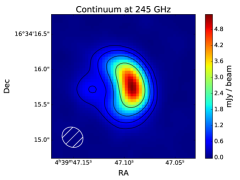
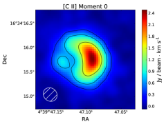
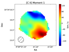
Figure 1: The clean image and moments of J0439+1634 observed with ALMA. Upper Left: the continuum; Upper Right: the zeroth moment of [C ii] emission; Lower Left and Lower Right: the first and second moments of the [C ii] emission. The data are cleaned using Briggs weighting with $\text{robust}=0.5$. In the first and second moment maps, we only show pixels that have integrated flux signal-to-noise ratio larger than 10. Contours in the continuum map are at $20\sigma$, $40\sigma$, $80\sigma$ and $160\sigma$ levels, where $\sigma$ is the flux error per beam estimated using an annulus with $1^{\prime\prime}<r<2^{\prime\prime}$. Similarly, Contours in the [C ii] moment 0 map are at $10\sigma$, $20\sigma$ and $40\sigma$ levels. The moment 1 map shows rotation-like ordered motion.

We reduce the ALMA data using the Common Astronomy Software Applications (CASA) version 5.6.1 (McMullin et al., 2007). We use the task UVCONTSUB to fit a linear function to the line-free channels, which models the continuum, and subtract the continuum model to obtain the line-only visibility. We then use the continuum data to perform phase self-calibration and apply the self-calibration model to the line-only data. We clean the continuum and line data with the CASA task TCLEAN using Briggs weighting, setting robust $=0.5$. The synthesized beam has a size of $0\farcs 31\times 0\farcs 27$ and a position angle of $39.4$ degrees. Figure 1 shows the cleaned image of the dust continuum and the zeroth, first, and second moments of the [C ii] emission. J0439+1634 is clearly resolved as an arc-like shape, which is typical for lensed galaxies. The zeroth moment (integrated flux) of the [C ii] line is more extended than the continuum flux. The first moment (mean velocity map) shows ordered motion.

We extract the continuum and [C ii] fluxes of J0439+1634 with a $2\farcs 0$ diameter aperture, which gives $S_{\text{245 GHz}}=16.0\pm 0.1\text{ mJy}$ for the continuum and $F_{\text{[C\,{\sc ii}]}}=14.5\pm 0.2\text{ Jy km s}^{-1}$ for the integrated [C ii] flux. We also fit a Gaussian profile to the [C ii] line using the CASA task SPECFIT. The [C ii] line is centered at $252.7744\pm 0.0011$ GHz with an FWHM of $270.0\pm 2.8\text{ km s}^{-1}$, which gives a redshift $z_{\text{[C\,{\sc ii}]}}=6.51871\pm 0.00003$. In the rest of the paper, we set 252.7744 GHz as the rest frequency for [C ii]. Figure 2 shows the extracted [C ii] line profile, which is well-fitted by a Gaussian function and shows no evidence for an excess redshifted or blueshifted component.

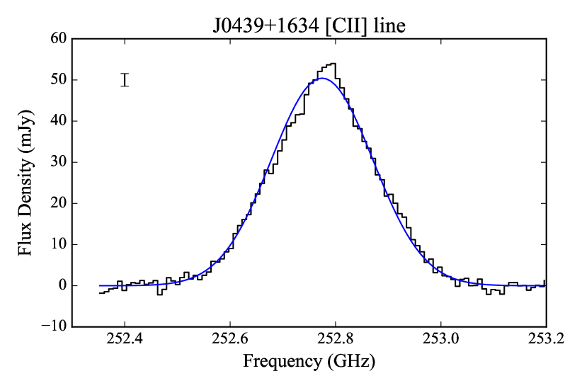
Figure 2: The [C ii] line profile of J0439+1634, extracted from the cleaned image using a $2^{\prime\prime}$ diameter aperture. The error bar in the upper left corner shows the uncertainty of the flux density. The red line presents the best-fit Gaussian profile, which has a FWHM of $270.0\pm 2.8\text{ km s}^{-1}$ and a central frequency of $252.7744\pm 0.0011$ GHz.

3 Lensing Model

We use VISILENS (Spilker et al., 2016) to model the visibility of J0439+1634. VISILENS is a parameterized lens modeling tool for interferometry data. In short, VISILENS models the $uv-$plane response of a lens system and obtains the posterior distributions of model parameters using Markov Chain Monte Carlo (MCMC).

Table 1: Lens model parameters

	Default			ALMA only
Parameters	lens	Continuum	[C ii]	lens	Continuum	[C ii]
Redshift	[0.67]	[6.5187]	[6.5187]	[0.67]	[6.5187]	[6.5187]
$\Delta\text{RA}~{}(^{\prime\prime})$	$0.459\pm 0.002$	$0.236\pm 0.003$	$0.235\pm 0.002$	$0.409\pm 0.004$	$0.222\pm 0.005$	$0.220\pm 0.005$
$\Delta\text{Dec}~{}(^{\prime\prime})$	$-0.050\pm 0.001$	$-0.019\pm 0.001$	$-0.017\pm 0.001$	$-0.058\pm 0.002$	$-0.019\pm 0.003$	$-0.017\pm 0.003$
Mass $(M_{\odot})$	[$2.06\times 10^{10}$]	-	-	$(1.95\pm 0.03)\times 10^{10}$	-	-
$e$	[0.65]	$0.409\pm 0.011$	$0.376\pm 0.020$	$0.641\pm 0.007$	$0.362\pm 0.016$	$0.347\pm 0.021$
PA (deg)	[94.58]	$-6.9\pm 1.2$	$-0.6\pm 1.7$	$99.75\pm 0.34$	$4.9\pm 1.5$	$3.4\pm 2.2$
Flux	-	$3.46\pm 0.04$	$4.15\pm 0.10$	-	$3.18\pm 0.07$	$4.16\pm 0.10$
$R_{\text{eff}}~{}(^{\prime\prime})$	-	$0.136\pm 0.002$	$0.233\pm 0.006$	-	$0.131\pm 0.002$	$0.235\pm 0.007$
$n$	-	$1.71\pm 0.06$	$0.82\pm 0.05$	-	$1.58\pm 0.05$	$0.91\pm 0.05$
$\mu$	-	$4.53\pm 0.05$	$3.44\pm 0.05$	-	$4.90\pm 0.10$	$3.45\pm 0.05$

Note. — The quantities in the square brackets are fixed. For the lens galaxy, Fan et al. (2019) use Einstein radius instead of mass. Here we follow the convention in VISILENS. The redshift and the mass of the lens galaxy are degenerate, and the lens parameters in this table gives the same lensing model as Fan et al. (2019). Besides, note that the uncertainties only include statistical errors, and do not take into account the systematic errors introduced by the model choice (see Section 3.5 for more discussion).

3.1 Building the Lensing Model

Fan et al. (2019) built the lensing model of J0439+1634 based on the HST image, where they used a singular isothermal ellipsoid (SIE; e.g., Kormann et al., 1994) to describe the mass distribution of the lens galaxy. In their fiducial model, the lensing galaxy has a high ellipticity $(e=0.65)$, lies at the west side of the quasar, and generates three quasar images. The position, the ellipticity, and the position angle of the modeled lens galaxy are consistent with the observed HST optical image.

The HST images have spatial resolution of $\sim 0\farcs 075$, which is several times better than the current ALMA data. We thus adopt the lens mass distribution from the fiducial model in Fan et al. (2019). Specifically, we use an SIE to describe the lens galaxy. The Einstein radius, ellipticity, and position angle of the SIE are fixed to the values in the fiducial HST model, while the position of the lens is left free, which accounts for any pointing offsets between HST and ALMA. Because the continuum has a higher signal-to-noise ratio (SNR), we first fit the continuum to obtain the best-fit lens position, then apply the lens position when fitting the [C ii] emission. We use a Sérsic profile to describe the source, both for the continuum and the [C ii] line emission. This model is referred to as the default model in this paper.

For comparison, we also build an alternative model, hereafter referred as the “ALMA-only” model, in which we leave all parameters free when fitting the ALMA data and do not use any information from the HST observations. Again, we use an SIE to describe the lens galaxy and a Sérsic profile to describe the source emission, both for the continuum and the [C ii] line. We first fit the continuum to obtain the best-fit values of the lens parameters, then apply these values when fitting the [C ii] line.

Figure 3 shows the fitting result of the default model, and Figure 4 illustrates the ALMA-only model. Table 1 summarizes the best-fit parameters for both models. Despite tiny differences in details, the two models give the same overall lensing structure. Because the HST images have better resolution, we use the default model to derive the properties of J0439+1634 from this point on. We will discuss the systematic errors introduced by the choice of the model in Section 3.5.

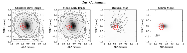
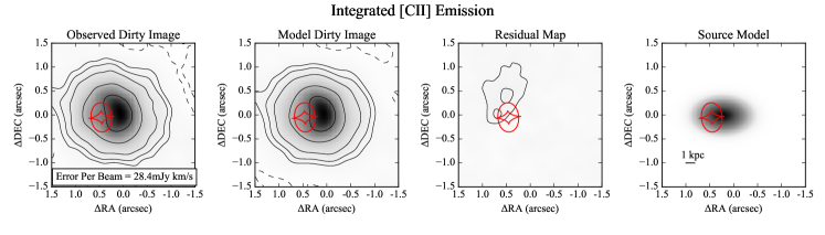
Figure 3: The default lensing model of J0439+1634 based on ALMA and HST observations. Upper Panel: the continuum model. From left to right: the observed dirty image with natural weighting, the modeled dirty image with natural weighting, the residual image, and the source model. Contours in the observed and model images are $-10\sigma$, $-5\sigma$, $5\sigma$, $10\sigma$, $20\sigma$, $50\sigma$, $100\sigma$, $200\sigma$ and $400\sigma$ levels, where $1\sigma$ equals to the “error per beam” in the observed image. Contours in the residual image are $-5\sigma$, $5\sigma$, $10\sigma$, $15\sigma$, $20\sigma$ and $25\sigma$ levels. In all images, dashed black lines are negative contours and solid black lines are positive ones. The red line marks the caustics of the lens. When fitting the continuum, we fix the lens parameters, except the position, to the fiducial model in Fan et al. (2019). Lower Panel: Same as the upper panel, but for [C ii] emission. The lens parameters in the [C ii] fitting are fixed to the best-fit values in the continuum model.

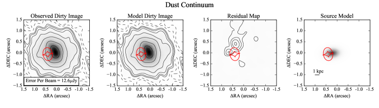
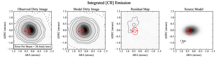
Figure 4: Same as Figure 3, but for the ALMA-only lensing model. We first fit the continuum visibility with all parameters left free, then fit the [C ii] emission with lens galaxy parameters fixed to the best-fit values in the continuum model. This ALMA-only model and the default model in Figure 3 are nearly identical.

In addition to the fiducial model, Fan et al. (2019) raise two alternative models, in which the lens mass distribution differs significantly from the fiducial model and produces either double or quadruple quasar images. See Figure 4 in Fan et al. (2019) for more information. The alternative models do not provide suitable fits to the ALMA data. We conclude that the fiducial HST model has the correct lensing configuration.

3.2 Dust Continuum

The upper panel of Figure 3 shows the best-fit dust continuum in the default model. As described in Section 3.1, in the default model, we fix the deflector galaxy mass distribution to the fiducial model in Fan et al. (2019) which is based on HST imaging, and fit the quasar host galaxy emission in ALMA data as a Sérsic profile. The dirty images are generated with natural weighting to enhance the SNR. The dust continuum of J0439+1634 can be well-fitted by a single Sérsic profile, with a reduced $\chi^{2}=1.035$. The best-fit Sérsic index is $1.71\pm 0.06$ and the half-light radius is $0\farcs 136\pm 0\farcs 002$ ($0.74\pm 0.01$ kpc), suggesting a compact, exponential-disk-like profile. (See Section 4.1 for further discussion.) The overall magnification is $4.53\pm 0.05$ when averaged over the entire galaxy. Compared to the fiducial HST model, the position of the optical quasar deviates from the continuum center by $0\farcs 014$. The typical astrometric error for ALMA is about 5% of the resolution, which translates to $\sim 0\farcs 015$ given a beam size of $\sim 0\farcs 3$ (the ALMA technical handbook, e.g., Cortes et al., 2020). The positions of the optical quasar and the host galaxy are thus consistent.

The residual map shows some statistically significant structures. The peak of these structures is $4.9\%$ of the peak in the observed dirty image. We expect such features given that we use a simple SIE + Sérsic model and the SNR of the data is high (with natural weighting, the peak SNR in the dirty image is $\sim 600$). When we add a Gaussian profile to the source model, where we allow the Gaussian profile to have negative flux, the flux of the Gaussian profile converges to zero within the error. We thus argue that the structures in the residual image cannot be explained by a single bump or void in the source galaxy. The structures might result from an over-simplification of the lens and source model.

3.3 Integrated [C ii] Flux

The lower panel of Figure 3 shows the best-fit result of the [C ii] emission in the default model, and Table 1 shows the parameters of [C ii] line observations. The reduced $\chi^{2}$ of the best-fit model is $1.014$. The best-fit [C ii] emission has a Sérsic index of $0.82\pm 0.05$, consistent with an exponential $(n=1)$ profile, and a half-light radius of $0\farcs 233\pm 0\farcs 006$ $(1.27\pm 0.03\text{ kpc})$. The position and the ellipticity of the integrated [C ii] emission are consistent with those of the dust continuum within $2\sigma$, while the [C ii] line has a smaller Sérsic index and larger half-light radius. This difference suggests that the [C ii] line is more diffuse than the dust, as shown in the clean images. The overall magnification of the [C ii] emission is $3.44\pm 0.05$, which is smaller than that of the dust continuum, mainly because the [C ii] profile is more diffused.

Similar to the continuum, a Sérsic profile captures the major features of the [C ii] emission. The residual image of the [C ii] emission is similar to the continuum residual. The peak in the residual is $8.1\%$ of the peak in the dirty image.

3.4 [C ii] Kinematics

Figure 1 suggests that the host galaxy of J0439+1634 has an ordered, rotation-like velocity field. We thus fit the [C ii] emission using an axisymmetric rotating thin disk, following the method described in Neeleman et al. (2019). In short, we set up parameterized models for the flux distribution, the mean velocity field, and the velocity dispersion field. We then use VISILENS to calculate the lensed [C ii] emission and the $uv-$plane response in each velocity channel. We obtain the best-fit model parameters by minimizing the residual of the visibility in all channels. To keep maximum flexibility, we do not constrain the parameters using the Sérsic model for the integrated [C ii] flux. We assume a Sérsic profile for the flux distribution and apply various forms for the rotation curve and the velocity dispersion profile. However, all of these models return large residuals and unphysical best-fit parameters. We thus conclude that J0439+1634 cannot be described by an axisymmetric rotating thin disk.

The main reason for the poor fit is the apparent misalignment between the major axis of the flux distribution and the velocity gradient. For an axisymmetric rotation disk, the major axis and the velocity gradient should be in the same direction. In contrast, the major axis of the flux distribution of J0439+1634 is roughly aligned east-to-west (Figure 3, right panel), while the velocity gradient is roughly north-to-south (Figure 1). To further investigate this problem, we estimate the source-plane flux distribution using a simple inverse ray-tracing method. Specifically, we reconstruct the source (i.e., un-lensed) data cube on a grid with a pixel size of $0\farcs 04$. Using the overall [C ii] magnification $\mu_{\text{[C\,{\sc ii}]}}=3.44$, we estimate the average source-plane resolution to be $\sim\sqrt{0\farcs 31\times 0\farcs 27}/\sqrt{3.44}=0\farcs 156$ for the [C ii] emission. A pixel size of $0\farcs 04$ gives a super-Nyquist sampling, which helps to resolve the regions with higher magnification than the average value. We then trace all the pixels in the image-plane data cube (i.e., the clean image) to the source plane according to the default lensing model. If more than one image-plane pixels are traced to the same source-plane pixel, these image pixels are averaged. This simple method captures the main features of the quasar host galaxy without expensive pixelized lensing reconstruction.

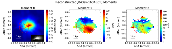
Figure 5: The reconstructed source-plane moments. From left to right: the reconstructed zeroth, first, and second moments. The coordinates are relative to the phase center. The images have pixel sizes of $0\farcs 04$ (0.22 kpc). The black cross marks the center of the [C ii] emission from the default lensing model. The red line illustrates the lensing caustics. The moment 2 map has some pixels missing due to low SNR which leads to mathematical errors (i.e., getting a squared root of a negative value). The lower-right corner of the left panel shows the output when performing the inverse ray-tracing analysis to a beam on the image plane which locates at the flux peak. The “reconstructed” beam has a size of $0\farcs 26\times 0\farcs 09$ and is a rough estimate of the source-plane beam shape.

We generate source-plane moment maps using the reconstructed data cube. When calculating the first and the second moments, we only include pixels that have integrated flux SNR larger than $10$. Figure 5 shows the reconstructed moments, which confirm the overall picture of J0439+1634: a regular profile for the integrated emission (moment 0) and a rotation-like mean velocity field (moment 1). The major axis of moment 0 is significantly offset from the velocity gradient in the moment 1 map, confirming the argument we made with the lensed image. Another hint is the structures in the moment 2 map. For a rotating thin disk, we expect a peak at the center of the moment 2 map due to the beam smearing effect where the line-of-sight velocity gradient is large. This peak is not seen in Figure 5; instead, the moment 2 map has complex structures, which indicate complicated velocity field in the host galaxy.

The lower-right corner of the reconstructed moment 0 map illustrates the output when we perform the inverse ray-tracing analysis to an image-plane beam located at the image-plane flux peak. This “reconstructed” beam is a rough estimate of the beam shape on the source plane. The source-plane beam has a size of $0\farcs 26\times 0\farcs 09$, which further illustrates that a source-plane pixel size of $0\farcs 04$ is appropriate.

Note that the blue and red wings in the moment 1 map are located outside of the caustics, which means that they are not multiply-imaged. For these areas, the effect of gravitational lensing on the observations is equivalent to shrinking the beam size and applying some image distortions. As such, the inverse ray-tracing reconstruction can capture the structure of the velocity field, especially in the blue and red wings. In Figure 6, we illustrate the position-velocity plot of J0439+1634, generated using the reconstructed moment 0 and moment 1. We extract the velocities along the black line, which connects the pixels with the maximum and minimum moment 1 value (i.e., the red and blue peaks). The position-velocity plot clearly shows a rotation-like feature. The velocity rises at $r\lesssim 1\text{ kpc}$ and flattens beyond this radius. The maximum rotation velocity is roughly $v_{\text{max}}\sin(i)=130\text{ km s}^{-1}$ where $i$ is the inclination angle of the rotation axis, and the velocity is measured out to $r_{\text{max}}=2\text{ kpc}$.

In addition to the rotation-like feature, the position-velocity plot contains another component with low velocity $(|v|\lesssim 50\text{ km s}^{-1},\text{marked by the yellow box})$. We mark pixels that contribute to this feature with black dots in the moment 1 map in Figure 6. These pixels either lie inside the caustics, which means that they are multiply imaged, and have complicated lens-mapping function, or have low signal and large errors. The simple inverse ray-tracing method will fail for these areas, and this component is likely an artifact. If it is physical, it might reflect some complex structures in the host galaxy, which can be resolved in the upcoming high-resolution ALMA observations. Possible scenarios include minor mergers and clumpy star-formation regions. In any case, this structure only contributes $\sim 10\%$ of the total flux, and the rotation-like feature dominates the velocity field.

J0439+1634 has a rotation-like velocity field, but cannot be described by an axisymmetric rotating thin disk. It is likely that the [C ii] emission is not axisymmetric and/or that the host galaxy has a thick geometry. Both cases are common for high-redshift sgalaxies (e.g., Pensabene et al., 2020; Förster Schreiber & Wuyts, 2020). Specifically, many star-forming galaxies at $z\gtrsim 2$ have velocity dispersion $\sigma\gtrsim 45\text{ km s}^{-1}$ and show thick geometry (for a recent review, see Förster Schreiber & Wuyts, 2020). For J0439+1634, we can estimate its velocity dispersion using the regions where the rotation curve has flattened. The moment 2 map suggests that these regions have $\sigma\sim 70\text{ km s}^{-1}$, which means that a thick geometry is likely.

Fitting a non-axisymmetric model and/or a thick disk model requires high spatial resolution, and our data cannot put a strong constraint on these models. In future work, we will perform pixelized lensing reconstruction and detailed dynamical modeling once the high-resolution ALMA observations are carried out (Project 2018.1.00566.S, PI: Fan).

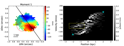
Figure 6: Left: The moment 1 map. The black line illustrates the axis used to extract the position-velocity diagram. The axis connects the pixels with the maximum and minimum moment 1 value (i.e., the blue peak and the red peak). The black dots mark the pixels that contributes to the minor feature in the position-velocity diagram (marked by the yellow box in the right panel). The red curve marks the caustics. Right: The position-velocity diagram. The diagram contains a rotation-like feature and a minor feature marked by the yellow box. The two cyan asterisks correspond to the value we adopt for the maximum velocity and the corresponding radius: $v_{\text{max}}\sin(i)=130\text{ km s}^{-1}$ and $r_{\text{max}}=2\text{ kpc}$.

3.5 Systematic Uncertainties

We first consider the systematic errors in the fluxes and sizes of the continuum and the [C ii] emission. The main source of systematic errors is that the SIE + Sérsic lensing model is over-simplified. As a result, there are positive clumps in the residual images in Figure 3. The flux of the clumps is much smaller than the the flux calibration error and is negligible in the error analysis. Properly modeling the structures in the residual images requires expensive pixelized modeling of the source flux and the lens mass (e.g., Hezaveh et al., 2016), which is beyond the scope of this paper.

We then consider the systematic uncertainties in the source-plane reconstruction in Section 3.4. The major uncertainty is the beam-smearing effect. The source-plane resolution is $\sim 0\farcs 15$ $(\sim 0.8\text{ kpc})$. In this study, we focus on the maximum rotation velocity rather than detailed velocity field structure. Beam-smearing effects have little influence on our main result, because (1) the blue and red peaks are only singly imaged, and (2) the rotation velocity flattens at $r\gtrsim 1\text{ kpc}$, so the central, low-velocity area does not influence the edge at $r_{\text{max}}=2\text{ kpc}$ where we measure the maximum velocity. Similar methods have been adopted by recent studies to measure the rotation velocity of lensed galaxies (e.g., Cheng et al., 2020).

4 Physical Properties of J0439+1634

4.1 Dust Continuum and [C ii] Emission

The host galaxy of J0439+1634 has a regular Sérsic profile, both for the continuum and [C ii] emission. The Sérsic index is close to one, which suggests that J0439+1634 is more similar to an exponential disk than a de-Vaucouleurs bulge with $n=4$. The [C ii] line profile is also well-described by a single-peaked Gaussian profile, with no excess of blueshifted or redshifted components. The smooth structures in the moment maps and the position-velocity plot disfavor the scenario of a close, on-going major merger. In addition, no other objects are detected within the ALMA field of view $(\sim 12^{\prime\prime})$. These results suggest that J0439+1634 is not an on-going major merger and does not exhibit significant outflow features in the [C ii] velocity field. However, it is possible that J0439+1634 is a minor merger or a remnant of a recent major merger.

Yang et al. (2019b) measure the far-infrared (FIR) to centimeter-wavelength spectral energy distribution (SED), as well as the CO, [C i], [C ii], [O i], and $\text{H}_{2}\text{O}$ emission lines of J0439+1634. Their NOrthern Extended Millimeter Array (NOEMA) observation gives $z_{\text{[C\,{\sc ii}]}}=6.5188\pm 0.0002$, $F_{\text{[C\,{\sc ii}]}}=11.7\pm 0.8\text{ Jy km s}^{-1}$, $\text{FWHM}_{\text{[C\,{\sc ii}]}}=328.1\pm 18.0\text{ km s}^{-1}$, and $S_{\text{239 GHz}}=14.0\pm 0.1\text{ mJy}$. The typical flux calibration uncertainty is $\sim 15\%$ for NOEMA and $\sim 10\%$ for ALMA. The continuum and [C ii] line fluxes reported in Section 2 are consistent with those in Yang et al. (2019b). The difference in the FWHM of the [C ii] line is about 3$\sigma$.

Based on these measurements, Yang et al. (2019b) calculate the infrared luminosities, emission line luminosities, star formation rate, dust mass, and gas mass without correcting for the lensing magnification. We refer the reader to Yang et al. (2019b) for the details of how these properties are calculated. In this work, with spatially resolved ALMA images, we calculate the de-lensed values of these quantities. For [C ii]-based quantities, we apply the magnification of [C ii] emission, $\mu_{\text{[C\,{\sc ii}]}}=3.44$; for FIR-based quantities, we apply the continuum magnification, $\mu_{\text{cont}}=4.53$. In addition, we apply the continuum magnification to the CO-based molecular gas mass, assuming that the dust continuum traces the molecular gas. The results are listed in Table 2. Similar to other high-redshift quasars (e.g., Walter et al., 2009; Decarli et al., 2018; Wang et al., 2019a), J0439+1634 is hosted by a gas-rich ultra luminous infrared galaxy (ULIRG) with intense star formation activity, with a TIR luminosity of $\sim 10^{13}L_{\odot}$.

Table 2: De-lensed Physical Properties of J0439+1634

[C ii]-Based Properties
$L_{\text{[C\,{\sc ii}]}}(L_{\odot})$	$(3.5\pm 0.3)\times 10^{9}$
$L^{\prime}_{\text{[C\,{\sc ii}]}}(\text{K km s}^{-1}\text{pc}^{2})$	123456789012345 $(1.7\pm 0.1)\times 10^{10}$
$M_{\text{C}^{+}}(M_{\odot})$	($1.1\pm 0.1)\times 10^{7}$
$\text{SFR}_{\text{{[C\,{\sc ii}]}}}(M_{\odot}\text{ year}^{-1})$	$\sim 233\sim 1398$
Other properties
$L_{\text{FIR}}(L_{\odot})$	$(7.5\pm 0.4)\times 10^{12}$
$L_{\text{TIR}}(L_{\odot})$	$(1.06\pm 0.04)\times 10^{13}$
$\text{SFR}_{\text{TIR}}(M_{\odot}\text{ year}^{-1})$	$1.56\times 10^{3}$
$M_{\text{dust}}(M_{\odot})$	$4.9\pm 0.2\times 10^{8}$
$M_{\text{H}_{2},\text{CO}}(M_{\odot})$	$1.19\times 10^{10}$

Note. — These values are calculated according to Table 1 in Yang et al. (2019b). We apply $\mu=\mu(\text{[C\,{\sc ii}]})=3.44$ for [C ii]-based quantities and $\mu=\mu(\text{continuum})=4.53$ for the other quantities. FIR luminosity includes flux in rest-frame $42.5-122.5~{}\mu$m, and TIR luminosity includes flux in rest-frame $8-1000~{}\mu$m. The uncertainties only reflect statistical errors.

One interesting aspect of the [C ii] emission is the so-called “[C ii] deficit.” In systems with high FIR surface brightness ($\Sigma_{\text{FIR}}\gtrsim 10^{11}L_{\odot}\text{ kpc}^{-2}$; e.g., Díaz-Santos et al., 2017; Herrera-Camus et al., 2018), the [C ii]-to-FIR ratio decreases with $\Sigma_{\text{FIR}}$. This relation has been observed in many different systems, including nebulae in the Milky Way (for example, the Orion Nebula; e.g., Goicoechea et al., 2015), local luminous infrared galaxies (LIRGs) and ULIRGs (e.g., Díaz-Santos et al., 2013), high-redshift submillimeter galaxies (SMGs) (e.g., Oteo et al., 2016; Spilker et al., 2016; Litke et al., 2019) and quasars (e.g., Decarli et al., 2018; Neeleman et al., 2019). The underlying mechanism of the [C ii] deficit might be complex. Some plausible scenarios include: (1) In regions with higher surface density, most carbon atoms are in the form of CO molecules rather than $\text{C}^{+}$ ions (Narayanan & Krumholz, 2017); (2) [C ii] might become optically thick at high surface density (Luhman et al., 1998); (3) Large FIR surface brightness indicates strong dust absorption of the UV radiation, which is the main heating source of [C ii] emission (Herrera-Camus et al., 2018); (4) [C ii] emission might be saturated in warm gas (Muñoz & Oh, 2016).

With spatially resolved data, we can investigate the [C ii] deficit in different regions of J0439+1634. Using the continuum and [C ii] model in Figure 3, we measure the [C ii] and FIR flux of J0439+1634 in four regions. The $n^{\text{th}}$ region is defined as $n\times R_{\text{eff}}<R<(n+1)\times R_{\text{eff}}$, where $n=0,1,2,3$, and $R_{\text{eff}}=0\farcs 136$ is the half-light radius of the continuum emission. All regions have the same center, ellipticity, and position angle as the continuum emission. The widths of the rings are close to the average source-plane resolution of $0\farcs 15$. The flux calibration error ($\sim 15\%$) is the dominant source of uncertainty, and we ignore other uncertainties.

Figure 7 illustrates the position of J0439+1634 on the [C ii]$/$FIR$-\Sigma_{\text{FIR}}$ plot. We include $z\gtrsim 6$ quasars from the literature for comparison. Specifically, three quasars from Shao et al. (2017) and Wang et al. (2019c) have spatially resolved measurements. We also include LIRGs from the Great Observatories All-sky LIRG Survey (GOALS) sample (Díaz-Santos et al., 2013), SMGs at $4.5<z<6.5$ (Riechers et al., 2013; Neri et al., 2014; Gullberg et al., 2018), and resolved regions of a gravitationally lensed SMG at $z=5.7$, SPT0346 (Litke et al., 2019). Similar to other objects with high-resolution data, different regions in J0439+1634 tightly follow the [C ii] deficit. Our result thus suggests that the [C ii] deficit is related to physical processes on $\lesssim 1\text{ kpc}$ scales, i.e., it reflects the properties of the local ISM rather than the entire galaxy.

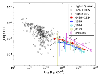
Figure 7: The [C ii]-FIR ratio versus FIR surface brightness plot for resolved regions in J0439+1634, local LIRGs in the GOALS sample (Díaz-Santos et al., 2013), quasars at $z\gtrsim 6$ (Wang et al., 2013; Venemans et al., 2016, 2017; Shao et al., 2017; Decarli et al., 2018; Izumi et al., 2018; Wang et al., 2019a, c; Venemans et al., 2020), and $4.5<z<6.5$ SMGs (Riechers et al., 2013; Neri et al., 2014; Gullberg et al., 2018; Litke et al., 2019). Besides J0439+1634, three quasars and an SMG in this plot have resolved measurements, including J1319 (Shao et al., 2017), J0129, and J1044 (Wang et al., 2019c), and SPT0346 (Litke et al., 2019). The points representing different regions in one object are connected by a line.

4.2 Host Galaxy Dynamics

Using the maximum line-of-sight velocity $v_{\text{max}}\sin(i)=130\text{ km s}^{-1}$ and the corresponding radius $r_{\text{max}}=2\text{ kpc}$, we estimate the dynamical mass within $r_{\text{max}}$ for J0439+1634, $M_{\text{dyn}}\sin^{2}(i)=7.9\times 10^{9}M_{\odot}$. We report in Table 2 the $\text{H}_{2}$ mass of J0439+1634, $M_{\text{H}_{2},\text{CO}}(M_{\odot})=1.19\times 10^{10}M_{\odot}$, which gives a gas-mass fraction of $1.5\times\sin^{2}(i)$. The gas-mass fraction is high except for very low inclinations.

Although the host galaxy of J0439+1634 has a regular shape and a rotation-like velocity field, we show in Section 3.4 that this galaxy is not an axisymmetric thin disk. Plausible scenarios include (1) the emission in the galaxy is not axisymmetric, which can happen when the star-forming regions are not evenly distributed on the disk, or (2) the host galaxy has a “thick” geometry (e.g., a spheroid) and is not a thin disk. The upcoming high-resolution ALMA data will reveal small-scale structures that might distinguish these models. Here we briefly discuss the implications of the thick disk model, since the moment 2 map indicates that a thick geometry is likely (Section 3.4).

A thick disk with a large velocity dispersion has a non-negligible turbulent pressure gradient which needs to be considered when estimating the dynamical mass. Following the discussion in Förster Schreiber & Wuyts (2020), we estimate the circular velocity of the host galaxy, $v_{c}$:

$$v_{c}^{2}=v_{\text{max}}^{2}+2\sigma^{2}\times(r/R_{d})$$ (1)

which is related to the dynamical mass by $M_{\text{dyn}}(r)=v_{c}^{2}r/G$, where $R_{d}$ is the scaling radius of the exponential disk (i.e., $I(r)\propto e^{-r/R_{d}}$). Applying $v_{\text{max}}=130/\sin(i)\text{ km s}^{-1}$, $r=2\text{ kpc}$, $\sigma=70\text{ km s}^{-1}$ and $R_{d}=0.8$ kpc according to the best-fit [C ii] model in Section 3.3 yields

$$v_{c}^{2}=\left[\frac{130\text{ km/s}}{\sin(i)}\right]^{2}+(160\text{ km/s})^{2}$$ (2)

which suggests that, in the thick-disk model, the contribution of velocity dispersion is significant. However, the velocity dispersion should be taken as an upper limit given the beam smearing effect. It is hard to correct the beam smearing effect under the current resolution; as such, we still use $M_{\text{dyn}}\sin^{2}(i)=7.9\times 10^{9}M_{\odot}$ in the rest of this paper. This result illustrates the need of careful modeling with high-resolution data when measuring the dynamical mass of high-redshift quasar host galaxies.

Pensabene et al. (2020) analyzes the archival ALMA data of 32 quasars to model their kinematics, where ten quasars at $z>5.7$ are found to have rotation-like velocity fields. Among these ten quasars, three have a significantly misaligned flux major axis and velocity gradient. This result suggests that complicated kinematics are common in high-redshift quasars and that high-resolution observations are crucial to understanding high-redshift quasar host galaxies.

5 A Maximum Starburst System With Oversized Black Hole at Cosmic Dawn

5.1 A Maximum Star Forming Rotating System

Our analysis shows that the host galaxy of J0439+1634 is a compact ULIRG with vigorous star formation. Assuming that the dust continuum traces the SFR surface density (SFRD), we estimate the SFRD within the continuum half-light radius to be $\Sigma_{\text{SFR}}\approx 800M_{\odot}\text{ year}^{-1}\text{ kpc}^{-2}$. Such a high $\Sigma_{\text{SFR}}$ is close to the highest SFRD values seen in the universe ($\sim 10^{3}M_{\odot}\text{ year}^{-1}\text{kpc}^{-2}$; e.g., Walter et al., 2009) and approaches the Eddington-limit of star formation (Thompson et al., 2005). In addition, we estimate the maximum SFR proposed by Elmegreen (1999), where the gas is assumed to collapse on a free-fall timescale, $t_{\text{ff}}=\sqrt{2R^{3}/GM}=1.06\sin(i)\times 10^{7}$ year. The maximum possible SFR is $\epsilon M_{\text{gas}}/t_{\text{ff}}$, where $\epsilon$ is the efficiency of gas turning into stars. This argument suggests that J0439+1634 has a maximum possible SFR of $\epsilon\sin^{-1}(i)\times 1.12\times 10^{3}M_{\odot}\text{ year}^{-1}$ within a radius of $R<2\text{ kpc}$. For any reasonable inclination angle $(i\gtrsim 5^{\circ})$, a high star formation efficiency is required $(\epsilon\gtrsim 0.1)$. Our analysis suggests that J0439+1634 is forming stars at the maximum possible rate.

The rich gas reservoir and the vigorous star formation of J0439+1634 could be a remnant of a recent major merger or strong cold gas inflow (e.g., Dekel et al., 2009). The major merger remnant scenario is promising because it provides a natural explanation to the misalignment between the major axis and the velocity gradient, i.e., the star-formation regions are not yet evenly distributed in the rotating disk. Under the current resolution, small-scale structures will get smoothed out, and the flux distribution mimics a Sérsic profile. Upcoming high-resolution ALMA data could reveal these possible structures.

5.2 SMBH-Host Co-evolution

Fan et al. (2019) measures the SMBH mass of J0439+1634 to be $M_{\text{BH}}=(4.29\pm 0.60)\times 10^{8}M_{\odot}$, which gives $M_{\text{BH}}/M_{\text{dyn}}=0.055\sin^{2}(i)$. Assuming J0439+1634 follows the local relation in Kormendy & Ho (2013) yields $M_{\text{BH}}/M_{\text{host}}=0.005$. A face-on rotation model with inclination $i=17^{\circ}$ moves J0439+1634 onto the local $M_{\text{BH}}-M_{\text{host}}$ relation, and a fiducial inclination angle of $i=60^{\circ}$ yields $M_{\text{BH}}/M_{\text{host}}=0.04$. This result is similar to that in many high-redshift quasars (e.g., Venemans et al., 2017; Decarli et al., 2018; Wang et al., 2019a), which have $M_{\text{BH}}/M_{\text{host}}$ several times higher than the local relation.

With the SMBH mass and the observed central velocity dispersion, we estimate the size of the SMBH’s sphere of influence:

$$r_{h}=\frac{GM_{\text{BH}}}{\sigma^{2}}.$$ (3)

Both the image-plane moment 2 (Figure 1) and the reconstructed source-plane moment 2 (Figure 5) show roughly constant velocity dispersion across the galaxy. We thus adopt the median value of the source-plane moment 2 map, $\sigma_{\text{med}}=94\text{ km s}^{-1}$, which gives $r_{h}=0.18\text{ kpc}$. The most extended configuration of ALMA delivers a resolution of $\sim 0\farcs 02$. For the region near the SMBH, we apply the magnification of the optical quasar from Fan et al. (2019), $\mu_{\text{quasar}}=51.3$. An image-plane resolution of $0\farcs 02$ thus corresponds to a source-plane resolution of $\sim 2.8\text{ mas}$ $(\sim 16\text{ pc})$. Thus, high-resolution ALMA observations will allow us to sample the SMBH’s sphere of influence well and to measure the mass of the SMBH directly via gas kinematics.

Direct measurement of SMBH mass has been possible only at low-redshift (for a review, see Kormendy & Ho, 2013). For most high-redshift quasars, SMBH masses are measured based on the empirical relation between the continuum luminosity and the broad line region size (e.g., Vestergaard & Peterson, 2006), which has only been calibrated at $z\lesssim 2$. J0439+1634 thus provides a unique opportunity to calibrate the SMBH mass measurement at high redshift.

6 Conclusions

We present ALMA observations of a gravitationally lensed quasar at $z=6.52$, J0439+1634. We model the dust-continuum, the [C ii] emission, and the velocity field of the host galaxy. Our main conclusions are:

1. The ALMA observations demonstrate that the three-image fiducial model in Fan et al. (2019) based on HST observations of the quasar is correct, ruling out the alternative models considered in Fan et al. (2019) . The default lensing model gives an overall magnification of $4.53\pm 0.05$ and $3.44\pm 0.05$ for the continuum and [C ii] emission of the host galaxy, respectively. The average source-plane resolution is $\sim 0\farcs 15$ $(\sim 0.8\text{ kpc})$.

2. J0439+1634 is a compact ULIRG well-described by a compact Sérsic profile. The Sérsic index is close to one for both the continuum and [C ii] emission. The resolved regions in J0439+1634 follow the “[C ii] deficit,” suggesting that the deficit is related to the sub-kpc properties of the ISM.

3. J0439+1634 has a rotation-like velocity field, but it cannot be well described as an axisymmetric rotating thin disk. The maximum line-of-sight rotation velocity is $v_{\text{max}}\sin(i)=130\text{ km s}^{-1}$, with the inclination angle $i$ unconstrained. The dynamical mass within $2\text{ kpc}$ is $7.9\times 10^{9}\sin^{-2}(i)M_{\odot}$. J0439+1634 is likely a gas-rich galaxy with a high gas-mass fraction.

4. J0439+1634 is forming stars at the maximum possible rate. The star-formation rate surface density of J0439+1634 approaches the largest value seen in the universe and the Eddington limit.

5. The SMBH-to-dynamical mass ratio of J0439+1634 is $0.055\times\sin^{2}(i)$, which suggests that J0439+1634 is likely to host an oversized SMBH compared to local relations. The size of the sphere of influence is $0.18\text{ kpc}$. The most extended configuration of ALMA will resolve the sphere of influence and allow us to measure the SMBH mass directly using the gas kinematics.

Our lensing model incorporates the major features of J0439+1634 detected under low resolution ALMA data. Future high-resolution ALMA observations with higher-resolution, combined with pixelized lens modeling, will reveal more detailed structures in the foreground lens and quasar host galaxy. Specifically, as discussed in Section 5.2, the resolution around the SMBH will reach $\sim 16\text{ pc}$ within the SMBH sphere of influence. The power of gravitational lensing makes J0439+1634 a valuable object for a case study, which will provide crucial and previously inaccessible information about the coevolution of SMBHs and their hosts at $z>6$.

References

- Bañados et al. (2016) Bañados, E., Venemans, B. P., Decarli, R., et al. 2016, ApJS, 227, 11, doi: 10.3847/0067-0049/227/1/11
- Bañados et al. (2018) Bañados, E., Venemans, B. P., Mazzucchelli, C., et al. 2018, Nature, 553, 473, doi: 10.1038/nature25180
- Bañados et al. (2019) Bañados, E., Novak, M., Neeleman, M., et al. 2019, ApJ, 881, L23, doi: 10.3847/2041-8213/ab3659
- Beelen et al. (2006) Beelen, A., Cox, P., Benford, D. J., et al. 2006, ApJ, 642, 694, doi: 10.1086/500636
- Bolatto et al. (2013) Bolatto, A. D., Wolfire, M., & Leroy, A. K. 2013, ARA&A, 51, 207, doi: 10.1146/annurev-astro-082812-140944
- Cheng et al. (2020) Cheng, C., Cao, X., Lu, N., et al. 2020, ApJ, 898, 33, doi: 10.3847/1538-4357/ab980b
- Cortes et al. (2020) Cortes, P. C., Remijan, A., Biggs, A., et al. 2020, ALMA Technical Handbook, ALMA Doc. 8.4, ver. 1.0. https://almascience.nrao.edu/documents-and-tools/cycle8/alma-technical-handbook
- Decarli et al. (2018) Decarli, R., Walter, F., Venemans, B. P., et al. 2018, ApJ, 854, 97, doi: 10.3847/1538-4357/aaa5aa
- Dekel et al. (2009) Dekel, A., Birnboim, Y., Engel, G., et al. 2009, Nature, 457, 451, doi: 10.1038/nature07648
- Díaz-Santos et al. (2013) Díaz-Santos, T., Armus, L., Charmandaris, V., et al. 2013, ApJ, 774, 68, doi: 10.1088/0004-637X/774/1/68
- Díaz-Santos et al. (2017) —. 2017, ApJ, 846, 32, doi: 10.3847/1538-4357/aa81d7
- Elmegreen (1999) Elmegreen, B. G. 1999, ApJ, 517, 103, doi: 10.1086/307200
- Fan et al. (2019) Fan, X., Wang, F., Yang, J., et al. 2019, ApJ, 870, L11, doi: 10.3847/2041-8213/aaeffe
- Förster Schreiber & Wuyts (2020) Förster Schreiber, N. M., & Wuyts, S. 2020, ARA&A, 58, 661, doi: 10.1146/annurev-astro-032620-021910
- Goicoechea et al. (2015) Goicoechea, J. R., Teyssier, D., Etxaluze, M., et al. 2015, ApJ, 812, 75, doi: 10.1088/0004-637X/812/1/75
- Gullberg et al. (2018) Gullberg, B., Swinbank, A. M., Smail, I., et al. 2018, ApJ, 859, 12, doi: 10.3847/1538-4357/aabe8c
- Herrera-Camus et al. (2018) Herrera-Camus, R., Sturm, E., Graciá-Carpio, J., et al. 2018, ApJ, 861, 94, doi: 10.3847/1538-4357/aac0f6
- Hezaveh et al. (2016) Hezaveh, Y. D., Dalal, N., Marrone, D. P., et al. 2016, ApJ, 823, 37, doi: 10.3847/0004-637X/823/1/37
- Inoue et al. (2020) Inoue, K. T., Matsushita, S., Nakanishi, K., & Minezaki, T. 2020, ApJ, 892, L18, doi: 10.3847/2041-8213/ab7b7e
- Izumi et al. (2018) Izumi, T., Onoue, M., Shirakata, H., et al. 2018, PASJ, 70, 36, doi: 10.1093/pasj/psy026
- Izumi et al. (2019) Izumi, T., Onoue, M., Matsuoka, Y., et al. 2019, PASJ, 71, 111, doi: 10.1093/pasj/psz096
- Jiang et al. (2016) Jiang, L., McGreer, I. D., Fan, X., et al. 2016, ApJ, 833, 222, doi: 10.3847/1538-4357/833/2/222
- Kormann et al. (1994) Kormann, R., Schneider, P., & Bartelmann, M. 1994, A&A, 284, 285
- Kormendy & Ho (2013) Kormendy, J., & Ho, L. C. 2013, ARA&A, 51, 511, doi: 10.1146/annurev-astro-082708-101811
- Leipski et al. (2014) Leipski, C., Meisenheimer, K., Walter, F., et al. 2014, ApJ, 785, 154, doi: 10.1088/0004-637X/785/2/154
- Litke et al. (2019) Litke, K. C., Marrone, D. P., Spilker, J. S., et al. 2019, ApJ, 870, 80, doi: 10.3847/1538-4357/aaf057
- Luhman et al. (1998) Luhman, M. L., Satyapal, S., Fischer, J., et al. 1998, ApJ, 504, L11, doi: 10.1086/311562
- Marshall et al. (2020) Marshall, M. A., Mechtley, M., Windhorst, R. A., et al. 2020, arXiv e-prints, arXiv:2007.13859. https://arxiv.org/abs/2007.13859
- Matsuoka et al. (2016) Matsuoka, Y., Onoue, M., Kashikawa, N., et al. 2016, ApJ, 828, 26, doi: 10.3847/0004-637X/828/1/26
- Matsuoka et al. (2018a) Matsuoka, Y., Iwasawa, K., Onoue, M., et al. 2018a, ApJS, 237, 5, doi: 10.3847/1538-4365/aac724
- Matsuoka et al. (2018b) Matsuoka, Y., Onoue, M., Kashikawa, N., et al. 2018b, PASJ, 70, S35, doi: 10.1093/pasj/psx046
- Matsuoka et al. (2019) Matsuoka, Y., Iwasawa, K., Onoue, M., et al. 2019, ApJ, 883, 183, doi: 10.3847/1538-4357/ab3c60
- McMullin et al. (2007) McMullin, J. P., Waters, B., Schiebel, D., Young, W., & Golap, K. 2007, in Astronomical Society of the Pacific Conference Series, Vol. 376, Astronomical Data Analysis Software and Systems XVI, ed. R. A. Shaw, F. Hill, & D. J. Bell, 127
- Mechtley et al. (2012) Mechtley, M., Windhorst, R. A., Ryan, R. E., et al. 2012, ApJ, 756, L38, doi: 10.1088/2041-8205/756/2/L38
- Muñoz & Oh (2016) Muñoz, J. A., & Oh, S. P. 2016, MNRAS, 463, 2085, doi: 10.1093/mnras/stw2102
- Murphy et al. (2011) Murphy, E. J., Condon, J. J., Schinnerer, E., et al. 2011, ApJ, 737, 67, doi: 10.1088/0004-637X/737/2/67
- Narayanan & Krumholz (2017) Narayanan, D., & Krumholz, M. R. 2017, MNRAS, 467, 50, doi: 10.1093/mnras/stw3218
- Neeleman et al. (2019) Neeleman, M., Bañados, E., Walter, F., et al. 2019, ApJ, 882, 10, doi: 10.3847/1538-4357/ab2ed3
- Neri et al. (2014) Neri, R., Downes, D., Cox, P., & Walter, F. 2014, A&A, 562, A35, doi: 10.1051/0004-6361/201322528
- Oteo et al. (2016) Oteo, I., Ivison, R. J., Dunne, L., et al. 2016, ApJ, 827, 34, doi: 10.3847/0004-637X/827/1/34
- Pensabene et al. (2020) Pensabene, A., Carniani, S., Perna, M., et al. 2020, A&A, 637, A84, doi: 10.1051/0004-6361/201936634
- Riechers et al. (2009) Riechers, D. A., Walter, F., Bertoldi, F., et al. 2009, ApJ, 703, 1338, doi: 10.1088/0004-637X/703/2/1338
- Riechers et al. (2013) Riechers, D. A., Bradford, C. M., Clements, D. L., et al. 2013, Nature, 496, 329, doi: 10.1038/nature12050
- Rigopoulou et al. (2018) Rigopoulou, D., Pereira-Santaella, M., Magdis, G. E., et al. 2018, MNRAS, 473, 20, doi: 10.1093/mnras/stx2311
- Schreiber et al. (2018) Schreiber, C., Elbaz, D., Pannella, M., et al. 2018, A&A, 609, A30, doi: 10.1051/0004-6361/201731506
- Shao et al. (2017) Shao, Y., Wang, R., Jones, G. C., et al. 2017, ApJ, 845, 138, doi: 10.3847/1538-4357/aa826c
- Shao et al. (2019) Shao, Y., Wang, R., Carilli, C. L., et al. 2019, ApJ, 876, 99, doi: 10.3847/1538-4357/ab133d
- Spilker et al. (2016) Spilker, J. S., Marrone, D. P., Aravena, M., et al. 2016, ApJ, 826, 112, doi: 10.3847/0004-637X/826/2/112
- Spilker et al. (2020) Spilker, J. S., Phadke, K. A., Aravena, M., et al. 2020, ApJ, 905, 85, doi: 10.3847/1538-4357/abc47f
- Thompson et al. (2005) Thompson, T. A., Quataert, E., & Murray, N. 2005, ApJ, 630, 167, doi: 10.1086/431923
- Venemans et al. (2019) Venemans, B. P., Neeleman, M., Walter, F., et al. 2019, ApJ, 874, L30, doi: 10.3847/2041-8213/ab11cc
- Venemans et al. (2016) Venemans, B. P., Walter, F., Zschaechner, L., et al. 2016, ApJ, 816, 37, doi: 10.3847/0004-637X/816/1/37
- Venemans et al. (2012) Venemans, B. P., McMahon, R. G., Walter, F., et al. 2012, ApJ, 751, L25, doi: 10.1088/2041-8205/751/2/L25
- Venemans et al. (2013) Venemans, B. P., Findlay, J. R., Sutherland, W. J., et al. 2013, ApJ, 779, 24, doi: 10.1088/0004-637X/779/1/24
- Venemans et al. (2015) Venemans, B. P., Bañados, E., Decarli, R., et al. 2015, ApJ, 801, L11, doi: 10.1088/2041-8205/801/1/L11
- Venemans et al. (2017) Venemans, B. P., Walter, F., Decarli, R., et al. 2017, ApJ, 837, 146, doi: 10.3847/1538-4357/aa62ac
- Venemans et al. (2018) Venemans, B. P., Decarli, R., Walter, F., et al. 2018, ApJ, 866, 159, doi: 10.3847/1538-4357/aadf35
- Venemans et al. (2020) Venemans, B. P., Walter, F., Neeleman, M., et al. 2020, ApJ, 904, 130, doi: 10.3847/1538-4357/abc563
- Vestergaard & Peterson (2006) Vestergaard, M., & Peterson, B. M. 2006, ApJ, 641, 689, doi: 10.1086/500572
- Walter et al. (2009) Walter, F., Riechers, D., Cox, P., et al. 2009, Nature, 457, 699, doi: 10.1038/nature07681
- Wang et al. (2019a) Wang, F., Wang, R., Fan, X., et al. 2019a, ApJ, 880, 2, doi: 10.3847/1538-4357/ab2717
- Wang et al. (2017) Wang, F., Fan, X., Yang, J., et al. 2017, ApJ, 839, 27, doi: 10.3847/1538-4357/aa689f
- Wang et al. (2019b) Wang, F., Yang, J., Fan, X., et al. 2019b, ApJ, 884, 30, doi: 10.3847/1538-4357/ab2be5
- Wang et al. (2008) Wang, R., Carilli, C. L., Wagg, J., et al. 2008, ApJ, 687, 848, doi: 10.1086/591076
- Wang et al. (2010) Wang, R., Carilli, C. L., Neri, R., et al. 2010, ApJ, 714, 699, doi: 10.1088/0004-637X/714/1/699
- Wang et al. (2013) Wang, R., Wagg, J., Carilli, C. L., et al. 2013, ApJ, 773, 44, doi: 10.1088/0004-637X/773/1/44
- Wang et al. (2019c) Wang, R., Shao, Y., Carilli, C. L., et al. 2019c, ApJ, 887, 40, doi: 10.3847/1538-4357/ab4d4b
- Weiß et al. (2005) Weiß, A., Downes, D., Henkel, C., & Walter, F. 2005, A&A, 429, L25, doi: 10.1051/0004-6361:200400085
- Willott et al. (2015) Willott, C. J., Bergeron, J., & Omont, A. 2015, ApJ, 801, 123, doi: 10.1088/0004-637X/801/2/123
- Yang et al. (2019a) Yang, J., Wang, F., Fan, X., et al. 2019a, AJ, 157, 236, doi: 10.3847/1538-3881/ab1be1
- Yang et al. (2019b) Yang, J., Venemans, B., Wang, F., et al. 2019b, ApJ, 880, 153, doi: 10.3847/1538-4357/ab2a02
- Yang et al. (2020) Yang, J., Wang, F., Fan, X., et al. 2020, ApJ, 897, L14, doi: 10.3847/2041-8213/ab9c26