Accumulative Iterative Codes Based on Feedback

Abstract

The Accumulative Iterative Code (AIC) proposed in this work is a new error correcting code for channels with feedback. AIC sends the information message to the receiver in a number of transmissions, where the initial transmission contains the uncoded message and each subsequent transmission informs the receiver about the locations of the errors that corrupted the previous transmission. Error locations are determined based on the forward channel output, which is made available to the transmitter through the feedback channel.

AIC achieves arbitrarily low error rates, thereby being suitable for applications demanding extremely high reliability. In the same time, AIC achieves spectral efficiencies very close to the channel capacity in a wide range of signal-to-noise ratios even for transmission of short information messages.

I Introduction

Achieving wired-like communication performances through wireless connections is an extremely ambitious goal. Nonetheless, some of the most advanced applications of future mobile cellular networks require levels of reliability and latency similar to their wired counterparts. In the industrial automation domain [1], for example, there is increasing interest for providing wireless connectivity to devices involved in the assistance and supervision of production processes, and even in real-time motion control of production machinery. In real-time motion control, the controller application and the controlled machinery are connected through radio links. All the messages exchanged over the radio links have to be properly secured and the probability of two consecutive packet errors must be made negligible. According to [1], a single packet error may be tolerable, whereas two consecutive packet errors may cause damages to the controlled machines and cause interruptions to the production processes.

In conventional transmission systems, high reliability is obtained by Error Correction Coding (ECC). Conventional ECC methods already provide reliable transmission with Spectral Efficiency (SE) very close to the channel capacity. However, the only way for obtaining reliable transmission and capacity-approaching SE at the same time is by transmission of long codewords. With short codes, the achievable SE is significantly smaller than the channel capacity, as predicted by the accurate analytical characterization in [2]. In practice, even the best error correction codes, such as the 3GPP New Radio (NR) Low-Density Parity Check (LDPC) codes and polar codes [3], are unable to provide capacity-approaching SE and high reliability at the same time [4]. The gap between channel capacity and SE of short-codeword transmission is remarkably large for low signal-to-noise ratios (SNRs). For example, on the Additive White Gaussian Noise (AWGN) channel with SNR smaller than 0 dB, the largest achievable SE by any 128-bit code at BLock Error Rate (BLER) of $10^{-4}$ is less than half the channel capacity [4].

Conventional ECC methods do not send any feedback information. However, as the majority of contemporary communication systems have two-way links, feedback channels are available in most cases. It is therefore natural to seek improvements over conventional ECC by making use of feedback. A well-known information-theoretic result [5, Thm. 7.12.1 and Sec. 9.6] stipulates that feedback does not increase the capacity of memoryless channels. Even in the most favorable case – instantaneous noiseless feedback – the channel capacity remains unchanged. This means that the largest rate at which reliable transmission is possible is the same regardless of whether feedback is available or not. Nevertheless, digital communication research has shown that usage of feedback potentially brings significant advantages in terms of improved reliability. Improving the reliability yields decreased BLER, thereby producing increased spectral efficiency.

The improved reliability of feedback-based codes has been shown for the first time in the pioneering work of Schalkwjik and Kailath [6]. The authors of [6] developed a code and a corresponding iterative encoding procedure for channels with noiseless feedback where the transmitter sends an information message in an initial uncoded transmission followed by a number of subsequent transmissions containing corrections for the initial transmission. Correction signals are calculated based on the information fed back to the transmitter through a feedback channel. Transmission of corrections continues for a predefined number of times. After the last transmission, the receiver delivers in its output an accurate replica of the transmitted information. The error performance analysis of the Schalkwjik-Kailath (SK) code reveals that the error probability has a doubly-exponential decay with the codeword length $N$, as shown by the following equation [7]:

$$P_{w}^{\rm(SK)}<\exp\left(-A\times 2^{2N(C-R)}\right).$$ (1)

Here, $P_{w}^{\rm(SK)}$ is the probability that the SK decoder delivers in its output a decoded message containing errors, $A$ is a SNR-dependent term, $N$ is the codeword length, $C$ is the channel capacity and $R$ is the code rate. In comparison, the error probability of conventional ECC exhibits an exponential decay with $N$, as shown by the following equation [8]:

$$P_{w}^{\rm(ECC)}<\exp\left(-NE(R)\right).$$ (2)

Here, $E(R)$ is the reliability function [8], also called the error exponent. $E(R)$ is a monotonically decreasing function of $R$. The faster decay with $N$ of the feedback codes’ error probability predicted by (1) is the main motivation behind our interest in this kind of codes as it suggests that feedback codes potentially attain lower error probabilities already with short codewords.

The SK code promises to achieve remarkable performance compared to conventional ECC. However, its sensitivity to finite-precision numerical computations precludes practical implementations. To overcome the above shortcomings, several variations and enhancements have been developed subsequently based on similar principles. A concise account of those solutions can be found in [9, Ch. 17].

One of the most recent developments aimed at overcoming the SK shortcomings is the code architecture based on deep recurrent neural networks called Deepcode [10]. Deepcode sends the uncoded information message in an initial transmission and subsequently generates a sequence of parity-check symbols based on the information message and on the past forward-channel outputs. Forward channel outputs are fed back to the encoder through a feedback channel. Neural network weights are obtained by jointly training the encoder and decoder according to a conventional machine-learning procedure. Performance evaluation in [10] show that Deepcode achieves significantly lower error rates compared to conventional ECC. However, there is a remaining gap between SE and the channel capacity.

Among the proposed solutions, the Compressed Error Cancellation (CEC) framework [11] is one of the most attracting approaches as it combines optimum reliability with the proven ability to achieve a rate arbitrarily close to the channel capacity. As a further benefit, CEC has low encoding/decoding complexity. Similar as SK, CEC operates according to an iterative encoding procedure. The initial transmission delivers the information message. A number of subsequent transmissions are performed in order to send updates produced by the encoder based on the last transmission and on the channel outputs obtained through feedback. The updates are produced in two steps: a source coding step followed by a precoding step. Source coding produces a compressed word based on the last transmitted sequence and on the corresponding received sequence, which is made available to the transmitter through the feedback channel. Precoding divides the source-coded bits into segments of fixed length and maps each segment to a real integer in a given range (e.g., $\{-M,\ldots,M\}$) through the cumulative distribution of the forward channel input sequence. In that way, the symbols in the precoded sequence are distributed according to the forward-channel capacity achieving distribution. Performance evaluations in [11] show that CEC performs reliable transmission of long information messages – 1 Mbit length – at a rate approaching the capacity of the AWGN channel with 0 dB SNR within a very small gap. However, as it will be shown later in the performance evaluations, CEC transmission of short messages (here, ”short” refers to messages of length 100 bits or less) achieves significantly smaller data rates compared to the channel capacity.

The Accumulative Iterative Code (AIC) of this paper builds upon the findings of [11] to develop a new solution that significantly reduces the rate-capacity gap for short codeword transmission and, at the same time, is of practical interest as its building blocks are often found in most radio communication systems. Major novelties of AIC are the following:

• Usage of Huffman source coding. Huffman coding is preferred over other source coding methods because it produces the lowest expected codeword length in its output.

• Usage of conventional modulations on the forward channel. Conventional modulations are preferred to the precoding of [11] as they are already present in most radio communication systems, they allow simple implementation and achieve rates close to channel capacity in wide SNR ranges.

• Feedback based on quantized Log-Likelihood Ratios (LLRs). Sending the LLRs of transmitted bits on the feedback channel makes AIC independent of the modulation. Moreover, LLR quantization keeps the feedback data rate contained. The LLR quantization method here considered is optimal in the sense that, for given number of quantization levels, the quantization thresholds are determined so as to maximize the mutual information of modulator input and quantizer output.

Performance evaluations show that AIC achieves SE close to channel capacity and arbitrarily low error rate at the same time, thereby providing significant gains compared to conventional coding methods. The rest of the paper is organized as follows: Sec. II describes AIC, the structure of encoder an decoder, and the encoding and decoding procedures. Sec. III shows the results of performance evaluation. with conventional ECC. Final observations and conclusions are given in Sec. IV.

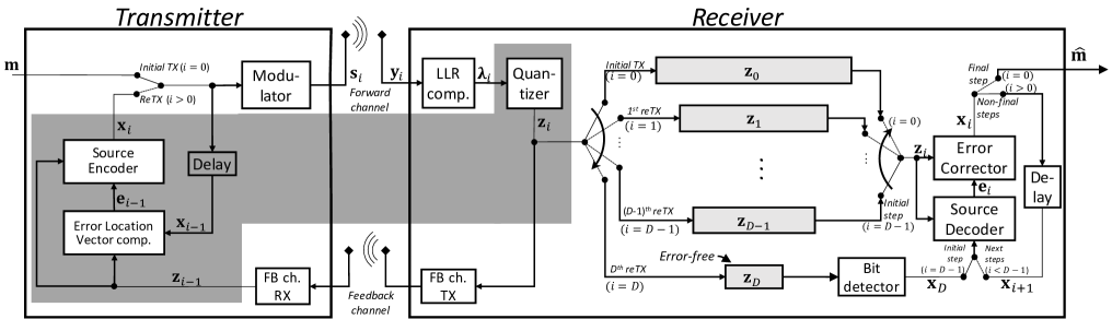
Figure 1: AIC transmission system. The encoder is highlighted by a grey-shaded background.

II The Accumulative Iterative Code

Figure 1 shows the block scheme of AIC transmission system where the encoder is highlighted by a grey-shaded background. The AIC encoder is split between transmitter and receiver. The encoder’s transmitter component and receiver component interact with each other by exchanging signals through the forward channel and the feedback channel. In each iteration, the encoder computes an error location vector ($\mathbf{e}_{i-1}$ in Figure 1) which contains the locations of errors in the last forward transmission. Vector $\mathbf{e}_{i-1}$ is computed based on the previously transmitted sequence $\mathbf{x}_{i-1}$ and on the information obtained through the feedback channel ($\mathbf{z}_{i-1}$ in Figure 1). The error location vector is source-coded so as to generate a source-coded error location vector ($\mathbf{x}_{i}$ in Figure 1). The vector $\mathbf{x}_{i}$ is sent through the forward channel so as to make error correction possible in the receiver. However, as the received source-coded vector may again be corrupted by errors, a further iteration is needed in order to inform the decoder about error locations. The feedback channel is assumed to be reliable – the information transmitted on the feedback channel is not corrupted by any errors. In the receiver, Log-Likelihood Ratios (LLRs) of the received signals are quantized and stored in memory buffers. The Quantized LLRs (QLLRs) are also fed back to the transmitter through the feedback channel.

The AIC transmitter keeps sending error words on the forward channel until an error-free forward transmission occurs or until a maximum number of iterations is reached. When an error-free forward transmission occurs, the transmitter informs the receiver that decoding can be performed. Start of decoding can be signaled to the decoder, e.g., by sending an acknowledgment (ACK) message through a control channel. If a maximum number of iterations is reached and no error-free forward transmissions occurred, the transmitter notifies the receiver (e.g., by sending a negative acknowledgment – NACK – message through the control channel) that transmission of the information message failed.

After reception of the ACK message, the decoder starts the decoding process. In a first decoding step, the decoder determines the source-coded error location vector that was transmitted in the last iteration ($\mathbf{x}_{D}$ in Figure 1). In subsequent decoding iterations, the decoder determines the error location vectors ($\mathbf{e}_{i}$ in Figure 1) by source-decoding the vectors $\mathbf{x}_{i+1}$ and applies corresponding corrections. In a final step, the decoder obtains the decoded message $\mathbf{\hat{m}}$.

The above encoding and decoding procedures are described in detail in the subsections below.

II-A Encoding Procedure

The encoding procedure consists of a number of iterations, where in each iteration the transmitter and receiver exchange signals through the forward and feedback channels. In the initial iteration, the transmitter sends a $K$-bit information message $\mathbf{m}=(m_{1},\ldots,m_{K})$ on the forward channel; in subsequent iterations, the transmitter sends source-coded error location vectors $\mathbf{x}_{i},i=0,\ldots,D$, where $\mathbf{x}_{i}=(x_{i,1},\ldots,x_{i,N_{i}})$. is the transmitted word in the $i^{\rm th}$ iteration and $N_{i}$ is its length. For convenience, we define ${\bf x}_{0}\triangleq{\bf m}$ and $N_{0}\triangleq K$.

The message $\mathbf{m}$ and the source coded vectors $\mathbf{x}_{i},i=0,\ldots,D$, are transmitted on the forward channel using conventional modulations. In the $i^{\rm th}$ iteration, the modulator generates a sequence $\mathbf{s}_{i}=(s_{i,1},\ldots,s_{i,L_{i}})$, where $L_{i}=\left\lceil N_{i}/Q\right\rceil$ and $Q$ is the modulation order. Each element of $\mathbf{s}_{i}$ is obtained by mapping a group of $Q$ consecutive bits (hereafter called a $Q$-tuple) of $\mathbf{x}_{i}$ to a complex signal selected from a given set $\Psi=\{\psi_{1},\ldots,\psi_{2^{Q}}\}$ through a one-to-one labeling map $\mu_{Q}:\{0,1\}^{Q}\to{\Psi}$.

The received sequence is obtained as follows:

$$\mathbf{y}_{i}=\mathbf{s}_{i}+{\boldsymbol{\nu}}_{i}$$ (3)

where ${\boldsymbol{\nu}}_{i}$ represents noise, interference and distortions introduced by the forward channel.

Based on the received sequence $\mathbf{y}_{i}$, the encoder computes a sequence of LLRs of transmitted bits ${\boldsymbol{\lambda}}_{i}=(\lambda_{i,1},\ldots,\lambda_{i,N_{i}})$ as follows:

$$\lambda_{i,n} = \log\frac{P(x_{i,n}=0\mid\mathbf{y}_{i})}{P(x_{i,n}=1\mid\mathbf{y}_{i})}$$ (4)

$$= \log{\frac{\sum_{t\in{\Psi}_{0}^{p(n)}}{P(y_{i,q(n)}\mid s_{i,q(n)}=t)}}{\sum_{t\in{\Psi}_{1}^{p(n)}}{P(y_{i,q(n)}\mid s_{i,q(n)}=t)}}}$$ (5)

where $n=1,\ldots,N_{i}$, $P(\cal E)$ denotes the probability of event $\cal E$, $q(n)$ is the position in the sequence $\mathbf{s}_{i}$ of the modulation signal that carries $x_{i,n}$ and $p(n)$ is the position of $x_{i,n}$ in the $Q$-tuple that produced that modulation signal. ${\Psi}_{b}^{p(n)}$ denotes the subset of the signals of $\Psi$ whose label has value $b$ in position $p(n)$, where $b\in\{0,1\}$.

Each LLR in the above sequence is quantized so as to obtain a sequence of QLLRs $\mathbf{z}_{i}=(z_{i,1},\ldots,x_{i,N_{i}})$ as follows:

$$z_{i,n}=Q_{\boldsymbol{\theta}^{*}}(\lambda_{i,n})$$ (6)

where $\boldsymbol{\theta}^{*}=(\theta_{0}^{*},\ldots,\theta_{R-1}^{*},\theta_{R}^{*}=+\infty)$ is a vector of non-negative quantization thresholds arranged in increasing order, i.e.:

$$\theta_{0}^{*}<\theta_{1}^{*}<\ldots<\theta_{R}^{*}$$ (7)

and $Q_{\boldsymbol{\theta}^{*}}$ is a function that maps an arbitrary real value $\lambda$ to an integer value in the set $\{0,\pm 1,...,\pm R\}$ as follows:

$$Q_{\boldsymbol{\theta}^{*}}(\lambda)\triangleq\left\{\begin{array}[]{rcl}+r&\textrm{if}&\theta_{r-1}^{*}\leq\lambda<\theta_{r}^{*}\\ 0&\textrm{if}&|\lambda|<\theta_{0}^{*}\\ -r&\textrm{if}&-\theta_{r}^{*}<\lambda\leq-\theta_{r-1}^{*}\end{array}\right.,r=1,\ldots,R.$$ (8)

The optimal quantization thresholds vector – denoted as $\boldsymbol{\theta}^{*}$ – is obtained by maximizing the amount of information that is transferred from the modulator input to the quantizer output through the forward channel. Assuming that $X$ is a Random Variable (RV) representing the modulator input and $Z$ is a RV representing the LLR quantizer output, the vector $\boldsymbol{\theta}^{*}$ is given by

$$\begin{split}\boldsymbol{\theta}^{*}=\arg\max_{\boldsymbol{\theta}}\sum_{u\in\{0,1\}}\sum_{v\in\{0,\pm 1,\ldots,\pm R\}}p_{uv}(\boldsymbol{\theta})P_{X}(u)\log\frac{p_{uv}(\boldsymbol{\theta})}{P_{Z}(v)}\end{split}$$ (9)

where the probabilities $p_{uv}(\boldsymbol{\theta})$ are defined as follows:

$$p_{uv}(\boldsymbol{\theta})= P(Z=v\mid X=u;\boldsymbol{\theta}),$$

$$u\in\{0,1\},v\in\{0,\pm 1,\ldots,\pm R\}.$$ (10)

Moreover, we assume uniform input distribution and thus

$$P_{X}(u)\triangleq P(X=u)=1/2,u\in\{0,1\}$$ (11)

and probabilities $P_{Z}(v)$ are obtained as follows:

$$P_{Z}(v)\triangleq P(Z=v)=\sum_{u\in\{0,1\}}{p_{uv}(\boldsymbol{\theta})P_{X}(u)}.$$ (12)

By taking into account quantization as mathematically modeled by equations (6) and (8), equation (II-A) yields:

$$p_{uv}(\boldsymbol{\theta})\!=\!\left\{\!\begin{array}[]{ll}\!P(\lambda_{i,n}\!\in\![\theta_{v-1},\theta_{v})\!\mid\!x_{i,n}=u)&(v>0)\\ \!P(\lambda_{i,n}\!\in\!(-\theta_{0},\theta_{0})\!\mid\!x_{i,n}=u)&(v=0)\\ \!P(\lambda_{i,n}\!\in\!(-\theta_{-v},-\theta_{-v-1}]\!\mid\!x_{i,n}=u)&(v<0)\end{array}\right.$$ (13)

The following example illustrates how (13) can be computed in a practical case – BPSK signals transmitted on the AWGN channel. The procedure in the example can be straightforwardly extended to Gray-mapped QPSK signals on AWGN, as the in-phase and quadrature components of QPSK can be treated as independent BPSK-modulated signals.

Example. For BPSK signals corrupted by AWGN, (5) can be simplified as follows:

$$\lambda_{i,n}=\frac{2}{\sigma_{\nu}^{2}}y_{i,n}.$$ (14)

By combining (13) and (14), after few algebraic transformations we obtain

$$p_{uv}(\boldsymbol{\theta})\!=\!\left\{\!\begin{array}[]{lc}\!\int_{\frac{\sigma_{\boldsymbol{\nu}}^{2}}{2}\theta_{|v|-1}-\phi(v)\mu_{\rm BPSK}(u)}^{\frac{\sigma_{\boldsymbol{\nu}}^{2}}{2}\theta_{|v|}-\phi(v)\mu_{\rm BPSK}(u)}{f_{\boldsymbol{\nu}}(y)}{\rm d}y&(v\neq 0)\\ \!\int_{-\frac{\sigma_{\boldsymbol{\nu}}^{2}}{2}\theta_{0}-\mu_{\rm BPSK}(u)}^{\frac{\sigma_{\boldsymbol{\nu}}^{2}}{2}\theta_{0}-\mu_{\rm BPSK}(u)}{f_{\boldsymbol{\nu}}(y)}{\rm d}y&(v=0)\end{array}\right.$$ (15)

where $\mu_{\rm BPSK}(u)$ is the conventional BPSK mapping, defined as follows

$$\mu_{\rm BPSK}(u)\triangleq 1-2u,\quad u\in\{0,1\}.$$ (16)

and $\phi(v)$ is the sign function: $\phi(v)\triangleq v/|v|$. The function $f_{\boldsymbol{\nu}}(y)$ is the well-known Gaussian pdf with zero mean and variance $\sigma_{\boldsymbol{\nu}}^{2}$:

$$f_{\boldsymbol{\nu}}(y)=\frac{1}{\sqrt{2\pi}\sigma_{\boldsymbol{\nu}}}e^{-y^{2}/(2\sigma_{\boldsymbol{\nu}}^{2})}.$$ (17)

The above example showed how to compute the probabilities $p_{uv}(\boldsymbol{\theta})$ for a given modulation format based on the channel noise pdf $f_{\boldsymbol{\nu}}(y)$. For those cases where $f_{\boldsymbol{\nu}}(y)$ is not known, the probabilities (II-A) have to be calculated by Monte Carlo simulation.

The QLLRs sequence $\mathbf{z}_{i}$ computed according to (6) is stored in receiver memory buffers and sent back to the transmitter through the feedback channel. Based on the QLLRs sequence ${\bf z}_{i}$ and on the corresponding transmitted word $\mathbf{x}_{i}$, the transmitter determines the error location vector $\mathbf{e}_{i}=(e_{i,1},\ldots,e_{i,N_{i}})$ as follows:

$$\mathbf{e}_{i}=\mathbf{\bar{x}}_{i}\oplus\mathbf{x}_{i}$$ (18)

where $\oplus$ denotes bit-wise modulo-2 sum and the vector $\mathbf{\bar{x}}_{i}=(\bar{x}_{i,1},\ldots,\bar{x}_{i,N_{i}})$ is obtained as follows:

$$\bar{x}_{i,n}=\left\{\begin{array}[]{rcl}0&\textrm{if}&{z}_{i,n}>0\\ 1&\textrm{if}&{z}_{i,n}<0\end{array}\right.,n=1,\ldots,N_{i}.$$ (19)

Thus, $\bar{x}_{i,n}$ is the most likely value of the transmitted bit $x_{i,n}$ based on the corresponding QLLR $z_{i,n}$.

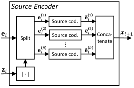
Figure 2: Source encoder. $|\cdot|$ denotes absolute value.

The vector $\mathbf{e}_{i}$ is source-coded so as to obtain a source-coded error location vector $\mathbf{x}_{i}$. The source encoder is shown in Figure 2. Source coding of error location vectors is performed according to the following steps:

1. Splitting. The error location vector $\mathbf{e}_{i}$ is split into $R$ subvectors $\mathbf{e}_{i}^{(r)},r=1,\ldots,R$, where $\mathbf{e}_{i}^{(r)}$ contains the elements of $\mathbf{e}_{i}$ whose corresponding QLLRs have absolute value $r$;

2. Source coding. Each subvector $\mathbf{e}_{i}^{(r)}$ is source-coded so as to obtain a source coded subvector $\mathbf{\tilde{e}}_{i}^{(r)}$.

3. Concatenation. The source coded sub-vectors $\mathbf{\tilde{e}}_{i}^{(r)}$ are concatenated so as to obtain a source coded error location vector $\mathbf{x}_{i+1}$.

When $\theta_{0}>0$, the source encoder further appends to $\mathbf{x}_{i+1}$ the bits of $\mathbf{x}_{i}$ whose corresponding QLLR is 0.

The source coding method we adopt is the Huffman method [5]. For a given positive integer $H$, the Huffman encoder divides its input vector $\mathbf{e}_{i}^{(r)}$ into $\lceil\ell(\mathbf{e}_{i}^{(r)})/H\rceil$ non-overlapping segments $f_{k}$ of $H$ consecutive bits. When $\ell(\mathbf{e}_{i}^{(r)})$ is not an integer multiple of $H$, zeros are appended to $\mathbf{e}_{i}^{(r)}$ until the length becomes multiple of $H$. Assuming that the bits of $\mathbf{e}_{i}^{(r)}$ are statistically independent and take value ’1’ with probability $\pi_{r}$, the probability of a segment $f_{k}$ is given by:

$$P(f_{k})=\pi_{r}^{\boldsymbol{\omega}(f_{k})}(1-\pi_{r})^{H-\omega(f_{k})}$$ (20)

where $\omega(f_{k})$ denotes the number of ’1’s in $f_{k}$. Based on the above probabilities (20), the source encoder codebook is determined by the well known Huffman method [5]. Once the codebook has been determined, the Huffman encoder maps each segment $f_{k}$ to a corresponding codeword $\tilde{f}_{k}$ from the codebook and produces a corresponding source-coded subvector $\mathbf{\tilde{e}}_{i}^{(r)}$ by concatenating the codewords $\tilde{f}_{k}$ as follows:

$$\tilde{\mathbf{e}}_{i}^{(r)}=[\tilde{f}_{1},\ldots,\tilde{f}_{\lceil\ell(\mathbf{e}_{i}^{(r)})/H\rceil}].$$ (21)

In the sequel, we will discuss how the probabilities $\pi_{r}$ of (20) are calculated.

We recall that a ’1’ in $\mathbf{e}_{i}^{(r)}$ indicates that a forward transmission error occurred in a corresponding bit of $\mathbf{x}_{i}$. According to the definition of LLR (4), a forward transmission error occurs if (i) the quantizer produces a negative QLLR when the corresponding transmitted bit is ’0’, or (ii) the quantizer produces a positive QLLR when the corresponding transmitted bit is ’1’. The above events have the following probabilities:

$$\pi_{r,0} = P(Z<0\mid X=0,|Z|=r)$$ (22)

$$\pi_{r,1} = P(Z>0\mid X=1,|Z|=r).$$ (23)

In general, the error probabilities (22) and (23) are not equal. However, the source encoder treats both probabilities in the same way, that is, it does not distinguish whether a bit error corresponds to a transmitted ’1’ or ’0’. Thus, it is necessary to make sure that there is a contained difference between $\pi_{r,0}$ and $\pi_{r,1}$, that is:

$$\pi_{r,0}\cong\pi_{r,1}.$$ (24)

Assuming that (24) holds, we obtain $\pi_{r}$ as follows:

$$\pi_{r}\triangleq\frac{\pi_{r,0}+\pi_{r,1}}{2}.$$ (25)

In the following part of this subsection, we show how the probabilities $\pi_{r,0}$ and $\pi_{r,1}$ are related to the conditional probabilities (II-A) and then, through that connection, we show that (24) holds with equality for BPSK and QPSK modulation signals transmitted on the AWGN channel. In Appendix A we show that (24) holds approximately for higher-order modulations within their typical operating SNR ranges.

In order to show how $\pi_{r,0}$ and $\pi_{r,1}$ can be computed based (II-A), we rewrite (22) and (23) as follows:

$$\pi_{r,0} = \frac{P(Z=-r\mid X=0)}{P(|Z|=r)}$$ (26)

$$\pi_{r,1} = \frac{P(Z=r\mid X=1)}{P(|Z|=r)}.$$ (27)

We note that the numerators of (26) and (27) can be obtained from (II-A) by setting $u=0,v=-r$ and $u=1,v=r$. Thus, by combining (26) and (27) with (II-A) we obtain

$$\pi_{r,0} = \frac{p_{0,-r}}{\rho_{r}}$$ (28)

$$\pi_{r,1} = \frac{p_{1,r}}{\rho_{r}}.$$ (29)

where $\rho_{r}$ is the probability that $|Z|=r$. $\rho_{r}$ can be obtained from the probabilities $p_{uv}$ of (II-A) as follows:

$$\rho_{r} \triangleq P(|Z|=r)$$ (30)

$$= \sum_{u\in\{0,1\}}{\sum_{v\in\{-r,r\}}{p_{uv}p_{u}}}.$$ (31)

For BPSK modulation signals transmitted on the AWGN channel, $p_{0,-r}$ and $p_{1,r}$ can be derived from (15) by setting $u=0,v=-r$ and $u=1,v=r$. The following expression is obtained:

$$p_{0,-r}=p_{1,r}=\int_{\frac{\sigma_{\boldsymbol{\nu}}^{2}}{2}\theta_{r-1}+1}^{\frac{\sigma_{\boldsymbol{\nu}}^{2}}{2}\theta_{r}+1}{f_{\boldsymbol{\nu}}(y)}{\rm d}y.$$ (32)

This equation, when combined with (28) and (29), shows that (24) holds with equality.

II-B Decoding Procedure

The AIC decoder is shown in Figure 3. Decoding starts as soon as an error-free forward transmission occurs. Let us assume that the $D^{\rm th}$ forward transmission has been received free of errors. The receiver starts the decoding process based on the QLLR vectors ${\bf z}_{0},\ldots,{\bf z}_{D}$ which were stored in the receiver during the encoding iterations (see Figure 1, right side). In a first decoding step, the decoder determines the $D^{\rm th}$ source-coded error location vector ${\bf x}_{D}=(x_{D,1},\ldots,x_{D,N_{D}})$ based on the $D^{\rm th}$ QLLR word ${\bf z}_{D}$ as follows:

$$x_{D,n}=\left\{\begin{array}[]{rcl}0&\textrm{if}&{z}_{D,n}>0\\ 1&\textrm{if}&{z}_{D,n}<0\end{array}\right.,n=1,\ldots,N_{D}.$$ (33)

The above step is performed by the block labeled ”Bit detector” of Figure 1. In a second step, the decoder determines the error location vector $\mathbf{e}_{D-1}$ by source-decoding the word ${\bf x}_{D}$. The source decoder is shown in Figure 4. The decoder operates according to the following steps:

1. Deconcatenation. The source coded subvectors $\mathbf{\tilde{e}}_{D-1}^{(r)}$ are obtained from the source coded error location vector $\mathbf{x}_{D}$.

2. Source decoding. Each subvector $\mathbf{e}_{D-1}^{(r)}$ is source-decoded so as to obtain a error location subvector $\mathbf{\tilde{e}}_{D-1}^{(r)}$;

3. Combining. The subvectors $\mathbf{e}_{D-1}^{(r)},r=1,\ldots,R$ are combined so as to obtain the error location vector $\mathbf{e}_{D-1}$. Combining mirrors the source encoder’s splitting step, thereby restoring the original order of subvector elements in the error location vector $\mathbf{e}_{D-1}$.

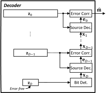
Figure 3: AIC decoder.

The decoder further performs error correction as follows:

$$\mathbf{x}_{D-1}=\mathbf{\bar{x}}_{D-1}\oplus\mathbf{e}_{D-1}$$ (34)

where the vector $\mathbf{\bar{x}}_{D-1}$ is computed using (19) by setting $i=D-1$.

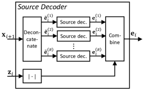
Figure 4: Source decoder. $|\cdot|$ denotes absolute value.

The above steps are repeated until the decoded information message ${\bf\hat{m}}$ is obtained by correcting the errors that corrupted the initial transmission as follows:

$${\bf\hat{m}}=\mathbf{\bar{x}}_{0}\oplus\mathbf{e}_{0}.$$ (35)

II-C Average Codeword Length

The AIC codeword is obtained as the concatenation of the information message $\mathbf{m}$ and the source-coded error location words $\mathbf{x}_{i},i=1,\ldots,D_{\rm MAX}$ in the following way:

$$\mathbf{X}=[\mathbf{m},\mathbf{x}_{1},\ldots,\mathbf{x}_{D_{\rm MAX}}].$$ (36)

The length of $\mathbf{X}$, denoted by $N$, is a RV whose expected value can be computed as follows:

$$E[N]=E\left[\sum_{i=0}^{D_{\rm MAX}}N_{i}\right]=\sum_{i=0}^{D_{\rm MAX}}E\left[N_{i}\right]$$ (37)

where $N_{0}$ is the message length, $N_{i},i=1,\ldots,D_{\rm MAX},$ is the length of the $i^{\rm th}$ source-coded error location vector and $D_{\rm MAX}$ is the maximum number of iterations. Thanks to source coding, each source-coded error location vector has shorter expected length compared to the length of the previous source-coded error location vectors, that is:

$$E[N_{i}\mid N_{i-1}]<N_{i-1}.$$ (38)

We prove (38) by noting that Huffman’s expected codeword length approaches the entropy rate of the source that produces its input sequence as $H$ approaches infinity. Thus, the source-coded error location vector length, denoted as $\ell(\mathbf{\tilde{e}}_{i}^{(r)})$, has the following expected value:

$$\lim_{H\to\infty}E[\ell(\mathbf{\tilde{e}}_{i}^{(r)})\mid\ell(\mathbf{e}_{i}^{(r)})]={\cal H}_{2}(\pi_{r})\ell(\mathbf{e}_{i}^{(r)})$$ (39)

where ${\cal H}_{2}(\pi_{r})\triangleq-\pi_{r}\log_{2}\pi_{r}-(1-\pi_{r})\log_{2}(1-\pi_{r})$ is the binary entropy function and $\pi_{r}$ is the probability that a given bit of $\mathbf{e}_{i}^{(r)}$ is ’1’. Thus, when $H$ approaches infinity, the expected length of the $i^{\rm th}$ source coded error location word $\mathbf{x}_{i}$ can be obtained as follows:

$$E[N_{i}\mid N_{i-1}] \stackrel{{\scriptstyle(a)}}{{=}} \sum_{r=0}^{R}{E[\ell(\mathbf{\tilde{e}}_{i-1}^{(r)})\mid N_{i-1}]}$$ (40)

$$\stackrel{{\scriptstyle(b)}}{{=}} \sum_{r=0}^{R}{{\cal H}_{2}(\pi_{r})E[\ell(\mathbf{e}_{i-1}^{(r)})\mid N_{i-1}]}$$ (41)

$$= \sum_{r=0}^{R}{{\cal H}_{2}(\pi_{r})\rho_{r}N_{i-1}}$$ (42)

$$= \alpha N_{i-1}$$ (43)

where, in the above chain of equations, (a) follows from the fact that $\mathbf{x}_{i}$ is obtained by concatenation of compressed error subvectors $\mathbf{\tilde{e}}_{i-1}^{(r)}$ and (b) follows from (39). Moreover, in (43) we defined

$$\alpha\triangleq\sum_{r=0}^{R}{{\cal H}_{2}(\pi_{r})\rho_{r}}.$$ (44)

Th prove (38), it must be shown that $\alpha<1$. This inequality follows straightforwardly from the facts that $\rho_{r}$ is a probability distribution, therefore $\sum_{r=0}^{R}\rho_{r}=1$, and the binary entropy is ${\cal H}_{2}(\pi_{r})\leq 1,\forall r=0,\ldots,R$.

By the law of total expectation, (43) yields

$$E[N_{i}] = \sum_{k\in\mathbb{N}}E[N_{i}\mid N_{i-1}=k]P(N_{i-1}=k)$$ (45)

$$= \sum_{k\in\mathbb{N}}\alpha kP(N_{i-1}=k)$$ (46)

$$= \alpha E[N_{i-1}]$$ (47)

$$= \alpha^{i}N_{0}$$ (48)

where $N_{0}=K$ is the message length. Eq. (48) shows that the expected lengths of the source-coded error location vectors are exponentially decreasing according to a geometric progression with common ratio $\alpha$. By combining (48) and (37) we finally obtain

$$E[N]=\frac{1-\alpha^{D_{\rm MAX}+1}}{1-\alpha}K.$$ (49)

The above derivations have been obtained in the limit of $H$ approaching $\infty$. With finite $H$, the Huffman encoder will produce codewords with larger average length, therefore the right-hand side (RHS) of (49) can be interpreted as a lower bound to the average codeword length. In the following section, we will use the RHS of (49) to derive an upper bound on the SE. We will show that the obtained upper bound is tight in many cases, thereby proving that (49) provides an accurate prediction of the average codeword length obtained using finite values of $H$ – predictions turn out to be accurate even for rather small values of $H$, e.g., $H<10$.

III Performance Evaluation

In this section, we show the results of AIC performance evaluation. In Subsec. III-A we evaluate the AIC SE and compare it with the SE achieved by conventional error correction codes through the Polyanskiy, Poor and Verdú (PPV) normal approximation [2]. The comparison shows that AIC performs better than any conventional error correction code. We also show that AIC performs better than the following feedback codes: a feedback code with fixed codeword length – Deepcode [10] – and a feedback code with variable codeword length – CEC [11]. In Subsec. III-B we evaluate the cumulative distributions of number of iterations and codeword length. We compare the codeword length distribution of AIC with the distribution produced by NR HARQ and conclude that AIC’s codeword length dispersion is more contained than the dispersion of codeword lengths produced by NR HARQ.

III-A Spectral Efficiency

The performance of AIC is evaluated in terms of SE vs. SNR of the received forward signal for given target BLER. The SE is defined as follows:

$${\rm SE}\triangleq\frac{KQ}{E[N]}(1-{\rm BLER})\;\rm[bits/s/Hz]$$ (50)

where $K$ is the message length and $Q$ is the modulation order. The BLER is defined as follows:

$${\rm BLER}\triangleq P(\hat{\mathbf{m}}\neq\mathbf{m}).$$ (51)

A simple analytical upper bound to the AIC spectral efficiency can be obtained by combining (49) and (50) with BLER = 0. The resulting equation is the following:

$$SE_{\rm UB}\triangleq\frac{(1-\alpha)Q}{1-\alpha^{D_{\rm MAX}+1}}.$$ (52)

In the rest of this section, the average codeword length $E[N]$ and BLER are evaluated by link-level simulation. The corresponding SE is computed using (50). For conventional codes, the evaluations are carried out at a given target BLER ($10^{-4}$). As for AIC, we let the encoder iterate until error-free transmission occurs, thereby producing BLER = 0. Such a comparison might be deemed unfair or inaccurate. However, according to our observations, there is no noticeable difference between the SE of error-free AIC and the SE of AIC with nonzero BLER as long as the BLER remains below $10^{-2}$. Based on the above observation, we conclude that the comparison between SE of error-free AIC and SE of conventional codes with BLER $=10^{-4}$ is accurate.

SNR [dB]	$\boldsymbol{\theta}^{*}$
-2	$(0,1.42,\infty)$
0	$(0,1.72,\infty)$
2	$(0,2.07,\infty)$
4	$(0,2.47,\infty)$
6	$(0,2.92,\infty)$

TABLE I: Quantization thresholds obtained for QPSK modulation and $R=2$.

The forward channel is impaired by Additive White Gaussian Noise (AWGN) and by Quasi-Static Rayleigh fading (QSRF). On the QSRF channel, each transmitted word ${\bf x}_{i},i=0,\ldots,D$, is subject to a corresponding fading coefficient $h_{i}$, as described by the following equation:

$$\mathbf{y}_{i}=h_{i}\mathbf{s}_{i}+{\boldsymbol{\nu}}_{i},\quad i=0,\ldots,D$$ (53)

where $h_{i},i=0,\ldots,D$, are statistically independent fading RVs drawn from a Rayleigh distribution with a suitably chosen mean so as to obtain unit average received signal energy. The vector ${\boldsymbol{\nu}}_{i}$ contains $N_{i}$ statistically independent complex Gaussian noise signals with zero mean and variance $\sigma_{\boldsymbol{\nu}}^{2}$. The SNR for the $i^{\rm th}$ transmission is defined as follows:

$${\rm SNR}_{i}\triangleq\frac{h_{i}^{2}}{\sigma_{\boldsymbol{\nu}}^{2}}.$$ (54)

The performance evaluation results on the QSRF channel are reported as BLER vs. average SNR, where the average SNR is defined as follows:

$$\overline{\mathrm{SNR}}=E[\mathrm{SNR}_{i}].$$ (55)

The LLRs quantization thresholds are determined as in (9), where the first threshold is set as ${\boldsymbol{\theta}}_{0}=0$. Table I shows the values of optimal quantization thresholds obtained with $R=2$ and SNRs between -2 dB and 6 dB. The simulation parameters used for performance evaluation are summarized in Table II.

Parameter	Value
Codeword length ($N$) [bits]	128
Modulation	QPSK, 16QAM, 64QAM
Modulation labeling	Gray
Number of quantization thresholds ($R$)	$1,\ldots,8$
Huffman dictionary size ($2^{H}$)	$2^{8}$
Maximum number of iterations ($D_{\rm MAX}$)	$\infty$
Target BLER	$10^{-4}$

TABLE II: Performance evaluation parameters.

Figure 5 shows the SE vs. SNR performance of AIC with QPSK modulation. The SE obtained with $R=1$ is shown as a solid red curve labeled ”AIC SE (R=1)”; the corresponding SE upper bound (52) is shown as a dashed red curve labeled ”AIC SE UB (R=1)”. The SE obtained with $R=2$ is shown as a solid purple curve labeled ”AIC SE (R=2)”; the corresponding SE upper bound (52) is shown as a dashed purple curve labeled ”AIC SE UB (R=2)”.

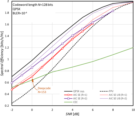
Figure 5: Spectral efficiency vs. SNR of QPSK-modulated AIC on AWGN. ”AIC SE” denotes AIC spectral efficiency obtained by Monte Carlo simulation. ”AIC SE UB” is the upper bound (52).

The plot of Figure 5 also shows the SE of the CEC method [11]. CEC has significantly smaller SE compared to AIC, especially at high SNR. The poor performance of CEC is mainly due to the Shannon-Fano source coding of CEC – Shannon-Fano performance with short codewords is worse than Huffman coding. The Polyanskiy, Poor and Verdú (PPV) normal approximation [2] is used to predict the performance that can be achieved by state-of-art conventional codes. To the best of the authors’ knowledge, there is no conventional short code that performs better than PPV, according to a summary of state-of-art short codes’ performance in [4]. It can be observed that AIC performs significantly better than PPV. Even with a single quantization threshold ($R=1$), AIC provides SNR gains larger than 1 dB in the range of SEs between 0.4 and 1 bits/s/Hz. AIC with $R=2$ provides even larger gains as its performance approaches the capacity of QPSK modulation up to within a small gap for SNRs below 2 dB. Values of $R>2$ do not provide significant gains compared to $R=2$. Compared to Deepcode [10], AIC with $R=2$ shows an SNR gain of about 1.6 dB. The upper bound (52) provides an accurate prediction of the real SE. For $R=1$, the gap between upper bound and real SE is smaller than $5.5\%$ for all the evaluated SNRs in Figure 5. For $R=2$, the gap between upper bound and real SE is between $5.8\%$ and $9.4\%$ in the evaluated range of SNRs. The reason for the higher inaccuracy observed with $R=2$ will be subject of investigation in future works.

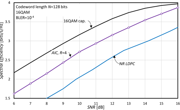
(a) 16QAM.

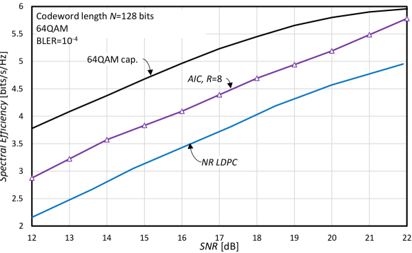
(b) 64QAM.

Figure 6: Spectral efficiency vs. SNR of AIC on AWGN.

Figure 6(a) and Figure 6(b) show the SE vs. SNR performance of AIC with 16QAM and 64QAM modulations. With 16QAM and 64QAM, a larger number of quantization thresholds is needed compared to QPSK, as each component of the QAM modulation signal uses more amplitude levels. It has been found by numerical evaluation that $R=4$ is close to optimal for 16QAM, while $R=8$ is close to optimal for 64QAM. As there is no available theoretical result similar to PPV for 16QAM and 64QAM, we compare the AIC performance with one of the best conventional channel codes known to-date – NR LDPC codes. The SNR gain of 16QAM/64QAM modulated AIC compared to the NR LDPC code with same modulations is larger than 2 dB, whereas the AIC SE is 0.5 bits/s/Hz larger than the SE of NR LDPC codes on the whole range of SNRs that we evaluated. These results show that AIC achieves arbitrarily high spectral efficiencies by using conventional high-order modulations and provides remarkable gains compared to conventional codes.

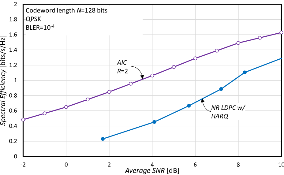
Figure 7: Spectral efficiency of AIC with QPSK modulation on quasi-static Rayleigh fading channel.

Figure 7 shows the spectral efficiency of AIC with QPSK modulation on the QSRF channel described by (53). The AIC SE is compared with the SE of the NR LDPC code with QPSK modulation and Hybrid Automatic Repeat reQuest (HARQ) [12, 3]. The reason for considering HARQ in the QSRF performance evaluation of LDPC codes is that quasi-static fading combines detrimentally with the channel dispersion [2], that characterizes the AWGN channel when used for transmission of short codewords, so as to make reliable communication practically impossible at any reasonable SNR. HARQ counteracts quasi-static fading by adaptively decreasing the code rate based on the channel fading realization. According to the evaluations shown in Figure 7, AIC shows a large SNR gain compared to NR LDPC codes with HARQ – more than 4 dB for SE between 0.4 and 1.2 bits/s/Hz.

III-B Distribution of Number of Iterations and Codeword Length

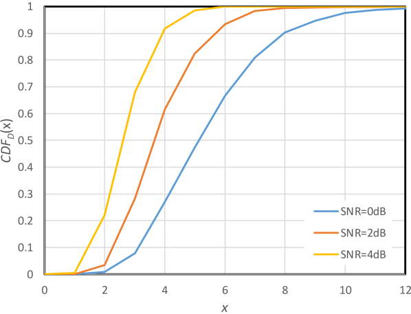
(a) CDF of number of iterations (56).

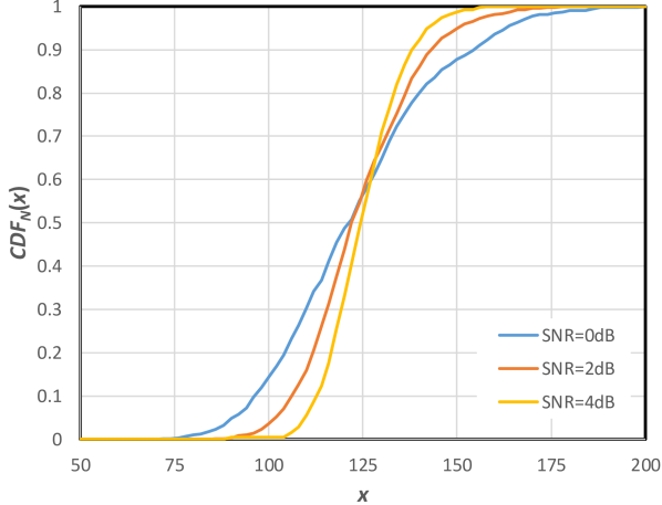
(b) CDF of codeword length (60).

Figure 8: Cumulative Distrbution Functions (CDFs) of (a) number of iterations $D$ and (b) codeword length $N$.

The AIC encoding procedure performs a variable number of iterations and produces codewords of variable length – number of iterations and the codeword lengths are unpredictable as they ultimately depend on the forward channel noise and fading realizations.

Uncertainty on the number of iterations results in unpredictable transmission delays – a challenging situation for higher-layer protocols and for delay-sensitive applications. In order to provide an assessment of AIC in terms of number of iterations, we evaluate empirically the Cumulative Distribution Function (CDF) of the number of iterations, which is defined as follows:

$$CDF_{D}(x)=P(D\leq x)$$ (56)

Figure 8(a) shows $CDF_{D}(x)$ for QPSK-modulated AIC on AWGN channel with SNR=0 dB, 2 dB, and 4 dB. The CDF curves are obtained by simulation with 1000 codewords. It can be observed that for SNR=0 dB (blue curve), the number of iterations needed to complete a message transmission takes values between 2 and 13, where the average number of iterations is approx. 5. With higher SNR, the number of iterations is significantly smaller – 1 to 5 iterations for SNR=4 dB (yellow curve), where the average number of iterations is approximately 2.5.

The number of iterations has a significant impact on the transmission latency. A contained number of iterations produces shorter transmissions, thereby making the method suitable for low-latency applications. AIC is a promising candidate for low-latency applications thanks to its contained average number of iterations. However, AIC cannot guarantee that all transmissions will be successfully completed in any given number of iterations. A simple workaround to deal with the above issue consists in stopping the transmission after a maximum number of iterations $D_{\rm MAX}$, regardless of whether there are remaining errors. If there are remaining errors in the last iteration, the message transmission fails, thereby producing BLER $>0$. The relationship between BLER and $D_{\rm MAX}$ is captured by the function $CDF_{D}(x)$ of (56): for a given $D_{\rm MAX}$, $CDF_{D}(D_{\rm MAX})$ is the ratio of message transmissions that require $D_{\rm MAX}$ or less iterations. Therefore, for a given $D_{\rm MAX}$, BLER can be obtained as follows:

$$BLER=1-{CDF}_{D}(D_{\rm MAX})$$ (57)

It follows that, for a given target block error rate ${BLER}_{\rm T}$, the maximum number of iterations needed to achieve that BLER is the following:

$$D_{\rm MAX}=\min\{x\in\mathbb{N}:{CDF}_{D}(x)\geq 1-{BLER}_{\rm T}\}$$ (58)

or equivalently:

$$D_{\rm MAX}=\lceil{CDF}_{D}^{-1}(1-{BLER}_{\rm T})\rceil$$ (59)

where ${CDF}_{D}^{-1}$ denotes the inverse function of ${CDF}_{D}$. Eq. (59) can be combined into (49) and (52) so as to provide expressions that capture the interplay between target BLER, average codeword length and spectral efficiency.

Similar as the uncertainty on the number of iterations, the uncertainty on the codeword length might be an issue for transceiver design as the sizes of transmitter/receiver buffers involved in encoding and decoding would have to be determined based on worst-case situations. In order to provide an assessment of AIC in terms of codeword lengths, we evaluate by simulation the codeword length CDF as follows:

$${CDF}_{N}(x)=P(N\leq x).$$ (60)

Figure 8(b) shows a plot of ${CDF}_{N}(x)$ obtained by simulation with 1000 codewords. For SNR = 0 dB (blue curve), the codeword length $N$ takes values in a range between 72 bits and 206 bits. As the SNR increases, the range shrinks – for SNR = 4dB (yellow curve), $N$ is distributed between 90 bits and 164 bits. In Table III, the above values are summarized and a codeword length dispersion value is computed as $N_{\rm max}/N_{\rm min}$ in the rightmost column. For comparison, NR HARQ is typically configured to perform up to four transmissions, thereby producing codewords whose length is up to four times the length of the initial transmission, thus $N_{\rm max}/N_{\rm min}=4$. Thus, the HARQ codeword lengths are typically spread over larger intervals compared to AIC.

SNR	$K$	$N_{\rm min}$	$N_{\rm max}$	$N_{\rm max}/N_{\rm min}$	$N_{\rm max}/N_{\rm min}$
[dB]	[bits]	[bits]	[bits]	(AIC)	(NR HARQ)
0	54	72	206	2.86	4
2	72	86	186	2.16	4
4	90	90	164	1.82	4

TABLE III: Dispersion of codeword length $N$.

It can be concluded that AIC’s number of iterations and codeword length, although being unpredictable, take values in rather contained intervals, thereby not posing significant challenges to transceiver design or delay-sensitive applications.

IV Conclusion

A new error correction code for channels with feedback – the Accumulative Iterative Code – has been described in this paper. AIC encoder and decoder interact with each other by exchanging signals through the forward and feedback channels. The AIC encoder continues to perform iterations until an error-free forward transmission occurs.

The new code achieves spectral efficiency close to channel capacity in a wide range of SNRs even for transmission of short information messages – a situation where conventional ECC show a rather large gap between SE and channel capacity. In the same time, AIC provides arbitrarily low error rates, thereby being suitable for applications demanding extremely high reliability. Performance evaluations on the AWGN channel and quasi-static Rayleigh fading show that AIC provides significant spectral efficiency and SNR gains compared to conventional ECC methods.

Finally, it has been shown that the number of encoding iterations is fairly small. The codeword length, although unpredictable, takes values in a contained interval, thereby not posing significant challenges to transceiver design.

Appendix A

In Section II-A, it has been shown that (24) holds with equality for BPSK and Gray-mapped QPSK modulations. We also claimed that (24) holds with the “$\cong$” sign for higher-order modulations within their typical operating SNR ranges. Here, we prove by numerical evaluations that the above statement is true.

Eq. (24) combined with (28) and (29) yields:

$$p_{0,-r}(\boldsymbol{\theta})\cong p_{1,r}(\boldsymbol{\theta}).$$ (61)

In order to prove (61), we define a quadratic dispersion – similar as the probabilistic concept of variance – for the probabilities $p_{0,-r}(\boldsymbol{\theta})$ and $p_{1,r}(\boldsymbol{\theta})$ as follows:

$$\delta_{r}\triangleq(p_{0,-r}(\boldsymbol{\theta})-E_{r})^{2}+(p_{1,r}(\boldsymbol{\theta})-E_{r})^{2}$$ (62)

where $E_{r}$ is the average of $p_{0,-r}(\boldsymbol{\theta})$ and $p_{1,r}(\boldsymbol{\theta})$, and then we determine the maximum dispersion as follows:

$$\Delta=\max_{r=0,\ldots,R}{\delta_{r}}$$ (63)

The values of maximum dispersion obtained for 16QAM and 64QAM within their typical SNR ranges are shown in Table IV. It can be seen that the dispersion $\Delta$ remains very contained for all SNR values. We conclude that (24) holds for 16QAM and 64QAM within their typical SNR ranges of operation.

SNR [dB]	16QAM	64QAM
6	5.72e-6	–
8	4.55e-8	–
10	1.60e-8	–
12	9.09e-10	4.93e-7
14	1.22e-9	1.13e-8
16	7.74e-10	2.08e-9
18	–	1.57e-9
20	–	1.06e-9
22	–	8.73e-11

TABLE IV: Maximum dispersion $\Delta$ for 16QAM and 64QAM.

References

- [1] Third Generation Partnership Project, “Technical Specification Group Services and System Aspects; Study on Communication for Automation in Vertical Domains (Release 16).” 3GPP TR 22.804 V16.2.0, Dec 2018.
- [2] Y. Polyanskiy, H. V. Poor, and S. Verdú, “Channel coding rate in the finite block length regime,” IEEE Transactions on Information Theory, vol. 56, no. 5, pp. 2307–2359, May 2010.
- [3] Third Generation Partnership Project; Technical Specification Group Radio Access Network; NR, “Multiplexing and channel coding (Release 15),” 3GPP TS 38.212 V15.4.0, Dec 2018.
- [4] M. Shirvanimoghaddam, M. S. Mohammadi, R. Abbas, A. Minja, C. Yue, B. Matuz, G. Han, Z. Lin, W. Liu, Y. Li, S. Johnson, and B. Vucetic, “Short block-length codes for ultra-reliable low latency communications,” IEEE Communications Magazine, vol. 57, no. 2, pp. 130–137, February 2019.
- [5] T. M. Cover and J. A. Thomas, Elements of Information Theory, ed. John Wiley & Sons, 2006.
- [6] J. Schalkwijk and T. Kailath, “A coding scheme for additive noise channels with feedback–i: No bandwidth constraint,” IEEE Transactions on Information Theory, vol. 12, no. 2, pp. 172–182, 1966.
- [7] A. Ben-Yishai and O. Shayevitz, “Interactive schemes for the AWGN channel with noisy feedback,” IEEE Transactions on Information Theory, vol. 63, no. 4, pp. 2409–2427, 2017.
- [8] J. G. Proakis and M. Salehi, Digital communications, ed. McGraw-Hill, 2008.
- [9] A. El Gamal and Y.-H. Kim, Network Information Theory. Cambridge, UK: Cambridge University Press, 2011.
- [10] H. Kim, Y. Jiang, S. Kannan, S. Oh, and P. Viswanath, “Deepcode: Feedback codes via deep learning,” IEEE Journal on Selected Areas in Information Theory, pp. 1–1, 2020.
- [11] J. M. Ooi and G. W. Wornell, “Fast iterative coding techniques for feedback channels,” IEEE Transactions on Information Theory, vol. 44, no. 7, pp. 2960–2976, 1998.
- [12] S. Lin and D. J. Costello, Error Control Coding. Prentice-Hall, 1983.