An adaptive high-order surface finite element method for polymeric self-consistent field theory on general curved surfaces

Abstract

In this paper, we develop an adaptive high-order surface finite element method (FEM) incorporating spectral deferred correction method for chain contour discretization to solve polymeric self-consistent field equations on general curved surfaces. The high-order surface FEM is obtained by the high-order surface geometrical approximation and the high-order function space approximation. Numerical results demonstrate that the precision order of these methods is consistent with theoretical prediction. In order to describe the sharp interface in the strongly segregated system more accurately, an adaptive FEM equipped with a new Log marking strategy is proposed. Compared with the traditional strategy, the Log marking strategy can not only label the elements that need to be refined or coarsened, but also give the refined or coarsened times, which can make full use of the information of a posterior error estimator and improve the efficiency of the adaptive algorithm. To demonstrate the power of our approach, we investigate the self-assembled patterns of diblock copolymers on several distinct curved surfaces. Numerical results illustrate the efficiency of the proposed method, especially for strongly segregated systems with economical discretization nodes.

1 Introduction

In recent years, microphase separation of block copolymers under various types of geometrical confinements (including Euclidean and manifold confinements) has attracted tremendous attention due to their industrial applications [1, 2]. Geometric constraints drastically affect the formation of ordered structures under which some traditional ordered phases of block copolymers are rearranged to form novel patterns [1, 2, 3, 4, 5, 6]. Theories play an important role in understanding and predicting the phase behavior of block copolymers under geometrical confinements [7, 8, 9, 10, 11]. Among these theories, self-consistent field theory (SCFT) [11] is one of the most powerful tools in studying the self-assembly behaviors of inhomogeneous polymers and related soft-matter systems.

There have been a few studies done on the surface SCFT calculations, versus numerous works on computing bulk structures based on SCFT. Chantawansri et al. [9] and Vorselaars et al. [12] used the spherical harmonic method to numerically simulate the SCFT model confined on the spherical surface and in the spherical shell, respectively. The global spherical harmonic method has spectral accuracy, however, it can not extend to general curved surfaces. For computing the SCFT model on general surface, Li et al. [8, 13] proposed a method similar to the finite volume method. However, there has been no theory (numerical result) to guarantee (rigorously demonstrate) the computational precision. Besides that, Li’s method can not be applied to strongly segregated systems when interaction parameter $\chi N>25$ for diblock copolymer melt. Meanwhile, even for relatively weak interaction systems $\chi N<25$, Li’s method still requires a large number contour discretization points (more than $1000$) to reduce the free-energy discrepancy about $5\times 10^{-5}$. Precisely computing strongly segregated systems is still a challenge in the SCFT computation, especially for general surface confinement. In this work, we are devoted to developing efficient high-order numerical methods for polymer SCFT on general curved surfaces.

In the past several decades, many numerical approaches have been developed to address surface problems, including the level-set method [16], the close point method [15], and the surface FEM [17, 18, 23, 24]. In this paper, we focus on the surface FEM. Dziuk [17] firstly proposed a linear FEM to solve the Laplace-Beltrami equation on arbitrary surfaces. Demlow and Dziuk [18] presented an adaptive linear surface FEM, and then Demlow [19] generalized the surface FEM theory to a high-order case. Wei et al.[21] generalized the superconvergence results and several gradient recovery approaches of linear FEM from flat spaces to general curved surfaces for the Laplace-Beltrami equation with mildly structured triangular meshes. Bonito and Demlow [22] gave the new posteriori error estimates with sharper geometric error estimators for surface FEMs. After about 25 years of development, the surface FEM has been applied to a wide range of scientific problems, see recent review papers [23, 24] and references therein.

In our previous work [10], we proposed a linear surface FEM to study the microphase separation of block copolymers on general curved surfaces. However, in SCFT calculations, using the linear surface FEM to achieve a relatively high numerical precision may result in heavy computational complexity. Meanwhile, in strong segregation regime, self-assembled structures have two-scale spatial distribution: sharp interfaces and damped internal densities, making the uniform mesh method inefficient. Therefore it is necessary to improve this numerical method. The main contributions of this work include:

• We present an adaptive high-order surface FEM for polymeric SCFT. It is high order both in space (surface discretization and function space approximation) and in time through incorporating spectral deferred correction method for chain contour integration. A concrete way to construct arbitrary order surface FEM is also given.

• We propose a novel and efficient marking strategy in the adaptive method. This new marking approach does not only denote which mesh element needs to be changed, but also provides the times of refinement or coarseness. Compared with existing marking strategies, the new approach can efficiently make full use of the information of a posterior error estimator.

• Our developed method is attractive for strongly segregated systems. Numerical results for strongly segregated systems demonstrate that our proposed approach can achieve the prescribed precision with an economical computational cost both in space and time directions.

The rest of this paper is organized as follows. In Sec. 2, we introduce a self-consistent field model on general curved surfaces of diblock copolymer melt as an example to demonstrate our method. In Sec. 3, we present the concrete construction procedure of adaptive high-order surface FEM in detail and apply it to solve the propagator equation. In Sec. 4, we incorporate the spectral deferred correction scheme for the contour discretization into the adaptive high-order FEM. In Sec. 5, we examine the efficiency of the proposed methods through sufficient numerical examples. It should be noted that the proposed method is also suitable for other polymeric systems.

2 Surface self-consistent field theory

In this section, we present the SCFT for an incompressible AB diblock copolymer melt on a generally curved surface using the standard Gaussian chain model. We consider $n$ AB diblock copolymers confined on a curved surface $\mathcal{M}$ whose measure is $|\mathcal{M}|$. The volume fraction of A block is $f$ and that of B block is $1-f$, the total degree of polymerization of a diblock copolymer is $N$. The field-based Hamiltonian for the incompressible diblock copolymer melt is [11]

$$H=\frac{1}{|\mathcal{M}|}\int_{\mathcal{M}}\left\{-\omega_{+}(\bm{x})+\frac{\omega_{-}^{2}(\bm{x})}{\chi N}\right\}\mathrm{d}\bm{x}-\log Q[\omega_{+}(\bm{x}),\omega_{-}(\bm{x})],$$ (1)

where $\chi$ is the Flory-Huggins parameter to measure the interaction between segments A and B. The term $\omega_{+}(\bm{x})$ is the fluctuating pressure field, and $\omega_{-}(\bm{x})$ is the exchange chemical potential field. The pressure field enforces the local incompressibility, while the exchange chemical potential field is conjugate to the density operators. $Q$ is the single chain partition function.

First-order variations of the Hamiltonian with respect to the fields $\omega_{\pm}(\bm{x})$ lead to the following mean-filed equations,

$$\frac{\delta H}{\delta\omega_{+}(\bm{x})} =\varphi_{A}(\bm{x})+\varphi_{B}(\bm{x})-1=0,$$ (2)

$$\frac{\delta H}{\delta\omega_{-}(\bm{x})} =\frac{2\omega_{-}(\bm{x})}{\chi N}-[\varphi_{A}(\bm{x})-\varphi_{B}(\bm{x})]=0.$$ (3)

$\varphi_{A}(\bm{x})$ and $\varphi_{B}(\bm{x})$ are the monomer densities of blocks A and B, respectively.

$$\varphi_{A}(\bm{x})=\frac{1}{Q}\int_{0}^{f}q(\bm{x},t)q^{\dagger}(\bm{x},t)\,\mathrm{d}t,$$ (4)

$$\varphi_{B}(\bm{x})=\frac{1}{Q}\int_{f}^{1}q(\bm{x},t)q^{\dagger}(\bm{x},t)\,\mathrm{d}t.$$ (5)

The single chain partition function $Q$ can be calculated by

$$Q=\frac{1}{|\mathcal{M}|}\int_{\mathcal{M}}q(\bm{x},1)\,\mathrm{d}\bm{x}.$$ (6)

The forward propagator $q(\bm{x},t)$ denotes the probability distribution of the chain in contour node $t$ at surface position $\bm{x}$. The variable $t$ is used to parameterize each copolymer chain such that $t=0$ represents the tail of the A block and $t=f$ is the junction between the A and B blocks, $t=1$ is the end of the B block. From the continuous Gaussian chain model [25], $q(\bm{x},t)$ satisfies the PDE

$$\frac{\partial}{\partial t}q(\bm{x},t) =[\Delta_{\mathcal{M}}-w(\bm{x},t)]q(\bm{x},t),$$ (7)

$$q(\bm{x},0) =1,$$

$$w(\bm{x},t) =\left\{\begin{array}[]{rl}\omega_{+}(\bm{x})-\omega_{-}(\bm{x}),&0\leq t\leq f,\\ \omega_{+}(\bm{x})+\omega_{-}(\bm{x}),&f\leq t\leq 1.\end{array}\right.$$

$\Delta_{\mathcal{M}}$ is the Laplace-Beltrami operator which reads as follows

$$\Delta_{\mathcal{M}}v=div_{\mathcal{M}}\cdot(\nabla_{\mathcal{M}}v),$$

where $\mathcal{M}$ is a two-dimensional, compact, and $\mathcal{C}^{2}$-hypersurface in $\mathbb{R}^{3}$. $\nabla_{\mathcal{M}}$ and $div_{\mathcal{M}}$ are the tangential gradient and divergence operators, respectively, their definitions can be found in [17, 18]. The Sobolev space on surface $\mathcal{M}$ is

$$H^{p}(\mathcal{M})=\{v\in L^{2}(\mathcal{M})\ |\ D^{\alpha}v\in L^{2}(\mathcal{M}),\ |\alpha|\leq p\}.$$

The backward propagator $q^{\dagger}(\bm{x},t)$ represents the probability distribution from $t=1$ to $t=0$ satisfying

$$\frac{\partial}{\partial t}q^{\dagger}(\bm{x},t) =[\Delta_{\mathcal{M}}-w^{\dagger}(\bm{x},t)]q^{\dagger}(\bm{x},t),$$ (8)

$$q^{\dagger}(\bm{x},0) =1,$$

$$w^{\dagger}(\bm{x},t) =\left\{\begin{array}[]{rl}\omega_{+}(\bm{x})+\omega_{-}(\bm{x}),&0\leq t\leq 1-f,\\ \omega_{+}(\bm{x})-\omega_{-}(\bm{x}),&1-f\leq t\leq 1.\end{array}\right.$$

For closed surfaces, no boundary condition is needed. While for open surfaces, Eqns. (7) and (8) require boundary conditions to be well-posed. In this work, we use the homogeneous Neumann boundary condition for open surfaces. Certainly, other appropriate boundary conditions can be considered in the following proposed algorithm framework.

Finding equilibrium states of SCFT corresponds to solutions of Euler-Lagrange equation $\delta H/\delta\omega_{\pm}(\bm{x})=0$. Note that field functions $\omega_{\pm}(\bm{x})$ are related to the density functions $\varphi_{A}(\bm{x})$, $\varphi_{B}(\bm{x})$ which satisfy integral equations (4) and (5). The integrands in Eqns. (4) and (5) are related to PDEs (7) and (8). Thus it is a nonlocal problem. Usually, iteration methods are designed to update field functions $\omega_{\pm}(\bm{x})$. The standard SCFT iteration procedure is shown in the Fig. 1.

Figure 1: Flowchart of SCFT iteration.

It is important to note that the iteration approach for updating the fields $\omega_{+}(\bm{x})$ and $\omega_{-}(\bm{x})$ could be determined by the SCFT mathematical properties. The Hamiltonian $H$ of AB diblock copolymers can reach its local minima along the exchange chemical field $\omega_{-}(\bm{x})$ and achieve the maxima along the pressure field $\omega_{+}(\bm{x})$ [11]. For multicomponent polymer systems, an extended analysis of the SCFT model can be found in Ref. [26]. Several iteration methods have been proposed to find the saddle point, such as the semi-implicit Seidel method [27], which is based on the asymptotic expansion and global Fourier transformation. Similarly, the semi-implicit scheme using global spherical harmonic transformation can be extended to the spherical surface problems [9]. However, it may be impossible to obtain a global basis on general curved surfaces. Correspondingly, the semi-implicit scheme could not be obtained. Thus, we choose the alternative direction explicit Euler method to update fields, i.e.,

$$\omega_{+}^{k+1}(\bm{x}) =\omega_{+}^{k}(\bm{x})+\lambda_{+}[\varphi_{A}^{k}(\bm{x})+\varphi_{B}^{k}(\bm{x})-1],$$ (9)

$$\omega_{-}^{k+1}(\bm{x}) =\omega_{-}^{k}(\bm{x})-\lambda_{-}\left(\frac{2\omega_{-}^{k}(\bm{x})}{\chi N}-[\varphi^{k}_{A}(\bm{x})-\varphi^{k}_{B}(\bm{x})]\right),$$

where $\lambda_{\pm}$ are the iteration step size.

3 Adaptive high-order surface FEM

For the strongly segregated polymer systems, the self-assembled patterns have sharp interfaces and gradually changed internal structures. A uniform mesh method gives rise to a large amount of computational complexity. This section presents an adaptive high-order surface FEM to solve the propagators on general curved surfaces, obtaining better accuracy results with lower computation cost.

Consider a curved surface $\mathcal{M}$ with boundary $\mathcal{M}_{g}$ on which (7) and (8) are well-defined. Let $\mathcal{V}=H^{1}(\mathcal{M})$ be the trial and test function spaces. The variational formulation is stated as follows: find $q\in\mathcal{V}$ such that for $\forall v\in\mathcal{V}$

$$\left(\frac{\partial}{\partial t}q,v\right)_{\mathcal{M}}=-(\nabla_{\mathcal{M}}q,\nabla_{\mathcal{M}}v)_{\mathcal{M}}-(wq,v)_{\mathcal{M}},~{}~{}\text{ for all }~{}v\in\mathcal{V},$$ (10)

where $(\cdot,\cdot)_{\mathcal{M}}$ represents the $L^{2}$ inner product on curved surface $\mathcal{M}$.

3.1 The construction of high-order surface FEM space

Next we present the construction of the high-order surface FEM space. We first introduce the multi-index vector $\bm{m}:=(m_{0},m_{1},m_{2})$ with

$$m_{i}\geq 0,~{}i=0,1,2,\text{ and }\sum_{i=0}^{2}m_{i}=p.$$

The number of all possible of $\bm{m}$ is

$$n_{p}:=\begin{pmatrix}p+2\\ 2\end{pmatrix}.$$

Let $\alpha$ be a one-dimensional index starting from 0 to $n_{p}-1$ of $\bm{m}$, see Tab. 1 for the numbering rule.

Table 1: The numbering rule of multi-index $\bm{m}_{\alpha}$.

$\alpha$	$\bm{m}_{\alpha}$
$0$	$p$	$0$	$0$
$1$	$p-1$	$1$	$0$
$2$	$p-1$	$0$	$1$
$3$	$p-2$	$2$	$0$
$4$	$p-2$	$1$	$1$
$\vdots$	$\vdots$	$\vdots$	$\vdots$
$n_{p}-1$	$0$	$0$	$p$

For each multi-index $\bm{m}_{\alpha}=(m_{0},m_{1},m_{2})$, one can define a point $\bm{u}_{\alpha}=(\xi,\eta)=(m_{1}/p,m_{2}/p)$ on the reference triangle $\hat{\tau}$ (an isosceles right triangle with the right side length of $1$), and the corresponding barycentric coordinate $\bm{\lambda}=(\lambda_{0},\lambda_{1},\lambda_{2})$, where

$$\lambda_{0}=\frac{m_{0}}{p}=1-\xi-\eta,\quad\lambda_{1}=\frac{m_{1}}{p}=\xi,\quad\lambda_{2}=\frac{m_{2}}{p}=\eta.$$ (11)

Using the numbering rule, the spatial sorting of $\bm{u}_{\alpha}$ on $\hat{\tau}$ follows the rules shown in Fig. 2.

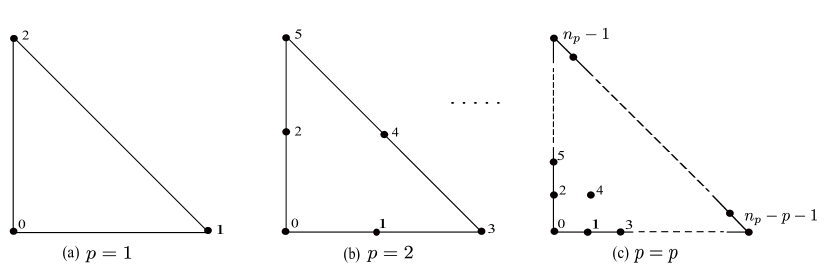
Figure 2: The spatial sorting rules for the points $\bm{u}_{\alpha}$ on the reference triangle $\hat{\tau}$.

Then for each multi-index $\bm{m}_{\alpha}$, one can construct the shape function of degree $p$ on the reference triangle $\hat{\tau}$ as follows

$$\phi_{\alpha}(\bm{u})=\frac{1}{\bm{m}_{\alpha}!}\prod_{i=0}^{2}\prod_{j=0}^{m_{i}-1}(p\lambda_{i}-j),$$ (12)

with

$$\bm{m}_{\alpha}!=m_{0}!m_{1}!m_{2}!\,,~{}~{}\text{ and }\prod_{j=0}^{-1}(p\lambda_{i}-j)=1,\quad i=0,1,2.$$

It is easy to verify that the shape function $\phi_{\alpha}$ defined above satisfies the interpolation property

$$\phi_{\alpha}(\bm{u}_{\beta})=\begin{cases}1,&\alpha=\beta,\\ 0,&\alpha\neq\beta,\end{cases}\quad\text{ with }\alpha,\beta=0,1,\cdots,n_{p}-1.$$ (13)

Obviously, $\{\phi_{\alpha}\}_{\alpha=0}^{n_{p}-1}$ are linearly independent. Notice that a formula similar to (12) can be found in [28]. Here we write it in a slightly different form and clearly show out its coefficients. Obviously, this formula can be easily extended to any dimensional geometric simplex and one can find such implementation in FEALPy [40].

Let $\mathcal{M}_{h}^{p}=\{\tau_{h}^{p}\}$ be a union of a set of triangle surfaces which is a continuous piecewise polynomial approximation of degree $p$ of surface $\mathcal{M}$. Each triangle surface $\tau_{h}^{p}$ is uniquely determined by a set of interpolation points $\{\bm{x}_{\alpha}\}_{\alpha=0}^{n_{p}-1}\subset\mathcal{M}$, which follows the same numbering rule as $\{\bm{u}_{\alpha}\}_{\alpha=0}^{n_{p}-1}$ on reference element $\hat{\tau}$, see Fig 3 for the case of $p=2$.

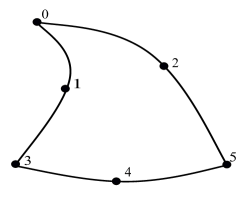
Figure 3: The quadric triangle surface $\tau^{2}_{h}$.

Then we can give a one-to-one mapping $\bm{x}:\hat{\tau}\mapsto\tau_{h}^{p}$ as follows

$$\bm{x}(\bm{u})=\sum_{\alpha=0}^{n_{p}-1}\bm{x}_{\alpha}\phi_{\alpha}(\bm{u}),\,\forall\bm{u}\in\hat{\tau},$$

and obviously,

$$\bm{x}_{\alpha}=\bm{x}(\bm{u}_{\alpha}),\alpha=0,1,\cdots,n_{p}-1.$$

In Fig. 4, we present a piecewise linear approximation surface $\mathcal{M}_{h}^{1}$ and a piecewise quadric surface $\mathcal{M}_{h}^{2}$ of a sphere.

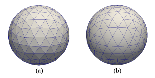
Figure 4: The piecewise linear surface $\mathcal{M}_{h}^{1}$ (a) and quadric surface $\mathcal{M}_{h}^{2}$ (b) triangular mesh on a sphere.

By the one-to-one mapping $\bm{x}:\hat{\tau}\mapsto\tau_{h}^{p}$, we can define the local basis function on $\tau_{h}^{p}$

$$\varphi_{\alpha}(\bm{x}):=\phi_{\alpha}(\bm{u}),\quad\forall\bm{x}(\bm{u})\in\tau_{h}^{p}\text{ with }\bm{u}\in\hat{\tau}.$$

Similarly, $\varphi_{\alpha}$ satisfies the interpolation property on interpolation points $\{\bm{x}_{\alpha}\}_{\alpha=0}^{n_{p}-1}$ of $\tau_{h}^{p}$

$$\varphi_{\alpha}(\bm{x}_{\beta})=\begin{cases}1,&\alpha=\beta,\\ 0,&\alpha\neq\beta,\end{cases}\quad\text{ with }\alpha,\beta=0,1,\cdots,n_{p}-1.$$

Furthermore, we know that the adjacent elements on high-order surface $\mathcal{M}_{h}^{p}$ will reuse the interpolation points on their shared nodes or edges. Suppose $\mathcal{M}_{h}^{p}$ has $NN$ nodes, $NE$ edges and $NC$ elements, the number of interpolation points on $\mathcal{M}_{h}^{p}$ is

$$N_{DoF}:=NN+(p-1)NE+\frac{(p-1)(p-2)}{2}NC.$$

For each interpolation point, one can construct a continuous piecewise global basis function on $\mathcal{M}_{h}^{p}$, which take value 1 at this interpolation point and 0 at others. On the element the interpolation point is located, the global basis function is exactly the local basis function corresponding to the interpolation point on that element. For simplicity, we still use $\varphi_{i}$ to represent the $i$-th global basis function.

Finally, we introduce a continuous piecewise polynomial space of degree $p$ defined on $\mathcal{M}_{h}^{p}$

$$\mathcal{V}_{h}^{p}:=\text{span}\{\varphi_{i}\}_{i=0}^{N_{DoF}-1}.$$

Notice that, the above definition is equivalent to the definition in the literature [23](Page 315, Intermediate remark).

The error of the surface FEM contains two parts: the geometric error arising from the approximation of $\mathcal{M}$ by the $\mathcal{M}^{p}_{h}$ and the function space approximation error coming from the approximation of an infinite-dimensional function space by a finite-dimensional space. As Demlow analyzed [19, 20], when employing finite element space of degree $p$ on the polynomial surface approximation of degree $k$, one can have

$$\|q-q^{l}_{h}\|_{L^{2}(\mathcal{M})}\leq Ch^{p+1}\|q\|_{H^{p+1}(\mathcal{M})}+Ch^{k+1}\|q\|_{H^{1}(\mathcal{M})},$$ (14)

where $q$ is the exact solution, $q^{l}_{h}$ denotes the lift of numerical solution $q_{h}$ from $\mathcal{M}^{p}_{h}$ to $\mathcal{M}$, $C$ depends on geometric properties of $\mathcal{M}$. In this work, we set $p=k$ to ensure that the approximation errors of the geometric and function space have the same accuracy.

3.2 Surface FEM discretization

By the finite-dimensional surface FEM space $\mathcal{V}_{h}^{p}$, the descrete weak formulation of (10) is: find

$$q_{h}(\bm{x},t)=\sum_{i=0}^{N_{DoF}-1}q_{i}(t)\varphi_{i}(\bm{x})\in\mathcal{V}_{h}^{p}$$

such that

$$\left(\frac{\partial}{\partial t}q_{h},v_{h}\right)_{\mathcal{M}_{h}^{p}}=-(\nabla_{\mathcal{M}_{h}^{p}}q_{h},\nabla_{\mathcal{M}_{h}^{p}}v_{h})_{\mathcal{M}_{h}^{p}}-(\omega_{h}q_{h},v_{h})_{\mathcal{M}_{h}^{p}},~{}~{}\text{ for all }v_{h}\in\mathcal{V}_{h}^{p}.$$ (15)

Let $v_{h}=\varphi_{j}$, $j=0,1,\cdots,N_{DoF}-1$, we have the matrix form of (15)

$$\bm{M}\frac{\partial}{\partial t}\bm{q}(t)=-(\bm{A}+\bm{F})\bm{q}(t),\\$$ (16)

where

$$\bm{q}(t)=\left(q_{0}(t),q_{1}(t),\cdots,q_{N_{DoF}-1}(t)\right)^{T},$$

and

$$\bm{M}_{i,j}=(\varphi_{i},\varphi_{j}),\quad\bm{A}_{i,j}=(\nabla_{\mathcal{M}_{h}^{p}}\varphi_{i},\nabla_{\mathcal{M}_{h}^{p}}\varphi_{j}),\quad\bm{F}_{i,j}=(\omega_{h}\varphi_{i},\varphi_{j}).$$

3.3 Adaptive surface FEM

In this subsection, we present the adaptive mesh method to obtain a high-precision numerical solution with less computational complexity. The adaptive method can automatically rearrange mesh grids according to the error distribution over each mesh element. The adaptive procedure used in the SCFT calculation contains

Step 1

Solve the SCFT model and obtain the numerical solution on a given mesh.

Step 2

Calculate a posterior error estimator on each element from current numerical results.

Step 3

Mark mesh elements according to the error estimator.

Step 4

Refine or coarsen the marked elements to update the mesh.

Step 5

Go to Step 1 until the desired error is satisfied.

Define the error estimator of the indicator function $u_{h}$ on each element $\tau$ as $e_{\tau}$,

$$e_{\tau}=\|G_{h}u_{h}\|_{\tau},$$ (17)

where $\|\cdot\|_{\tau}$ is denoted as the $L^{2}$ norm on $\tau$. $G_{h}u_{h}$ is the harmonic average operator [29]

$$G_{h}u_{h}(\bm{x}_{i}):=\frac{1}{\sum_{j=1}^{n}1/|\tau_{j}|}\sum_{j=1}^{n}\frac{1}{|\tau_{j}|}\nabla_{\mathcal{M}_{h}^{p}}u_{h}\Big{|}_{\tau_{j}}(\bm{x}_{i}).$$ (18)

$n$ is the number of elements $\tau_{j}$ with $\bm{x}_{i}$ as a vertex. An appropriate indicator function is of importance in the adaptive mesh method. To obtain the appropriate indicator function in such complicated SCFT calculations, we observe the distribution of different spatial functions of the equilibrium state, including field function $w_{A_{h}}(\bm{x})$, density function $\varphi_{A_{h}}(\bm{x})$, and propagators $q_{h}(\bm{x},t)$, $q_{h}^{\dagger}(\bm{x},t)$, such as at the last contour point $q_{h}(\bm{x},1)$, $q_{h}^{\dagger}(\bm{x},1)$. As an example, Fig. 5 gives the corresponding results of these spatial functions when $\chi N=25,f=0.2$.

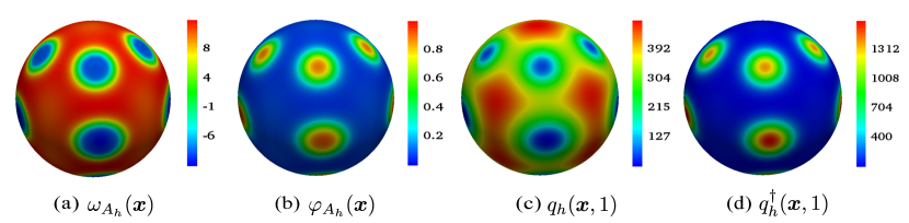
Figure 5: The equilibrium distributions of $\omega_{A_{h}}(\bm{x})$, $\varphi_{A_{h}}(\bm{x})$, $q_{h}(\bm{x},1)$ and $q_{h}^{\dagger}(\bm{x},1)$ on a spherical surface with a radius 3.56 $R_{g}$ when $\chi N=25,f=0.2$.

From these results, one can find that their spatial distributions are similar, however, $q_{h}(\bm{x},1)$ and $q_{h}^{\dagger}(\bm{x},1)$ vary more dramatically and have sharper interfaces. It can be expected that the error of numerical solutions decreases as the numerical errors of $q_{h}(\bm{x},1)$ and $q_{h}^{\dagger}(\bm{x},1)$ decrease. Therefore using $q_{h}(\bm{x},1)$ and $q_{h}^{\dagger}(\bm{x},1)$ as the indicator function to obtain the posterior error estimator $e_{\tau}$ is a proper choice. Concretely, $e_{\tau}$ can be chosen as

$$e_{\tau}=\frac{\|G_{h}q_{h}(\bm{x},1)\|_{\tau}+\|G_{h}q_{h}^{\dagger}(\bm{x},1)\|_{\tau}}{2}.$$ (19)

Besides the error estimator $e_{\tau}$, the mesh marking strategy is also crucial. Classic marking strategies, including the maximum criterion [30] and the $L^{2}$ criterion [31], usually refine or coarsen marked elements one time in each adaptive process. It may make less use of the information of the posterior error estimator. To improve it, we propose a new marking strategy, called the Log criterion, as follows

$$n_{\tau}=\left[\log_{2}\frac{e_{\tau}}{\theta\bar{e}}\right],$$ (20)

where $\theta$ is a positive constant, $\bar{e}$ is the mean value of estimators $e_{\tau}$ on all cells, and $[\cdot]$ is the nearest integer function. $n_{\tau}=0$, $n_{\tau}>0$ and $n_{\tau}<0$ represent that element $\tau$ is unchanged, refined $n_{\tau}$ times, and coarsened $|n_{\tau}|$ times, respectively. This new marking strategy does not only denote which mesh element $\tau$ needs to be changed, but also provides the times of refinement or coarseness. In our SCFT calculations, we choose a widely used “red-green-refinement” method to refine and coarsen the mesh element [32]. To better demonstrate the performance of the Log marking strategy, we take the Poisson equation in L-shape domain with Dirichlet boundary condition as an example and compare it with $L^{2}$ marking method in the Appendix section.

3.4 Surface integral

In this subsection, we discuss the integral method on an arbitrary curved surface. We use the symmetrical quadrature rules for triangle element [35]. Notice that, the quadrature points are given in the form of barycentric coordinates. Let $\{\bm{\lambda}_{j}\}_{j=0}^{\mathcal{J}-1}$ and $\{w_{j}\}_{j=0}^{\mathcal{J}-1}$ be the quadrature points and weights, respectively. For each $\bm{\lambda}_{j}$, one can easily obtain a unique point $\bm{x}_{j}\in\tau_{h}^{p}$ and a unique $\bm{u}_{j}\in\hat{\tau}$, respectively. We use the following integral formula to calculate the integral of finte element function $v_{h}$ defined on $\mathcal{M}_{h}^{p}$:

$$\int_{\mathcal{M}_{h}^{p}}v_{h}(\bm{x})\,\mathrm{d}\bm{x}=\sum_{\tau_{h}^{p}}\int_{\tau_{h}^{p}}v_{h}(\bm{x})\,\mathrm{d}\bm{x} =\sum_{\tau_{h}^{p}}\int_{\hat{\tau}}v_{h}(\bm{x}(\bm{u}))|\bm{J}(\bm{u})|\,\mathrm{d}\bm{u}$$

$$\approx|\hat{\tau}|\sum_{\tau_{h}^{p}}\sum_{j=0}^{\mathcal{J}-1}w_{j}v_{h}(\bm{x}_{j})|\bm{J}(\bm{u}_{j})|,$$

where $\bm{J}(\bm{u})$ is the Jacobi matrix of one-to-one mapping $\bm{x}:\hat{\tau}\mapsto\tau_{h}^{p}$ and $|\bm{J}(\bm{u})|$ is the corresponding determinant.

4 Contour discretization scheme and integration

4.1 Spectral deferred correction (SDC) method

In this subsection, we use the SDC method to discretize chain contour variable. The SDC scheme was originally proposed by Dutt et al. [36] to solve ordinary differential equations with an appropriate basic method, then used the residual equation to improve the approximation order of numerical solution. Unlike the classical deferred correction approach [36], the key idea of the SDC method is to use a spectral quadrature (see Sec 4.2) to integrate the contour derivative, which can achieve a high-accuracy numerical solution with a largely reduced number of quadrature points. In 2019, Ceniceros [37] firstly introduced the SDC method into the SCFT calculations. He chose the second-order implicit-explicit Runge-Kutta method as the basic solver to discretize the contour derivative, then used the SDC technique to improve the numerical precision. We follow a similar idea in this work but use a variable step size Crank-Nicholson method as the basic solver to compute propagator equations. The concrete implementation is given as follows.

The Crank-Nicholson method with variable time step size for semi-discrete propagator equation (16) is

$$\bm{M}\frac{\bm{q}^{n+1}-\bm{q}^{n}}{\delta t_{n}}=-\frac{1}{2}(\bm{A}+\bm{F})(\bm{q}^{n+1}+\bm{q}^{n}),\quad n=0,1,\dots,N_{t}-1,$$ (21)

where $\delta t_{n}=t_{n+1}-t_{n}$ is the time step size, $t_{n}$ ($n=0,1,2,\dots,N_{t}-1$) is the Chebyshev node [38]. Solving the above equation (21) can obtain the initial numerical solution $\bm{q}^{[0]}(t)$. Then we use the SDC scheme to achieve a high-accuracy numerical solution. We integrate the semi-discrete equation (16) along the contour variable $t$

$$\bm{M}\bm{q}(t)=\bm{M}\bm{q}(0)+\int_{0}^{t}\left[(-\bm{A}-\bm{F})\bm{q}(\tau)\right]d\tau.$$ (22)

The error between the numerical solution $\bm{q}^{[0]}(t)$ and the exact semi-discrete solution $\bm{q}(t)$ is

$$\bm{e}^{[0]}(t)=\bm{q}(t)-\bm{q}^{[0]}(t).$$ (23)

The error integration equation

$$\bm{M}\bm{e}^{[0]}(t)= \int_{0}^{t}\left[(-\bm{A}-\bm{F})\bm{e}^{[0]}(\tau)\right]d\tau+\bm{\gamma}^{[0]}(t),$$ (24)

can also be solved by the variable step size CN scheme (21) and the residual equation

$$\bm{\gamma}^{[0]}(t)=\bm{M}\bm{q}(0)+\int_{0}^{t}\left[\left(-\bm{A}-\bm{F}\right)\bm{q}^{[0]}(\tau)\right]d\tau-\bm{M}\bm{q}^{[0]}(t),$$ (25)

is computed by the Clenshaw-Curtis quadrature integral method as presented in Sec. 4.2. Then the corrected numerical solution is

$$\bm{q}^{[1]}(t)=\bm{q}^{[0]}(t)+\bm{\bm{e}}^{[0]}(t).$$ (26)

Repeating the above process, one can obtain $\bm{q}^{[2]},\dots,\bm{q}^{[J]}$, $J$ is the pre-determined number of deferred corrections. The convergent order of deferred correction solution along the contour variable is

$$\|\bm{q}(t)-\bm{q}^{[J]}(t)\|=O((\delta t)^{m(J+1)}),$$ (27)

where $\delta t=\max\{\delta t_{n}\}_{n=0}^{N_{t}-1}$, $m$ is the order of the basic numerical scheme to solve Eqns. (16) and (24). For the CN scheme, $m=2$.

4.2 Spectral integral method along the contour variable

In this subsection, we present the Clenshaw-Curtis quadrature method [37] to solve the residual equation (25) and evaluate the density functions (4) and (5), which has the spectral accuracy for smooth integrand function [39]. Concretely, assume $g(t)$, $t\in[a,b]$ is a smooth function, the Chebyshev-Gauss quadrature scheme is

$$\int_{a}^{b}g(t)\,dt =\frac{b-a}{2}\int_{-1}^{1}g(s)\,ds$$ (28)

$$\approx\left\{\begin{array}[]{ll}\dfrac{b-a}{2}\left[a_{0}+\sum\limits_{k=2\atop k\,\text{is\ even}}^{{N_{t}}-2}\left(\dfrac{2a_{k}}{1-k^{2}}\right)+\dfrac{a_{N_{t}}}{1-N_{t}^{2}}\right],&\quad N_{t}\ \text{is even},\\ \\ \dfrac{b-a}{2}\left[a_{0}+\sum\limits_{k=2\atop k\,\text{is\ even }}^{{N_{t}}-1}\left(\dfrac{2a_{k}}{1-k^{2}}\right)\right],&\quad N_{t}\ \text{is odd},\\ \end{array}\right.$$

where $a_{k}$, $k=0,1,\cdots,N_{t}$, is the discrete cosine transform coefficient of $g$.

5 Numerical results

In this section, we give several numerical examples to demonstrate the performance of the proposed methods. In the implementation, we use the linear ($p=1$), quadric ($p=2$), cubic ($p=3$) surface FEM, and adaptive surface FEM, to discretize the spatial variables, and the SDC method with a one-step correction to discretize the contour variable. The iteration step size $\lambda_{\pm}=2$ in the alternative direction explicit Euler method in the following computations. The following numerical example is implemented through FEALPy [40].

5.1 Efficiency

In this subsection, we use a parabolic equation with an exact solution and SCFT model on a spherical surface to examine the effectiveness of our numerical methods.

5.1.1 Efficiency of solving parabolic equation

As discussed above, the most computationally demanding part of the SCFT simulation is solving the PDEs for propagators which is a parabolic equation. We take a parabolic equation with an exact solution as an example to demonstrate the accuracy of our methods. Consider the parabolic equation defined on a unit sphere

$$\left\{\begin{array}[]{ll}{\dfrac{\partial}{\partial t}u(x,y,z,t)=\Delta_{\mathcal{M}}u(x,y,z,t)+f(x,y,z,t)},\\ \vspace{0.2cm}{u(x,y,z,0)=\sin(\pi x)\sin(\pi y)\sin(\pi z),}\end{array}\right.$$ (29)

where $(x,y,z)\in\{(x,y,z)~{}|~{}x^{2}+y^{2}+z^{2}=1\},~{}t\in[0,T]$, and

$$f(x,y,z,t) =\left(2\pi^{2}-1\right)e^{-t}\sin(\pi x)\sin(\pi y)\sin(\pi z)$$ (30)

$$+\frac{2\pi e^{-t}\left[z\sin(\pi x)\sin(\pi y)\cos(\pi z)+y\sin(\pi x)\sin(\pi z)\cos(\pi y)\right]}{x^{2}+y^{2}+z^{2}}$$

$$+\frac{2\pi e^{-t}\left[x\sin(\pi y)\sin(\pi z)\cos(\pi x)+xy\sin(\pi z)\cos(\pi x)\cos(\pi y)\right]}{x^{2}+y^{2}+z^{2}}$$

$$+\frac{2\pi^{2}e^{-t}\left[xz\sin(\pi y)\cos(\pi x)\cos(\pi z)+yz\sin(\pi x)\cos(\pi y)\cos(\pi z)\right]}{x^{2}+y^{2}+z^{2}},$$

with exact solution $u(x,y,z,t)=\sin(\pi x)\sin(\pi y)\sin(\pi z)e^{-t}$.

We analyze the spatial approximation order of surface FEMs and time approximation error obtained by CN and SDC schemes. Denote $\|\cdot\|_{\mathcal{M}}$ as the $L^{2}$ norm on a curved surface $\mathcal{M}$. Firstly, we observe the error of surface FEMs. We use the CN scheme with $\delta t=1\times 10^{-4}$ to ensure the contour discretization accuracy. As shown in Fig. 6 (a), the error order of linear, quadratic and cubic surface FEMs are $2$, $3$, and $4$, respectively, which is consistent with theoretical results.

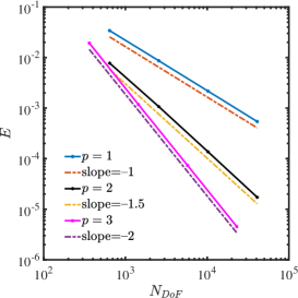
(a)

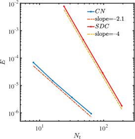
(b)

Figure 6: Comparison of logarithmic errors against the discretization nodes. (a) The spatial error of surface FEMs. $N_{DoF}$ is spatial DoFs. (b) The contour error order of CN and SDC schemes. $N_{t}$ is the number of contour points. $E=\|u_{I}(\cdot,T)-u_{h}(\cdot,T)\|_{\mathcal{M}^{p}_{h}}$, where $u_{I}(\cdot,T)$ is the value of exact solution $u(\cdot,T)$ interpolated from $\mathcal{M}$ to $\mathcal{M}^{p}_{h}$, $T=1$. The error order is the absolute value of the slope multiply by the dimension of variables, and the dimensions of space and time are $2$ and $1$, respectively.

Secondly, we present the error order of the contour discretization schemes, see Fig. 6 (b). We use the cubic surface FEM as the spatial discretization scheme to guarantee enough spatial discretization accuracy. When using the CN method, $5762$ initial spatial degrees of freedom (DoFs) are used. When applying the SDC scheme, the initial spatial DoFs are $362$. In these experiment, the spatial mesh grid will be refined once as the contour nodes are doubled. From Fig. 6 (b), one can find that the CN method has second-order precision. SDC method has $m(J+1)$-order precision, $m$ is the order of basic numerical method (CN), $J$ is the step of correction, here $m=2$, $J=1$. These results are also consistent with theoretical results.

Finally, we confirm the integral accuracy of the numerical solution along with the contour variable $t$. We use a modified fourth-order integral method, see (26) in [10], and the spectral integral scheme, as presented in the Sec. 4.2, to integrate $u^{CN}_{h}$ and $u^{SDC}_{h}$ from $0$ to $1$ for $t$ to obtain $U_{h}^{CN}$ and $U_{h}^{SDC}$, respectively. $u^{CN}_{h}$ and $u^{SDC}_{h}$ are the numerical solutions obtained by CN and SDC methods. The cubic surface FEM with $92162$ DoFs are used to ensure enough spatial precision. The integral value of the corresponding exact solution is discretized as $U^{e}_{h}$. The error is defined as

$$e^{W}=\|U^{e}_{h}-U^{W}_{h}\|_{\mathcal{M}_{h}^{p}},$$ (31)

where $W\in\{CN,SDC\}$. As Tab. 2 presents, the SDC method achieves the accuracy about $1.89\times 10^{-7}$ only requiring $16$ contour points, while the CN scheme needs $128$ nodes to reach the accuracy of $4.65\times 10^{-7}$. It is worth noting that the error value of SDC method is only reduced to about $2\times 10^{-7}$ due to the limitation of spatial discretization precision.

Table 2: The contour integral error of the 4-order integral scheme and the spectral integral method, $N_{t}$ is the number of contour points.

$N_{t}$	$e^{CN}$	$e^{SDC}$
8	5.08e-05	1.02e-06
16	1.32e-05	1.89e-07
32	3.52e-06	2.35e-07
64	1.08e-06	2.53e-07
128	4.65e-07	2.58e-07

5.1.2 Efficiency of SCFT calculations

We apply the high-order adaptive surface FEMs and contour discretization schemes to solve SCFT equations to demonstrate the power of our numerical methods. Due to the complicated SCFT self-consistent field system, we choose the value of the single chain partition function $Q$ as a metric to compare the accuracy of different numerical methods, since it is the integral value of the final result of the propagators. Here we use a sphere with a radius of $3.56R_{g}$ as the calculation surface, a high-order triangular mesh, see a schematic plot in Fig. 4 (b), to approximate the spherical surface. We obtain a spotted phase when parameters $\chi N=25$, $f=0.2$, as shown in Fig. 5 (b).

Firstly, we show the effectiveness of the contour discretization schemes. We use quadratic surface FEM with $163842$ DoFs to ensure enough spatial discretization accuracy. Certainly, one can choose linear and cubic FEMs, as long as the spatial discretization is accurate enough. In Fig. 7 (a), $Q_{ref}$ is numerically calculated by the SDC method with $560$ contour points. $E_{Q}=(Q-Q_{ref})/Q_{ref}$ is the relative error. Fig. 7 (a) shows that the SDC method converges much faster than the CN method.

Secondly, we investigate the accuracy of $p$-order ($p=1,2,3$) surface FEMs in the SCFT simulation. We use the SDC scheme with $200$ discretization points to guarantee enough accuracy in contour direction. In Fig. 7 (b), the reference value $Q_{ref}$ is numerically obtained by the cubic surface FEM with $92162$ DoFs. $E_{Q}=(Q-Q_{ref})/Q_{ref}$ is the relative error. One can observe that, compared with the linear surface FEM, the quadric and cubic surface FEMs have faster convergent rates.

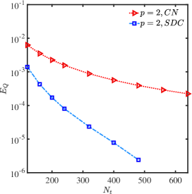
(a)

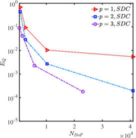
(b)

Figure 7: The convergence of single chain partition function $Q$ computed by different numerical schemes. $E_{Q}$ is the relative error. $N_{DoF}$ is spatial DoFs. (a) $Q$ obtained by the CN and SDC scheme as the contour point $N_{t}$ increases, and quadratic surface FEM with $163842$ DoFs is employed to discretize the spatial variables. (b) $Q$ computed by the linear, quadratic, and cubic surface FEMs with an increase of $N_{DoF}$, and the SDC scheme with $200$ points is applied to discretize the contour variable.

5.2 Adaptive surface FEM

In this subsection, we illustrate the performance of adaptive mesh method from two parts: the computational cost to achieve the same precise level and the application to strongly segregated systems compared with the uniform mesh approach. In this subsection, we choose quadratic surface FEM in the adaptive mesh method. Certainly, one can apply arbitrary order surface FEMs in this adaptive mesh approach. The SDC scheme with $200$ contour points is used to guarantee the contour discretization accuracy.

Firstly, we discuss the effectiveness of adaptive mesh method through an example in which the parameter $\chi N=25$, $f=0.2$, and a computational domain is a sphere with a radius of $3.56R_{g}$. The triangular uniform mesh with $10242$ DoFs is used as the initial mesh of the system. The adaptive process begins when the SCFT iteration reaches the maximum step $500$ or the reference estimator satisfies

$$e_{ref}=\sigma(e_{\tau})/(\max(e_{\tau})-\min(e_{\tau}))<0.1,$$

where $\sigma(e_{\tau})$ is the standard deviation of $e_{\tau}$, as defined in Eqn. (17). The stop condition of the adaptive process is the Hamiltonian discrepancy less than $1.0\times 10^{-6}$. The final convergent structure is the spotted phase, as shown in Fig. 5 (b). Fig. 8 (a) presents the final adaptive mesh with $61202$ DoFs. From these results, one can find that the adaptive approach can detect the sharp interface and damped internal structure to assign the mesh distribution reasonably. The change of Hamiltonian $H$ during the adaptive process is given in Fig. 8 (b).

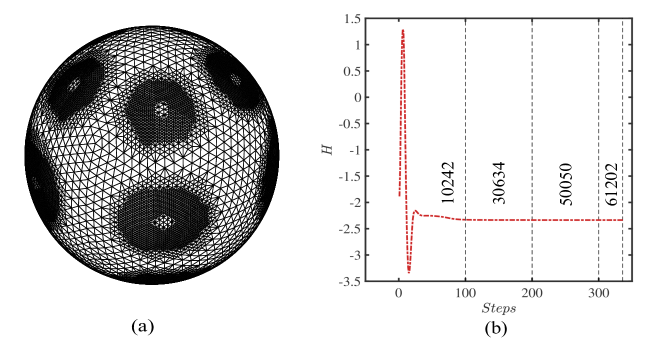
Figure 8: (a) The final adaptive mesh. (b) The change of Hamiltonian $H$ during the adaptive procedure. The numbers between two dotted lines represent spatial DoFs in the adaptive process.

Secondly, we further compare the values of $Q$ and $H$ when using the adaptive mesh and uniform mesh approaches. Fig. 9 shows the convergence of $Q$ and $H$ by the uniform mesh method. $E_{Q}=(Q-Q_{ref})/Q_{ref}$ and $E_{H}=(H-H_{ref})/H_{ref}$ are the relative errors. The reference values $Q_{ref}$ and $H_{ref}$ are obtained by the adaptive mesh method with $61202$ DoFs.

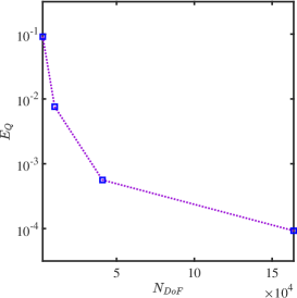
(a)

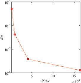
(b)

Figure 9: A comparison between the adaptive mesh method and the uniform mesh approach when $\chi N=25,f=0.2$. The relative error (a) $E_{Q}$ and (b) $E_{H}$.

Tab. 3 presents the finally converged values of $Q$ and $H$ through the adaptive mesh and uniform mesh methods. One can observe that $Q$ and $H$ obtained by the uniform mesh method converge to the adaptive mesh approach from these numerical results. The uniform mesh method needs $163842$ DoFs to achieve the same error level, which is $2.68$ times than the adaptive mesh approach does.

Table 3: The converged values of $Q$ and $H$ otained by the adaptive and uniform mesh methods when $\chi N=25,f=0.2$.

Method	$N_{DoF}$	$Q$	$H$
Adaptive	61202	3.2329e+02	-2.336168
Uniform	163842	3.2326e+02	-2.336165

Thirdly, we apply the adaptive mesh method to the strongly segregated systems on a spherical surface with a radius of $3.56R_{g}$. Tab. 4 gives numerical results of $\chi N$ from $25$ to $60$ and $f=0.2$. In Tab. 4, $N^{Adap}_{DoF}$ is the spatial DoFs of the adaptive mesh scheme. $h_{min}$ is the minimum size of the adaptive mesh. $N^{Uni}_{DoF}$ is the estimated DoFs of the uniform mesh method by making the mesh size equal $h_{min}$. In relatively strong segregation regime, its initial values come from the converged results of relatively weak segregated systems. For example, the initial values of $\chi N=30$ system come from the converged results of $\chi N=25$ system by the interpolation approach.

Table 4: Numerical results by the adaptive surface FEM for strongly segregated systems with different $\chi N$ and $f=0.2$. $N^{Adap}_{DoF}$ is spatial DoFs of the adaptive mesh method. $h_{min}$ is the minimum size of the adaptive mesh element. $N^{Uni}_{DoF}$ is the estimated spatial DoFs of the uniform mesh scheme with mesh size $h_{min}$.

$\chi N$	SCFT iterations	$h_{min}$	$N^{Adap}_{DoF}$	$N^{Uni}_{DoF}$	$N^{Adap}_{DoF}/N^{Uni}_{DoF}(\%)$
25	336	1.72e-02	61202	163842	37.3%
30	40	1.72e-02	68130	163842	41.5%
35	70	8.64e-03	79146	655362	12.1%
40	69	8.64e-03	113554	655362	17.3%
45	72	8.64e-03	153634	655362	23.4%
50	76	8.64e-03	178058	655362	27.1%
55	79	8.64e-03	198290	655362	30.2%
60	49	4.32e-03	219634	2621442	8.37%

Correspondingly, Fig. 10 shows the distribution of converged adaptive meshes and equilibrium structures for different $\chi N$. It is obvious that the interface narrows as $\chi N$ increases. From these results, one can find that spatial DoFs and iteration steps of the adaptive mesh method increase mildly as $\chi N$ increases. The adaptive mesh approach can significantly save the computational amount compared with the uniform mesh approach, even up to $91.63\%$ when $\chi N=60$, $f=0.2$. This is attributed to the adaptive mesh approach that can efficiently arrange two-scale mesh grids for the sharp interface and damped internal morphology by locally refining and coarsening mesh grids.

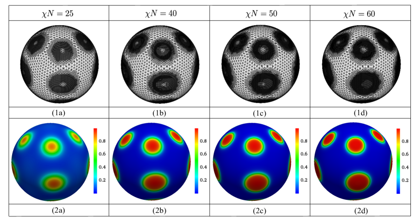
Figure 10: The adaptive meshes and equilibrium structures of $f=0.2$ and different interaction parameter $\chi N$.

5.3 Self-assembled structures on general curved surfaces

This subsection presents the application of the adaptive mesh approach on five curved surfaces for different $\chi N$ and $f$. Fig. 11 shows the converged results of adaptive meshes and morphologies on three closed surfaces, and Fig. 12 provides the corresponding results on two open surfaces. The homogeneous Neumann boundary condition is used for open surfaces. Tab. 5 presents the corresponding calculated data. From these results, one can find that the adaptive mesh method is efficient and saves spatial DoFs both on closed and open surfaces. For example, the adaptive mesh method can save the computational amount up to $89\%$ for computing the spotted phase on the parabolic surface when $\chi N=40$, $f=0.2$.

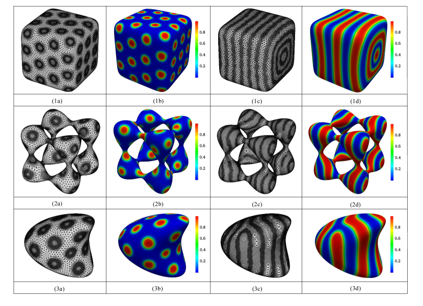
Figure 11: Applying the adaptive mesh method for solving SCFT on three closed curved surfaces (1). Squared surface; (2). Quartics surface; (3). Heart surface. The second and fourth columns present the spotted phase and strip phase, respectively. The first and third columns show the corresponding adaptive meshes. Model parameters are (1b) $[\chi N=45,f=0.2]$, (1d) $[\chi N=20,f=0.5]$, (2b) $[\chi N=35,f=0.2]$, (2d) $[\chi N=30,f=0.5]$, (3b) $[\chi N=45,f=0.2]$, (3d) $[\chi N=25,f=0.5]$. The calculated data are given in the Tab. 5.

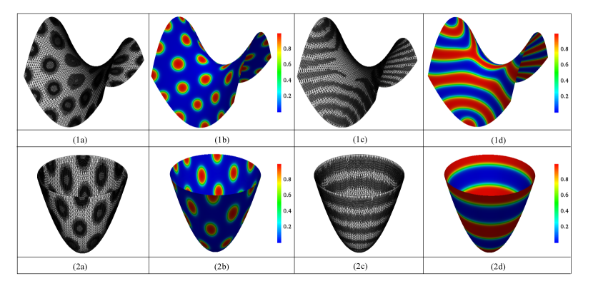
Figure 12: Applying the adaptive mesh method to solving SCFT on two open curved surfaces (1). Saddle surface and (2). Parabolic surface for relative strongly segregated systems. The second and fourth columns present the spotted phase and strip phase, respectively. The first and third columns show the corresponding adaptive meshes. Model parameters are (1b) $[\chi N=40,f=0.2]$, (1d) $[\chi N=20,f=0.5]$, (2b) $[\chi N=40,f=0.2]$, (2d) $[\chi N=35,f=0.5]$. The calculated data are shown in the Tab. 5.

Table 5: The computational data on five different curved surfaces as shown in Figs. 11 and 12. $N^{Adap}_{DoF}$ and $h_{min}$ are spatial DoFs and the minimum element size of the adaptive mesh approach, respectively. $N^{Uni}_{DoF}$ is the estimated spatial DoFs of the uniform mesh method with mesh size $h_{min}$.

Mesh	$h_{min}$	$N^{Adap}_{DoF}$	$N^{Uni}_{DoF}$	$N^{Adap}_{DoF}/N^{Uni}_{DoF}(\%)$
Fig. 11(1)(a)	7.756e-03	444114	1483060	30%
Fig. 11(1)(c)	2.458e-02	68414	93528	73%
Fig. 11(2)(a)	1.129e-02	103876	290272	35%
Fig. 11(2)(c)	1.039e-02	228576	356290	64%
Fig. 11(3)(a)	7.799e-03	131370	689928	19%
Fig. 11(3)(c)	1.505e-02	85238	172488	49%
Fig. 12(1)(a)	3.907e-03	179929	1052676	17%
Fig. 12(1)(c)	7.815e-03	47685	264196	18%
Fig. 12(2)(a)	3.272e-03	107919	1007300	11%
Fig. 12(2)(c)	3.272e-03	267297	1007300	26%

6 Conclusion

In this paper, we proposed an adaptive high-order surface FEM for solving SCFT equations on general curved surfaces. The high-order surface FEM was obtained through two aspects: high-order function space approximation and high-order geometrical surface approximation. To further reduce spatial DoFs, an efficient adaptive mesh method equipped with a new Log marking strategy was presented, which can make full use of the information of obtaining numerical results to refine or coarsen mesh. To improve the approximation order of the contour derivative, the SDC method was also used to address the contour variable. The resulting method can achieve high accuracy with fewer spatial and contour nodes and is suitable for solving strongly segregated systems. When computing strongly segregated systems, the superiority of the adaptive mesh method is even more pronounced, which can save spatial DoFs up to $91.63\%$ at most compared with the uniform mesh approach. In the future, we will apply these numerical methods to other polymer systems, for example, rigid chain systems.

Appendix: A comparison between Log and $L^{2}$ marking strategies

In this Appendix section, we take the Poisson equation (32) as an example to compare the Log with the traditional $L^{2}$ marking strategies.

$$-\Delta u=0, \text{ in }\Omega,$$ (32)

$$u=g, \text{ on }\partial\Omega,$$

where $\Omega=(-1,1)^{2}\backslash(0,1)\times(-1,0)$. Here we take the exact solution as $u_{e}=r^{2/3}\sin(2\theta/3)$, where $r,\theta$ are polar coordinates. Then the Dirichlet boundary condition $g$ can be determined by $u_{e}$.

We use the linear FEM to solve the equation and obtain a numerical solution $u_{h}$. Denote the error estimator on the element $\tau$ as

$$e_{\tau}=\|R_{h}u_{h}-\nabla u_{h}\|_{\tau},$$

where $R_{h}u_{h}$ is the simple average operator

$$R_{h}u_{h}(\bm{x}_{i}):=\frac{1}{n}\sum_{\bm{x}_{i}\in\tau,\tau\in\mathcal{K}}\nabla u_{h}(\bm{x}_{i})|_{\tau}.$$

$n$ is the number of element $\tau$ with $\bm{x}_{i}$ as a vertex, $\mathcal{K}$ denotes the set of elements in $\Omega$ with common vertex $\bm{x}_{i}$.

The Log marking strategy has been presented in Sec. 3.3. In this comparison, we set $\theta=1$ in (20) in the Log marking strategy. Before we go ahead, it is necessary to introduce the $L^{2}$ marking strategy. Let $\mathcal{A}$ be a set consisting of all elements which are required to be refined. The initial $\mathcal{A}$ is empty. In each adaptive iteration, $L^{2}$ marking strategy sorts element estimators $e_{\tau}$ in a descending order, and adds elements into $\mathcal{A}$ until

$$\sum_{\tau\in\mathcal{A}}e_{\tau}^{2}\geq\beta\sum_{\tau\in\Omega}e_{\tau}^{2},$$

where $\beta\in(0,1)$. In the following calculation we set $\beta=0.2$. We refine the mesh elements in $\mathcal{A}$ with “red-green-refinement” approach [32].

We perform the adaptive method to solve (32) through Log and $L^{2}$ marking strategies, respectively. Numerical results are shown in Tab. 6 and Fig. 13. We use $\|u_{e}-u_{h}\|_{0}$ with $L^{2}$-norm to measure the numerical error between exact solution $u_{e}$ and numerical solution $u_{h}$. When the numerical error reaches an level of about $2.4\times 10^{-6}$, two methods have almost same $N_{DoF}$. However, $L^{2}$ marking strategy requires $46$ adaptive iterations, while Log strategy only needs $10$ adaptive iterations. Correspondingly, the Log strategy saves $46.2\%$ CPU times. It is demonstrated that the Log strategy can save much CPU time in the adaptive method.

Table 6: The relative data for the $L^{2}$ and Log marking strategies at the error level $2.4\times 10^{-6}$.

Strategy	$N_{DoF}$	$\|u_{e}-u_{h}\|_{0}$	Iteration	CPU
$L^{2}$	135451	2.45e-06	46	108s
Log	138940	2.39e-06	10	58s

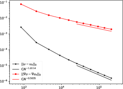
(a)

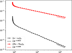
(b)

Figure 13: The comparison of errors with (a) Log and (b) $L^{2}$ marking strategies. The $x$-axis is $N_{DoF}$.

Fig. 14 shows the adaptive meshes obtained by two strategies when the error level is $1.0\times 10^{-4}$. As one can see, to achieve the same error level, the $Log$ marking strategy only needs $2$ iterations, while the second method needs $26$ iterations. At the same time, the refined meshes of the $Log$ marking strategy are concentrated near the singular points. In contrast, the refined meshes of the $L^{2}$ marking strategy spread to non-singular domain which does not need to be refined. These adaptive processes sufficiently demonstrate the efficiency of the new proposed Log marking strategy.

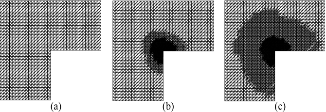
Figure 14: (a) Initial mesh. Adaptive meshes when the error level is $1.0\times 10^{-4}$: (b) the $2^{nd}$ iteration with Log marking strategy; (c) the $26^{th}$ iteration with $L^{2}$ marking strategy.

References

- [1] C.R. Stewart-Sloan, E.L. Thomas, Interplay of symmetries of block polymers and confining geometries, Eur. Polym. J. 47 (4) (2011) 630-646.
- [2] R.A. Segalman, Patterning with block copolymer thin films, Mater. Sci. Eng., R Rep. 46 (6) (2005) 191-226.
- [3] Y.Y. Wu, G.S. Cheng, K. Katsov, S.W. Sides, J.F. Wang, J. Tang, G.H. Fredrickson, M. Moskovits, G.D. Stucky, Composite mesostructures by nanoconfinement, Nat. Mater. 3 (11) (2004) 816-822.
- [4] H.Q. Xiang, K. Shin, T. Kim, S. Moon, T.J. McCarthy, T.P. Russell, The influence of confinement and curvature on the morphology of block copolymers, J. Polym. Sci. Part B 43 (2005) 3377-3383.
- [5] B. Yu, P.C. Sun, T.H. Chen, Q.H. Jin, D.T. Ding, B.H. Li, A.C. Shi, Confinement-induced novel morphologies of block copolymers, Phys. Rev. Lett. 96 (2006) 138306.
- [6] H. L. Deng, Y. C. Qiang, T. T. Zhang, W. Li, T. Yang. Chiral selection of single helix formed by diblock copolymers confined in nanopores. Nanoscale. 8 (2016) 15961-15969.
- [7] L.S. Zhang, L. Wang, J. Lin, Defect structures and ordering behaviours of diblock copolymers self-assembling on spherical substrates, Soft Matter 10 (35) (2014) 6713-6721.
- [8] J.F. Li, J. Fan, H.D. Zhang, F. Qiu, P. Tang, Y.L. Yang, Self-assembled pattern formation of block copolymers on the surface of the sphere using self- consistent field theory, Eur. Phys. J. E 20 (4) (2006) 449-457.
- [9] T.L. Chantawansri, A.W. Bosse, A. Hexemer, H.D. Ceniceros, C.J. Garciacervera, E.J. Kramer, G.H. Fredrickson, Self-consistent field theory simulations of block copolymer assembly on a sphere, Phys. Rev. E 75 (3) (2007) 031802.
- [10] H.Y. Wei, M. Xu, W. Si, K. Jiang, A finite element method of the self-consistent field theory on general curved surfaces, J. Comput. Phys. 387 (15) (2019) 230-244.
- [11] G.H. Fredrickson, The equilibrium theory of inhomogeneous polymers, Oxford University Press: New York (2006).
- [12] B. Vorselaars, J.U. Kim, T.L. Chantawansri, G.H. Fredrickson, M.W. Matsen, Self-consistent field theory for diblock copolymers grafted to a sphere, Soft Matter (7) (2011) 5128-5137.
- [13] J.F. Li, J. Fan, H.D. Zhang, F. Qiu, P. Tang, Y.L. Yang, Self-consistent field theory of block copolymers on a general curved surface, Eur. Phys. J. E 37 (3) (2014) 9973.
- [14] D.M. Ackerman, K. Delaney, G.H. Fredrickson, B. Ganapathysubramaniana, A finite element approach to self-consistent field theory calculations of multiblock polymers. J. Comput. Phys. 331 (2017) 280-296.
- [15] C.B. Macdonald, S.J. Ruuth, The implicit Closest Point Method for the numerical solution of partial differential equations on surfaces, SIAM J. Sci. Comput. 31 (6) (2009) 4330-4350.
- [16] S. Osher, R. Fedkiw, Level set methods: an overview and some recent results, J. Comput. Phys. 169 (2001) 463-502.
- [17] G. Dziuk, Finite elements for the Beltrami operator on arbitrary surfaces, in: Hildebrandt S., Leis R. (eds) Partial differential equations and calculus of variations. Lecture Notes in Mathematics, vol 1357. Springer, Berlin, Heidelbergv, (1988) 142-155.
- [18] A. Demlow, G. Dziuk, An adaptive finite element method for the Laplace-Beltrami operator on surfaces, SIAM J. Numer. Anal. 45 (2007) 421-442.
- [19] A. Demlow, Higher-order finite element methods and pointwise error estimates for elliptic problems on surfaces, SIAM J. Numer. Anal. 47 (2) (2009) 805-827.
- [20] B.Y. Li, Convergence of Dziuk’s semidiscrete finite element method for mean curvature flow of closed surfaces with high-order finite elements, SIAM J. Numer. Anal. 59 (2021), 1592–1617.
- [21] H.Y. Wei, L. Chen, Y.Q. Huang, Superconvergence and gradient recovery of linear finite elements for the Laplace-Beltrami operator on General surfaces, SIAM J. Numer. Anal. 48 (2010) 1920-1943.
- [22] A. Bonito, A. Demlow, A posteriori error estimates for the Laplace-Beltrami operator on parametric C2 surfaces, SIAM J. Numer. Anal. 57 (2019) 973-996.
- [23] G. Dziuk, C.M. Elliott, Finite element methods for surface PDEs, Acta Numerical 22 (2017) 289-396.
- [24] A. Bonito, A. Demlow, R.H. Nochetto, Finite element methods for the Laplace-Beltrami operator, Handbook of Numerical Analysis, 21 (2020) 1-103.
- [25] M.W. Matsen, The standard Gaussian model for block copolymer melts, J. Phys.: Condens. Matter 14 (2002) R21-R47.
- [26] K. Jiang, W.Q. Xu, P.W. Zhang, Analytic structure of the SCFT energy functional of multicomponent block copolymers, Commun. Comput. Phys. 17 (05) (2015) 1360-1387.
- [27] H.D. Ceniceros, G.H. Fredrickson. Numerical solution of polymer self-consistent field theory. Multiscale Model. Simul. 2 (03) (2004) 452-474.
- [28] H.T. Nguyen, p-adaptive and automatic hp-adaptive finite element methods for elliptic partial differential equations Ph.D. Thesis, Department of Mathematics, University of California, San Diego, La Jolla, CA (2010).
- [29] Y.Q. Huang, K. Jiang, N.Y. Yi, Some weighted averaging methods for gradient recovery, Adv. Appl. Math. Mech. 4 (02) (2012) 131-155.
- [30] H. Jarausch, On an adaptive grid refining technique for finite element approximations, SIAM J. Sci. and Stat. Comput. 7(04) (1986) 1105-1120.
- [31] W. Dörfler, A convergent adaptive algorithm for Poisson’s equation, SIAM J. Numer. Anal. 33(03) (1996) 1106-1124.
- [32] R.E. Bank, A.H. Sherman, A. Weiser, Refinement algorithms and data structures for regular local mesh refinement, Scientific computing (Montreal, Que., 1982), IMACS Trans. Sci. Comput., I, IMACS, New Brunswick, NJ, (1983) 3–17.
- [33] O.C. Zienkiewicz, R.L. Taylor, J.Z. Zhu, The finite element method: its basis and fundamentals[M]. Elsevier, (2013) 64-65.
- [34] D.A. Dunavant, High degree efficient symmetrical Gaussian quadrature rules for the triangle,Int J Numer Methods Eng, 21 (6) (1985) 1129-1148.
- [35] D. M. Williams, L. Shunn, A. Jameson, Symmetric quadrature rules for simplexes based on sphere close packed lattice arrangements[J], J. Comput. Appl. Math. 266 (2014) 18-38.
- [36] A. Dutt, L. Greengard, V. Rokhlin, Spectral deferred correction methods for ordinary differential equations, BIT Numer. Math. 40 (02) (2000) 241-266.
- [37] H.D. Ceniceros, Efficient order-adaptive methods for polymer self-consistent field theory, J. Comput. Phys. 386 (01) (2019) 9-21.
- [38] C.W. Clenshaw, A.R. Curtis, A method for numerical integration on an automatic computer, Numer. Math. 2 (01) (1960) 197-205.
- [39] L.N. Trefethen, Is Gauss quadrature better than Clenshaw-Curtis? SIAM Review 50 (01) (2008) 67-87.
- [40] H.Y. Wei and Y.Q. Huang, FEALPy: Finite element analysis library in Python, https://github.com/weihuayi/fealpy, Xiangtan University, 2017-2021.